Estimating Rice Agronomic Traits Using Drone-Collected Multispectral Imagery

Abstract

The knowledge of rice nitrogen (N) requirements and uptake capacity are fundamental for the development of improved N management. This paper presents empirical models for predicting agronomic traits that are relevant to yield and N requirements of rice (Oryza sativa L.) through remotely sensed data. Multiple linear regression models were constructed at key growth stages (at tillering and at booting), using as input reflectance values and vegetation indices obtained from a compact multispectral sensor (green, red, red-edge, and near-infrared channels) onboard an unmanned aerial vehicle (UAV). The models were constructed using field data and images from two consecutive years in a number of experimental rice plots in Greece (Thessaloniki Regional Unit), by applying four different N treatments (C0: 0 N kg∙ha⁻¹, C1: 80 N kg∙ha⁻¹, C2: 160 N kg∙ha⁻¹, and C4: 320 N kg∙ha⁻¹). Models for estimating the current crop status (e.g., N uptake at the time of image acquisition) and predicting the future one (e.g., N uptake of grains at maturity) were developed and evaluated. At the tillering stage, high accuracies (R² ≥ 0.8) were achieved for N uptake and biomass. At the booting stage, similarly high accuracies were achieved for yield, N concentration, N uptake, biomass, and plant height, using inputs from either two or three images. The results of the present study can be useful for providing N recommendations for the two top-dressing fertilizations in rice cultivation, through a cost-efficient workflow.

1. Introduction

Rice (Oryza sativa L.) is the second most cultivated cereal crop and the most consumed staple food in the world, since more than three billion people rely on rice as their primary source of food. Although it is predominant in Asia, rice has also been cultivated in Europe since the 15th century, mainly in Mediterranean countries including Italy, Spain, Portugal, Greece, and France (FAO database 2018). Rice is cultivated under a wide range of ecosystems, but more than 90% of the world’s rice production is harvested from irrigated or rainfed lowland rice fields [1]. Thus, increase in rice production is needed if the increased demand from population growth is to be met.

The use of nitrogen (N) fertilizer has changed the global N cycle markedly and has been causing various negative environmental consequences, such as eutrophication of surface water, global warming, and ozone layer depletion [2,3,4]. Modern production agriculture requires efficient, sustainable, and environmentally-sound management practices. N is a key factor in achieving optimum lowland rice grain yields [5]. It is the nutrient input normally required in large quantities for achieving high yields, but soils under these conditions are saturated, flooded, and anaerobic and, therefore, N use efficiency is low [6]. However, more than 50% of the applied N is not assimilated by the rice plant and it is lost through different mechanisms including ammonia volatilization, surface runoff, nitrification-denitrification, and leaching [7,8,9]. N₂O is the main greenhouse gas (GHG) related to agricultural soil emissions, essentially due to microbial transformation of nitrogen in the soil. This concerns N mineral fertilizers, manure spreading, and N from crop residues incorporated into the soil or lixiviation of surplus nitrogen. N₂O has high global warming potential (298 times higher than CO₂) and it should be minimized to reduce agricultural GHG emissions in total. The application of mineral N in the form of chemical fertilizers can also increase the N₂O emissions [10]. A recent study estimated the seasonal direct emission of N₂O from the paddy rice system in China (a country accounting for approximately 30% of the global rice production) to be 31.1 Gg N₂O-N for 2014, analyzing data from multiple studies [11]. Another recent study reported that intermittent flooding practices in rice can significantly increase N₂O emissions [12], although there is an active debate on this issue [13,14]. Therefore, N fertilizer management strategies that increase crop productivity and N use efficiency, while reducing negative environmental consequences, have to focus on parameters such as optimum time, rate, and spatial distribution methods that synchronize plant N requirements with N supply, in order to reduce N losses and maximize uptake of applied N in the crop [15]. Legislative measures adopted to comply with the Directive 91/676/EEC concerning the “Protection of Waters against Pollution caused by Nitrates from Agricultural Sources,” in some cases did not obtain the expected results and are not always accepted (or complied with) by farmers [16,17].

A key contributor to yield increases will be the efficient and effective use of nitrogen (N) fertilizer, which is relatively low in irrigated rice, because of rapid N losses from volatilization and denitrification in the soil-floodwater system [18]. The “4R” nutrient stewardship—applying the right nutrient source at the right rate, at the right time, and in the right place—is an innovative approach in fertilizer management [19]. Precision agriculture also has a positive impact on farm productivity and economics, as it provides higher or equal yields with lower production cost than conventional practices. The adoption of precision agriculture techniques for N management has the potential for improving agronomic, economic, and environmental efficiency in the use of such input [20].

Regarding the rest of the fertilization practices generally followed in Europe, phosphorous and potassium are supplied in the pre-planting stage at 50–70 kg∙ha⁻¹ and 100–150 kg∙ha⁻¹, respectively. The first fertilization intervention usually provides a nitrogen–phosphorous–potassium complex; it is carried out before the field flooding. The second supply is usually applied when rice plants are at the 3–5-leaf stage, at the beginning of tillering. A third fertilization can sometimes occur during panicle initiation. Sulfur can be applied using sulfuric fertilizers (NH₄ or K) and zinc is generally needed in soils with high pH, whereas calcium is needed in pathogenic soils with high salinity. The latter elements are used in Europe occasionally or after deficiencies [21].

A major challenge in N management through precision agriculture techniques is the accurate prediction and mapping of plant agronomic traits related to plant nutrient status and—most importantly—to N content. The traditional soil-based testing methods widely used for upland crops are not suitable for N recommendations in rice fields due to the flooding and complexity of N cycling in the rice paddy’s soil during the growing period [22]. Even before flooding, the available soil-N test is not accurate enough to lead to confident recommendations for N fertilizer applications [23]. Remote sensing technologies offer a viable alternative for deriving precise N recommendations in rice fields through the dynamic non-destructive estimation of plant N status throughout the growing season, along with predictions of other agronomic traits of interest (e.g., yield). Coupled with the rapidly advancing technology of unmanned aerial vehicle (UAV) platforms, they are nowadays starting to offer cost-effective solutions to various aspects of crop monitoring and sustainable crop management [24,25,26,27].

A few studies have proposed employing the traditional approach of active canopy sensors for estimating yield-related agronomic traits of rice plants, which can help in supporting precision N management [28,29,30,31,32,33,34,35]. For active field applications, these sensors could be installed on the machinery for real-time sensing, but such systems are not common in rice cultivation [36]. Most importantly, their use does become cost-inefficient (time and energy consuming) if the tractor must enter the rice paddy just for monitoring the N status, at growth stages other than the appropriate for fertilizer application or for weed and pest management. A substantial number of studies have also investigated the relationship between narrow-band vegetation indices (VIs) and various agronomic traits of rice plants [22,37,38,39,40,41,42,43,44,45,46,47,48,49,50,51,52,53,54]. The VIs are calculated from the spectral signatures obtained from handheld spectrometers, which are portable non-imaging hyperspectral sensors acquiring single spectral signatures from a small (typically circular) surface over the canopy. Most of these studies construct empirical models through linear regression for each possible pair of agronomic traits versus VIs, thus identifying the individual VIs that are highly correlated with each agronomic trait, but using the whole hyperspectral signatures as input to multivariable N status prediction models has also been proposed [45,48].

The results of the aforementioned studies are important, since they have identified the spectral wavelengths and/or VIs that are highly correlated with yield-related traits (e.g., [32,33,46,52]) or even proposed N recommendation methodologies based on remotely sensed data [28]. However, canopy-level spectral data from spectrometers becomes inappropriate for fine-scale precision farming, since that would require an extremely time-consuming and cost-inefficient dense sampling. In addition, the calculation of optimized VIs requires the sensor to incorporate bands at very specific wavelengths, which are typically not available in most multispectral sensors. It is true that compact hyperspectral sensors that can be mounted onboard UAVs (or movable structures above the canopy) have been developed the last few years and have been successfully employed for estimating rice agronomic traits [55,56,57]. Yet, the use of these systems is still limited in precision agriculture applications, their cost is relatively high, and processing such large volumes of data is quite challenging, although they have great potential for being operationally employed in the future.

Multispectral imaging sensors probably constitute the most appropriate system for precision agriculture applications in rice cultivation. Traditionally, satellite imagery has been employed for monitoring rice growth and agronomic traits. Medium-resolution satellite imagery (spatial resolution of 20–30 m) has been employed for providing rather coarse estimations of rice crop traits [58,59,60,61] or has been incorporated within rice growth simulation models [62]. High-resolution synthetic aperture radar (SAR) data have been employed for estimating morphological traits (most notably height) [63]. Recently, Sentinel-2 data have also been employed for estimating leaf area index (LAI) and plant N concentration of rice fields through empirical regression modeling, which were then used for producing N nutritional index maps [64]. Finally, a few studies have used commercial high-resolution (spatial resolution less than 10 m) satellite imagery to estimate N status [36,65,66] or within-field variability [61]. However, the most important drawback of high-resolution satellite images is their high cost for real-life applications, as almost all vendors enforce a large minimum area that can be ordered for a single image. If multiple images within the season are required for providing N recommendations and taking into consideration that rice paddies in a single cultivation have variable sowing dates—typically up to 30 days difference (due to genotypic differences in plant stages etc.)—the cost increases exponentially.

With the rapid development of UAV platforms (load capacity and flying autonomy), compact and lightweight multispectral sensors onboard UAVs seems to be the most direct and cost-efficient approach to precision agriculture in rice today. However, very few studies have been published that exploit such systems for estimating agronomic traits of rice plants. Initially, plain RGB cameras were used for estimating N status of rice plants [67,68], but these cameras are difficult to calibrate for different lighting conditions and they do not incorporate a near-infrared (NIR) channel that is required for the calculation of most VIs. Modifying the camera with a polarizing filter could solve the latter problem [69], but the sensor’s spectral response is still not appropriate for accurate calculation of most VIs, which require specific ranges of wavelengths. Good correlations of specific VIs calculated from multispectral sensors (RGB plus NIR channel) and measurements from chlorophyll meters (SPAD meter) have been reported [70,71]. However, estimating leaf N content from SPAD readings is not straightforward, since significant variability has been observed between SPAD values and both leaf chlorophyll [72,73,74] and leaf N [75,76,77] content. Finally, Lu et al. [78] has tested the potential of a 5-band multispectral sensor (RGB plus red-edge (RE) and NIR channels) onboard a UAV for estimating LAI and N content of rice plants, through simple linear regression. Medium to high correlations were reported at the panicle growing stage—close to the second top-dressing fertilization (TdF)—with lower coefficient of determination (R²) values reported for the stem elongation stage (close to the first TdF). However, their experimentation considered field data from a single growing season, and the lower R² values reported for the stem elongation stage suggest that multiple remote sensing variables must be considered simultaneously for increasing the modeling accuracy.

The objective of the current paper is to present empirical models for predicting agronomic traits of rice plants through remotely-sensed multispectral imagery. Models for predicting plant height, aboveground biomass, N concentration, Ν uptake, grain yield, and harvest index have been constructed following a multiple linear regression approach at different growth stages (at tillering and at booting), using as input reflectance values and VIs obtained from a compact four-band sensor (green, red, narrow-band RE, and NIR channels) onboard a UAV. The models were constructed using field data and images from two consecutive years in a number of experimental rice plots in Greece, employing different N treatments. Models for both estimating the current crop status (e.g., N uptake at the time of image acquisition) and predicting the future one (e.g., N uptake of grains at maturity) were developed and evaluated. To the best of our knowledge, this is the first study that presents such a comprehensive analysis for estimating various yield-related agronomic traits of rice plants during the growing season from UAV-collected multispectral data.

2. Materials and Methods

2.1. Field Experiments

Two field experiments were conducted in two consecutive years, 2016 and 2017, at the Experimental Station of Kalochori, Thessaloniki, Greece (40°36′58.75″N, 22°49′51.16″E in WGS 84 spatial reference system). The size of each experimental plot area was 11 m² (5 × 2.5 m) and arranged in a randomized complete block design with five replications for each treatment (Figure 1). The plots were fertilized with a novel bio-fertilizer (RBBf), developed at the Hellenic Agricultural Organization – DEMETER, in the framework of the H2020 project AGROCYCLE. The RBBf comprised 74% rice industrial co-products, chicken manure, zeolite, a compost accelerator by adding Aspergilus spp. (fungi), Bacillus spp. (bacteria), and larvae of the insects Hermetia illucens and Cetonia aurata. All raw materials were placed into a custom-made automatic compost bin of 1.5 tons capacity and left for at least 40 days to complete the composting process (i.e., when the C/N ratio reached a value lower than 20). The experiment consisted of four fertilization treatments: 1) 0 N kg∙ha⁻¹—untreated control (C0); 2) 80 N kg∙ha⁻¹ of RBBf (C1); 3) 160 N kg∙ha⁻¹ of RBBf—standard local practice for rice cultivation (C2); and 4) 320 N kg∙ha⁻¹ RBBf (C3). Seeds of the japonica type Greek commercial variety DION—belonging to the European Core Collection (http://tropgenedb.cirad.fr)—were directly seeded into the flooded plots on 2 June 2016 and 9 June 2017, respectively. The fertilization scheme followed the local and international standard practices for rice cultivation, where the amount is divided in three increments: 40% of the N–P–K are incorporated as basal before flooding, 40% is applied at the tillering stage, and similarly the rest (20%) at the panicle initiation stage. Besides fertilization, all the rest of the common practices were applied. The whole experiment was harvested when the plants reached the physiological maturity stage on October 6, 2016 and October 10, 2017, respectively.

Soil sampling was carried out prior to flooding, with three samples being collected as bulk from different field points according to standard soil field sampling methods. The soil analysis average results were sand = 30%, silk = 18%, loam = 52%, pH = 7.6, organic matter = 2%, N = 0.05%, P = 0.012%, K = 0.24%, Ca = 0.2%, and Zn = 0.012%. However, no significant variations within the different samples collected from the whole experimentation area were observed. Standard cultural practices for rice cultivation were conducted including harrowing, tillage, and lazier leveling. The plot embankments were made by hand, as were the RBBf application and sowing. Weed control was performed chemically in the whole period of herbicide application according to the local standard practices. The irrigation water is of a very good quality (0.7 dS) in the area, without any traces of agrochemical residuals since it is checked very frequently from the local irrigation organization. After harvesting, the whole plants were removed from the paddies, whereas the crop residuals—including 2–3 cm culm and the roots—remained in the soil and were incorporated for decomposition until the next year. In the second year of the experimentation, we chose not to alter the position of each paddy-treatment, to avoid mixing of the different treatments throughout the experimentation.

During the experimentation period, the following traits were assessed at the appropriate BBCH-scale stages [79,80]: (1) plant height (PH; cm), by measuring the main stem of 30 random rice plants per plot; (2) total biomass (BT; tn∙ha⁻¹), by cutting 0.25m² square plots of the whole aboveground plant biomass and weighing it after 48 h of air oven drying at 70 °C until constant weight; (3) N concentration (NC; %), determined by the macro-Kjeldahl procedure [81]; (4) N uptake (NU; kg∙ha⁻¹), estimated as total biomass × N concentration [36]; (5) grain yield (Yield; tn∙ha⁻¹); and (6) harvest index (HI), estimated as grain yield / (total dry matter + grain yield). Harvest index is the ratio of grain yield to total biomass and is considered as a measure of biological success in partitioning assimilated photosynthate to the harvestable product [82]. The traits that change during the season (PH, BT, NC, and NU) were measured at BBCH scale: stage 25 (before the first TdF), stage 45 (at booting, approximately 5 days before the second TdF), and stage 99 (harvesting). The timings of the first two measurements coincided with the first and last UAV image acquisitions (see next subsection). At harvesting, NC and NU of stem and leaves only (NCSL and NUSL, respectively) and of grain (NCG and NUG, respectively) were also assessed. Similarly, biomass of stem and leaves only (BSL) was considered as an additional independent trait. Conversely, PH at maturity was not considered, since the parameter does not change after the full heading stage (BBCH 59 to 60).

Table 1. Summary description of the rice agronomic traits considered in this study.

Abbreviation	Description	Units
PH25	Plant height at BBCH 25	cm
PH45	Plant height at BBCH 45	cm
BT25	Total aboveground biomass at BBCH 25	tn∙ha−1
BT45	Total aboveground biomass at BBCH 45	tn∙ha−1
BT99	Total aboveground biomass at maturity	tn∙ha−1
BSL99	Biomass of stem and leaves at maturity	tn∙ha−1
Yield	Yield	tn∙ha−1
HI	Harvest index	—
NC25	Plant N concentration at BBCH 25	%
NC45	Plant N concentration at BBCH 45	%
NC99	Plant N concentration at maturity	%
NCSL99	N concentration of stem and leaves at maturity	%
NCG	N concentration of grains at maturity	%
NU25	Plant N uptake at BBCH 25	kg∙ha−1
NU45	Plant N uptake at BBCH 45	kg∙ha−1
NU99	Plant N uptake at maturity	kg∙ha−1
NUSL99	N uptake of stem and leaves at maturity	kg∙ha−1
NUG	N uptake of grains at maturity	kg∙ha−1

summarizes all agronomic traits considered in this study, which are used as dependent variables of the predictive models.

2.2. UAV Imagery and Preprocessing

We used the Parrot^® Sequoia™ multispectral imaging sensor (Parrot Drones S.A.S, Paris, France), which captures the reflected light at four spectral bands with a field of view of 70.6°: green (G; 550 nm; 40 nm bandwidth), red (R; 660 nm; 40 nm bandwidth), red-edge (RE; 735 nm; 10 nm bandwidth), and near-infrared (NIR; 790 nm; 40 nm bandwidth). The camera was mounted on a DJI Phantom 4 quadcopter (DJI, Shenzhen, China) and it was also equipped with an irradiance sensor for measuring incident light, in order to correct for variable lighting conditions during the flight. Prior to each flight, ground images from a calibration target (AIRINOV Aircalib; AIRINOV, Paris, France) were acquired, in order to derive accurate reflectance values. The latter was a polyvinyl chloride (PVC) board with a gray target area silkscreen printing and ArUco tags for the albedo measurements of each band, which have been measured specifically for the Sequoia sensor. The flight plan was created automatically through the Atlas Flight application (MicaSense, Inc., Seattle, USA), choosing 80% overlap for both front-lap and side-lap, in order to assure an accurate orthomosaic creation. The single images were subsequently combined to create an orthophotomosaic using Pix4Dmapper Pro (Pix4D S.A., Lausanne, Switzerland), which employs an advanced structure from motion (SfM) workflow to derive accurate orthophotomosaics in absolute reflectance values. The derivation of absolute reflectance values is achieved by Pix4D taking into consideration both the calibration target images and the readings from the irradiance sensor in an automated workflow, without the need for the user to calibrate or otherwise process the original images. An overview of the typical acquisition procedures and required processing of UAV imagery can be found in [83].

During each growing season, three images were acquired over the study area (

Table 2. Dates, equivalent days after sowing (DAS), and BBCH stage code for the major treatments, field data collection, and unmanned aerial vehicle (UAV) image acquisitions performed in the experimental plots during the two years.

Treatment or Data Acquisition	Date	DAS	BBCH
	2016
Basal fertilization	2 June 2016	0	—
Sowing	2 June 2016	0	—
1st image acquisition and field data collection	5 July 2016	33	25
1st TdF	8 July 2016	36	26
2nd image acquisition and field data collection	15 July 2016	43	31
3rd image acquisition and field data collection	17 August 2016	76	45
2nd TdF	22 August 2016	81	49
Harvesting	6 October 2016	126	99
	2017
Basal fertilization	8 June 2017	−1	—
Sowing	9 June 2017	0	—
1st image acquisition and field data collection	16 July 2017	37	25
1st TdF	18 July 2017	39	26
2nd image acquisition and field data collection	25 July 2017	46	31
3rd image acquisition and field data collection	18 August 2017	70	45
2nd TdF	23 August 2017	75	49
Harvesting	10 October 2017	123	99

). The drone was flown at a height of 30 m above ground level, resulting in an orthophotomosaic with spatial resolution of approximately 2.5 cm. A total of 35 VIs were calculated from each image (

Table 3. Summary of vegetation indices considered in this study. Camera channels are reported as G: green, R: red, RE: red-edge, and NIR: near-infrared.

Acronym	Name	Formula	Introduced in
DVI	Difference Vegetation Index (VI)	$\mathrm{NIR}-\mathrm{R}$	[84]
NDVI	Normalized difference VI	$\left(\mathrm{NIR}-\mathrm{R}\right)/\left(\mathrm{NIR}+\mathrm{R}\right)$	[85]
RVI	Ratio VI (also simple ratio (SR))	$\mathrm{NIR}/\mathrm{R}$	[86]
mSR	Modified simple ratio	$\left(\mathrm{NIR}/\mathrm{R}-1\right)/\sqrt{\left(\mathrm{NIR}/\mathrm{R}+1\right)}$	[87]
TNDVI	Transformed NDVI	$\sqrt{\left(\mathrm{NIR}-\mathrm{R}\right)/\left(\mathrm{NIR}+\mathrm{R}\right)+0.5}$	[84]
RDVI	Renormalized DVI	$\left(\mathrm{NIR}-\mathrm{R}\right)/\sqrt{\left(\mathrm{NIR}+\mathrm{R}\right)}$	[88]
SAVI	Soil-adjusted VI	$1.5\cdot \left(\mathrm{NIR}-\mathrm{R}\right)/\left(\mathrm{NIR}+\mathrm{R}+0.5\right)$	[89]
OSAVI	Optimized SAVI	$1.16\cdot \left(\mathrm{NIR}-\mathrm{R}\right)/\left(\mathrm{NIR}+\mathrm{R}+0.16\right)$	[90]
MSAVI2	Modified SAVI 2	$0.5\cdot \left[2\mathrm{NIR}+1 - {\left(2\mathrm{NIR}+1\right)}^2-8\sqrt{\mathrm{NIR}-\mathrm{R}}\right]$	[91]
gDVI	Green DVI	$\mathrm{NIR}-\mathrm{G}$	[84]
gNDVI	Green NDVI	$\left(\mathrm{NIR}-\mathrm{G}\right)/\left(\mathrm{NIR}+\mathrm{G}\right)$	[92]
gRDVI	Green RDVI	$\left(\mathrm{NIR}-\mathrm{G}\right)/\sqrt{\left(\mathrm{NIR}+\mathrm{G}\right)}$	[32]
mSRG	Modified green simple ratio	$\left(\mathrm{NIR}/\mathrm{G}-1\right)/\sqrt{\left(\mathrm{NIR}/\mathrm{G}+1\right)}$	[32]
GSAVI	Green SAVI	$1.5\cdot \left(\mathrm{NIR}-\mathrm{G}\right)/\left(\mathrm{NIR}+\mathrm{G}+0.5\right)$	[93]
MGSAVI	Modified GSAVI	$0.5\cdot \left[2\mathrm{NIR}+1-\sqrt{{\left(2\mathrm{NIR}+1\right)}^2-8\left(\mathrm{NIR}-\mathrm{G}\right)}\right]$	[32]
NGI	Normalized green index	$\mathrm{G}/\left(\mathrm{NIR}+\mathrm{RE}+\mathrm{G}\right)$	[93]
GWDRVI	Green wide dynamic range VI	$\left(0.12\cdot \mathrm{NIR}-\mathrm{G}\right)/\left(0.12\cdot \mathrm{NIR}+\mathrm{G}\right)$	[32]
CIG	Green chlorophyll index	$\mathrm{NIR}/\mathrm{G}-1$	[94]
CIRE	Red-edge chlorophyll index	$\mathrm{NIR}/\mathrm{RE}-1$	[94]
TCARI	Transformed chlorophyll absorption ratio index	$3\cdot \left[\left(\mathrm{RE}-\mathrm{R}\right)-0.2\left(\mathrm{RE}-\mathrm{G}\right)\left(\mathrm{RE}/\mathrm{R}\right)\right]$	[95]
MCARI1	Modified chlorophyll absorption in reflectance index 1	$1.2\cdot \left[2.5\left(\mathrm{NIR}-\mathrm{R}\right)-1.3\left(\mathrm{NIR}-\mathrm{G}\right)\right]$	[96]
MCARI2	Modified chlorophyll absorption in reflectance index 2	$1.5\cdot \left[2.5\left(\mathrm{NIR}-\mathrm{R}\right)-1.3\left(\mathrm{NIR}-\mathrm{G}\right)\right] / \sqrt{{\left(2NIR+1\right)}^2-\left[6NIR-5\sqrt{R}\right]-0.5}$	[96]
TCARI/ OSAVI	TCARI to OSAVI	$\mathrm{TCARI}/\mathrm{OSAVI}$	[95]
REDVI	Red-edge DVI	$\mathrm{NIR}-\mathrm{RE}$	[32]
NDRE	Normalized difference red-edge index	$\left(\mathrm{NIR}-\mathrm{RE}\right)/\left(\mathrm{NIR}+\mathrm{RE}\right)$	[97]
RERDVI	Red-edge RDVI	$\left(\mathrm{NIR}-\mathrm{RE}\right)/\sqrt{\left(\mathrm{NIR}+\mathrm{RE}\right)}$	[32]
NNIR	Normalized NIR index	$\mathrm{NIR}/\left(\mathrm{NIR}+\mathrm{RE}+\mathrm{G}\right)$	[93]
REGNDVI	Red-edge GNDVI	$\left(\mathrm{RE}-\mathrm{G}\right)/\left(\mathrm{RE}+\mathrm{G}\right)$	[32]
REWDRVI	Red-edge wide dynamic range VI	$\left(0.12\cdot \mathrm{NIR}-\mathrm{RE}\right)/\left(0.12\cdot \mathrm{NIR}+\mathrm{RE}\right)$	[32]
MSRRE	Modified red-edge simple ratio	$\left(\mathrm{NIR}/\mathrm{RE}-1\right)/\sqrt{\left(\mathrm{NIR}/\mathrm{RE}+1\right)}$	[32]
MEVI	Modified enhanced VI	$2.5\cdot \left(\mathrm{NIR}-\mathrm{RE}\right)/\left(\mathrm{NIR}+6\mathrm{RE}-7.5\mathrm{G}+1\right)$	[32]
RESAVI	Red-edge SAVI	$1.5\cdot \left(\mathrm{NIR}-\mathrm{RE}\right)/\left(\mathrm{NIR}+\mathrm{RE}+0.5\right)$	[32]
MRESAVI	Modified RESAVI	$0.5\cdot \left[2\mathrm{NIR}+1-\sqrt{{\left(2\mathrm{NIR}+1\right)}^2-8\left(\mathrm{NIR}-\mathrm{RE}\right)}\right]$	[32]
MTCARI	Modified TCARI	$3\cdot \left[\left(\mathrm{NIR}-\mathrm{RE}\right)-0.2\left(\mathrm{NIR}-\mathrm{G}\right)\left(\mathrm{NIR}/\mathrm{RE}\right)\right]$	[32]
MRETVI	Modified RETVI	$1.2\cdot \left[1.2\left(\mathrm{NIR}-\mathrm{G}\right)-2.5\left(\mathrm{RE}-\mathrm{G}\right)\right]$	[32]

), which have been considered in rice-related studies for the estimation of agronomic traits. Subsequently, the area within each experimental plot was manually delineated (approximately 10 m²), taking care not to include the plots’ boundaries (the paddy’s embankments). For each plot, the average value of all pixels within the delineated area was calculated for each camera band and VI, which were subsequently used for the analysis. The final dataset comprised 40 samples, since the experiment comprised 20 plots (five replications for each of the four N treatments) and measurements were acquired for the two years of experimentation (2016 and 2017).

2.3. Regression Models

The union of the camera’s four bands and the 35 VIs were used as inputs for building the empirical models. The samples used for the analysis were the average value of the VIs and the camera’s bands—as mentioned in the previous section—together with the corresponding field data values (one of the traits for each model) for each plot and for the two years of experimentation. In order to maintain the models’ interpretability, we chose to create them through the simple least-square multiple linear regression [98] approach. All VIs were considered as potential inputs for the models, since N treatments affect, simultaneously, biomass, leaf area index, and chlorophyll content of all plants and, as such, any VI could possibly increase the accuracy of a model built for each trait. In other words, we cannot a priori assume that some VI is irrelevant with an agronomic trait. However, since the number of possible inputs was high (39 for the models built for the tillering stage and 78 or 117 for those built for the booting stage, as will be explained in the following), a subset of predictors had to be selected, in order to maintain the models’ interpretability and increase their generalization capabilities. Input selection was performed through the lasso (least absolute shrinkage and selection operator) [99], which is a regularization technique for performing linear regression. Lasso solves the minimization problem:

$$\underset{{\beta }_0, \beta }{\min }\left(\frac{1}{2N}{\displaystyle \sum }_{i=1}^N{\left(y_i-{\beta }_0+{\mathit{x}}_i^{\mathrm{T}}\cdot \mathit{\beta }\right)}^2+\lambda {\displaystyle \sum }_{j=1}^P\left|{\beta }_j\right|\right),$$

(1)

where $N$ is the number of data samples, $P$ is the number of predictors (input variables), ${\mathit{x}}_i$ is the input vector ($P$-dimensional column vector) for the $i$th data sample, $y_i$ is the corresponding output value, $\mathit{\beta }$ is the $P$-dimensional column vector of linear coefficients, ${\beta }_0$ is the intercept term, and $\lambda$ is the positive regularization parameter. Lasso incorporates the $L^1$ norm of $\mathit{\beta }$ into the minimization task, which forces a number of coefficients to become zero, thus identifying the redundant predictors. Prior to the analysis, the input data were standardized to zero mean and variance of one. The regularization parameter $\lambda$ was determined through a five-fold cross-validation procedure, considering a geometric sequence of 100 values, with the largest value being the one that produces a null model. The largest $\lambda$ value such that the mean squared error (MSE) was within one standard error of the minimum MSE was ultimately selected. The predictors with non-zero coefficients were maintained and a multiple linear regression model was constructed considering those predictors only. To increase the model’s interpretation, only linear terms were considered, without interactions. The whole analysis was performed within the statistical software MATLAB^® (MathWorks Inc., MA, USA).

For each agronomic trait, regression models at two crop stages were created using the field data from both years, following the image acquisition scheme presented in Table 2. The first category of models was built for the crop stage with BBCH 25, which corresponds to two to three days before the first TdF (at the tillering stage). The second category was built for the crop stage with BBCH 45, which corresponds to approximately five days before the second TdF (at the booting stage). For the former category of models, the models were built considering the input variables from only the first image, captured at stage with BBCH 25. For the latter category of models, two approaches were tested. The first one used the union of input variables from two images, those captured at BBCH 25 and BBCH 45. The second also considers the input variables from the intermediate image acquisition at BBCH 31, which corresponds approximately 7–10 days after the first TdF (see the DAS values in Table 2). The rationale for the latter was to include an intermediate input after the fertilization, in order to indirectly capture the effectiveness of the treatment, which could potentially increase the model’s predictive capabilities.

For each of the agronomic traits that changes during the season (plant height, N concentration, N uptake, and total biomass), one model was constructed for each stage considered, that is, for BBCH 25, 45, and 99 (harvested product, apart from plant height that does not change after booting). Obviously, for the models constructed before the second fertilization (BBCH 45, considering two or three images), predicting agronomic traits in previous stages (i.e., BBCH 25) has no practical use, since we actually try to predict a past state from the current status (which is not always possible). Hence, no models predicting agronomic traits at BBCH 25 were constructed at the booting stage. The models’ accuracy was assessed by means of the regression’s adjusted coefficient of determination (Adj. $R^2$), as well as the root mean square error (RMSE). Since RMSE’s magnitude depends on the magnitude of the data, we also report a relative measure of the modeling errors’ dispersion, namely, the coefficient of variation of the RMSE (CV_RMSE), expressed as a percentage:

$${\mathrm{CV}}_{\mathrm{RMSE}}=100\cdot \frac{\mathrm{RMSE}}{\overline{y}} (\%),$$

(2)

where $\overline{y}$ is the mean of the observed output values, that is, the mean of the field measurements for the agronomic trait the model is built for.

The Sequoia sensor incorporates a RE channel, which is an advantage for agronomic remote sensing studies, since it is sensitive to smaller changes of leaf health and plant stress in general. However, many other sensors do not have such a channel, but rather follow the channel configuration of many high-resolution satellite sensors (blue, green, red, and NIR). Since it would be interesting to apply our methodology with such sensors as well, we also conducted a second experiment where the whole process (lasso input selection and linear model building) was repeated without the VIs relying on RE. In this case, the number of possible inputs was 23, namely, Sequoia’s green, red, and NIR channels and the following VIs: DVI, NDVI, SR, mSR, TNDVI, RDVI, SAVI, OSAVI, MSAVI2, gDVI, gNDVI, gRDVI, mSR_G, GSAVI, MGSAVI, GWDRVI, CI_G, MCARI1, MCARI2, and MTCARI (see Table 3).

3. Results

During both rice cultivation periods, temperature and relative humidity were constantly recorded in order to compare the meteorological data sets.

Table 4. Monthly temperature and relative humidity during the growing seasons of the two years that the experiments were conducted. Minimum, maximum, and average values of each year are reported, averaged over each month.

Year	Month	Temperature (°C)			Relative Humidity (%)
		Minimum	Maximum	Average	Minimum	Maximum	Average
2016	June	20	32	26	38	95	74
	July	20	33	26	48	97	78
	August	18	34	25	52	99	85
	September	16	29	21	51	98	83
	October	13	25	18	48	80	66
2017	June	18	32	25	50	84	61
	July	19	34	26	53	96	73
	August	18	34	24	60	98	79
	September	14	32	21	52	97	78
	October	13	28	19	43	89	69

reports monthly averages of temperature and relative humidity during the two growing seasons of the experimentation. The second year (2017) was slightly colder and less humid; however, these differences were minor and it can be concluded that they could not induce alterations in the morphophysiology of the rice plants between the two experiments over the two years.

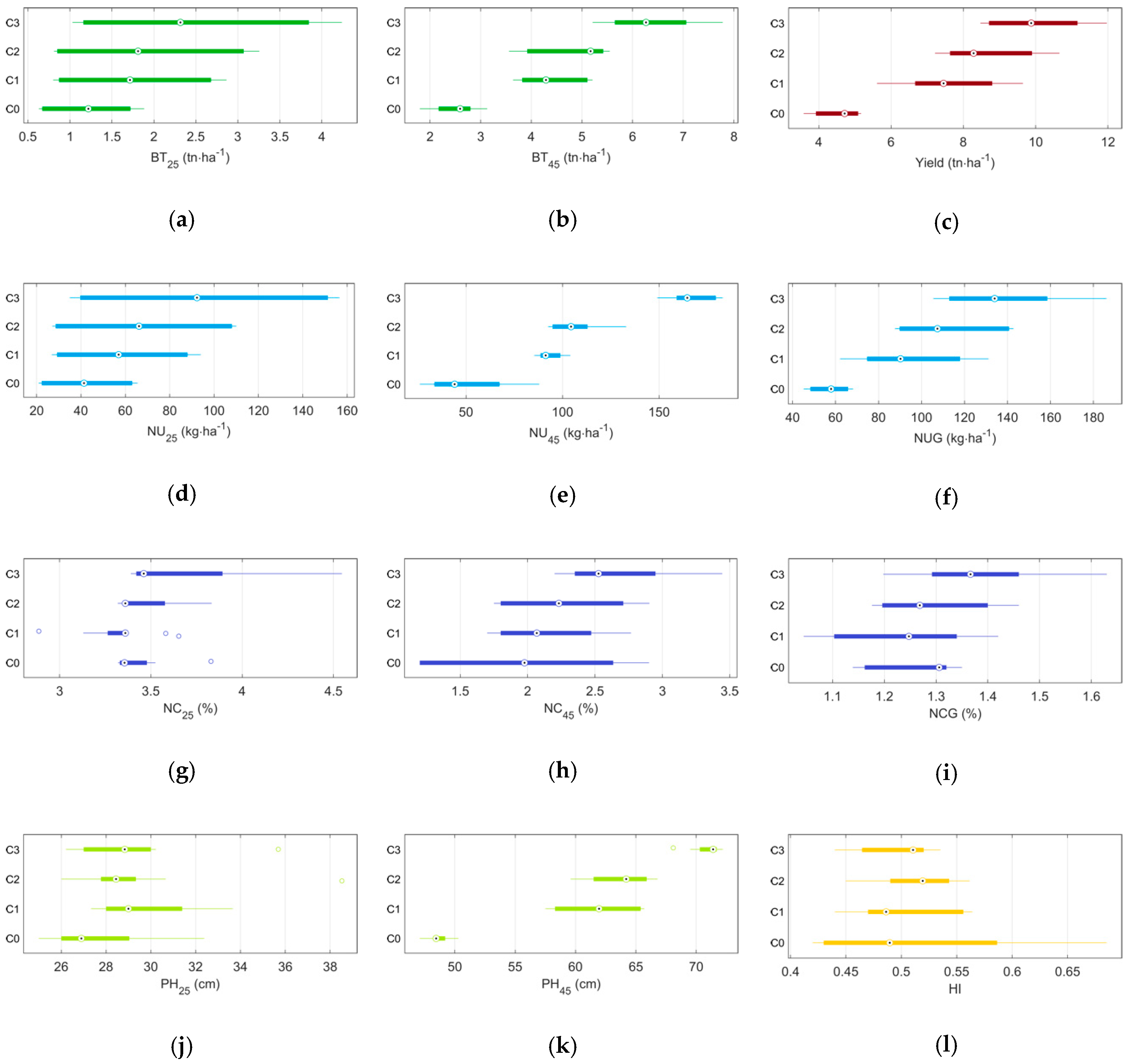
Figure 2 presents the differences of selected agronomic traits with respect to the fertilization treatment. Biomass, N uptake, and yield exhibit a rather expected trend, that is, higher values with increased amount of N fertilizer applied. Yield also exhibits the expected saturation with N fertilization, that is, the great differences in NU and BT between C2 (standard local practice) and C3 (double amount) at BBCH 45 were not fully reflected in yield differences. The variability was much higher at BBCH 25 (at tillering), since the canopy was not yet fully closed, due to the fact that the tillers were not completely developed and no TdF had been applied yet. As the growing season continued, the differences became more pronounced. The aforementioned trend was not clearly exhibited for N concentration and HI, which was also reflected in the modeling process that resulted in generally low predictive accuracy for those traits, as will be shown in the following. A possible explanation for this behavior is provided in the Discussion section. For completeness,

Table 5. Results of the one-way ANOVA test and Tukey’s honest significant difference (HSD) post-hoc test for the field-measured trait values against the different N treatments. The latter is presented by means of labeled groups, with two treatments that include the same letter denoting statistically non-significant differences between the mean values of the corresponding agronomic trait.

Trait	p-Value for ANOVA F-test	Tukey’s HSD Group
		C0	C1	C2	C3
PH25	0.3664	a	a	a	a
PH45	1.62∙10−20	c	b	b	a
BT25	0.0918	a	a	a	a
BT45	2.69∙10−13	c	b	b	a
BT99	3.59∙10−13	c	b	b	a
BSL99	8.25∙10−6	b	a	a	a
Yield	4.76∙10−11	c	b	ab	a
HI	0.8591	a	a	a	a
NC25	0.0342	ab	b	ab	a
NC45	0.0418	b	ab	ab	a
NC99	0.1044	a	a	a	a
NCSL99	0.0451	a	a	a	a
NCG	0.0315	ab	b	ab	a
NU25	0.0498	b	ab	ab	a
NU45	1.31∙10−18	c	b	b	a
NU99	0.0002	b	ab	a	a
NUSL99	0.0067	b	ab	a	a
NUG	6.3∙10−8	c	b	ab	a

reports the results of a one-way ANOVA statistical analysis, followed by Tukey’s honest significant difference (HSD) post-hoc test [100]. The results of the latter are compactly presented by means of labeled groups (letters), with two treatments that include the same letter denoting statistically non-significant differences between the mean values of the corresponding agronomic trait (e.g., treatments C1 and C2 for the Yield trait were not found to exhibit statistically significant differences, whereas treatments C0 and C1 for the same trait did).

Table 6. Summary statistics of the derived linear models, built considering all 39 possible inputs (before input selection). Adjusted coefficient of determination (R²), root mean square error (RMSE), coefficient of variation of the RMSE (CV_RMSE) (%), and number of predictors (#P) participating in each model are reported.

Trait	Models at Tillering (1 image)				Models at Booting (2 images)				Models at Booting (3 images)
	Adj. R2	RMSE	CVRMSE (%)	#P	Adj. R2	RMSE	CVRMSE (%)	#P	Adj. R2	RMSE	CVRMSE (%)	#P
PH25	0.12*	2.59	8.95	1	—	—	—	—	—	—	—	—
PH45	0.50	5.97	9.74	2	0.84	3.43	5.59	3	0.84	3.41	5.57	2
BT25	0.86	0.43	23.09	7	—	—	—	—	—	—	—	—
BT45	0.56	1.03	22.51	3	0.87	0.55	12.01	2	0.87	0.55	12.01	2
BT99	0.39	3.17	23.12	1	0.74	2.07	15.07	3	0.74	2.07	15.07	3
BSL99	0.54	1.99	25.89	3	0.72	1.54	20.07	3	0.72	1.55	20.23	4
Yield	0.61	1.47	19.12	4	0.77	1.13	14.73	5	0.80	1.06	13.73	6
HI	0.24	0.05	9.21	1	0.31	0.04	8.75	1	0.31	0.04	8.75	1
NC25	0.16	0.26	7.44	1	—	—	—	—	—	—	—	—
NC45	0.68	0.32	14.23	3	0.88	0.20	8.87	6	0.88	0.20	8.67	7
NC99	0.77	0.22	17.67	5	0.70	0.25	19.98	3	0.85	0.18	14.29	6
NCSL99	0.70	0.28	30.97	5	0.86	0.20	21.49	11	0.80	0.23	25.43	6
NCG	0.57	0.08	6.49	3	0.64	0.08	5.95	3	0.72	0.07	5.24	4
NU25	0.80	19.70	29.84	3	—	—	—	—	—	—	—	—
NU45	0.50	31.88	30.51	3	0.86	16.72	16.00	3	0.86	16.72	16.00	3
NU99	0.68	60.63	33.10	4	0.69	59.24	32.34	3	0.75	53.94	29.45	4
NUSL99	0.68	40.20	48.97	5	0.93	18.48	22.51	12	0.82	29.85	36.37	7
NUG	0.58	24.79	24.53	5	0.75	19.02	18.81	5	0.83	15.89	15.72	8

* Statistically significant at a level of 0.05; all other models are statistically significant at a level of 0.01.

reports the accuracy measures (adjusted R², RMSE, and CV_RMSE) of all linear models constructed considering all 39 possible inputs (before input selection), along with the number of predictors (input variables) selected by means of the lasso approach. At the tillering stage (BBCH 25), high correlations were only observed for BT₂₅ and NU₂₅. Thus, this time point appeared to be too soon for predicting the future development of the plants, particularly, when the first TdF had not been applied yet. Nevertheless, BT₂₅ and NU₂₅ were considered the two most important traits to support N fertilization dose (units/ha) at tillering. The linear models constructed for the booting stage using two UAV images (at BBCH 25 and 45) exhibited high correlations for most of the agronomic traits. The models for biomass (BT₉₉ and BSL₉₉) and N concentration (NC₉₉, NCSL₉₉, and NUG) at maturity achieved relatively lower accuracies, but in most cases the adjusted R² values were higher than 0.7, with exception to HI. The linear models constructed for the booting stage, using three UAV images (at BBCH 25, 31, and 45), generally resulted in increased accuracies compared to the corresponding models constructed with only two images, although this was not always the case. The models that did exhibit an increase in accuracy always comprised a higher number of predictors than those with two images, which means that they exploited the additional information provided by the image at BBCH 31, as intuitively expected. Notable exceptions were the models for NUSL₉₉ and NUG, which resulted in higher accuracy with two images, but with overly complex models. In this case, the additional information provided by the image at BBCH 31 enabled the simplification of the models, but with a penalty in accuracy at the same time. It is worth noting that for most of the agronomic traits (PH₄₅, BT₄₅, yield, NC₄₅, and all NU traits), the models with only two images could achieve competitive performance. In all cases, the number of predictors selected by lasso was low, especially if we took into consideration the very high number of available predictors (see Section 2.3). Specifically, the average number of predictors for all models was 4.39, with a median value of 4. For the models constructed for the tillering stage, 10.83% of the available predictors were used on average by the models, 5.77% for the models at booting with two images, and 3.85% for those at booting with three images. As such, the models could be easily visualized and the most important input variables could be identified, whereas the computational and—perhaps most importantly—storage requirements remained relatively low.

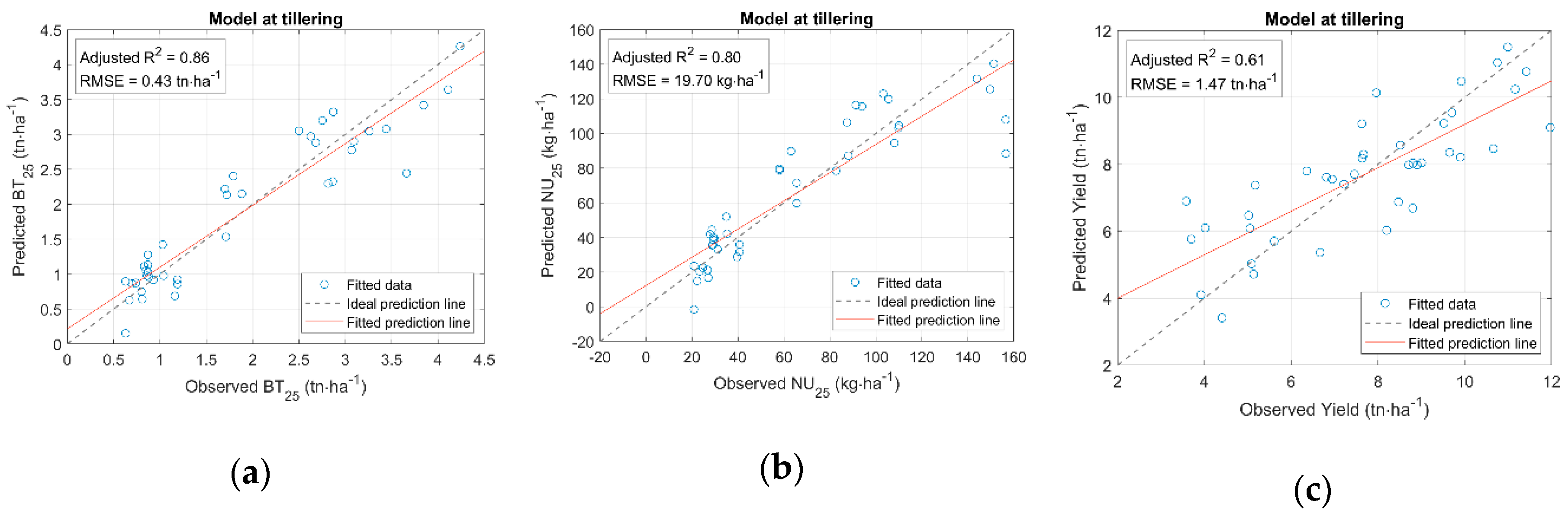
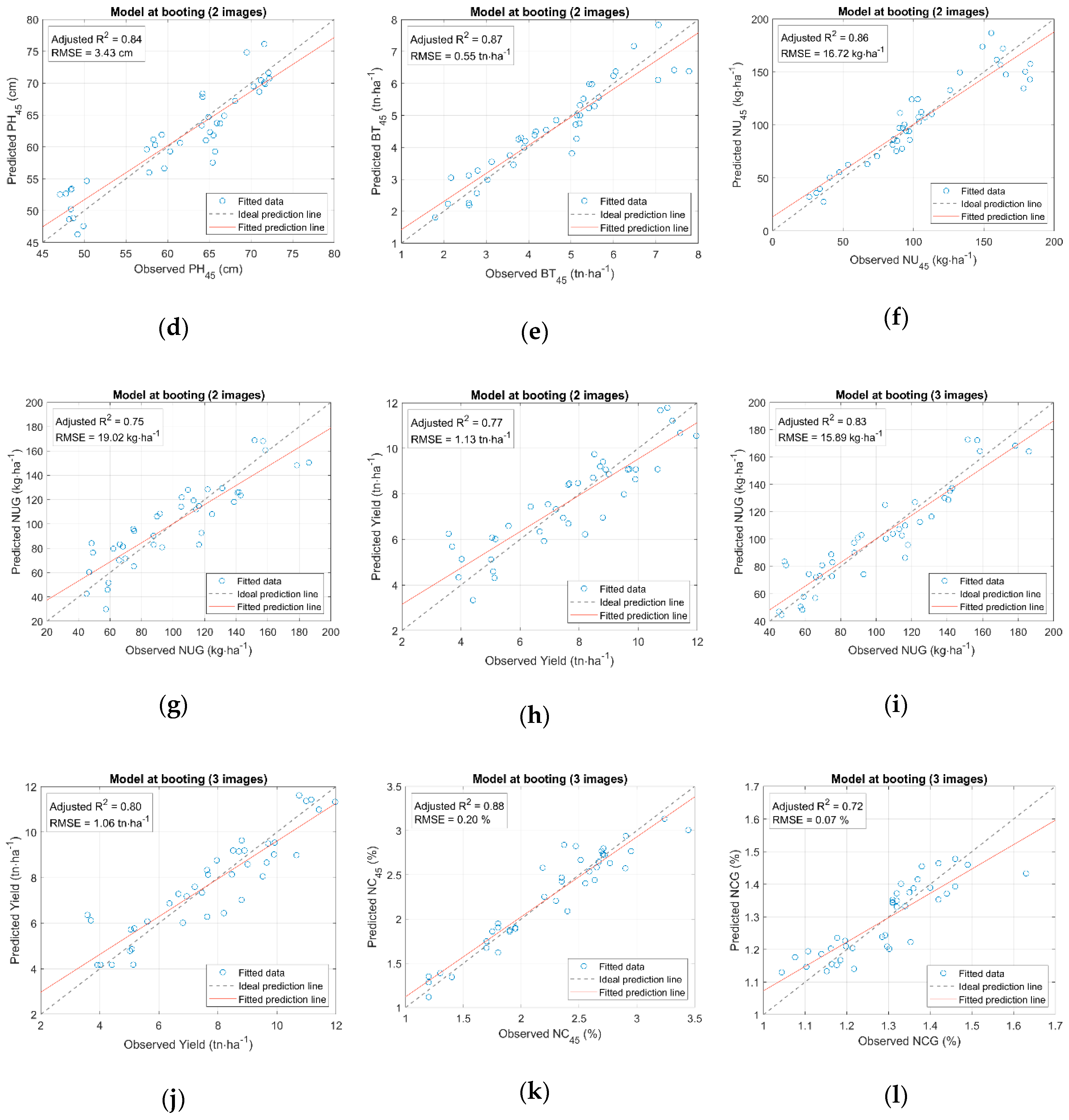
In order to give a visual representation of the models’ errors, Figure 3 depicts the scatter plots of predicted versus observed values for some indicative models constructed in each stage. The gray dashed line represents the ideal perfect linear relationship, whereas the continuous red line is the simple linear regression line of the predicted versus observed data. Models with high adjusted R² values exhibited, generally, uniform distribution of data around the ideal prediction line, with the regression line being very close to the latter and very few outliers observed in a few cases. For completeness, the scatter plots for all models constructed are provided as Supplementary Materials.

Table 7. Linear models constructed at the tillering stage, before the first top-dressing fertilization (TdF), built considering all 39 possible inputs (before input selection). G, R, RE, and NIR represent, respectively, the green, red, red-edge, and near-infrared reflectance values.

Model Formula	Adj. R2	RMSE
${\mathrm{PH}}_{25}=33.51-55.25\cdot {\mathrm{G}}_{25}$	0.12	2.59
${\mathrm{PH}}_{45}=64.07-352.2\cdot {\mathrm{R}}_{25}+8.09\cdot {\mathrm{mSR}}_{25}$	0.50	5.97
$\begin{array}{ll}{\mathrm{BT}}_{25}=& 0.50+10.09\cdot {\mathrm{G}}_{25}+0.22\cdot {\mathrm{SR}}_{25}+12.43\cdot {\mathrm{gRDVI}}_{25}-0.32\cdot {\mathrm{CI}}_{\mathrm{G},25}\\ & +1.65\cdot {\mathrm{CI}}_{\mathrm{RE},25}-11.35\cdot {\mathrm{TCARI}}_{25}-6.84\cdot \mathrm{MCARI}{1}_{25}\end{array}$	0.86	0.43
${\mathrm{BT}}_{45}=7.91-117.3\cdot {\mathrm{R}}_{25}-2.88\cdot \mathrm{MCARI}{2}_{25}+44.39\cdot {\mathrm{MTCARI}}_{25}$	0.56	1.03
${\mathrm{BT}}_{99}=25.10-263.0\cdot {\mathrm{R}}_{25}$	0.39	3.17
${\mathrm{BSL}}_{99}=12.63-167.4\cdot {\mathrm{R}}_{25}+12.57\cdot \mathrm{MCARI}{2}_{25}+64.32\cdot {\mathrm{MRETVI}}_{25}$	0.54	1.99
$\mathrm{Yield}=13.46-218.8\cdot {\mathrm{R}}_{25}-0.56\cdot {\mathrm{CI}}_{\mathrm{G},25}+11.48\cdot {\mathrm{TCARI}}_{25}+47.14\cdot {\mathrm{MTCARI}}_{25}$	0.61	1.47
$\mathrm{HI}=0.63-1.44\cdot {\mathrm{G}}_{25}$	0.24	0.05
${\mathrm{NC}}_{25}=4.01-6.43\cdot {\mathrm{G}}_{25}$	0.16	0.26
${\mathrm{NC}}_{45}=2.71-13.47\cdot {\mathrm{G}}_{25}+2.43\cdot {\mathrm{REGNDVI}}_{25}-0.45\cdot {\mathrm{MRETVI}}_{25}$	0.68	0.32
$\begin{array}{ll}{\mathrm{NC}}_{99}=& 2.70-20.81\cdot {\mathrm{G}}_{25}-5.68\cdot {\mathrm{R}}_{25}-1.35\cdot {\mathrm{CI}}_{\mathrm{G},25}+7.63\cdot \mathrm{MCARI}{2}_{25}\\ & -4.49\cdot {\mathrm{MRETVI}}_{25}\end{array}$	0.77	0.22
$\begin{array}{ll}{\mathrm{NCSL}}_{99}=& 2.12-27.46\cdot {\mathrm{R}}_{25}-0.72\cdot {\mathrm{CI}}_{\mathrm{G},25}+2.38\cdot {\mathrm{TCARI}}_{25}\\ & +1.94\cdot \mathrm{MCARI}{1}_{25}-0.59\cdot {\mathrm{MTCARI}}_{25}\end{array}$	0.70	0.28
$\mathrm{NCG}=1.52-5.52\cdot {\mathrm{R}}_{25}+0.35\cdot \mathrm{MCARI}{2}_{25}+3.86\cdot {\mathrm{MRETVI}}_{25}$	0.57	0.08
${\mathrm{NU}}_{25}=47.88-1187.6\cdot {\mathrm{G}}_{25}+1295.2\cdot {\mathrm{R}}_{25}+41.47\cdot {\mathrm{CI}}_{\mathrm{G},25}$	0.80	19.70
${\mathrm{NU}}_{45}=84.04-1610.1\cdot {\mathrm{R}}_{25}+169.9\cdot {\mathrm{NDVI}}_{25}-42.58\cdot \mathrm{TCARI}/{\mathrm{OSAVI}}_{25}$	0.50	31.88
${\mathrm{NU}}_{99}=449.1-7260.7\cdot {\mathrm{R}}_{25}-133.1\cdot {\mathrm{CI}}_{\left\{\mathrm{G},25\right\}}+752.5\cdot \mathrm{MCARI}{2}_{25}+113.6\cdot {\mathrm{MTCARI}}_{25}$	0.68	60.63
$\begin{array}{ll}{\mathrm{NUSL}}_{99}=& 273.0-4026.9\cdot {\mathrm{R}}_{25}-103.4\cdot {\mathrm{CI}}_{\mathrm{G},25}+137.1\cdot \mathrm{MCARI}{1}_{25}\\ & +263.6\cdot \mathrm{MCARI}{2}_{25}+37.87\cdot {\mathrm{MTCARI}}_{25}\end{array}$	0.68	40.20
$\begin{array}{ll}\mathrm{NUG}=& 164.8-3148.8\cdot {\mathrm{R}}_{25}+256.8\cdot {\mathrm{TCARI}}_{25}+133.7\cdot \mathrm{MCARI}{2}_{25}\\ & +52.60\cdot {\mathrm{MTCARI}}_{25}+447.1\cdot {\mathrm{MRETVI}}_{25}\end{array}$	0.58	24.79

presents the linear models constructed at the tillering stage, whereas

Table 8. Linear models constructed at the booting stage, before the second TdF, using features extracted from two UAV images (at BBCH 25 and 45), built considering all 39 possible inputs (before input selection). G, R, RE, and NIR represent, respectively, the green, red, red-edge, and near-infrared reflectance values.

Model Formula	Adj. R2	RMSE
${\mathrm{PH}}_{45}=-28.34+93.89\cdot {\mathrm{NDVI}}_{45}+29.20\cdot {\mathrm{MTCARI}}_{45}+20.43\cdot {\mathrm{NNIR}}_{45}$	0.84	3.43
${\mathrm{BT}}_{45}=-7.79+11.97\cdot {\mathrm{NDVI}}_{45}+0.96\cdot {\mathrm{mSR}}_{45}$	0.87	0.55
${\mathrm{BT}}_{99}=-7.83-91.63\cdot {\mathrm{R}}_{25}+23.35\cdot {\mathrm{NDVI}}_{45}+30.35\cdot {\mathrm{NDRE}}_{45}$	0.74	2.07
${\mathrm{BSL}}_{99}=10.52-221.1\cdot {\mathrm{R}}_{45}-1.68\cdot {\mathrm{NDVI}}_{45}+23.12\cdot {\mathrm{NDRE}}_{45}$	0.72	1.54
$\begin{array}{ll}\mathrm{Yield}=& 4.47-62.02\cdot {\mathrm{R}}_{25}-90.98\cdot {\mathrm{R}}_{45}+6.26\cdot {\mathrm{NDVI}}_{45}-0.18\cdot {\mathrm{mSR}}_{45}\\ & +18.56\cdot {\mathrm{NDRE}}_{45}\end{array}$	0.77	1.13
$\mathrm{HI}=0.39+3.80\cdot {\mathrm{R}}_{45}$	0.31	0.04
$\begin{array}{ll}{\mathrm{NC}}_{45}=& -0.97 +0.21\cdot {\mathrm{G}}_{25}-6.39\cdot {\mathrm{MTCARI}}_{25}-2.81\cdot {\mathrm{MRETVI}}_{25}+36.05\cdot {\mathrm{R}}_{45}\\ & -7.41\cdot {\mathrm{NGI}}_{45}+6.44\cdot {\mathrm{NNIR}}_{45}\end{array}$	0.88	0.20
${\mathrm{NC}}_{99}=2.55 -0.17\cdot {\mathrm{CI}}_{\mathrm{G},25}-32.92\cdot {\mathrm{R}}_{45}+2.30\cdot {\mathrm{MRETVI}}_{45}$	0.70	0.25
$\begin{array}{ll}{\mathrm{NCSL}}_{99}=& 0.39 -11.45\cdot {\mathrm{R}}_{25}+1.36\cdot {\mathrm{NDVI}}_{25}-0.87\cdot {\mathrm{CI}}_{\mathrm{G},25}+1.20\cdot \mathrm{MCARI}{1}_{25}\\ & -2.89\cdot {\mathrm{MRETVI}}_{25}-0.01\cdot {\mathrm{SR}}_{45}-0.93\cdot {\mathrm{mSR}}_{45}+6.11\cdot {\mathrm{gNDVI}}_{45}\\ & -4.49\cdot {\mathrm{gRDVI}}_{45}-2.71\cdot \mathrm{TCARI}/{\mathrm{OSAVI}}_{45}+11.90\cdot {\mathrm{NDRE}}_{45}\end{array}$	0.86	0.20
$\mathrm{NCG}=1.54+1.18\cdot {\mathrm{MRETVI}}_{25}-6.57\cdot {\mathrm{R}}_{45}+0.88\cdot {\mathrm{MRETVI}}_{45}$	0.64	0.08
${\mathrm{NU}}_{45}=-328.0+142.1\cdot {\mathrm{OSAVI}}_{45}+115.3\cdot {\mathrm{gNDVI}}_{45}+518.0\cdot {\mathrm{NNIR}}_{45}$	0.86	16.72
${\mathrm{NU}}_{99}=258.8-5637.6\cdot {\mathrm{R}}_{45}+37.94\cdot {\mathrm{mSR}}_{45}+654.4\cdot {\mathrm{MRETVI}}_{45}$	0.69	59.24
$\begin{array}{ll}{\mathrm{NCSL}}_{99}=& -2520.1 +1557.7\cdot {\mathrm{TNDVI}}_{25}-959.5\cdot {\mathrm{GWDRVI}}_{25}+25.68\cdot {\mathrm{MEVI}}_{25}\\ & -396.8\cdot {\mathrm{MRETVI}}_{25}+6817.3\cdot {\mathrm{R}}_{45}-968.7\cdot {\mathrm{DVI}}_{45}+519.9\cdot {\mathrm{gNDVI}}_{45}\\ & +98.08\cdot {\mathrm{gRDVI}}_{45}+3687.2\cdot {\mathrm{MTCARI}}_{45}-346.2\cdot {\mathrm{TCARI}/\mathrm{OSAVI}}_{45}\\ & -4979.4\cdot {\mathrm{REDVI}}_{45}+1076.2\cdot {\mathrm{NDRE}}_{45}\end{array}$	0.93	18.48
$\begin{array}{ll}\mathrm{NUG}=& 152.3-1000.2\cdot {\mathrm{R}}_{25}-2254.3\cdot {\mathrm{R}}_{45}-4.98\cdot {\mathrm{mSR}}_{45}+333.8\cdot {\mathrm{NDRE}}_{45}\\ & +25.22\cdot {\mathrm{MRETVI}}_{45}\end{array}$	0.75	19.02

and

Table 9. Linear models constructed at the booting stage, before the second TdF, using features extracted from three UAV images (at BBCH 25, 31, and 45), built considering all 39 possible inputs (before input selection). G, R, RE, and NIR represent, respectively, the green, red, red-edge, and near-infrared reflectance values.

Model Formula	Adj. R2	RMSE
${\mathrm{PH}}_{45}=-42.01+96.08\cdot {\mathrm{NDVI}}_{45}+49.09\cdot {\mathrm{NNIR}}_{45}$	0.84	3.41
${\mathrm{BT}}_{45}=-7.79+11.97\cdot {\mathrm{NDVI}}_{45}+0.96\cdot {\mathrm{mSR}}_{45}$	0.87	0.55
${\mathrm{BT}}_{99}=-7.83-91.63\cdot {\mathrm{R}}_{25}+23.35\cdot {\mathrm{NDVI}}_{45}+30.35\cdot {\mathrm{NDRE}}_{45}$	0.74	2.07
${\mathrm{BSL}}_{99}=6.73-233.7\cdot {\mathrm{R}}_{45}+6.06\cdot {\mathrm{NDVI}}_{45}-1.17\cdot {\mathrm{mSR}}_{45}+28.70\cdot {\mathrm{NDRE}}_{45}$	0.72	1.55
$\begin{array}{ll}\mathrm{Yield}=& -11.42-59.80\cdot {\mathrm{R}}_{25}+29.90\cdot {\mathrm{G}}_{31}+2.55\cdot {\mathrm{R}}_{45}+21.97\cdot {\mathrm{NDVI}}_{45}\\ & -0.77\cdot {\mathrm{mSR}}_{45}+15.74\cdot {\mathrm{NDRE}}_{45}\end{array}$	0.80	1.06
$\mathrm{HI}=0.39+3.80\cdot {\mathrm{R}}_{45}$	0.31	0.04
$\begin{array}{ll}{\mathrm{NC}}_{45}=& -6.90-4.00\cdot {\mathrm{G}}_{25}-2.50\cdot {\mathrm{G}}_{31}-5.26\cdot {\mathrm{MTCARI}}_{31}-0.57\cdot {\mathrm{REGNDVI}}_{31}\\ & +35.75\cdot {\mathrm{R}}_{45}+11.16\cdot {\mathrm{gNDVI}}_{45}+18.53\cdot {\mathrm{NGI}}_{45}\end{array}$	0.88	0.20
$\begin{array}{ll}{\mathrm{NC}}_{99}=& -0.77+6.87\cdot {\mathrm{G}}_{31}+1.40\cdot {\mathrm{TCARI}}_{31}+2.45\cdot {\mathrm{MRETVI}}_{31}+3.69\cdot {\mathrm{R}}_{45}\\ & +0.42\cdot {\mathrm{mSR}}_{45}-1.14\cdot {\mathrm{MRETVI}}_{45}\end{array}$	0.85	0.18
$\begin{array}{ll}{\mathrm{NCSL}}_{99}=& -0.60+3.21\cdot {\mathrm{G}}_{31}-0.18\cdot {\mathrm{CI}}_{\mathrm{G},31}+0.83\cdot {\mathrm{TCARI}}_{31}+0.56\cdot {\mathrm{MRETVI}}_{31}\\ & +0.35\cdot {\mathrm{mSR}}_{45}+2.00\cdot {\mathrm{NDRE}}_{45}\end{array}$	0.80	0.23
$\mathrm{NCG}=1.27+1.59\cdot {\mathrm{G}}_{31}+0.70\cdot {\mathrm{MRETVI}}_{31}-2.66\cdot {\mathrm{R}}_{45}+0.93\cdot {\mathrm{MRETVI}}_{45}$	0.72	0.07
${\mathrm{NU}}_{45}=-328.0+142.1\cdot {\mathrm{OSAVI}}_{45}+115.3\cdot {\mathrm{gNDVI}}_{45}+518.0\cdot {\mathrm{NNIR}}_{45}$	0.86	16.72
${\mathrm{NU}}_{99}=-112.3+1659.4\cdot {\mathrm{G}}_{31}-1777.8\cdot {\mathrm{R}}_{45}+73.40\cdot {\mathrm{mSR}}_{45}+281.0\cdot {\mathrm{MRETVI}}_{45}$	0.75	53.94
$\begin{array}{ll}{\mathrm{NUSL}}_{99}=& -170.1+319.2\cdot {\mathrm{G}}_{31}-51.17\cdot {\mathrm{CI}}_{\mathrm{G},31}-29.78\cdot \mathrm{TCARI}/{\mathrm{OSAVI}}_{31}\\ & +84.55\cdot {\mathrm{MRETVI}}_{31}+1922.8\cdot {\mathrm{R}}_{45}+71.83\cdot {\mathrm{mSR}}_{45}+276.9\cdot {\mathrm{NDRE}}_{45}\end{array}$	0.82	29.85
$\begin{array}{ll}\mathrm{NUG}=& -219.3-821.1\cdot {\mathrm{R}}_{25}+413.3\cdot {\mathrm{G}}_{31}+73.23\cdot {\mathrm{TCARI}}_{31}+72.67\cdot {\mathrm{MRETVI}}_{31}\\ & +569.6\cdot {\mathrm{R}}_{45}+303.7\cdot {\mathrm{NDVI}}_{45}+3.19\cdot {\mathrm{mSR}}_{45}+189.8\cdot {\mathrm{NDRE}}_{45}\end{array}$	0.83	15.89

present the models constructed at the booting stage using features extracted from two and three UAV images, respectively. For convenience, the adjusted R² and RMSE values of Table 6 are replicated in these tables as well. Focusing on the models constructed at the tillering stage that exhibit high accuracy (BT₂₅, NC₉₉, and NU₂₅ in Table 7), they mostly exploited chlorophyll-sensitive vegetation indices (gRDVI, CI_G, CI_RE, TCARI, MCARI, MRETVI) together with the green and red reflectance channels. At the BBCH 25 stage, the canopy was not fully closed, introducing strong background soil/water effects. This in turn decreased the efficiency of traditional biomass-sensitive VIs (e.g., NDVI, SR, and mSR) for estimating agronomic traits at the tillering stage. Conversely, chlorophyll-sensitive VIs incorporated the green or RE channel (or both), which rendered them more sensitive to small variations of biomass. The latter was also true for the model built for yield, although the latter exhibited relatively lower accuracy (Adj. R² = 0.61; RMSE = 1.47 tn∙ha⁻¹) than the aforementioned ones.

Regarding the models built at the booting stage (Table 8 and Table 9), models for biomass-related traits (height and biomass) tended to exploit traditional biomass-sensitive VIs such as NDVI, SR, mSR, or NDRE. Indeed, those VIs were found to exhibit high correlations with biomass in a number of vegetation monitoring studies. At the booting stage, the canopy was fully closed and those VIs could provide the necessary information for the differences in biomass, since no significant background effects were observed. The models created for yield also comprised biomass-sensitive VIs, together with the red and/or green channels. Conversely, the models built for N-related traits (NU and NC) comprised mostly VIs sensitive to chlorophyll (e.g., MTCARI, MCARI2, and TCARI/OSAVI) and VIs incorporating the green channel (e.g., CI_G and gNDVI), along with the traditional biomass-sensitive VIs in some cases. Plant N content was highly correlated with its chlorophyll content and, hence, chlorophyll-sensitive VIs increased the predictive capabilities of models for N-related traits. Moreover, the recently developed VIs [32], incorporating the RE together with the green channel, were frequently selected (most notably MRETVI and REGNDVI) for all model categories. Finally, the original green and red channels (reflectance values) were also frequently selected at both stages, which shows that the original image could increase the model’s accuracy.

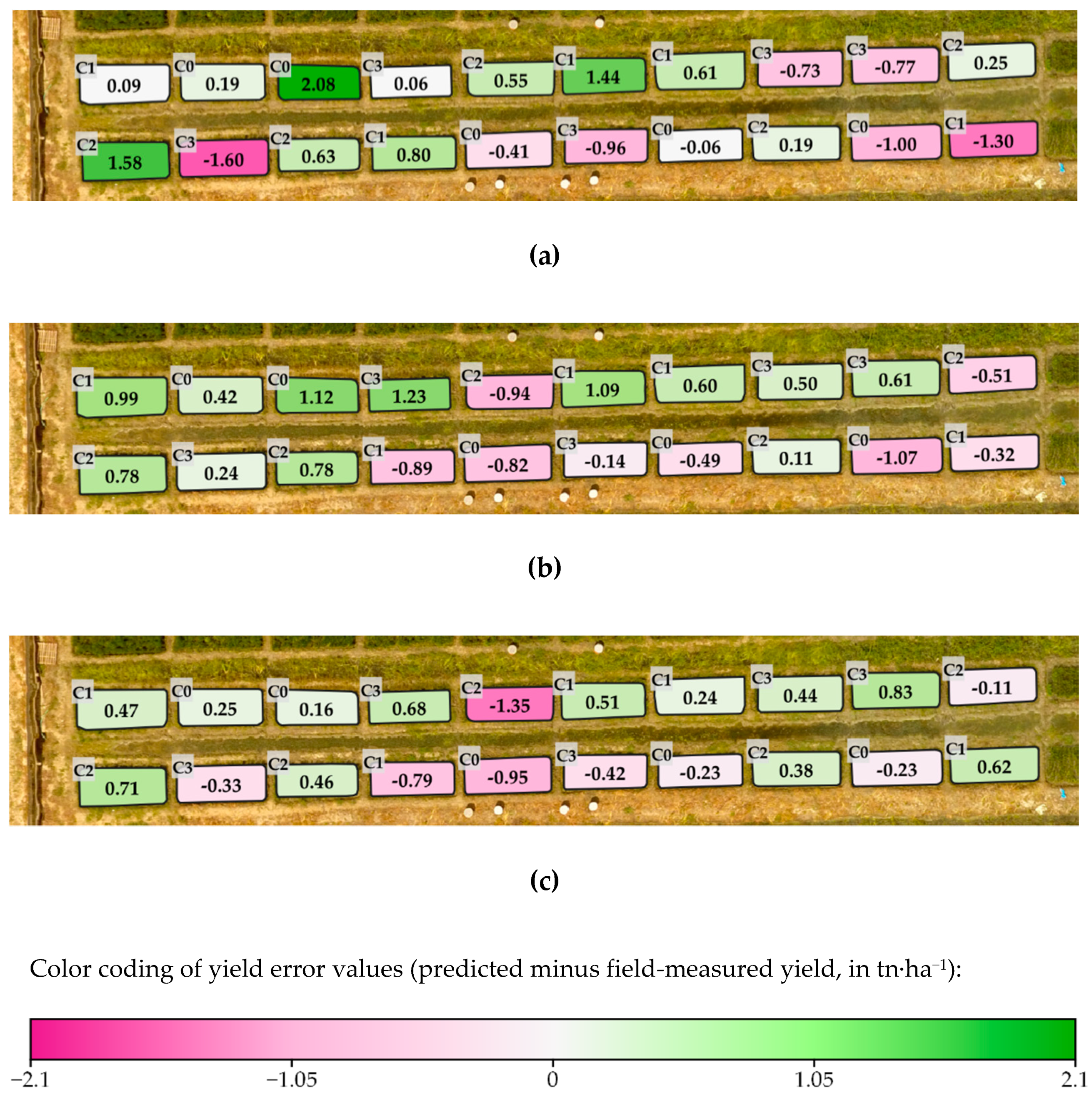
Since the agronomic traits’ estimation was performed using inputs derived from UAV imagery, the models’ output or errors could be displayed on the spatial domain, in order to support decision making. Figure 4 provides such an example, depicting each experimental plot’s yield prediction errors in 2017, for the models constructed at the tillering and the booting stage. Error values were calculated as predicted minus field-measured yield (tn∙ha⁻¹). For most plots, the errors greatly decreased (in absolute terms) from the tillering to the booting stage, as expected from the numerical results presented so far. Using three images for the models built at the booting stage further decreased the absolute errors, that is, more plots exhibited error values closer to zero. A notable exception was the top row’s fifth plot from the left, for which the absolute error increased significantly, but this was a rather isolated case. Similar maps of the models’ outputs can directly support decision making, in order to efficiently adapt the applied treatment during the growing season.

Finally,

Table 10. Summary statistics of the derived linear models, built considering the 23 possible inputs (before input selection) that do not depend on the RE channel. Adjusted coefficient of determination (R²), root mean square error (RMSE), coefficient of variation of the RMSE (CV_RMSE) (%), and number of predictors (#P) participating in each model are reported.

Trait	Models at Tillering (1 image)				Models at Booting (2 images)				Models at Booting (3 images)
	Adj. R2	RMSE	CVRMSE (%)	#P	Adj. R2	RMSE	CVRMSE (%)	#P	Adj. R2	RMSE	CVRMSE (%)	#P
PH25	0.12*	2.59	8.95	1	—	—	—	—	—	—	—	—
PH45	0.50	5.97	9.74	2	0.84	3.39	5.53	2	0.84	3.39	5.53	2
BT25	0.85	0.45	24.12	3	—	—	—	—	—	—	—	—
BT45	0.56	1.03	22.51	3	0.87	0.55	12.01	2	0.87	0.55	12.01	2
BT99	0.39	3.17	23.12	1	0.70	2.23	16.22	2	0.70	2.23	16.22	2
BSL99	0.59	1.88	24.45	4	0.69	1.61	20.99	2	0.69	1.61	20.99	2
Yield	0.61	1.48	19.19	3	0.75	1.18	15.27	4	0.79	1.08	14.04	4
HI	0.24	0.05	9.21	1	0.31	0.04	8.75	1	0.31	0.04	8.75	1
NC25	0.16	0.26	7.44	1	—	—	—	—	—	—	—	—
NC45	0.69	0.32	14.11	2	0.87	0.21	9.22	3	0.88	0.20	8.79	5
NC99	0.71	0.25	19.82	4	0.75	0.23	18.43	3	0.83	0.19	15.02	5
NCSL99	0.69	0.29	31.57	5	0.86	0.19	21.04	9	0.80	0.23	25.50	3
NCG	0.59	0.08	6.29	4	0.60	0.08	6.27	4	0.63	0.08	5.98	2
NU25	0.75	21.90	33.18	2	—	—	—	—	—	—	—	—
NU45	0.49	31.92	30.54	3	0.88	15.60	14.93	4	0.85	17.28	16.54	2
NU99	0.68	60.63	33.10	4	0.66	62.41	34.07	3	0.84	43.19	23.58	4
NUSL99	0.70	38.92	47.41	5	0.88	24.70	30.09	10	0.82	29.86	36.38	3
NUG	0.62	23.77	23.52	4	0.84	15.55	15.38	9	0.82	16.33	16.15	6

* Statistically significant at a level of 0.05; all other models are statistically significant at a level of 0.01.

reports the accuracy measures of all linear models constructed considering the 23 possible inputs (before input selection) that do not depend on the RE channel, in a similar format with Table 6 above. For some models, the accuracy measures’ values equaled those of Table 6, which was observed when the original models did not include any RE-related input. For most of the rest, their accuracy was inferior, but the difference was usually small (relative decrease in Adj. R² below 10%). This indicates that multispectral sensors without a RE channel can be used for employing the proposed methodology, with perhaps a small penalty in predictive accuracy. In a few cases, the accuracy achieved by the non-RE-dependent model was even higher than the RE-dependent ones, which is a result of the higher number of inputs selected by the lasso process for the former models. This is possible since no input selection methodology is perfect or, more precisely, lasso solves the minimization problem of equation (1), but that does not guarantee the maximization of the linear model’s accuracy built independently in a subsequent step. Nevertheless, this behavior was observed rather rarely, at least for the models that exhibit high correlations with the observed data (e.g., Adj. R² greater than 0.7). For brevity in the presentation here, the non-RE-dependent models’ formulas are provided as Supplementary Materials.

4. Discussion

Estimating N requirements and biomass-related traits in rice plants is crucial for adopting efficient precision agriculture management practices. The analysis conducted showcased that it is possible to estimate at least BT and NU at key stages within the growing season (that is, a few days before the two TdFs) using UAV-collected multispectral images and derivative VIs. At the booting stage, estimating PH, yield, and NC was also achieved with low fractions of variance unexplained. However, estimating NC before the canopy closes when the plant biomass is less compact (i.e., at tillering) is a great challenge, as observed in a number of previous studies [22,31,32,65]. Plant biomass dominates canopy reflectance before the heading stage, making the estimation of chlorophyll and N concentration at early growth stages difficult [65]. Nevertheless, an R² value of 80% was achieved for NU by the model built at tillering, which is an encouraging result. Due to the contribution of biomass and canopy structure before the heading stage and given that NU is the combination of biomass and NC, NU is more closely associated with VIs at the early growth stages [22].

Conversely, no acceptable accuracy was able to be achieved for HI at any growth stage. The improvement in HI is a consequence of increased grain population density coupled with stable individual grain weight, both of which are genotypic. Its high heritability was showcased by examining its rather weak response to variation in management practices (fertilization, population density, application of growth regulators) in the absence of severe stress [101]. Management practices that have been proposed for increasing HI of rice are based on special water treatments [102], none of which was applied in our experimentation setups. As such, no significant variations in HI across different N treatments was observed in the field data, as shown in Figure 2l.

Our modeling approach was based on multivariate linear regression exploiting several biomass- and chlorophyll-sensitive VIs, since the use of reflectance in individual bands alone has limitations due to the overlap of the effect of different nutrients and the influence of leaf and structural canopy parameters [103]. The linear regression approach in combination with lasso was selected so that the derived models are interpretable. The analysis showed that chlorophyll-sensitive VIs comprising the green and/or the RE bands are required for estimating N content at all stages and biomass at the early growth stages, whereas traditional biomass-sensitive VIs are useful for estimating biomass-relevant traits after canopy closure, which is in line with previous studies (e.g., [32,34,37]). Moreover, the reflectance values of the camera green and red bands were selected for most models at both the tillering and booting stages.

The modeling approach design tried to minimize the image acquisitions during the growing season. As such, only two images were required for estimating BT and NU a few days before each of the two TdFs. Yield prediction accuracy was higher at the booting stage (R² from 0.61 at tillering to 0.77 at booting with two images), which is consistent with a recent study [39] that showed that the best timing for predicting yield from hyperspectral measurements was indeed the booting stage. The alternative approach of using an intermediate image approximately seven to ten days after the first TdF is useful only in certain cases and, especially, if one is required to predict the plant’s N content (NU or NC) at the maturity stage. Yield prediction accuracy is also slightly increased (R² from 0.77 to 0.80) with the use of the additional image data. Nevertheless, two UAV images will be required in most real-world scenarios. It should be noted that the image acquisition stages reported here (BBCH 25, 31, and 45) are mostly indicative; the results are not expected to change if images at plus/minus one value of the BBCH scale are used instead, since the plant’s physiology changes marginally in a two–3-day period of time.

The results presented in this study can be very useful for providing N recommendations for the two TdFs in rice. One possibility is to employ the approach of Xue et al. [28], which uses the plant’s NU at each stage and the soil N supply, which can be estimated indirectly from a treatment with no N applied (C0 in our experimentation). Taking into consideration that the soil initial N supply is mandatory, since the amount of N not accounted for N recovery efficiency should not be interpreted as N that is lost without utilization from the soil–plant system. It has been reported that the recovery efficiency of N fertilizer by rice generally ranges from 20% to 80% with an average of about 30% to 40%, whereas 16% to 25% of the total applied N fertilizer could be recovered in the soil organic fraction between panicle differentiation and maturity of rice [104]. An alternative approach is to use the models’ estimations of biomass and NU or NC to calculate the plant’s N nutrition index (NNI), provided that a critical N dilution curve for the region of application and selected rice variety exists or can be calibrated [34,36,65]. A third alternative is to use the N concentration estimations derived from the models to calculate the so-called nitrogen sufficiency index (NSI), which can be directly used to provide N fertilization recommendations [105]. This approach requires the establishment of reference strips within the rice field, which receive an amount of N equal or slightly higher than that recommended by standard soil tests [106].

No matter which of the aforementioned approaches is selected for providing fertilization recommendations, the methodology presented in this study provides a cost-effective alternative to sampling approaches (either in-situ SPAD measurements or N concentration or uptake calculated in the laboratory) for estimating the rice plant’s N status. Moreover, the use of UAV-collected spatial data highlights the within-field variability of N requirements directly, since the agronomic traits estimations from the models are produced for all image pixels, thus resulting in a detail map of the whole field. The traditional approach of field sampling requires spatial interpolation between the sampled positions for obtaining equivalent maps, which generally introduces large errors in the estimations unless an unrealistically dense sampling is performed. It should be stressed that our approach does not provide any insights on the most appropriate timing to apply the TdFs. In this study we have followed the local and international standard practices for rice cultivation, with the two TdFs being performed at tillering and at booting according to the international standards. If more precision with respect to the optimal timing for applying the TdFs is required, growth simulation models that are based on meteorological predictions [107], time-series of remotely sensed data [62], or both [108] can be used.

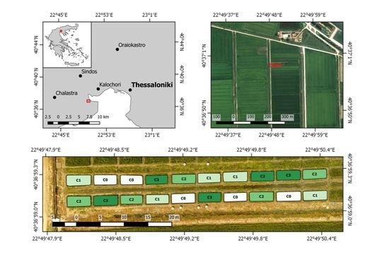
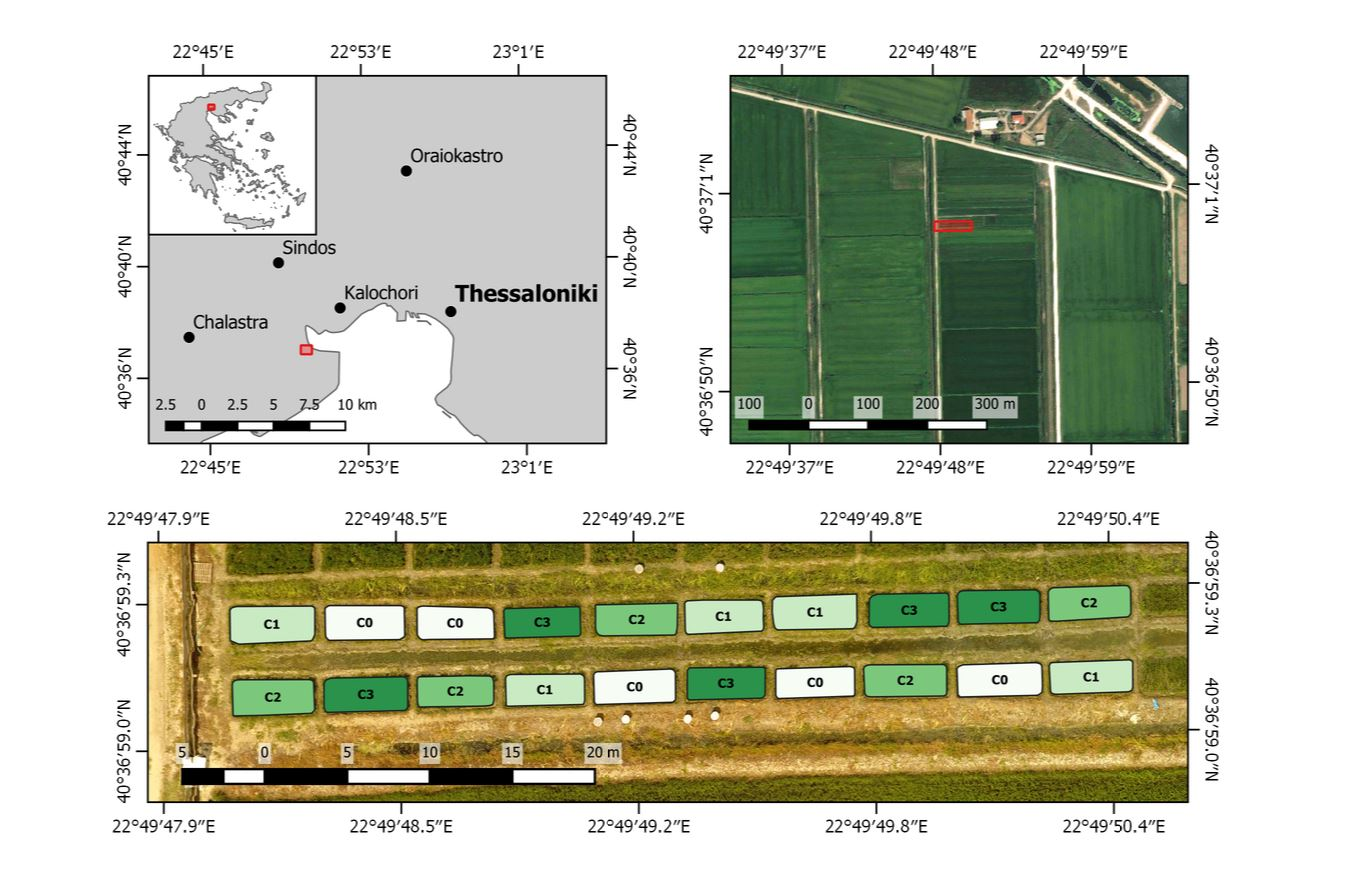
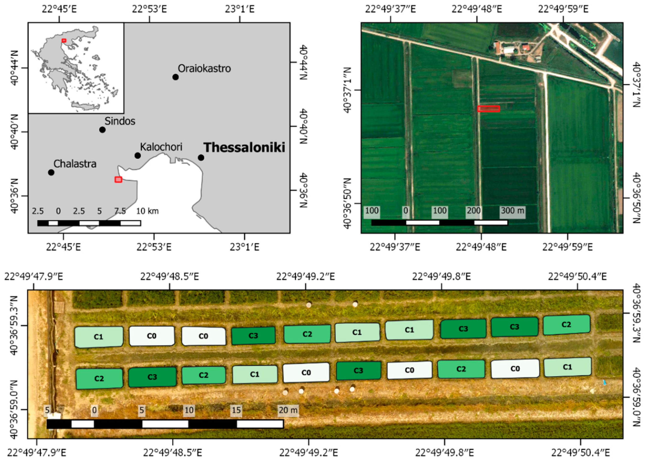
The models presented in this study were constructed considering small experimental plots, in order to facilitate field sampling and to assure that each sampling area is homogeneous, at least as much as possible. For real-world field-level applications, one has to also address the issue of accurate geo-referencing of the orthomosaic derived from the original UAV imagery. The sensitivity of global navigation satellite system (GNSS) receivers and inertial measurement units (IMU) integrated within compact sensors, such as Parrot Sequoia, will typically result in geolocation errors of 3–5 m in the orthorectified mosaic produced by most SfM software, which may be unacceptably high for precision agriculture applications, especially in smaller rice paddies. This issue can be addressed through the use of ground control points (GCPs) during image acquisition [83,109], the location of which is either fixed or measured with specialized equipment more accurate than the camera integrated one (e.g., differential GNSS). Since the latter could prove quite cumbersome and time-consuming for large-scale applications (especially in rice fields which are flooded), automatic registration methods using a reference image can be applied instead, which is an active research topic with many methods having been proposed recently [110,111,112,113]. The latter can reduce the geolocation errors to approximately 1 m or even less, which is sufficient for precision agriculture applications and variable rate fertilization in particular. From our experience, the Pix4D Mapper Pro software—that fuses SfM techniques with Sequoia’s GNSS and IMU readings during the flight and known camera/image acquisition parameters—was able to produce accurate orthomosaics in relative terms, that is, the distances between points were accurate but the whole orthomosaic exhibited shifts of 1–3 m and a very slight rotation in some cases. The subject of accurate UAV image registration is very broad and outside the scope of the current study. To this end, we actually shifted the polygons used to derive the average pixels value within each plot manually for each image, so that they corresponded to the same locations in all UAV image mosaics. Differences of a few centimeters that may have been introduced by this process are insignificant for our analysis, since the experimental plots are considered homogeneous.

For large-scale applications (big farms with scattered fields or regional level), high-resolution satellite imagery could be considered for applying our models, if UAV image acquisition is deemed to be too time or resource inefficient. For large rice fields, Sentinel-2 imagery is an obvious candidate, since it comprises a RE channel and has a short revisit cycle (five days). However, the level of analysis would be much coarser than ours, since the RE channel is provided at a spatial resolution of 20 m. Alternatively, only the 10 m bands of Sentinel-2 could be used in the analysis, employing the models built with only the 23 inputs not dependent on the RE channel (Table 10 and Tables S1–S3 in the Supplementary Materials). Commercial, very high-resolution satellite imagery is another viable alternative, at least within the framework of a commercial fertilization recommendation service provision. The models constructed with only the VIs that do not require the existence of a RE channel are useful in such a scenario, since most commercial, very high-resolution satellite sensors do not comprise an RE channel. In the latter theme, it is worth mentioning the products that have started to be offered recently by Planet (https://www.planet.com), a company that operates a large constellation of small satellites (Cubesats) that acquire daily images of the whole earth. Both PlanetScope (spatial resolution of 3 m; images acquired daily) and SkySat (spatial resolution of 0.8–1 m; sub-daily acquisitions are possible) analysis-ready data could prove useful for establishing a fertilization recommendation service based on the proposed modeling approach, since their spatial and temporal resolution is sufficient for obtaining cloud-free imagery at the required growth stages for every rice field in a broader region.

Perhaps the most important novelty of our study is the use of a cost-effective multispectral imaging sensor onboard UAVs for estimating rice agronomic traits. Most other studies for estimating rice agronomic traits employ near-ground measurements, either using hyperspectral sensors or active canopy ones, which however do not need to account for the complex background phenomena arising for the lower resolution of the UAV-collected imagery. In the latter case, techniques for removing the background [57] are difficult to be employed. This also means that the results of previous studies are not necessarily transferable to UAV-collected multispectral data. In this study we showcase that some similarities with previous results do exist, at least in terms of the most important VIs for estimating rice agronomic traits. Arguably, our study provides a more applied approach that could be integrated to any workflow or budget and can be easily adapted to a wide range of applications, even commercial ones, at least with the current technological standards.

The predictive models presented in this study were developed following field experimentation in Greece using a japonica-type rice variety. Rice in Europe is mainly cultivated in the South Mediterranean countries, which are characterized by very similar climatic conditions, whereas the cultivation treatments are also similar. Provided that no extreme variations in meteorological conditions are observed during the growing season, the results of this study should be readily applicable to other rice producing European countries, although this needs to be testified with additional experimentation in the future. Moreover, the sensor used (Parrot^® Sequoia™) was selected because it provides a generally affordable solution that is readily supported by most flight planning and orthomosaic generation software, without the need of any additional configuration on the user side. However, its bands’ spectral response is very similar with that of other alternatives or even very-high resolution satellite imagers. Therefore, our workflow could be applied considering a number of alternative sensors.

5. Conclusions

This study presented empirical models for predicting agronomic traits of rice plants through remotely-sensed multispectral imagery at key growth stages of the cultivation (at tillering and at booting). Multiple linear regression models for predicting PH, aboveground biomass, NC, ΝU, grain yield, and HI were constructed, using as input reflectance values and VIs obtained from a compact and cost-efficient four-band sensor onboard a UAV. The models were constructed using field data and images from two consecutive years in a number of experimental rice plots in Greece, employing different N treatments. The results showed that high accuracies can be achieved for NU and biomass at the tillering stage and for all traits but HI at the booting one. The proposed workflow is cost-efficient and can be easily adapted to a wide range of applications, at least with the current technological standards. To the best of our knowledge, this is the first study that presented such a comprehensive analysis for estimating various yield-related agronomic traits of rice plants during the growing season from UAV-collected multispectral data, under a flexible and easily repeatable framework.

In the future, we intend to continue the work assimilating new field data in the modeling process and assessing the performance of state-of-the-art machine learning modeling techniques. Moreover, we intend to devise N recommendation methodologies for TdFs, based on the predictions provided by the models, and assess their validity in real rice fields with precision agriculture machinery. We will also try to verify the effectiveness of our approach in other European rice producing regions. Finally, a future endeavor will be the experimentation and development of similar predictive models for indica-type rice varieties.

References

1. Global Rice Science Partnership (GRiSP). Rice Almanac, 4th ed.; International Rice Research Institute: Los Baños, Philippines, 2013; ISBN 978-971-22-0300-8. [Google Scholar]
2. Gruber, N.; Galloway, J.N. An Earth-system perspective of the global nitrogen cycle. Nature 2008, 451, 293–296. [Google Scholar] [CrossRef] [PubMed] [Green Version]
3. Seitzinger, S. Nitrogen cycle: Out of reach. Nature 2008, 452, 162–163. [Google Scholar] [CrossRef] [PubMed]
4. Liu, X.; Wang, H.; Zhou, J.; Hu, F.; Zhu, D.; Chen, Z.; Liu, Y. Effect of N Fertilization Pattern on Rice Yield, N Use Efficiency and Fertilizer–N Fate in the Yangtze River Basin, China. PLoS ONE 2016, 11, e0166002. [Google Scholar] [CrossRef] [PubMed]
5. Fageria, N.K.; Baligar, V.C. Lowland Rice Response to Nitrogen Fertilization. Commun. Soil Sci. Plant Anal. 2001, 32, 1405–1429. [Google Scholar] [CrossRef]
6. Buresh, R.J.; Garrity, D.P.; Castillo, E.G.; Chua, T.T. Fallow and Sesbania Effects on Response of Transplanted Lowland Rice to Urea. Agron. J. 1993, 85, 801–808. [Google Scholar] [CrossRef]
7. Savant, N.K.; Stangel, P.J. Deep placement of urea supergranules in transplanted rice: Principles and practices. Fertil. Res. 1990, 25, 1–83. [Google Scholar] [CrossRef]
8. Dong, H.; Li, W.; Eneji, A.E.; Zhang, D. Nitrogen rate and plant density effects on yield and late-season leaf senescence of cotton raised on a saline field. Field Crops Res. 2012, 126, 137–144. [Google Scholar] [CrossRef]
9. Rochette, P.; Angers, D.A.; Chantigny, M.H.; Gasser, M.-O.; MacDonald, J.D.; Pelster, D.E.; Bertrand, N. Ammonia Volatilization and Nitrogen Retention: How Deep to Incorporate Urea? J. Environ. Qual. 2013, 42, 1635–1642. [Google Scholar] [CrossRef] [PubMed]
10. Balafoutis, A.; Beck, B.; Fountas, S.; Vangeyte, J.; Wal, T.; van der Soto, I.; Gómez-Barbero, M.; Barnes, A.; Eory, V. Precision Agriculture Technologies Positively Contributing to GHG Emissions Mitigation, Farm Productivity and Economics. Sustainability 2017, 9, 1339. [Google Scholar] [CrossRef]
11. Yue, Q.; Ledo, A.; Cheng, K.; Albanito, F.; Lebender, U.; Sapkota, T.B.; Brentrup, F.; Stirling, C.M.; Smith, P.; Sun, J.; et al. Re-assessing nitrous oxide emissions from croplands across Mainland China. Agric. Ecosyst. Environ. 2018, 268, 70–78. [Google Scholar] [CrossRef]
12. Kritee, K.; Nair, D.; Zavala-Araiza, D.; Proville, J.; Rudek, J.; Adhya, T.K.; Loecke, T.; Esteves, T.; Balireddygari, S.; Dava, O.; et al. High nitrous oxide fluxes from rice indicate the need to manage water for both long- and short-term climate impacts. Proc. Natl. Acad. Sci. USA 2018, 115, 9720. [Google Scholar] [CrossRef] [PubMed]
13. Yan, X.; Akiyama, H. Overestimation of N2O mitigation potential by water management in rice paddy fields. Proc. Natl. Acad. Sci. USA 2018, 115, E11204–E11205. [Google Scholar] [CrossRef] [PubMed]
14. Wassmann, R.; Sander, B.O.; Yadav, S.; Bouman, B.; Singleton, G.; Stuart, A.; Hellin, J.; Johnson, D.; Hughes, J.; Butterbach-Bahl, K.; et al. New records of very high nitrous oxide fluxes from rice cannot be generalized for water management and climate impacts. Proc. Natl. Acad. Sci. USA 2019, 116, 1464–1465. [Google Scholar] [CrossRef] [PubMed]
15. Islam, S.M.M.; Gaihre, Y.K.; Shah, A.L.; Singh, U.; Sarkar, M.I.U.; Satter, M.A.; Sanabria, J.; Biswas, J.C. Rice yields and nitrogen use efficiency with different fertilizers and water management under intensive lowland rice cropping systems in Bangladesh. Nutr. Cycl. Agroecosyst. 2016, 106, 143–156. [Google Scholar] [CrossRef]
16. Macgregor, C.J.; Warren, C.R. Adopting sustainable farm management practices within a Nitrate Vulnerable Zone in Scotland: The view from the farm. Agric. Ecosyst. Environ. 2006, 113, 108–119. [Google Scholar] [CrossRef]
17. Mouratiadou, I.; Russell, G.; Topp, C.; Louhichi, K.; Moran, D. Modelling Common Agricultural Policy–Water Framework Directive interactions and cost-effectiveness of measures to reduce nitrogen pollution. Water Sci. Technol. 2010, 61, 2689–2697. [Google Scholar] [CrossRef] [PubMed]
18. Peng, S.; Cassman, K.G. Upper Threshholds of Nitrogen Uptake Rates and Associated Nitrogen Fertilizer Efficiencies in Irrigated Rice. Agron. J. 1998, 90, 178–185. [Google Scholar] [CrossRef]
19. Johnston, A.M.; Bruulsema, T.W. 4R Nutrient Stewardship for Improved Nutrient Use Efficiency. Procedia Eng. 2014, 83, 365–370. [Google Scholar] [CrossRef] [Green Version]
20. Casa, R.; Cavalieri, A.; Cascio, B.L. Nitrogen fertilisation management in precision agriculture: A preliminary application example on maize. Ital. J. Agron. 2011, 6, e5. [Google Scholar] [CrossRef]
21. Ferrero, A.; Tinarelli, A. Chapter 1—Rice Cultivation in the E.U. Ecological Conditions and Agronomical Practices. In Pesticide Risk Assessment in Rice Paddies; Capri, E., Karpouzas, D., Eds.; Elsevier: Amsterdam, The Netherlands, 2008; pp. 1–24. ISBN 978-0-444-53087-5. [Google Scholar]
22. Yu, K.; Li, F.; Gnyp, M.L.; Miao, Y.; Bareth, G.; Chen, X. Remotely detecting canopy nitrogen concentration and uptake of paddy rice in the Northeast China Plain. ISPRS J. Photogramm. Remote Sens. 2013, 78, 102–115. [Google Scholar] [CrossRef]
23. Russell, C.A.; Dunn, B.W.; Batten, G.D.; Williams, R.L.; Angus, J.F. Soil tests to predict optimum fertilizer nitrogen rate for rice. Field Crops Res. 2006, 97, 286–301. [Google Scholar] [CrossRef]
24. Gago, J.; Douthe, C.; Coopman, R.E.; Gallego, P.P.; Ribas-Carbo, M.; Flexas, J.; Escalona, J.; Medrano, H. UAVs challenge to assess water stress for sustainable agriculture. Agric. Water Manag. 2015, 153, 9–19. [Google Scholar] [CrossRef]
25. Khanal, S.; Fulton, J.; Shearer, S. An overview of current and potential applications of thermal remote sensing in precision agriculture. Comput. Electron. Agric. 2017, 139, 22–32. [Google Scholar] [CrossRef]
26. Hunt, E.R., Jr.; Daughtry, C.S.T. What good are unmanned aircraft systems for agricultural remote sensing and precision agriculture? Int. J. Remote Sens. 2018, 39, 5345–5376. [Google Scholar] [CrossRef]
27. Yang, S.; Yang, X.; Mo, J. The application of unmanned aircraft systems to plant protection in China. Precis. Agric. 2018, 19, 278–292. [Google Scholar] [CrossRef]
28. Xue, L.; Li, G.; Qin, X.; Yang, L.; Zhang, H. Topdressing nitrogen recommendation for early rice with an active sensor in south China. Precis. Agric. 2014, 15, 95–110. [Google Scholar] [CrossRef]
29. Zheng, H.; Cheng, T.; Yao, X.; Deng, X.; Tian, Y.; Cao, W.; Zhu, Y. Detection of rice phenology through time series analysis of ground-based spectral index data. Field Crops Res. 2016, 198, 131–139. [Google Scholar] [CrossRef]
30. Yao, Y.; Miao, Y.; Huang, S.; Gao, L.; Ma, X.; Zhao, G.; Jiang, R.; Chen, X.; Zhang, F.; Yu, K.; et al. Active canopy sensor-based precision N management strategy for rice. Agron. Sustain. Dev. 2012, 32, 925–933. [Google Scholar] [CrossRef] [Green Version]
31. Yao, Y.; Miao, Y.; Cao, Q.; Wang, H.; Gnyp, M.L.; Bareth, G.; Khosla, R.; Yang, W.; Liu, F.; Liu, C. In-Season Estimation of Rice Nitrogen Status with an Active Crop Canopy Sensor. IEEE J. Sel. Top. Appl. Earth Obs. Remote Sens. 2014, 7, 4403–4413. [Google Scholar] [CrossRef]
32. Cao, Q.; Miao, Y.; Wang, H.; Huang, S.; Cheng, S.; Khosla, R.; Jiang, R. Non-destructive estimation of rice plant nitrogen status with Crop Circle multispectral active canopy sensor. Field Crops Res. 2013, 154, 133–144. [Google Scholar] [CrossRef]
33. Cao, Q.; Miao, Y.; Shen, J.; Yu, W.; Yuan, F.; Cheng, S.; Huang, S.; Wang, H.; Yang, W.; Liu, F. Improving in-season estimation of rice yield potential and responsiveness to topdressing nitrogen application with Crop Circle active crop canopy sensor. Precis. Agric. 2015, 1–19. [Google Scholar] [CrossRef]
34. Lu, J.; Miao, Y.; Shi, W.; Li, J.; Yuan, F. Evaluating different approaches to non-destructive nitrogen status diagnosis of rice using portable RapidSCAN active canopy sensor. Sci. Rep. 2017, 7, 14073. [Google Scholar] [CrossRef] [PubMed] [Green Version]
35. Yang, J.; Shi, S.; Gong, W.; Du, L.; Yy, M.; Zhu, B.; Sl, S. Application of fluorescence spectrum to precisely inverse paddy rice nitrogen content. Plant Soil Environ. 2016, 61, 182–188. [Google Scholar] [CrossRef] [Green Version]
36. Huang, S.; Miao, Y.; Yuan, F.; Gnyp, M.L.; Yao, Y.; Cao, Q.; Wang, H.; Lenz-Wiedemann, V.I.S.; Bareth, G. Potential of RapidEye and WorldView-2 Satellite Data for Improving Rice Nitrogen Status Monitoring at Different Growth Stages. Remote Sens. 2017, 9, 227. [Google Scholar] [CrossRef]
37. Cheng, T.; Song, R.; Li, D.; Zhou, K.; Zheng, H.; Yao, X.; Tian, Y.; Cao, W.; Zhu, Y. Spectroscopic Estimation of Biomass in Canopy Components of Paddy Rice Using Dry Matter and Chlorophyll Indices. Remote Sens. 2017, 9, 319. [Google Scholar] [CrossRef]
38. Kanke, Y.; Tubaña, B.; Dalen, M.; Harrell, D. Evaluation of red and red-edge reflectance-based vegetation indices for rice biomass and grain yield prediction models in paddy fields. Precis. Agric. 2016, 17, 507–530. [Google Scholar] [CrossRef]
39. Kawamura, K.; Ikeura, H.; Phongchanmaixay, S.; Khanthavong, P. Canopy Hyperspectral Sensing of Paddy Fields at the Booting Stage and PLS Regression can Assess Grain Yield. Remote Sens. 2018, 10, 1249. [Google Scholar] [CrossRef]
40. Zhu, Y.; Tian, Y.; Yao, X.; Liu, X.; Cao, W. Analysis of Common Canopy Reflectance Spectra for Indicating Leaf Nitrogen Concentrations in Wheat and Rice. Plant Prod. Sci. 2007, 10, 400–411. [Google Scholar] [CrossRef] [Green Version]
41. Stroppiana, D.; Boschetti, M.; Brivio, P.A.; Bocchi, S. Plant nitrogen concentration in paddy rice from field canopy hyperspectral radiometry. Field Crops Res. 2009, 111, 119–129. [Google Scholar] [CrossRef]
42. Wang, W.; Yao, X.; Tian, Y.; Liu, X.; Ni, J.; Cao, W.; Zhu, Y. Common Spectral Bands and Optimum Vegetation Indices for Monitoring Leaf Nitrogen Accumulation in Rice and Wheat. J. Integr. Agric. 2012, 11, 2001–2012. [Google Scholar] [CrossRef]
43. Tian, Y.-C.; Gu, K.-J.; Chu, X.; Yao, X.; Cao, W.-X.; Zhu, Y. Comparison of different hyperspectral vegetation indices for canopy leaf nitrogen concentration estimation in rice. Plant Soil 2014, 376, 193–209. [Google Scholar] [CrossRef]
44. Shi, T.; Wang, J.; Liu, H.; Wu, G. Estimating leaf nitrogen concentration in heterogeneous crop plants from hyperspectral reflectance. Int. J. Remote Sens. 2015, 36, 4652–4667. [Google Scholar] [CrossRef]
45. Dunn, B.W.; Dehaan, R.; Schmidtke, L.M.; Dunn, T.S.; Meder, R. Using Field-Derived Hyperspectral Reflectance Measurement to Identify the Essential Wavelengths for Predicting Nitrogen Uptake of Rice at Panicle Initiation. J. Infrared Spectrosc. 2016, 24, 473–483. [Google Scholar] [CrossRef]
46. Moharana, S.; Dutta, S. Spatial variability of chlorophyll and nitrogen content of rice from hyperspectral imagery. ISPRS J. Photogramm. Remote Sens. 2016, 122, 17–29. [Google Scholar] [CrossRef]
47. Mahajan, G.R.; Pandey, R.N.; Sahoo, R.N.; Gupta, V.K.; Datta, S.C.; Kumar, D. Monitoring nitrogen, phosphorus and sulphur in hybrid rice (Oryza sativa L.) using hyperspectral remote sensing. Precis. Agric. 2017, 18, 736–761. [Google Scholar] [CrossRef]
48. Tan, K.; Wang, S.; Song, Y.; Liu, Y.; Gong, Z. Estimating nitrogen status of rice canopy using hyperspectral reflectance combined with BPSO-SVR in cold region. Chemom. Intell. Lab. Syst. 2018, 172, 68–79. [Google Scholar] [CrossRef]
49. Gnyp, M.L.; Miao, Y.; Yuan, F.; Ustin, S.L.; Yu, K.; Yao, Y.; Huang, S.; Bareth, G. Hyperspectral canopy sensing of paddy rice aboveground biomass at different growth stages. Field Crops Res. 2014, 155, 42–55. [Google Scholar] [CrossRef]
50. Wang, F.; Huang, J.; Lou, Z. A comparison of three methods for estimating leaf area index of paddy rice from optimal hyperspectral bands. Precis. Agric. 2011, 12, 439–447. [Google Scholar] [CrossRef]
51. Inoue, Y.; Guérif, M.; Baret, F.; Skidmore, A.; Gitelson, A.; Schlerf, M.; Darvishzadeh, R.; Olioso, A. Simple and robust methods for remote sensing of canopy chlorophyll content: A comparative analysis of hyperspectral data for different types of vegetation. Plant Cell Environ. 2016, 39, 2609–2623. [Google Scholar] [CrossRef] [PubMed]
52. Din, M.; Zheng, W.; Rashid, M.; Wang, S.; Shi, Z. Evaluating Hyperspectral Vegetation Indices for Leaf Area Index Estimation of Oryza sativa L. at Diverse Phenological Stages. Front. Plant Sci. 2017, 8, 820. [Google Scholar] [CrossRef] [PubMed]
53. Lee, Y.-J.; Yang, C.-M.; Chang, K.-W.; Shen, Y. Effects of nitrogen status on leaf anatomy, chlorophyll content and canopy reflectance of paddy rice. Bot. Stud. 2011, 52, 295–303. [Google Scholar]
54. Moharana, S.; Medhi, H.; Dutta, S. Advanced vegetation indices for sensing paddy growth via hyperspectral measurements. Geocarto Int. 2018, 33, 130–147. [Google Scholar] [CrossRef]
55. Zheng, H.; Zhou, X.; Cheng, T.; Yao, X.; Tian, Y.; Cao, W.; Zhu, Y. Evaluation of a UAV-based hyperspectral frame camera for monitoring the leaf nitrogen concentration in rice. In Proceedings of the 2016 IEEE International Geoscience and Remote Sensing Symposium (IGARSS), Beijing, China, 10–15 July 2016; pp. 7350–7353. [Google Scholar]
56. Onoyama, H.; Ryu, C.; Suguri, M.; Iida, M. Estimation of rice protein content before harvest using ground-based hyperspectral imaging and region of interest analysis. Precis. Agric. 2018, 19, 721–734. [Google Scholar] [CrossRef]
57. Zhou, K.; Deng, X.; Yao, X.; Tian, Y.; Cao, W.; Zhu, Y.; Ustin, S.L.; Cheng, T. Assessing the Spectral Properties of Sunlit and Shaded Components in Rice Canopies with Near-Ground Imaging Spectroscopy Data. Sensors 2017, 17, 578. [Google Scholar] [CrossRef] [PubMed]
58. De Bernardis, C.; Vicente-Guijalba, F.; Martinez-Marin, T.; Lopez-Sanchez, J.M. Particle Filter Approach for Real-Time Estimation of Crop Phenological States Using Time Series of NDVI Images. Remote Sens. 2016, 8, 610. [Google Scholar] [CrossRef]
59. Campos-Taberner, M.; García-Haro, F.J.; Camps-Valls, G.; Grau-Muedra, G.; Nutini, F.; Crema, A.; Boschetti, M. Multitemporal and multiresolution leaf area index retrieval for operational local rice crop monitoring. Remote Sens. Environ. 2016, 187, 102–118. [Google Scholar] [CrossRef]
60. Noureldin, N.A.; Aboelghar, M.A.; Saudy, H.S.; Ali, A.M. Rice yield forecasting models using satellite imagery in Egypt. Egypt. J. Remote Sens. Space Sci. 2013, 16, 125–131. [Google Scholar] [CrossRef] [Green Version]
61. Busetto, L.; Casteleyn, S.; Granell, C.; Pepe, M.; Barbieri, M.; Campos-Taberner, M.; Casa, R.; Collivignarelli, F.; Confalonieri, R.; Crema, A.; et al. Downstream Services for Rice Crop Monitoring in Europe: From Regional to Local Scale. IEEE J. Sel. Top. Appl. Earth Obs. Remote Sens. 2017, 10, 5423–5441. [Google Scholar] [CrossRef]
62. Yang, Z.; Shao, Y.; Li, K.; Liu, Q.; Liu, L.; Brisco, B. An improved scheme for rice phenology estimation based on time-series multispectral HJ-1A/B and polarimetric RADARSAT-2 data. Remote Sens. Environ. 2017, 195, 184–201. [Google Scholar] [CrossRef]
63. Yuzugullu, O.; Erten, E.; Hajnsek, I. Rice Growth Monitoring by Means of X-Band Co-polar SAR: Feature Clustering and BBCH Scale. IEEE Geosci. Remote Sens. Lett. 2015, 12, 1218–1222. [Google Scholar] [CrossRef]
64. Nutini, F.; Confalonieri, R.; Crema, A.; Movedi, E.; Paleari, L.; Stavrakoudis, D.; Boschetti, M. An operational workflow to assess rice nutritional status based on satellite imagery and smartphone apps. Comput. Electron. Agric. 2018, 154, 80–92. [Google Scholar] [CrossRef]
65. Huang, S.; Miao, Y.; Zhao, G.; Yuan, F.; Ma, X.; Tan, C.; Yu, W.; Gnyp, M.L.; Lenz-Wiedemann, V.I.S.; Rascher, U.; et al. Satellite Remote Sensing-Based In-Season Diagnosis of Rice Nitrogen Status in Northeast China. Remote Sens. 2015, 7, 10646–10667. [Google Scholar] [CrossRef] [Green Version]
66. Zhao, Q.; Lenz-Wiedemann, V.I.S.; Yuan, F.; Jiang, R.; Miao, Y.; Zhang, F.; Bareth, G. Investigating Within-Field Variability of Rice from High Resolution Satellite Imagery in Qixing Farm County, Northeast China. ISPRS Int. J. Geo Inf. 2015, 4, 236–261. [Google Scholar] [CrossRef] [Green Version]
67. Wang, Y.; Wang, D.; Zhang, G.; Wang, J. Estimating nitrogen status of rice using the image segmentation of G-R thresholding method. Field Crops Res. 2013, 149, 33–39. [Google Scholar] [CrossRef]
68. Li, J.; Zhang, F.; Qian, X.; Zhu, Y.; Shen, G. Quantification of rice canopy nitrogen balance index with digital imagery from unmanned aerial vehicle. Remote Sens. Lett. 2015, 6, 183–189. [Google Scholar] [CrossRef]
69. Naito, H.; Ogawa, S.; Valencia, M.O.; Mohri, H.; Urano, Y.; Hosoi, F.; Shimizu, Y.; Chavez, A.L.; Ishitani, M.; Selvaraj, M.G.; et al. Estimating rice yield related traits and quantitative trait loci analysis under different nitrogen treatments using a simple tower-based field phenotyping system with modified single-lens reflex cameras. ISPRS J. Photogramm. Remote Sens. 2017, 125, 50–62. [Google Scholar] [CrossRef]
70. Swain, K.C.; Jayasuriya, H.P.; Salokhe, V.M. Suitability of low-altitude remote sensing images for estimating nitrogen treatment variations in rice cropping for precision agriculture adoption. J. Appl. Remote Sens. 2007, 1, 013547. [Google Scholar] [CrossRef]
71. Saberioon, M.M.; Gholizadeh, A. Novel approach for estimating nitrogen content in paddy fields using low altitude remote sensing system. Int. Arch. Photogramm. Remote Sens. Spati. Inf. Sci. 2016, 41, 1011–1015. [Google Scholar] [CrossRef]
72. Xiong, D.; Chen, J.; Yu, T.; Gao, W.; Ling, X.; Li, Y.; Peng, S.; Huang, J. SPAD-based leaf nitrogen estimation is impacted by environmental factors and crop leaf characteristics. Sci. Rep. 2015, 5, 13389. [Google Scholar] [CrossRef] [PubMed] [Green Version]
73. Wakiyama, Y. The Relationship between SPAD Values and Leaf Blade Chlorophyll Content throughout the Rice Development Cycle. Jpn. Agric. Res. Q. JARQ 2016, 50, 329–334. [Google Scholar] [CrossRef] [Green Version]
74. Zhang, Y.; Su, Z.; Shen, W.; Jia, R.; Luan, J. Remote monitoring of heading rice growing and nitrogen content based on UAV images. Int. J. Smart Home 2016, 10, 103–114. [Google Scholar] [CrossRef]
75. Jinwen, L.; Jingping, Y.; Dongsheng, L.; Pinpin, F.; Tiantai, G.; Changshui, G.; Wenyue, C. Chlorophyll Meter’s Estimate of Weight-based Nitrogen Concentration in Rice Leaf is Influenced by Leaf Thickness. Plant Prod. Sci. 2011, 14, 177–183. [Google Scholar] [CrossRef] [Green Version]
76. Cabangon, R.J.; Castillo, E.G.; Tuong, T.P. Chlorophyll meter-based nitrogen management of rice grown under alternate wetting and drying irrigation. Field Crops Res. 2011, 121, 136–146. [Google Scholar] [CrossRef]
77. Wang, Y.; Wang, D.; Shi, P.; Omasa, K. Estimating rice chlorophyll content and leaf nitrogen concentration with a digital still color camera under natural light. Plant Methods 2014, 10, 36. [Google Scholar] [CrossRef] [PubMed] [Green Version]
78. Lu, J.; Miao, Y.; Huang, Y.; Shi, W.; Hu, X.; Wang, X.; Wan, J. Evaluating an unmanned aerial vehicle-based remote sensing system for estimation of rice nitrogen status. In Proceedings of the 2015 Fourth International Conference on Agro-Geoinformatics (Agro-geoinformatics), Istanbul, Turkey, 20–24 July 2015; pp. 198–203. [Google Scholar]
79. Lancashire, P.D.; Bleiholder, H.; Boom, T.V.D.; Langelüddeke, P.; Stauss, R.; Weber, E.; Witzenberger, A. A uniform decimal code for growth stages of crops and weeds. Ann. Appl. Biol. 1991, 119, 561–601. [Google Scholar] [CrossRef]
80. Growth Stages of Mono- and Dicotyledonous Plants: BBCH-Monograph; Uwe Meier, Biologische Bundesanstalt für Land- und Forstwirtschaft (Ed.) Blackwell Wissenschafts-Verlag: Berlin, Germany; Boston, MA, USA, 1997; ISBN 978-3-8263-3152-7. [Google Scholar]
81. Bremner, J.M. Total Nitrogen. In Methods of Soil Analysis. Part 2. Chemical and Microbiological Properties; Agronomy Monograph; American Society of Agronomy, Soil Science Society of America: Madison, WI, USA, 1965; pp. 1149–1178. ISBN 978-0-89118-204-7. [Google Scholar]
82. Li, X.; Yan, W.; Agrama, H.; Jia, L.; Jackson, A.; Moldenhauer, K.; Yeater, K.; McClung, A.; Wu, D. Unraveling the Complex Trait of Harvest Index with Association Mapping in Rice (Oryza sativa L.). PLoS ONE 2012, 7, e29350. [Google Scholar] [CrossRef] [PubMed]
83. Aasen, H.; Honkavaara, E.; Lucieer, A.; Zarco-Tejada, P.; Aasen, H.; Honkavaara, E.; Lucieer, A.; Zarco-Tejada, P.J. Quantitative Remote Sensing at Ultra-High Resolution with UAV Spectroscopy: A Review of Sensor Technology, Measurement Procedures, and Data Correction Workflows. Remote Sens. 2018, 10, 1091. [Google Scholar] [CrossRef]
84. Tucker, C.J. Red and photographic infrared linear combinations for monitoring vegetation. Remote Sens. Environ. 1979, 8, 127–150. [Google Scholar] [CrossRef] [Green Version]
85. Rouse, J.W., Jr.; Haas, R.H.; Schell, J.A.; Deering, D.W. Monitoring Vegetation Systems in the Great Plains with ERTS. In Third Earth Resources Technology Satellite-1 Symposium; Freden, S.C., Mercanti, E.P., Becker, M.A., Eds.; NASA Special Publication: Washington, DC, USA, 1974; Volume NASA SP-351, pp. 309–313. [Google Scholar]
86. Jordan, C.F. Derivation of Leaf-Area Index from Quality of Light on the Forest Floor. Ecology 1969, 50, 663–666. [Google Scholar] [CrossRef]
87. Chen, J.M. Evaluation of Vegetation Indices and a Modified Simple Ratio for Boreal Applications. Can. J. Remote Sens. 1996, 22, 229–242. [Google Scholar] [CrossRef]
88. Roujean, J.-L.; Breon, F.-M. Estimating PAR absorbed by vegetation from bidirectional reflectance measurements. Remote Sens. Environ. 1995, 51, 375–384. [Google Scholar] [CrossRef]
89. Huete, A.R. A soil-adjusted vegetation index (SAVI). Remote Sens. Environ. 1988, 25, 295–309. [Google Scholar] [CrossRef]
90. Rondeaux, G.; Steven, M.; Baret, F. Optimization of soil-adjusted vegetation indices. Remote Sens. Environ. 1996, 55, 95–107. [Google Scholar] [CrossRef]
91. Qi, J.; Chehbouni, A.; Huete, A.R.; Kerr, Y.H.; Sorooshian, S. A modified soil adjusted vegetation index. Remote Sens. Environ. 1994, 48, 119–126. [Google Scholar] [CrossRef]
92. Gitelson, A.A.; Kaufman, Y.J.; Merzlyak, M.N. Use of a green channel in remote sensing of global vegetation from EOS-MODIS. Remote Sens. Environ. 1996, 58, 289–298. [Google Scholar] [CrossRef]
93. Sripada, R.P.; Heiniger, R.W.; White, J.G.; Meijer, A.D. Aerial Color Infrared Photography for Determining Early In-Season Nitrogen Requirements in Corn. Agron. J. 2006, 98, 968. [Google Scholar] [CrossRef] [Green Version]
94. Gitelson, A.A.; Viña, A.; Ciganda, V.; Rundquist, D.C.; Arkebauer, T.J. Remote estimation of canopy chlorophyll content in crops. Geophys. Res. Lett. 2005, 32, L08403. [Google Scholar] [CrossRef]
95. Haboudane, D.; Miller, J.R.; Tremblay, N.; Zarco-Tejada, P.J.; Dextraze, L. Integrated narrow-band vegetation indices for prediction of crop chlorophyll content for application to precision agriculture. Remote Sens. Environ. 2002, 81, 416–426. [Google Scholar] [CrossRef]
96. Haboudane, D.; Miller, J.R.; Pattey, E.; Zarco-Tejada, P.J.; Strachan, I.B. Hyperspectral vegetation indices and novel algorithms for predicting green LAI of crop canopies: Modeling and validation in the context of precision agriculture. Remote Sens. Environ. 2004, 90, 337–352. [Google Scholar] [CrossRef]
97. Barnes, E.M.; Clarke, T.R.; Richards, S.E.; Colaizzi, P.D.; Haberland, J.; Kostrzewski, M.; Waller, P.; Choi, C.; Riley, E.; Thompson, T.; et al. Coincident detection of crop water stress, nitrogen status and canopy density using ground based multispectral data. In Proceedings of the Fifth International Conference on Precision Agriculture, Bloomington, MN, USA, 16–19 July 2000. [Google Scholar]
98. Hastie, T.; Tibshirani, R.; Friedman, J. The Elements of Statistical Learning—Data Mining, Inference, and Prediction, Springer Series in Statistics; 2nd ed.; Springer: New York, NY, USA, 2009. [Google Scholar]
99. Tibshirani, R. Regression Shrinkage and Selection via the Lasso. J. R. Stat. Soc. Ser. B Methodol. 1996, 58, 267–288. [Google Scholar] [CrossRef]
100. Milliken, G.A.; Johnson, D.E. Analysis of Messy Data Volume 1: Designed Experiments, 2nd ed.; Chapman and Hall/CRC: Boca Raton, FL, USA, 2004; ISBN 978-1-58488-334-0. [Google Scholar]
101. Hay, R.K.M. Harvest index: A review of its use in plant breeding and crop physiology. Ann. Appl. Biol. 1995, 126, 197–216. [Google Scholar] [CrossRef]
102. Yang, J.; Zhang, J. Crop management techniques to enhance harvest index in rice. J. Exp. Bot. 2010, 61, 3177–3189. [Google Scholar] [CrossRef] [PubMed] [Green Version]
103. Stroppiana, D.; Fava, F.; Boschetti, M.; Brivio, P. Estimation of Nitrogen Content in Crops and Pastures Using Hyperspectral Vegetation Indices. In Hyperspectral Remote Sensing of Vegetation; Thenkabail, P.S., Lyon, J.G., Huete, A., Eds.; CRC Press: Boca Raton, FL, USA, 2011; pp. 245–262. ISBN 978-1-4398-4537-0. [Google Scholar]
104. Bijay-Singh; Singh, V.K. Fertilizer Management in Rice. In Rice Production Worldwide; Springer: Cham, Switzerland, 2017; pp. 217–253. ISBN 978-3-319-47514-1. [Google Scholar]
105. Nigon, T.J.; Mulla, D.J.; Rosen, C.J.; Cohen, Y.; Alchanatis, V.; Knight, J.; Rud, R. Hyperspectral aerial imagery for detecting nitrogen stress in two potato cultivars. Comput. Electron. Agric. 2015, 112, 36–46. [Google Scholar] [CrossRef]
106. Peterson, T.A.; Blackmer, T.M.; Francis, D.D.; Schepers, J.S. Using a Chlorophyll Meter to Improve N Management. Hist. Mater. Univ. Neb. Linc. Ext. 1993, G93-1171, 1353. [Google Scholar]
107. Confalonieri, R.; Rosenmund, A.S.; Baruth, B. An improved model to simulate rice yield. Agron. Sustain. Dev. 2009, 29, 463–474. [Google Scholar] [CrossRef]
108. Pagani, V.; Guarneri, T.; Busetto, L.; Ranghetti, L.; Boschetti, M.; Movedi, E.; Campos-Taberner, M.; Garcia-Haro, F.J.; Katsantonis, D.; Stavrakoudis, D.; et al. A high-resolution, integrated system for rice yield forecasting at district level. Agric. Syst. 2019, 168, 181–190. [Google Scholar] [CrossRef]
109. Han, X.; Thomasson, J.A.; Bagnall, G.C.; Pugh, N.A.; Horne, D.W.; Rooney, W.L.; Jung, J.; Chang, A.; Malambo, L.; Popescu, S.C.; et al. Measurement and Calibration of Plant-Height from Fixed-Wing UAV Images. Sensors 2018, 18, 4092. [Google Scholar] [CrossRef] [PubMed]
110. Li, J.; Hu, Q.; Ai, M.; Zhong, R. Robust feature matching via support-line voting and affine-invariant ratios. ISPRS J. Photogramm. Remote Sens. 2017, 132, 61–76. [Google Scholar] [CrossRef]
111. Wei, Z.; Han, Y.; Li, M.; Yang, K.; Yang, Y.; Luo, Y.; Ong, S.-H. A Small UAV Based Multi-Temporal Image Registration for Dynamic Agricultural Terrace Monitoring. Remote Sens. 2017, 9, 904. [Google Scholar] [CrossRef]
112. Tsai, C.-H.; Lin, Y.-C. An accelerated image matching technique for UAV orthoimage registration. ISPRS J. Photogramm. Remote Sens. 2017, 128, 130–145. [Google Scholar] [CrossRef]
113. Yang, K.; Pan, A.; Yang, Y.; Zhang, S.; Ong, S.H.; Tang, H. Remote Sensing Image Registration Using Multiple Image Features. Remote Sens. 2017, 9, 581. [Google Scholar] [CrossRef]
Figure 1. Location of the experimentation station (red rectangles) in Greece (top left), overview of whole Experimental Station in Kalochori (top right), and the setup of the experimental plots (bottom). In the latter, the color of each plot denotes each treatment’s amount of nitrogen (N) applied (C0: 0 kg∙ha−1, C1: 80 kg∙ha−1, C2: 160 kg∙ha−1, and C3: 320 kg∙ha−1).
Remotesensing 11 00545 g001
Figure 2. Box plots of selected agronomic traits against the fertilization treatment: (a) BT25, (b) BT45, (c) Yield, (d) NU25, (e) N45, (f) NUG, (g) NC25, (h) NC45, (i) NUG, (j) PH25, (k) PH45, and (l) HI (see Table 1 for the description of agronomic traits).
Remotesensing 11 00545 g002
Figure 3. Scatter plots of predicted versus observed values, for selected agronomic traits. Models constructed (considering all 39 possible inputs before input selection) at tillering for (a) BT25, (b) NU25, and (c) Yield; models constructed at booting using features extracted from two unmanned aerial vehicle (UAV) images for (d) PH45, (e) BT45, (f) NU45, (g) NUG, and (h) Yield; models constructed at booting using features extracted from three UAV images for (i) NUG, (j) Yield, (k) NC45, and (l) NCG. The gray dashed line represents the ideal perfect linear relationship, whereas the continuous red line is the simple linear regression line of the predicted versus observed data.
Remotesensing 11 00545 g003aRemotesensing 11 00545 g003b
Figure 4. Yield prediction errors of each experimental plot in 2017, considering the linear models constructed at (a) the tillering stage, (b) the booting stage with two images, and (c) the booting stage with three images. Error values are expressed in tn∙ha−1 and have been calculated as predicted minus field-measured yield. The N treatment identifier is also reported for each experimental plot, following the representation of Figure 1.
Remotesensing 11 00545 g004