

On the Impacts of Historical and Future Climate Changes to the Sustainability of the Main Sardinian Forests

Dipartimento di Ingegneria Civile, Ambientale e Architettura, Università di Cagliari, 09124 Cagliari, Italy
*
Author to whom correspondence should be addressed.
Remote Sens. 2022, 14(19), 4893; https://0-doi-org.brum.beds.ac.uk/10.3390/rs14194893
Submission received: 26 July 2022
/
Revised: 26 September 2022
/
Accepted: 26 September 2022
/
Published: 30 September 2022
(This article belongs to the Special Issue Forest-Climate Interactions in a Changing Environment: Remote Sensing and In Situ Data Analysis)
Abstract
:The Mediterranean Basin is affected by climate changes that may have negative effects on forests. This study aimed to evaluate the ability of 17 forests located in the Island of Sardinia to resist or adapt to the past and future climate. Sardinia is experiencing a decreasing anthropic pressure on forests, but drought-triggered dieback in trees was recently observed and confirmed by the analysis of 20 years of satellite tree-cover data (MOD44B). Significant negative trends in yearly tree cover have affected the broad-leaved vegetation, while significative positive trends were found in the bushy sclerophyllous vegetation. Vegetation behavior resulted in being related to the mean annual precipitation (MAP); for MAP < 700 mm, we found a decline in the tall broad-leaved stands and an increase in the short ones, and the opposite was found for bushy sclerophyllous vegetations. In forests with MAP > 700 mm, both stands are stable, regardless of the growing trends in the vapor-pressure deficit (VPD) and temperature. No significative correlation between bushy sclerophyllous tree cover and the climate drivers was found, while broad-leaved tree cover is positively related to MAP1990–2019 and negatively related to the growing annual VPD. We modeled those relationships, and then we used them to coarsely predict the effects of twelve future scenarios (derived from HADGEM2-AO (CMIP5) and HadGEM3-GC31-LL (CMIP6) models) on forest tree covers. All scenarios show an annual VPD increase, and the higher its increase, the higher the trees-cover loss. The future changes in precipitation were contrasting. SC6, in line with past precipitation trends, predicts a further drop in the mean annual precipitation (−7.6%), which would correspond to an average 2.1-times-greater reduction in the tree cover (−16.09%). The future changes in precipitation for CMIP6 scenarios agree on a precipitation reduction in the range of −3.4% (SC7) to −14.29% (S12). However, although the reduction in precipitation predicted in SC12 is almost double that predicted in SC6, the consequent average reduction in TC is comparable and stands at −16%. On the contrary, SC2 predicts a turnaround with an abrupt increase of precipitation (+21.5%) in the upcoming years, with a reduction in the number of forests in water-limited areas and an increase in the percentage of tree cover in almost all forests.
1. Introduction
In recent years, a growing awareness of climate changes and related consequences has developed, and many countries are promoting mitigation and adaptation actions. However, despite this, climate changes are still taking place at an increasing rate across the globe [1,2] In the last few decades, Mediterranean countries, for example, have experienced increasing drought frequency and severity [3,4,5,6,7,8]. These findings are in line with the comparative analysis by Giorgi (2006) [9] that places the Mediterranean Basin among the most responsive regions to global climate change [10]. Future climate predictions are not encouraging, since they foresee a further air-temperature increase, particularly in the summer season, and a precipitation decrease, especially in winter [11,12].
Differences in temperature or precipitation patterns have produced a direct impact on the distribution of the terrestrial ecoregions and biomes [13]. The Mediterranean vegetation biome, for example, is characterized by the presence of shrubs (maquis) and forests, and their importance is first and foremost linked to the goods and services they provide. The Mediterranean Basin is the world’s second largest biodiversity hotspot; it is rich in plant diversity [14,15]; and it is recognized that its forests make a vital contribution to rural development, to poverty alleviation, and to food security, as well as to carbon up-take and accumulation, to controlling floods and erosion, and to sustaining biodiversity [14]. Although it has been recognized that Mediterranean forests are affected by climate change [16,17], their response to current and projected climate changes is not yet understood [1].
In many parts of the world, forested ecosystems are being transformed by both climate and land-use changes [18]. The impact of the former is more difficult to estimate when both coexist [19]. The relatively low urbanization and human activity makes the island of Sardinia, located in the middle of the Western Mediterranean Basin, an excellent reference condition for hydrological studies on past and future climate change [20,21,22,23]. Approximately half of Sardinia is covered by broadleaf forests and Mediterranean shrubs and garrigue [24], and it is the Italian region with the largest forest area. Furthermore, an extended and robust hydrological database is available in Sardinia, with almost one century of data, providing the opportunity to investigate climate change trends and their effects on forest ecosystems.
Regarding the air temperature in the Mediterranean Basin, a clear warming trend over the last four decades, for both annual and seasonal averages, is observed [25,26]. Based on the MAR1 report [27], the temperatures over land are projected to rise in the range of 0.9 to 1.5 °C or 3.7 to 5.6 °C during the 21st century for low (RCP2.6) or high greenhouse gas emissions (RCP 8.5), respectively, exceeding global mean temperature changes by 20% on an annual basis and 50% in summer, and with an increasing frequency and intensity of hot extremes [10,28]. Caloiero and Guagliardi (2020) [29] estimated an increasing trend of the Sardinian maximum monthly temperature, in the spring and summer months, for the period 1982–2011. Regarding precipitation, changes in the amounts and timing of rainfall events have been estimated in the Mediterranean regions. For instance, Feidas et al. (2007) [30], over the Greek territory, estimated a significant downward trend in annual precipitation determined by a reduction in winter precipitation, as confirmed more recently by Varlas et al. (2022) [31]. In Serbia and Montenegro, Tošić (2004) [32] analyzed the spatial and temporal variability of winter and summer precipitation at 30 rainfall stations for the period 1951–2000, finding again a decreasing trend in winter precipitation. A decreasing trend of annual precipitation was also found in Turkey [33], in the Northern Syrian Coastal Region [34], in Egypt [35], in Algeria, in Tunisia, and in Morocco [36]. A general negative trend in winter and autumn precipitation, as opposed to a positive one in spring and summer, has been found in Italy’s southern regions [37]. Montaldo and Sarigu (2017) [23] demonstrated that, in the period 1922–2011, winter precipitation in Sardinia was decreasing alarmingly, with a strong link between the winter rainfall trend and the North Atlantic Oscillation (NAO) index. The decreasing winter precipitation produced a drastic reduction of runoff, which diminished by more than 40% between 1975 and 2010 compared to the previous 1922–1974 period [23], confirming the sensitivity of island of Sardinia to climate-change effects.
Future climate scenarios by Global Climate Models (GCMs) are predicting an increase of droughts and warmer conditions in the Mediterranean Basin [11] and on the island of Sardinia [21].
From an ecological point of view, the variation in precipitation regimes and the increasing frequency of drought influence the coexistence of different biomes. Forests and savannas, for example, may be considered alternative biome states [38]. Sankaran et al. (2005) [39] found that, in Africa, a MAP of 650–700 mm is a threshold for woody cover density, which linearly increases with MAP up to 650 mm, then ceasing to be related to rainfall increase above 650, and then ceasing to 700 mm [40]. Most of the studies on this topic are focused on Africa, America, and Australia [38,39,41,42,43], while analogous research in Mediterranean regions, with a similar precipitation gradient, has not yet been seen.
Trees do not all respond in the same way to changing climates and environments, and some species are naturally resistant and resilient to climate-influenced disturbances, whereas others are sensitive and vulnerable [44,45,46]. The importance of past climate-change conditions in forest ecosystems is still under investigation [28,44,45,47], and accumulating evidence indicates that warmer temperatures and the increasing vapor-pressure deficit (VPD) are raising the mortality risks for forests during drought [48] and are negatively impacting vegetation growth [49]. Recently, Gazol and Camarero (2022) analyzed the compound effect of high summer VPD and low soil moisture on defoliation and tree mortality across European forests, highlighting that the steady increase in VPD is raising the risk of increased drought-triggered mortality rates of forests in Southern and Eastern Europe particularly.
Nowadays, long time series of optical remote-sensor observations that allow the monitoring of tree-cover dynamics are starting to be available [50,51], although not as extended as the hydrological database, and can be an appropriate support for climate-change studies. Although the observations of the Advanced Very High Resolution Radiometer (AVHRR) optical sensor started early (from 1984), they are at a coarse spatial resolution (1.1 km) that is inappropriate for heterogeneous Mediterranean ecosystems. Instead, the observations of the MODIS sensor on the Aqua and Terra satellite platforms are robust and still extended enough (from 2000), and with a more appropriate spatial resolution (250 m) [9,52,53]. In particular, a MODIS product, the MOD44B Version 6 Vegetation Continuous Fields—Collection 6 provides robust estimates of yearly tree-cover dynamics [43,54,55,56,57,58,59]
In the last decades, Sardinia has experienced long droughts that impacted the forest cover and tree density in several forests (see Supplementary Figures S2 and S3), showing alarming vulnerable conditions and raising the question of the actual and future hydrologic sustainability of the Sardinian forest ecosystems. Given this, and considering that it is well documented that MAP has a downward trend [60,61], while air temperature has a positive trend [27], in the Mediterranean Basin, we investigate the effects of climate change on the hydrological sustainability of the Sardinian forests. The specific objectives are to (1) quantify past trends in the amount, type, and distribution of tree cover in the main Sardinian forests; (2) evaluate the historical trends of the precipitation, air temperature, and vapor-pressure deficit in the Sardinian forests; and (3) evaluate the impacts of past and also future changing climate conditions on the Sardinian forest tree cover. The outcome of this study is expected to identify the key climate factors controlling tree growth and mortality in the main Sardinian forests, as well as the responses of different tree species, and therefore provide suggestions for forest management practice.
2. Methodology
2.1. Study Area
The island of Sardinia is a region of Italy located between 38°510′N and 41°150′N latitude and 8°80′E and 9°500′E longitude, with a surface of about 24,100 km2, and is second in size only to Sicily among the islands of the Mediterranean Basin (Figure 1). Sardinia has an ancient geoformation and is not earthquake prone. Its granitic basement rocks date, in fact, from the Palaeozoic and the pre-Palaeozoic Era, and they are overlain by discontinuous sedimentary and volcanic units deposited in marine or continental environments between the Permo-Carboniferous and the Quaternary [23,62]. Due to long erosion processes, the island’s highlands, formed of granite, schist, trachyte, basalt, sandstone, and dolomite limestone, range between 300 m and 1000 m. The highest peak is Punta La Marmora (1834 m), part of the Gennargentu mountain range in the center of the island. Although the island’s ranges and plateau are separated by wide alluvial valleys and flatlands (e.g., Campidano, Nurra, etc.), and although the island has an average elevation of 334 m, the slopes are so steep that most of the island is considered mountainous [62]. The climate is maritime Mediterranean, with mild, rainy winters contrasting with hot, dry summers. Two macrobioclimates (Mediterranean pluviseasonal oceanic and Temperate oceanic), one macrobioclimatic variant (Sub-Mediterranean), and four classes of continentality (from weak semihyperoceanic to weak semicontinental) can be found in Sardinia [63].
2.2. Tree Cover of the Main Sardinian Forests
Sardinia’s wildlands were selected based on the Corine Land Cover (CLC) classification produced within the framework of the Copernicus Land Monitoring Service, referring to the land cover/land use status of years 2018 and 2000 (the source dataset is described and accessible from https://land.copernicus.eu/pan-european/corine-land-cover (accessed on 1 September 2022)). This database relies on standard methodology and nomenclature with the following base parameters: 44 classes in the hierarchical 3-level CLC nomenclature, a minimum mapping unit for status layers of 25 hectares, and a minimum width of linear elements of 100 m. Among all the available classes, only the broad-leaved forests (Class ID of CLC: 3.1.1 broad-leaved forests, BLFs), the coniferous forests (Class ID of CLC 3.1.2 coniferous forests, CFs), and the bushy sclerophyllous vegetation (Class ID of CLC 3.2.3 sclerophyllous vegetation, SV) were used in this study (Table 1). These classes include only land-cover types that have not been significantly modified by human activity, and they exclude urbanized and agriculture lands. Table 1 describes the main properties of the three land-cover classes.
Tree cover was estimated from satellite information, using a product of the widely used optical MODIS sensor, the MOD44B Version 6 Vegetation Continuous Fields—Collection 6 [42,53,54,55,56,57,58]. MOD44B provides a yearly global representation of the percentage of three ground-cover components at a 250 m spatial resolution: tree-canopy coverage (TC), non-tree vegetation (NTV), and non-vegetated (bare) coverage (BS). Moreover, trees are defined as woody vegetation higher than 5 m. Data for the 2000–2019 period were used. CLC information for the years 2000 and 2018 was resampled at the 250 m spatial resolution of the MODIS product. In this study, we did not consider any pixels falling into one of the following categories: (i) nonhomogeneous land cover, (ii) land-cover change between CLC 2000 and CLC 2018, and (iii) affected by forest fires between 2000 and 2020. We selected 17 forests (Figure 1) that have been stable since 1932 [64] and included mainly tall trees with a sparse understory layer of Q. ilex subsp. Ilex, dense forests with a garrigue or maquis formation, and open woodlands of Q. ilex subsp. ballota (frequently described as savannah-like ecosystems, with low canopy cover, accompanied by grass or shrub understory). Table 2 summarizes the main properties of the forests under investigation. The forest areas range from 11.03 km2 of Su Sartu (F16) to the 447.5 km2 of the Monti del Gennargentu (F3), which is also the forest at the highest average altitude (1147 m asl).
2.3. Meteorologic Data
The rain-gauge network over Sardinia consists of 414 stations [23], and data are available for almost one century (1922–2019). We further selected 179 rain gages with more than 80 complete years of data. In more detail, 51.4% of them have ≥80 complete years of data, 86% have ≥70 complete years of data, 91.62% have ≥60 complete years of data, and 100% have more than 59 years of data.
Daily maximum and minimum air temperatures at 112 stations are available for the period 1981–2010 (39 years), but only a few of them have remained available in the last ten years, for which tree-cover data are instead available. To overcome the reduced spatial availability and density of the observed temperature data, and to extend the data set to 2019, the ERA5 monthly reanalysis dataset for the 1980–2019 period for both air temperature and dew point was used. We successfully tested the accuracy of the reanalysis dataset (correlation coefficient > 0.62, RMSE < 1.14 °C) in 6 of the observing Sardinian stations, with almost-complete datasets (Carbonia C.ra Flumentepido, Tertenia, Senorbi, Macomer, Villa Verde, Alghero, Italy).
VPD was calculated by using the ERA5 monthly near-surface air temperature (T) and dew point (Td), using the following equation [65]:
where c1 = 0.611 kPa, c2 = 17.5, and c3 = 240.978 °C. Td and T are in °C, and the resulting VPD is in kPa.
2.4. Statistical Analysis
The mean air temperature, VPD, and precipitation data were analyzed at the annual (Ty, VPDy, and Py) and seasonal scales. We used the Sardinian hydrologic year that begins on October 1 (when runoff usually resumes) and ends on September 30 of the following year (when the dry season usually ends) [21]. We distinguished the seasons as (i) ‘extended winter period’ (December through March, Tew, VPDew, and Pew); (ii) ‘shortened spring period’ (April and May, Tss, VPDss, and Pss); (iii) ‘extended summer period’ (June through September, Tes, VPDes, and Pes); and (iv) the ‘shortened fall period’ (October and November, Tsf, VPDsf, and Psf). Note that the use of the extended seasons is common in climate-change studies [21,23,66].
Trends were estimated by using the Mann–Kendall non-parametric test [67], while the slope of the linear trend was estimated with the Theil–Sen method [68,69], both of which are widely used in hydrologic applications [23,70,71,72]. To reduce the impact of autocorrelation on the statistical significance of the Mann–Kendall test and on the Theil–Sen method, different prewhitening methods are proposed by the literature [73,74,75,76]. The algorithm, proposed by Collaud et al. (2020), was used here.
The Pettitt test, a method widely used in hydrology and climate analysis [23,77,78], was used to detect the presence of a change point in the time series of the average annual precipitation over Sardinia. The spatial distribution of the MAP values observed in the rain-gauge stations over the Sardinia region was estimated through an ordinary kriging model (linear semi-variogram, 250 m resolution, and 16 neighbors). Finally, the Pearson correlation coefficient, ρ, was used for estimating the linear correlation between two datasets.
2.5. Future Projections
For future climate scenarios of precipitation and air temperature, we considered the HadGEM2-AO climate model [79] predictions from the Coupled Model Intercomparison Project Phase 5 (CMIP5), and a model coming from the following generation of HadGEM configuration, the HadGEM3-GC31-LL [80,81], from the Phase 6 (CMIP6). Montaldo and Oren (2018) showed that the HadGEM2-AO model is the one that best represents the past variations in precipitation and air temperature in Sardinia. Future climate scenarios up to 2090 were used to predict the effect of future climate change on tree cover in the forests. Following Montaldo and Oren (2018), we considered two main representative concentration pathways (RCPs) of the HadGEM2-AO model (atmospheric horizontal resolution of 1.875° × 1.25°), i.e., RCP 45 and RCP 85. In addition, two Shared Socioeconomic Pathways (SSPs) of the HadGEM3-GC31-LL model (atmospheric horizontal resolution of 1.875° × 1.25°) were considered, i.e., SSP 245 and SSP 585). The multivariate bias-correction algorithm [82], which transfers all statistical characteristics of the land-observed meteorological data to the corresponding multivariate distribution of variables simulated by the GCMs, was applied for the downscaling and bias correcting of both HadGEM2-AO and HadGEM3-GC31-LL for Sardinian forests.
3. Results
3.1. Long-Term Trends in Precipitation
Rainfall is not abundant, and on the coast, the MAP typically ranges from 415 mm (Cagliari station at 7 m asl) to 934 mm (Baunei C.ra station at 480 m asl) mm per year (Figure 2a) and follows the Mediterranean pattern, so that rainfall is concentrated in the autumn (mean value of 180 mm) and winter (mean value of 305 mm), gradually decreases during the spring (mean value of 94 mm), and hits a low in the summer (mean value of 74 mm). In inland areas, rainfall locally exceeds 700 mm per year in hilly areas and 1000 mm in the mountains (Figure 2a). Considering the full rainfall dataset (1922–2019), the mean of the island’s average annual rainfall is 729.08 mm (SD of 143.8 mm), and it varied between 469.5 mm (year 1999) and 1062 mm (year 1933). Nine of the top ten driest years that took place in this century occurred after 1980. Pettitt’s test detects a changing point in the average annual precipitation over the island in 1980. A total of 51% of the observing stations showed a significant negative trend in annual precipitation, but the spatial variability is high (Figure 3a). Limiting the rainfall dataset to the stations within close proximity of the forests analyzed, it emerges that the annual precipitation decreases significantly in almost all forests, except for F3, F4, F11, and F17, and that the βPy < −3 mm per decade in the rainfall stations is close to F5 (−3.6 mm/y at Is Cannoneris Caserma), F7 (−3.72 mm/y at Monti Mannu Caserma), F8 (−3.1 mm/y at Marrubiu, and −3.31 at Baradili), and F12 and F13 (−3.12 mm/y at Ala dei Sardi). Seasonally, precipitation decreases were largest in the winter (Figure 3b), while little and no significant changes are observed for the other seasons. The island’s average winter precipitation (Pew) was 344.47 mm (standard deviation, SD, of 98.18 mm), and it varied between 127.66 mm (year 1999) and 546.14 mm (year 1927). Even in the extended winter average precipitation, we can observe an important spatial variability, with βPew < −25 mm per decades in the rainfall stations within close proximity of F5 (−3.03 mm/y at Is Cannoneris Caserma), F7 (−2.70 mm/y at Monti Mannu Caserma), F8 (−2.43 mm/y at Marrubiu), and F13 (−2.41 mm/y at Ala dei Sardi). Variations in the Theil–Sen slope estimator of precipitation during the short spring (βPss) and the extended summer (βPes) across the island are in the range ± 0.65 mm/y, and ±1.00 mm/y for the short fall (βPsf).
The past change of the annual precipitation was well depicted in Figure 2, where the spatial variability of MAP in the island during the whole observation period (Figure 2a) and before and after the change point in 1980 was compared (Figure 2b,c). By comparing the spatial distribution of MAP in the 1922–1979 period (MAP1922–1979, 57 years; Figure 2b) with the spatial distribution of MAP in the 1980–2019 period (MAP1980–2019, 39 years; Figure 2c), it emerges that MAP is decreasing drastically in many parts of the island. In the period 1922–1979, areas with a MAP value of less than 700 mm occupied 26% of the island’s surface. This value rises to 62% in the period 1980–2019 and even includes some areas such as those in the southern part of the island and the Campidano Plain, with a MAP lower than 450 mm. At the 17 selected forests, we observed that MAP is decreasing everywhere by an average of −122.86 mm. F13 and F14 are the forests that recorded the highest (−243 mm) and the lowest (−84 mm) reduction values, respectively.
Looking at a more recent period (1990–2019, 28 hydrological years; Figure 2d)), aridity increased even more. The Theil–Sen estimator applied to the annual precipitation is negative for 54 stations, peaking above 5 mm/y for 11 stations and even above 8 mm/y for 4 stations (Marrubiu C.ra (βPy = −12.9 mm/y), Lanusei (βPy = −10.5 mm/y), Thiesi (βPy = −9.7 mm/y), and Perdasdefogu (βPy = −8.7 mm/y)). The spatial distribution of MAP in the 1990–2019 period (MAP1990–2019, 28 years; Figure 2d) showed that areas with less than 700 mm amounted to 78% of the island’s surface. In regard to the forests, two have a MAP1990–2019 <600 mm (F8 and F14), seven have a 600 mm ≤ MAP1990–2019 < 700 mm (F5, F6, F10, F11, F12, and F17), seven have a 700 mm ≤ MAP1990–2019 < 800 mm (F1, F2, F4, F7, F9, F13, and F15), and only F3 has a MAP1990–2019 of about 900 mm/y.
3.2. Trends in Tree Cover
A total of 155,518 MODIS pixels were sampled across the study area for monitoring Sardinian forests’ tree cover (Figure 1), corresponding to about 28% of the entire island. The dominant class (63.59%) is bushy sclerophyllous vegetation (BSV), while broad-leaved vegetation (BLF) accounts for 30.97%, and coniferous vegetation (CF) for just 4.51%. Regarding the 17 forests (Figure 1), in five of them (F22, F21, F20, F6, and F5) the percentage of broad-leaved vegetation is >50%, while seven forests (F23, F17, F19, F18, F16, F14, and F13) do not contain any broad-leaved vegetation (Figure 1). Bushy-sclerophyllous vegetation is present at all sites, and it dominates the other land uses in F11 (93%), F10 (73%), F14 (56%), F15 (55%), and F13 (50%). Coniferous vegetation is present in 13 of the 17 forests, but only in F12 and F18 does it exceed 20%. Due to the small number and the sparse distribution of coniferous compared to other vegetation categories, CF is not further analyzed in this paper.
The long-term trends of the percentage of tree-canopy coverage, non-tree vegetation, and bare soil over the period 2000–2019 were calculated based on MOD44B data. Figure 4 provides the spatial distribution of the Mann-Kendall τ values for both the BLF (Figure 4a–c) and BSV (Figure 4d–f) vegetation types, while Table 3 provides the average Mann-Kendall τ and the Theil-Sen slope β values of the tree-canopy coverage, non-tree vegetation, and bare soil within each of the 17 forests.
Broad-leaved forests with significant negative trends in the Mann-Kendall τ values for tree-canopy coverage are clustered mainly in the forested areas covered by this study and particularly in F5, F8, F10, and F15. Ten of the thirteen forests that contain broad-leaved vegetation show a Theil-Sen slope β ranging between −0.30% TC per year and +0.12% TC per year. Forest F5, which is the second largest forest on the island, is the one with the lowest value of Mann-Kendall τ for the tree cover canopy (τTC), equal to −0.3 (Theil-Sen slope β = −0.38%TC per year). In this forest, as in F15 the decrease in τTC contrasts with an increase in the τ of the vegetation of less than 5 m (τNTVBLF), while, for example, in F8 and F9, there was a growth in the value of bare soil (τBS). The Mann-Kendall τ of the tree-cover canopy of forests F3 and F4, which are in high elevation mountains in the central east of Sardinia, is, instead, not significant and moderately positive. The spatial distribution of trends in bushy sclerophyllous vegetation (Figure 4d–f) highlights an overall increase in treecover coverage, and a relative reduction in non-tree vegetation and non-vegetated areas. Bushy sclerophyllous vegetation in the analyzed forests shows a sensitive negative trend in τTC only in F3, and, on the contrary, 15 sites show a positive trend in τTCBSV, with βTCBSV ranging from +0.01 to +0.5% per year.
The relationship between tree canopy coverage and MAP1922–2019 for BLF and BSV was investigated year by year. As an example, Figure 5 shows the relationship of MAP1922–2019 versus tree-canopy coverage for the year 2008 for both BLF and BSV. We evaluated the breakpoint (MAPcp, identified by the regression analysis in Figure 5) at which the maximum tree cover is attained. The change in tree-canopy coverage as a function of MAP has been determined by using a 99th quantile piecewise linear regression with the identification of the breakpoint (the rainfall at which the maximum tree cover is attained), and of the maximum upper bound on tree cover (TCmax). We showed the scatter plot for the year 2008 in Figure 5 as an example because it was the year where the changing point was closest to the average value. The value of MAPcp during the 2000–2019 period was, on average, 695.3 mm (SD of 51.65 mm) for broad-leaved vegetation (between 607.47 mm (year 2002) and 759 mm (year 2019)) and 736.76 mm (SD of 48.30 mm) for bushy sclerophyllous vegetation (between 630.00 mm in the year 2004, and 810 mm in the year 2014). The maximum percentage of tree-cover canopy (TCmax) ranges from 67.08% (year 2017) to 80.30% (year 2013), with an SD of 3.38%, for broad-leaved pixels; and from 56.75 (year 2003) to 69.84% (year 2013), with a SD of 3.53%, for bushy-sclerophyllous pixels (Figure 6). There is a significant negative trend of TCmax for broad-leaved vegetation (τ = −0.47, p-value < 0.05), while for bushy sclerophyllous vegetation, the trend is not significant (τ = −0.02 and p-value = 0.92).
3.3. Long-Term Trends in Air Temperature and Vapor-Pressure Deficit
The average yearly air temperatures (Ty) in Sardinia have increased significantly by nearly 0.38 °C per decade (τ = +0.33 with p-value < 0.05) since 1990. Warming has been occurring significantly during all seasons but has been greatest during the short spring (τ = +0.33 with p-value < 0.05) and extended summer seasons (τ = +0.40 with p-value < 0.05), with a magnitude of increase of 0.48 and 0.51 °C per decade, respectively. The spatial variability of the Mann-Kendall τ values of the annual air temperature (τTy) on the island is displayed in Figure 7a. It shows an increasing trend over the entire island, with τ values ranging from 0.34 in the hilly areas of the island up to more than 0.5 in the northern and eastern part of the island and particularly close to the coastline. The Theil-Sen slope estimator (Figure 7b) reveals that Sardinia is warming on average by 0.4 °C per decade, with a gradient of increase from west (on average 0.035 °C/y) to east (on average 0.04 °C/y). Focusing on the 17 forests analyzed, all of them are subject to increasing annual and seasonal average temperatures. The maximum rises in average annual temperature are recorded in the forests located in the eastern side of the island (F9, F15, and F6, with a Theil-Sen slope estimator value of 0.52, 0.49, and 0.44 °C per decade, respectively), while by contrast, those located on the central western part of the island recorded the lowest rises (F2, F1, and F11, with a Theil-Sen slope estimator value of 0.52, 0.44, and 0.44 °C per decade, respectively). The Theil-Sen slopes (β) of the trend lines of air temperature during the short spring and extended summer are positive for all the forests, and the rise in Tss and Tes is greater than 0.05 °C/y in 15 and 7 forests, respectively.
Figure 8a,b show the spatial variability of the Theil-Sen slope estimator β on the island of the annual VPD (VPDy) and in the ‘extended summer season’ (VPDes). Overall, an increase of VPD was observed for most of the study area (Figure 8a). Increases in annual VPD have risen at a rate of approximately 0.003–0.007 kPa/y for 75% of the island, and this extrapolates to a total of 0.12 kPa for the 30-year period. The largest variations in annual VPD were in the western and northern portions of the island and the lower midsouth, while the lowest ones were in the inland hilly areas. During the extended summer season, the VPD increased over the largest areal extent of land, for which, 80% of the surface showed a Theil-Sen slope estimator in the range of 0.010–0.017 kPa/y. The most significant increases were in the mid-northern part of the island. VPD is increasing in all 17 of the forests analyzed, both annually and in every season. Increases in annual VPD have risen at a rate of approximately 0.005–0.009 kPa/y in seven forests, while for the remainder, the rate of growth is slightly lower.
3.4. Evaluation of the Climate Impact on Forest Cover Changes
We found interesting relationships between the trends of the forest tree cover and some climate drivers, in particular, the MAP1990–2019 and the Theil-Sen slope estimator of the average annual VPD (Figure 9). Correlation coefficients (Table 4) whose magnitudes are between 0.5 and 0.7 indicate variables that can be considered moderately correlated, while correlation coefficients whose magnitudes are between 0.3 and 0.5 indicate variables that can be considered only slightly correlated. The Theil-Sen slope estimator of the percentage of tree cover of broad-leaved vegetation (βTCBLF) was found to be positively correlated with MAP1990–2019 (ρ = 0.71, p-value 0.004) and negatively with βVPDy (ρ = −0.61, p-value 0.02). Opposite to this is the behavior of the Theil-Sen slope estimator of the percentage of bare soil in the analyzed broad-leaved vegetation (βBSBLF), which can be considered a measure of the forest mortality rate. βBSBLF shows a positive correlation with the annual change of annual VPD (βVPDy, ρ = 0.62, p-value 0.02) and a negative correlation with the mean annual precipitation (MAP1990–2019, ρ = −0.68, p-value 0.006). The correlations between the climatic variables analyzed and the variation in the percentage of tree cover and bare soil within the bushy sclerophyllous vegetation pixels of the forests analyzed are all low. Overall, therefore, the broad-leaved vegetation seems to be more affected by a variation in climate drivers than the bushy sclerophyllous vegetation. Figure 9 shows the scatterplots between the Theil–Sen slope estimators of the tree canopy (βTCBLF) and of the bare soil (βBSBLF) coverages and of the annual VPD(βVPDy) and MAP1990–2019 climate drivers. We fit (a) a linear function to describe the variability of βTCBLF to βVPDy (βTCBLF = −41.60 βVPDy + 0.092 (2), R2 = 0.37; Figure 8a); (b) a sigmoidal function to describe the relationship between βTCBLF and MAP1990–2019 (βTCBLF = −0.162+ 0.283/(1 + exp(−(MAP1990–2019- 750.68)/14.985); R2 = 0.81; Figure 8b); (c) a polynomial function to describe the variability of βBSBLF to βVPDy (βBSBLF= −0.136+ 24.82*βVPDy + 2124.17*βVPDy2; R2 = 0.62; Figure 8c); and (d) a linear function to describe the relationship between βBSBLF and MAP1990–2019 (βBSBLF = −0.00095 MAP1990–2019 + 0.706; R2 = 0.47; Figure 8d). All of these four relationships are significant highlighting that the warmer conditions, expressed by both an increase of vapor-pressure deficit and a decrease of precipitation, are affecting tree cover in the Sardinian forests. In Figure 9a, most of the data are close to the βTCBLF (βVPDy) linear regression line, except the F3 data, for which βTCBLF is moderately positive (but not significantly), and βVPDy is positive. Note that the F3 climate conditions are different from the other forests’ conditions because F3 is the forest at the highest elevation (Figure 1), with the lowest annual mean air temperature (~13 °C) and vapor-pressure deficit (~1.7 kPa) and the highest MAP (~900 mm). We used a sigmoidal function for βTCBLF (MAP1990–2019) relationship for fitting the F3 and F4 βTCBLF positive values, clearly related to the particularly wet conditions (MAP > 750 mm).
We used the estimated βTCBLF(βVPDy) and βTCBLF (MAP1990–2019) relationships of Figure 9 in the past for making a coarse prediction of the effects of future scenarios of precipitation and air temperature on forest tree covers.
Using the six future scenarios of the HadGEM2-AO of the CMIP5 and the six future scenarios of the HadGEM3-GC31-LL of the CMIP6 (Table 5), we estimated the future changes of tree canopy coverage (with respect to 2000–2019) in broad-leaved forests (Figure 10). All scenarios show a positive change in annual vapor-pressure deficit (Figure 10a), ranging from 4.6% in SC7 to 38.64% in SC12. A reduction in the percentage of tree cover is predicted by using the proposed βTCBLF (βVPDy) relationship for all the scenarios, ranging from 4.43% in SC7 to 38.52% in SC12 (peaking above −40% in the five forests, F3, F12, F4, F11, and F2; Figure 10c). Future changes of precipitation are predicted as both positive and negative for CMIP5 scenarios (SC1–SC6), and only negative for CMIP6 scenarios (SC7–SC12). SC6, S11, and S12 were the worst scenarios, with a reduction of 7.6%,12%, and 14.3%, which produced the maximum reduction of tree cover of 16.09%, 16.46%, and 17%, respectively (using the proposed βTCBLF (MAP1990–2019) relationship).
4. Discussion
Sardinian forests are subject to the effect of climate factors and are suffering, as demonstrated by the decrease of the canopy cover almost everywhere in recent decades. There is currently no tool to map the large-scale spatial variability and intensity of this phenomenon. This prompted us to investigate the possibility of using satellite data, and in fact, the analysis of the historical MODIS satellite data over Sardinia reveals the presence of hotspots of significant negative trends in the tree-cover percentage (Figure 4). These are mainly located in some of the forests analyzed by this study that are protected forests, not affected by fires during the period 2000–2020, and where the human impact is insignificant (no change in CLC between 2000 and 2018). The significant negative trends in the tree cover particularly affect the broad-leaved vegetation. A total of 86% of forests show a reduction in broad-leaved tree cover, and for seven forests, the Theil–Sen slope of the percentage of tree cover in broad-leaved vegetation is (βTCBLF) < 0.12%/y. The minimum value occurs in the forest of Monte Arcosu (F5), with a value of −0.30%/y, while the maximum one occurs in F3, equal to 0.12%/y (Table 4). In some forests, such as F5 and F15, the decrease in βTCBLF is contrasted by an increase in shorter vegetation, and this is confirmed by the positive values of the Theil–Sen slope of the percentage of non-tree cover in broad-leaved vegetation (βNTVBLF), while in other forests, such as F8 and F9, there is an increase in the percentage of bare soil (βBSBLF). These results agree with the drought-triggered dieback observed in some of the analyzed forests in the last decade, visible also, for instance, from a comparison of aerial photography of the F5 forest in 2009 and 2019 (Figure 2) and, in general, after the long drought of 2017 (Supplementary Figure S3). The behavior of the bushy sclerophyllous vegetation is the opposite: in 15 out of the 17 forests the Theil–Sen slope of the percentage of tree cover (βTCBSV) is positive, and it reaches the maximum value in F12, F07, and F09. These results are in line with the findings of others, who reported a reduction in woody cover along all the Mediterranean Basin [83], or in specific regions such as Spain and Italy (see Gentilesca et al. (2017) [84] for a review) and in Portugal [85]. Definitely, a main reason for which the forest is suffering is the strong decrease of precipitation in the last century in Sardinia. Using the extended Sardinian rainfall database, we performed an accurate trend analysis of Sardinian rainfall that mainly highlighted a change point (1980) in rainfall after which there was an important reduction in the percentage of surfaces with an average value of rainfall of more than 700 mm, which decreases significantly from 74% in 1922–1979 to 38% in 1980–2019, and an increase from 1 to 8 (out of 17) of the number of forests that are below the same threshold. The estimated mean annual precipitation (MAP) threshold (Sankaran et al., 2008) that limits the tree cover in semi-arid forests is 700 mm. Hence, we estimated the first reason of the forest suffering, which is the drastic decrease of the rainfall in the last century in Sardinia. Starting from this new drier condition of the Sardinian forests, we analyzed the recent period, for which more data are hopefully available, and we investigated the climate factors that are affecting forests the most. The analysis of the 20 years of historical MODIS satellite data over Sardinia reveals the presence of hotspots of significant negative trends in tree-canopy coverage. We analyzed the historical precipitation pattern over Sardinia, highlighting a significant average negative trend in the average annual precipitation (the average Mann-Kendall τ over the island is −0.2, with a p-value ≤ 0.05, and the Theil–Sen slope (βPy) is −13.81 mm per decade), which is due mainly to the negative trend of winter precipitation (average Mann-Kendall τ over the island is −0.21, with a p-value < 0.005). These alterations of the rainfall regime are a widespread phenomenon in the Mediterranean Basin [23,30,31,32,33,35,37], due to climate-change effects [35]. In Sardinia, 61% of the rainfall stations showed a significant negative trend for the average annual precipitation, but the phenomenon has a marked variability over space (Figure 3a), with a decrease of the negative trend toward the mid-eastern coast (e.g., F3 and F4 forests), as anticipated by Montaldo and Sarigu (2017), who explained that this may be caused by the combined effect of the orography and of North Atlantic Oscillation (NAO) [86]. The reduction on annual total annual precipitation caused a reduction of MAP (Figure 2), and this has been recognized as one of the factors that most influence the spatial distributions of vegetation [87]. Sankaran et al. (2008) demonstrated that, when the MAP value falls below 700 mm, the upper bound of the percentage of tree cover may be limited mainly by water availability, while above this threshold, TC has little to no dependence on rainfall. The MAP analysis over Sardinia (Figure 2), performed by this study for before and after 1980 (change point in annual precipitation estimated with Petitt’s method), highlighted an important reduction in the percentage of surfaces with an average value of rainfall of more than 700 mm, which decreases significantly from 74% in 1922–1979 to 38% in 1980–2019, and an increase from 1 to 8 (out of 17) of the number of forests that are below the same threshold (Table 3). More recently, in the period 1990–2019, the reduction in precipitation is even more marked, and in fact, in this period, 78% of the island records less than 700 mm of rainfall per year. A total of 16 out of 17 of the forests were affected by a rainfall reduction, peaking below −8.9% in F14, F13, and F8, and with F14 and F8 that dropped below the threshold of 600 mm of rainfall per year.
Having established that MAP plays a key role in determining the spatial distributions of vegetation, which is decreasing drastically in most of the island, and that this causes an increase in the number of historical forests recently located in water-limited areas (MAP < 700 mm), an attempt was made to assess the presence of any possible relationship with the spatiotemporal pattern of vegetation. The tree cover versus MAP relationships, which were found by other authors [40,42,56,88] in savanna-like ecosystems, are in line with those found in the Mediterranean context proposed by this study (Figure 5). Indeed, our data indicate a strong dependence of tree cover on rainfall below the thresholds of 695.3 ± 51.65 mm and of 736.76 ± 48.3 mm for broad-leaved and bushy sclerophyllous vegetation, respectively, while above this, there is a higher probability of witnessing a woody plant encroachment. However, looking at the maximum tree cover reached by the vegetation over time (Figure 6), we noticed that the broad-leaved vegetation is showing a 3.4% per decade reduction in TCmax, while no trend was found for bushy sclerophyllous vegetation. This means that something is reducing the ability of broad-leaved vegetation to return to its original state, and this has been recognized as an important indicator of forest degradation [89,90]. Although the analysis of the data (Figure 5) suggested that precipitation is a key driver of tree cover stability, we investigated the further main climate factors that may explain the variability of the tree cover, such as global warming and the rising vapor-pressure deficit [91].
The average yearly air temperature (Ty) is increasing alarmingly in the entire island (with Mann-Kendall τ in the range 0.23–0.47) by about 0.39 °C per decade (see Figure 7), confirming climate-change-induced temperature-rise projections [92,93]. The annual mean temperature is growing in all forests; the smallest increases in βTy are found in the forests of the mountainous areas of the hinterland (F1 and F17) and along the west coast (F7 and F8), while forests located along the east coast record the greatest positive trends (F6, F9, and F15). Summer global warming is affecting the whole island (Figure 7b) and, thus, all forests (>0.4 °C per decade), and this exacerbates the deleterious effects of leaf overheating and may affect a wide number of metabolic processes, including photosynthesis, respiration, water transport, and phenology [16]. Moreover, the increasing trend in the air temperature may aggravate the effects of drought, because temperature modulates plant water use through its effects on VPD [25,94]. A positive trend in the average annual vapor-pressure deficit has been found in the entire island (average βVPDy of about 0.05 kPa per decade), except for inland mountain areas, where the increase is moderate (i.e., F4 and F17 forests, Figure 8). The greatest increases in VPDy (βVPDy > 0.07 kPa/yr) affected the forests located in the proximity of the Campidano Plain (F14 and F8) and of the east coast of the island (F9). Plants respond to the rising vapor-pressure deficit regulating the gas exchange with the atmosphere through the closure of the stomata [94,95], and the stomatal sensitivity to the vapor-pressure deficit is highly variable across and within species [96]. The latter, such as Quercus ilex, which is the dominant species in the broad-leaved vegetation type (Figure 1), have a variable midday leaf water potential and keep their stomata open and a high photosynthetic rate for long periods, even in the presence of decreasing leaf water potential. This behavior might be beneficial when water is abundant, but under conditions of intense drought, it might endanger the plant [97]. The increase in the vapor-pressure deficit during the summer season is even greater in all forests (βVPDes = 0.007–0.015 kPa/y), making the phenomenon just described more acute and impacting plant transpiration and photosynthesis [95].
To sum up, the increasing vapor-pressure deficit substantially influences vegetation growth and forest mortality [91,98], and if high VPD conditions are combined with reduced precipitation, the risk of experiencing drought stress quickly increases [98]. Sardinia is experiencing a situation of this type. In the last three decades, on the one hand we are witnessing an increase in both average temperatures and the vapor-pressure deficit; and on the other, there is an important variation in MAP caused mainly by a drastic reduction in the winter average precipitation (see Figure 2 and Figure 3), which is important for soil water recharge and is positively correlated with tree growth [20]. The combination of those climate drivers, as found by other authors [15,99,100,101,102], may be the main cause of the shift from tall tree to shorter or no vegetation (Figure 4), and to the reduced ability of the vegetation to return to its original state (Figure 6), particularly for BLF vegetation. In closed-canopy forests, Bennett et al. (2015) [103] explain that taller trees face a more challenging hydraulic environment because they are exposed to higher solar radiation and leaf-to-air vapor-pressure deficits than those in the relatively buffered understory. This is what is most likely happening in F5, which is characterized by a MAP1922–2019 of 697 mm, which dropped to 659 mm MAP1990–2019, and growing values of temperature (τTy = 0.33) and vapor-pressure deficit (τVPDy = 0.3) and where there is a decreasing trend in broad-leaved tree canopy coverage (τTCBLF = −0.3) and a positive trend of broad-leaved non-tree vegetation coverage (τNTVBLF = +0.18). In F8, instead, the reduction in broad-leaved tree canopy coverage (τTCBLF = −0.19) is countered by an increase in bare soil (τBSBLF = +0.25). No significant trend was found in these forests for the percentage of tree cover in bushy sclerophyllous vegetation, demonstrating the greater resistance of Mediterranean maquis to climatic stresses, which is a clear step toward replacing forests with shrubland [15,104]. Areas with positive trend in the percentage of broad-leaved tree canopy coverage (F4 and F3) are mainly located in the inland mountain areas of the island, where water availability is not a problem, and the broad-leaved vegetation might benefit from the warmer weather.
The decreasing trend of broad-leaved tree canopy coverage (βTCBLF) is positively related to MAP1990–2019 (ρ = 0.71, p-value 0.004) and negatively related to the Theil–Sen slope of annual VPD (ρ = −0.61, p-value 0.02). On the contrary, the Theil–Sen slope of non-vegetated areas within broad-leaved plots (βBSBLF) shows a moderate positive correlation with the Theil–Sen slope of annual VPD (ρ = −0.62, p-value 0.01) and a negative one with MAP1990–2019 (ρ = −0.68, p-value 0.006). This means that, where we have a predominance of broad-leaved vegetation, as the average annual precipitation decreases or the annual VPD increases, the percentage of bare soil increases, while the tree cover decreases. Low or no correlation was found between bushy sclerophyllous vegetation, and the variables analyzed demonstrated low sensitivity at climate drivers. This is likely due to the fact that, drought- and heat-resistant species such as P. latifolia and Pistacia lentiscus, which are common in bushy sclerophyllous vegetation, tolerate the increase of temperature and dry conditions better than more mesic and less cold-sensitive species, such as Q. ilex [105,106].
The use of the proposed simplified βTCBLF (βVPDy) and βTCBLF (MAP1990–2019) relationships (Figure 9) estimated from past data allowed us to coarsely predict the percentage of tree cover in the future climate scenarios of the GCMs and account for variations in average annual VPD and MAP1990–2019. Six future air-temperature and precipitation scenarios were derived from the HadGEM2-AO [79] predictions of the CMIP5, identified by Montaldo and Oren (2018) as the most suitable for Sardinia, and a further six scenarios from the following generation of HadGEM configuration of CMIP6, the HadGEM3-GC31-LL predictions. We considered three time periods of increasing distance in the future and two different atmospheric CO2 concentrations (RCP 45 and RCP 85) for CMIP5, and two Shared Socioeconomic Pathways (SSP 245 and SSP 585) for CMIP6. All scenarios agree on the negative effect of the annual average VPD increase, and F2, F3, F4, F11, and F12 are the forests most affected. As expected, the higher the average annual VPD increase, the higher the tree-canopy-coverage decrease, with SC12 being the worst scenario. Future changes in precipitation were contrasting for CMIP5 scenarios; for example, SC6, in line with past precipitation trends, predicts a further drop in mean annual precipitation (−7.6%), which, based on the proposed model, would correspond to an average 2.1 times greater reduction in the tree cover (−16.09.5%). On the contrary, SC2 predicts a turnaround with an abrupt increase of precipitation (+21.5%) in the upcoming years, with a reduction in the number of forests in water-limited areas and an increase in the percentage of tree cover in almost all forests. Future changes in precipitation for CMIP6 scenarios agree on a precipitation reduction in the range of −3.4% (SC7) to −14.29% (S12). However, although the reduction in precipitation predicted in SC12 is almost double that predicted in SC6, the consequent average reduction in TC is comparable and stands at about −16%. Using the ‘Space-for-time’ substitution approach, a widely used technique to infer future trajectories of ecological systems from contemporary spatial patterns [107], we can predict a change of forest patterns in Sardinia, with more resistant tree species, such as those that compose the bushy sclerophyllous vegetation (P. latifolia, Pistacia lentiscus, Arbutus unedo, Mirtus, etc.). This already applied, for example, in a holm oak forest located in the Montserrat Mountain (Spain) [101], where, after drought-induced events of canopy die-off, there was a change in the composition and structure of the community, involving the increase in species, mostly small shrubs and herbaceous plants, as well as the arrival of non-dominant shrubs and short trees to the canopy. This approach, which follows the principles of adaptive forest management [84], can represent a valid alternative to the conservative management, based on the close-to-natural principles, that is currently required by forestry law in protected areas.
5. Conclusions
This study added evidence about the power of using satellite data for understanding the long-term tree-cover trend in forests and its relationships with climate drivers. We proposed an economic, user-friendly, and expeditious approach, which can be used by the forest management authorities in both developed and developing countries. The method allows users to map the current status of vegetation and historical trends and patterns and to identify future trajectories based on climate drivers. The results show that vegetation is responding to a warming and drier climate in different ways, as a function of species, mean annual precipitation (MAP), and vapor-pressure deficit (VPD) trends. Within broad-leaved vegetation (BLF) with a MAP lower than 700 mm, we are generally witnessing the decline of tall stands in favor of the increase of short stands, while under the same conditions, bushy sclerophyllous vegetation (BSV) showed an opposite behavior. On the contrary, within broad-leaved vegetation with a MAP higher than 700 mm, stands still have the potential to be stable even under the observed positive trends in temperature and VPD. Moreover, regardless of MAP, broad-leaved vegetation showed a drastic negative trend in TCmax (τ = −0.61 and p-value < 0.05), demonstrating that it is not able to recover its original status after the climate disturbances of the last decades. We thus believe that Sardinian broad-leaved forests, as well as others Western Mediterranean oak forests, are declining [84,85,101,108]. In general, the most negative trends in tree-canopy coverage are observed in the broad-leaved vegetation of forests located in the southern-west part of the island, where there are important historical forests composed mainly of tall trees of Quercus ilex. This finding is in line with that of other authors who demonstrate that tall trees, and in particular holm oak, are at high risk of mortality during this changing climate [99,102,103,105]. The medium- and long-term forecasts, based on future climate scenarios and on the simplified models proposed, show that the situation is destined to worsen and deserves attention. It would be useful to demonstrate the compound effects of climate variables and the uncertainties of complex climate effects to vegetation; however, such an analysis is beyond the scope of this paper, which aims only to analyze historical precipitation data in Sardinia, show the actual state of the vegetation and the connection with historical climate data, and to provide simple models that may be easily used by managers and end-users of the forests. The observed overall tree-cover trends may help to identify necessary forest-management activities within the island, whether they are close-to-natural or adaptive. If management of the second type is chosen, the positive trends in tree-canopy coverage observed in most of the bushy sclerophyllous vegetation of the forests analyzed, rather than the absence of correlation with the climate drivers investigated, would lead us to encourage the use of species falling within this category of vegetation. Moreover, it is well-known that forest-cover dynamics have a substantial impact on local water resources [58], and given that Sardinia is experiencing a drastic reduction in runoff [23], future studies should consider the compound effects of those phenomena, even under climate-change scenarios.
Supplementary Materials
The following supporting information can be downloaded at: https://0-www-mdpi-com.brum.beds.ac.uk/article/10.3390/rs14194893/s1, Figure S1. The p-value of the Mann-Kendall τ (Figure 4) of the percentage of tree cover (a), non-tree vegetation (b) and bare soil (c) for all the observed pixels classified as broad-leaved forests (BLF) and of the percentage of tree cover (c), non-tree vegetation (d) and bare soil (e) for all the observed plots classified as Bushy sclerophyllous vegetation (BSV) over the 20 years period (2000–2019). The thin black outlines indicate the 17 forests analyzed. Figure S2. Images of an observation plot (Lat 39°7.610′N, Long 8°52.80′E), located in F5, in two different periods: May 2009 and October 2019, respectively. Comparison of the two pictures makes clear the recent dieback of Quercus ilex. Figure S3. View of recent (photo taken on 24 September 2017) drought-triggered dieback at the Marganai Forest (F7, Lat. 39°20.870′N, Long. 8°34.542′E), located in the southern-west part of the island.
Author Contributions
Conceptualization and methodology S.S.C. and N.M.; software, S.S.C.; data curation, S.S.C.; writing—original draft preparation, S.S.C. and N.M.; writing—review and editing, S.S.C.; supervision, N.M.; project administration, N.M.; funding acquisition, N.M. All authors have read and agreed to the published version of the manuscript.
Funding
This work was supported by Italian Ministry of Education, University and Research (MIUR) through the SWATCH European project of the PRIMA MED program, CUP n. F24D19000010006.
Data Availability Statement
The CORINE Land Cover data are available at https://land.copernicus.eu/pan-european/corine-land-cover (accessed on 1 September 2022), the MOD44B data are available at https://appeears.earthdatacloud.nasa.gov/ (accessed on 1 September 2020), the observed data of rainfall and air temperature are available at https://www.sardegnaambiente.it/index.php?xsl=611&s=21&v=9&c=93749&na=1&n=10 (accessed on 1 September 2021), the ERA5 2 m dewpoint temperature and 2 m temperature data are available at https://cds.climate.copernicus.eu/#!/search?text=ERA5&type=dataset (accessed on 1 September 2021); and the HadGEM2-AO and the HadGEM3-GC31-LL climate model data are available at https://esgf.llnl.gov/index.html (accessed on 1 September 2021).
Acknowledgments
The authors would like to thank NASA’s Earth Science Data Systems (ESDS) program for providing MOD44B data, the European Centre for Medium-Range Weather Forecasts ECMWF for providing ERA5 2 m dewpoint temperature and 2 m temperature data, the climate modelling groups for producing and making available their model output, the Earth System Grid Federation (ESGF) for archiving the data and providing access and the multiple funding agencies who support CMIP5, CMIP6 and ESGF, and the Sardinian Regional Hydrographic Service of ARPAS, and particularly Michele Fiori, for providing rain and air-temperature data.
Conflicts of Interest
The authors declare no conflict of interest.
Nomenclature
Symbols
| BLF | broad-leaved forest |
| BS | percentage of bare soil (%) |
| BSV | bushy sclerophyllous vegetation |
| CF | coniferous forest |
| CLC | Corine Land Cover |
| CMIP5 | Coupled Model Intercomparison Project Phase 5 |
| CMIP6 | Coupled Model Intercomparison Project Phase 6 |
| GCMs | Global Climate Models |
| MAP | mean annual precipitation (mm) |
| MAPcp | MAP at which the maximum tree cover is attained (mm) |
| NTV | percentage of non-tree vegetation (%) |
| P | precipitation (mm) |
| RCP | representative concentration pathway |
| SC | future climate scenario |
| SSP | Shared Socioeconomic Pathway |
| T | near surface air temperature (°C) |
| TC | percentage of tree cover (%) |
| TCmax | maximum tree cover (%) |
| Td | dew point temperature (°C) |
| VPD | vapor-pressure deficit (kPa) |
| β | Theil–Sen slope estimator |
| τ | Mann-Kendall statistic index |
| y | annual |
| ew | ‘extended winter period’ (December through March) |
| ss | ‘shortened spring period’ (April and May) |
| es | ‘extended summer period’ (June through September) |
| sf | ‘shortened fall period’ (October and November) |
References
- Dorman, M.; Svoray, T.; Perevolotsky, A.; Moshe, Y.; Sarris, D. What Determines Tree Mortality in Dry Environments? A Multi-Perspective Approach. Ecol. Appl. 2015, 25, 1054–1071. [Google Scholar] [CrossRef] [PubMed]
- Knapp, A.K.; Hoover, D.L.; Wilcox, K.R.; Avolio, M.L.; Koerner, S.E.; La Pierre, K.J.; Loik, M.E.; Luo, Y.; Sala, O.E.; Smith, M.D. Characterizing Differences in Precipitation Regimes of Extreme Wet and Dry Years: Implications for Climate Change Experiments. Glob. Chang. Biol. 2015, 21, 2624–2633. [Google Scholar] [CrossRef]
- Briffa, K.R.; Van Der Schrier, G.; Jones, P.D. Wet and Dry Summers in Europe since 1750. Int. J. Climatol. 2009, 1905, 1894–1905. [Google Scholar] [CrossRef]
- Brunetti, M.; Maugeri, M.; Nanni, T.; Navarra, A. Droughts and Extreme Events in Regional Daily Italian Precipitation Series. Int. J. Climatol. 2002, 22, 543–558. [Google Scholar] [CrossRef]
- Ceballos, A.; Martínez-Fernández, J.; Luengo-Ugidos, M.Á. Analysis of Rainfall Trends and Dry Periods on a Pluviometric Gradient Representative of Mediterranean Climate in the Duero Basin, Spain. J. Arid Environ. 2004, 58, 215–233. [Google Scholar] [CrossRef]
- López-Moreno, J.I.; Vicente-Serrano, S.M.; Moran-Tejeda, E.; Zabalza, J.; Lorenzo-Lacruz, J.; García-Ruiz, J.M. Impact of Climate Evolution and Land Use Changes on Water Yield in the Ebro Basin. Hydrol. Earth Syst. Sci. 2011, 15, 311–322. [Google Scholar] [CrossRef]
- Martínez-Fernández, J.; Chuvieco, E.; Koutsias, N. Modelling Long-Term Fire Occurrence Factors in Spain by Accounting for Local Variations with Geographically Weighted Regression. Nat. Hazards Earth Syst. Sci. 2013, 13, 311–327. [Google Scholar] [CrossRef]
- Ventura, F.; Rossi Pisa, P.; Ardizzoni, E. Temperature and Precipitation Trends in Bologna (Italy) from 1952 to 1999. Atmos. Res. 2002, 61, 203–214. [Google Scholar] [CrossRef]
- Giorgi, F. Climate Change Hot-Spots. Geophys. Res. Lett. 2006, 33, 1–4. [Google Scholar] [CrossRef]
- Masson-Delmotte, V.; Zhai, P.; Pirani, A.; Connors, S.L.; Péan, C.; Berger, S.; Caud, N.; Chen, Y.; Goldfarb, L.; Gomis, M.I.; et al. IPCC, 2021: Climate Change 2021: The Physical Science Basis. In Contribution of Working Group I to the Sixth Assessment Report of the Intergovernmental Panel on Climate Change; Cambridge University Press: Cambridge, UK, 2021; in press. [Google Scholar]
- Ozturk, T.; Ceber, Z.P.; Türkeş, M.; Kurnaz, M.L. Projections of Climate Change in the Mediterranean Basin by Using Downscaled Global Climate Model Outputs. Int. J. Climatol. 2015, 35, 4276–4292. [Google Scholar] [CrossRef]
- Spinoni, J.; Vogt, J.V.; Naumann, G.; Barbosa, P.; Dosio, A. Will Drought Events Become More Frequent and Severe in Europe ? Int. J. Climatol. 2018, 1736, 1718–1736. [Google Scholar] [CrossRef]
- Dobrowski, S.Z.; Littlefield, C.E.; Lyons, D.S.; Hollenberg, C.; Carroll, C.; Parks, S.A.; Abatzoglou, J.T.; Hegewisch, K.; Gage, J. Protected-Area Targets Could Be Undermined by Climate Change-Driven Shifts in Ecoregions and Biomes. Commun. Earth Environ. 2021, 2, 1–11. [Google Scholar] [CrossRef]
- FAO; Plan Bleu. State of Mediterranean Forests 2018; Food and Agriculture Organization of the United Nations: Rome, Italy; Plan Bleu: Marseille, France, 2018; ISBN 978-92-5-131047-2. [Google Scholar]
- Peñuelas, J.; Sardans, J. Global Change and Forest Disturbances in the Mediterranean Basin: Breakthroughs, Knowledge Gaps, and Recommendations. Forests 2021, 12, 603. [Google Scholar] [CrossRef]
- Bussotti, F.; Ferrini, F.; Pollastrini, M.; Fini, A. The Challenge of Mediterranean Sclerophyllous Vegetation under Climate Change: From Acclimation to Adaptation. Environ. Exp. Bot. 2014, 103, 80–98. [Google Scholar] [CrossRef]
- Lindner, M.; Maroschek, M.; Netherer, S.; Kremer, A.; Barbati, A.; Garcia-Gonzalo, J.; Seidl, R.; Delzon, S.; Corona, P.; Kolström, M.; et al. Climate Change Impacts, Adaptive Capacity, and Vulnerability of European Forest Ecosystems. For. Ecol. Manag. 2010, 259, 698–709. [Google Scholar] [CrossRef]
- Allen, C.D.; Macalady, A.K.; Chenchouni, H.; Bachelet, D.; McDowell, N.; Vennetier, M.; Kitzberger, T.; Rigling, A.; Breshears, D.D.; Hogg, E.H.; et al. A Global Overview of Drought and Heat-Induced Tree Mortality Reveals Emerging Climate Change Risks for Forests. For. Ecol. Manag. 2010, 259, 660–684. [Google Scholar] [CrossRef]
- Tomer, M.D.; Schilling, K.E. A Simple Approach to Distinguish Land-Use and Climate-Change Effects on Watershed Hydrology. J. Hydrol. 2009, 376, 24–33. [Google Scholar] [CrossRef]
- Montaldo, N.; Corona, R.; Curreli, M.; Sirigu, S.; Piroddi, L.; Oren, R. Rock Water as a Key Resource for Patchy Ecosystems on Shallow Soils: Digging Deep Tree Clumps Subsidize Surrounding Surficial Grass. Earth’s Future 2021, 9, 1–24. [Google Scholar] [CrossRef]
- Montaldo, N.; Oren, R. Changing Seasonal Rainfall Distribution With Climate Directs Contrasting Impacts at Evapotranspiration and Water Yield in the Western Mediterranean Region. Earth’s Future 2018, 6, 841–856. [Google Scholar] [CrossRef]
- Piras, M.; Mascaro, G.; Deidda, R.; Vivoni, E.R. Impacts of Climate Change on Precipitation and Discharge Extremes through the Use of Statistical Downscaling Approaches in a Mediterranean Basin. Sci. Total Environ. 2016, 543, 952–964. [Google Scholar] [CrossRef]
- Montaldo, N.; Sarigu, A. Potential Links between the North Atlantic Oscillation and Decreasing Precipitation and Runoff on a Mediterranean Area. J. Hydrol. 2017, 553, 419–437. [Google Scholar] [CrossRef]
- Salis, M.; Ager, A.A.; Alcasena, F.J.; Arca, B.; Finney, M.A.; Pellizzaro, G.; Spano, D. Analyzing Seasonal Patterns of Wildfire Exposure Factors in Sardinia, Italy. Environ. Monit. Assess. 2015, 187, 4175. [Google Scholar] [CrossRef] [PubMed]
- Gazol, A.; Camarero, J.J. Compound Climate Events Increase Tree Drought Mortality across European Forests. Sci. Total Environ. 2022, 816, 151604. [Google Scholar] [CrossRef]
- Lionello, P.; Abrantes, F.; Congedi, L.; Dulac, F.; Gacic, M.; Gomis, D.; Goodess, C.; Hoff, H.; Kutiel, H.; Luterbacher, J.; et al. Introduction: Mediterranean Climate-Background Information. In The Climate of the Mediterranean Region; Lionello, P., Ed.; Elsevier: Amsterdam, The Netherlands, 2012; pp. xxxv–xc. ISBN 9780124160422. [Google Scholar]
- Cramer, W.; Guiot, J.; Marini, K.; Azzopardi, B.; Balzan, M.V.; Cherif, S.; Doblas-Miranda, E.; dos Santos, M.; Drobinski, P.; Fader, M.; et al. MedECC 2020 Summary for Policymakers. In Climate and Environmental Change in the Mediterranean Basin—Current Situation and Risks for the Future. First Mediterranean Assessment Report; Cramer, W., Guiot, J., Marini, K., Eds.; Union for the Mediterranean, Plan Bleu, UNEP: Marseille, France, 2020; pp. 11–40. [Google Scholar]
- Camarero, J.J.; Gazol, A.; Sangüesa-Barreda, G.; Cantero, A.; Sánchez-Salguero, R.; Sánchez-Miranda, A.; Granda, E.; Serra-Maluquer, X.; Ibáñez, R. Forest Growth Responses to Drought at Short- and Long-Term Scales in Spain: Squeezing the Stress Memory from Tree Rings. Front. Ecol. Evol. 2018, 6, 9. [Google Scholar] [CrossRef]
- Caloiero, T.; Guagliardi, I. Temporal Variability of Temperature Extremes in the Sardinia Region (Italy). Hydrology 2020, 7, 55. [Google Scholar] [CrossRef]
- Feidas, H.; Noulopoulou, C.; Makrogiannis, T.; Bora-Senta, E. Trend Analysis of Precipitation Time Series in Greece and Their Relationship with Circulation Using Surface and Satellite Data: 1955–2001. Theor. Appl. Climatol. 2007, 87, 155–177. [Google Scholar] [CrossRef]
- Varlas, G.; Stefanidis, K.; Papaioannou, G.; Panagopoulos, Y.; Pytharoulis, I.; Katsafados, P.; Papadopoulos, A.; Dimitriou, E. Unravelling Precipitation Trends in Greece since 1950s Using ERA5 Climate Reanalysis Data. Climate 2022, 10, 12. [Google Scholar] [CrossRef]
- Tošić, I.A. Spatial and Temporal Variability of Winter and Summer Precipitation over Serbia and Montenegro. Theor. Appl. Climatol. 2004, 77, 47–56. [Google Scholar] [CrossRef]
- Unal, Y.S.; Deniz, A.; Toros, H.; Incecik, S. Temporal and Spatial Patterns of Precipitation Variability for Annual, Wet, and Dry Seasons in Turkey. Int. J. Climatol. 2012, 32, 392–405. [Google Scholar] [CrossRef]
- Salameh, A.A.M.; Fallah, R.Q. Changes in Air Temperature and Precipitation over the Syrian Coastal Region (Lattakia Governorate) from 1970 to 2016. Cuad. Geogr. 2018, 57, 140–151. [Google Scholar] [CrossRef]
- Gado, T.A.; El-Hagrsy, R.M.; Rashwan, I.M.H. Spatial and Temporal Rainfall Changes in Egypt. Environ. Sci. Pollut. Res. 2019, 26, 28228–28242. [Google Scholar] [CrossRef] [PubMed]
- Tramblay, Y.; El Adlouni, S.; Servat, E. Trends and Variability in Extreme Precipitation Indices over Maghreb Countries. Nat. Hazards Earth Syst. Sci. 2013, 13, 3235–3248. [Google Scholar] [CrossRef]
- Scorzini, A.R.; Leopardi, M. Precipitation and Temperature Trends over Central Italy (Abruzzo Region): 1951–2012. Theor. Appl. Climatol. 2019, 135, 959–977. [Google Scholar] [CrossRef]
- Staver, A.C.; Archibald, S.; Levin, S.A. The Global Extent and Determinants of Savanna and Forest as Alternative Biome States. Science 2011, 334, 230–232. [Google Scholar] [CrossRef]
- Sankaran, M.; Hanan, N.P.; Scholes, R.J.; Ratnam, J.; Augustine, D.J.; Cade, B.S.; Gignoux, J.; Higgins, S.I.; Le Roux, X.; Ludwig, F.; et al. Determinants of Woody Cover in African Savannas. Nature 2005, 438, 846–849. [Google Scholar] [CrossRef]
- Sankaran, M.; Ratnam, J.; Hanan, N. Woody Cover in African Savannas: The Role of Resources, Fire and Herbivory. Glob. Ecol. Biogeogr. 2008, 17, 236–245. [Google Scholar] [CrossRef]
- Good, S.P.; Caylor, K.K. Climatological Determinants of Woody Cover in Africa. Proc. Natl. Acad. Sci. USA 2011, 108, 4902–4907. [Google Scholar] [CrossRef]
- Yang, X.; Crews, K. Applicability Analysis of MODIS Tree Cover Product in Texas Savanna. Int. J. Appl. Earth Obs. Geoinf. 2019, 81, 186–194. [Google Scholar] [CrossRef]
- Yang, X. Woody Plant Cover Estimation in Texas Savanna from MODIS Products. Earth Interact. 2019, 23, 1–14. [Google Scholar] [CrossRef]
- Anderegg, W.R.L. Spatial and Temporal Variation in Plant Hydraulic Traits and Their Relevance for Climate Change Impacts on Vegetation. New Phytol. 2015, 205, 1008–1014. [Google Scholar] [CrossRef]
- Anderegg, W.R.L.; Schwalm, C.; Biondi, F.; Camarero, J.J.; Koch, G.; Litvak, M.; Ogle, K.; Shaw, J.D.; Shevliakova, E.; Williams, A.P.; et al. Pervasive Drought Legacies in Forest Ecosystems and Their Implications for Carbon Cycle Models. Science 2015, 349, 528–532. [Google Scholar] [CrossRef] [PubMed]
- Millar, C.I.; Stephenson, N.L.; Stephens, S.L. Climate Change and Forests of the Future: Managing in the Face of Uncertainty. Ecol. Appl. 2007, 17, 2145–2151. [Google Scholar] [CrossRef] [PubMed]
- Marqués, L.; Ogle, K.; Peltier, D.M.P.; Camarero, J.J. Altered Climate Memory Characterizes Tree Growth during Forest Dieback. Agric. For. Meteorol. 2022, 314, 108787. [Google Scholar] [CrossRef]
- Hartmann, H.; Moura, C.F.; Anderegg, W.R.L.L.; Ruehr, N.K.; Salmon, Y.; Allen, C.D.; Arndt, S.K.; Breshears, D.D.; Davi, H.; Galbraith, D.; et al. Research Frontiers for Improving Our Understanding of Drought-Induced Tree and Forest Mortality. New Phytol. 2018, 218, 15–28. [Google Scholar] [CrossRef] [PubMed]
- Fu, S.F.; Ding, J.N.; Zhang, Y.; Li, Y.F.; Zhu, R.; Yuan, X.Z.; Zou, H. Exposure to Polystyrene Nanoplastic Leads to Inhibition of Anaerobic Digestion System. Sci. Total Environ. 2018, 625, 64–70. [Google Scholar] [CrossRef]
- Jönsson, A.M.; Eklundh, L.; Hellström, M.; Bärring, L.; Jönsson, P. Annual Changes in MODIS Vegetation Indices of Swedish Coniferous Forests in Relation to Snow Dynamics and Tree Phenology. Remote Sens. Environ. 2010, 114, 2719–2730. [Google Scholar] [CrossRef]
- Le Maire, G.; Marsden, C.; Verhoef, W.; Ponzoni, F.J.; Lo Seen, D.; Bégué, A.; Stape, J.L.; Nouvellon, Y. Leaf Area Index Estimation with MODIS Reflectance Time Series and Model Inversion during Full Rotations of Eucalyptus Plantations. Remote Sens. Environ. 2011, 115, 586–599. [Google Scholar] [CrossRef]
- Sulla-Menashe, D.; Kennedy, R.E.; Yang, Z.; Braaten, J.; Krankina, O.N.; Friedl, M.A. Detecting Forest Disturbance in the Pacific Northwest from MODIS Time Series Using Temporal Segmentation. Remote Sens. Environ. 2014, 151, 114–123. [Google Scholar] [CrossRef]
- Yang, X.; Crews, K.; Frazier, A.E.; Kedron, P. Appropriate Spatial Scale for Potential Woody Cover Observation in Texas Savanna. Landsc. Ecol. 2020, 35, 101–112. [Google Scholar] [CrossRef]
- Adzhar, R.; Kelley, D.; Dong, N.; Torello Raventos, M.; Veenendaal, E.; Feldpausch, T.; Philips, O.; Lewis, S.; Sonké, B.; Taedoumg, H.; et al. MODIS Vegetation Continuous Fields Tree Cover Needs Calibrating in Tropical Savannas. Biogeosciences 2022, 19, 1377–1394. [Google Scholar] [CrossRef]
- Aleman, J.C.; Staver, A.C. Spatial Patterns in the Global Distributions of Savanna and Forest. Glob. Ecol. Biogeogr. 2018, 27, 792–803. [Google Scholar] [CrossRef]
- D’Onofrio, D.; Baudena, M.; Lasslop, G.; Nieradzik, L.P.; Wårlind, D.; von Hardenberg, J. Linking Vegetation-Climate-Fire Relationships in Sub-Saharan Africa to Key Ecological Processes in Two Dynamic Global Vegetation Models. Front. Environ. Sci. 2020, 8, 136. [Google Scholar] [CrossRef]
- Huang, S.; Siegert, F. Land Cover Classification Optimized to Detect Areas at Risk of Desertification in North China Based on SPOT VEGETATION Imagery. J. Arid Environ. 2006, 67, 308–327. [Google Scholar] [CrossRef]
- Sexton, J.O.; Song, X.P.; Feng, M.; Noojipady, P.; Anand, A.; Huang, C.; Kim, D.H.; Collins, K.M.; Channan, S.; DiMiceli, C.; et al. Global, 30-m Resolution Continuous Fields of Tree Cover: Landsat-Based Rescaling of MODIS Vegetation Continuous Fields with Lidar-Based Estimates of Error. Int. J. Digit. Earth 2013, 6, 427–448. [Google Scholar] [CrossRef]
- Yang, X.; Crews, K.A. The Role of Precipitation and Woody Cover Deficit in Juniper Encroachment in Texas Savanna. J. Arid Environ. 2020, 180, 104196. [Google Scholar] [CrossRef]
- Norrant, C.; Douguédroit, A.; Philandras, C.M.; Nastos, P.T.; Kapsomenakis, J.; Douvis, K.C.; Tselioudis, G.; Zerefos, C.S.; Caloiero, T.; Caloiero, P.; et al. Monthly and Daily Precipitation Trends in the Mediterranean (1950–2000). Water Environ. J. 2018, 83, 89–106. [Google Scholar] [CrossRef]
- Philandras, C.M.; Nastos, P.T.; Kapsomenakis, J.; Douvis, K.C.; Tselioudis, G.; Zerefos, C.S. Long Term Precipitation Trends and Variability within the Mediterranean Region. Nat. Hazards Earth Syst. Sci. 2011, 11, 3235–3250. [Google Scholar] [CrossRef]
- Ghiglieri, G.; Carletti, A.; Pittalis, D. Runoff Coefficient and Average Yearly Natural Aquifer Recharge Assessment by Physiography-Based Indirect Methods for the Island of Sardinia (Italy) and Its NW Area (Nurra). J. Hydrol. 2014, 519, 1779–1791. [Google Scholar] [CrossRef]
- Canu, S.; Rosati, L.; Fiori, M.; Motroni, A.; Filigheddu, R.; Farris, E. Bioclimate Map of Sardinia (Italy). J. Maps 2015, 11, 711–718. [Google Scholar] [CrossRef]
- Puddu, G.; Falcucci, A.; Maiorano, L. Forest Changes over a Century in Sardinia: Implications for Conservation in a Mediterranean Hotspot. Agrofor. Syst. 2012, 85, 319–330. [Google Scholar] [CrossRef]
- Barkhordarian, A.; Saatchi, S.S.; Behrangi, A.; Loikith, P.C.; Mechoso, C.R. A Recent Systematic Increase in Vapor Pressure Deficit over Tropical South America. Sci. Rep. 2019, 9, 15331. [Google Scholar] [CrossRef] [PubMed]
- Almeida, C.T.; Oliveira-Júnior, J.F.; Delgado, R.C.; Cubo, P.; Ramos, M.C. Spatiotemporal Rainfall and Temperature Trends throughout the Brazilian Legal Amazon, 1973–2013. Int. J. Climatol. 2017, 37, 2013–2026. [Google Scholar] [CrossRef]
- Kendall, M.G. A New Measure of Rank Correlation. Biometrika 1938, 30, 81–93. [Google Scholar] [CrossRef]
- Theil, H. A Rank-Invariant Method of Linear and Polynomial Regression Analysis. In Henri Theil’s Contributions to Economics and Econometrics; Raj, B., Koerts, J., Eds.; Advanced Studies in Theoretical and Applied Econometrics; Springer: Dordrecht, The Netherlands, 1992; Volume 23. [Google Scholar]
- Sen, P. Estimates of the Regression Coefficient Based on Kendall’s Tau. J. Am. Stat. Assoc. 1968, 63, 1379–1389. [Google Scholar] [CrossRef]
- Amirabadizadeh, M.; Huang, Y.F.; Lee, T.S. Recent Trends in Temperature and Precipitation in the Langat River Basin, Malaysia. Adv. Meteorol. 2015, 2015, 579437. [Google Scholar] [CrossRef]
- Hirsch, R.M.; Slack, J.R.; Smith, R.A. Techniques of Trend Analysis for Monthly Water Quality Data. Water Resour. Res. 1982, 18, 107–121. [Google Scholar] [CrossRef]
- Reygadas, Y.; Jensen, J.L.R.; Moisen, G.G. Forest Degradation Assessment Based on Trend Analysis of MODIS-Leaf Area Index: A Case Study in Mexico. Remote Sens. 2019, 11, 2503. [Google Scholar] [CrossRef]
- Hamed, K.H.; Ramachandra Rao, A. A Modified Mann-Kendall Trend Test for Autocorrelated Data. J. Hydrol. 1998, 204, 182–196. [Google Scholar] [CrossRef]
- Collaud Coen, M.; Andrews, E.; Bigi, A.; Martucci, G.; Romanens, G.; Vogt, F.P.A.; Vuilleumier, L. Effects of the Prewhitening Method, the Time Granularity, and the Time Segmentation on the Mann-Kendall Trend Detection and the Associated Sen’s Slope. Atmos. Meas. Tech. 2020, 13, 6945–6964. [Google Scholar] [CrossRef]
- Şen, Z. Hydrological Trend Analysis with Innovative and Over-Whitening Procedures. Hydrol. Sci. J. 2017, 62, 294–305. [Google Scholar] [CrossRef]
- Yue, S.; Pilon, P.; Phinney, B.; Cavadias, G. The Influence of Autocorrelation on the Ability to Detect Trend in Hydrological Series. Hydrol. Process. 2002, 16, 1807–1829. [Google Scholar] [CrossRef]
- Jaiswal, R.K.; Lohani, A.K.; Tiwari, H.L. Statistical Analysis for Change Detection and Trend Assessment in Climatological Parameters. Environ. Process. 2015, 2, 729–749. [Google Scholar] [CrossRef]
- Mallakpour, I.; Villarini, G. A Simulation Study to Examine the Sensitivity of the Pettitt Test to Detect Abrupt Changes in Mean. Hydrol. Sci. J. 2016, 61, 245–254. [Google Scholar] [CrossRef]
- Flato, G.; Marotzke, J.; Abiodun, B.; Braconnot, P.; Chou, S.C.; Collins, W.; Cox, P.; Driouech, F.; Emori, S.; Eyring, V.; et al. Evaluation of Climate Models. In Climate Change 2013: The Physical Science Basis. Contribution of Working Group I to the Fifth Assessment Report of the Intergovernmental Panel on Climate Change; Stocker, T.F., Stocker, D.Q.T.F., Qin, D., Plattner, G.-K., Tignor, M., Allen, S.K., Doschung, J., Nauels, A., Xia, Y., Bex, V., et al., Eds.; Cambridge University Press: Cambridge, UK, 2013; pp. 741–882. [Google Scholar]
- Cos, J.; Doblas-Reyes, F.; Jury, M.; Marcos, R.; Bretonnière, P.A.; Samsó, M. The Mediterranean Climate Change Hotspot in the CMIP5 and CMIP6 Projections. Earth Syst. Dyn. 2022, 13, 321–340. [Google Scholar] [CrossRef]
- Meehl, G.A.; Senior, C.A.; Eyring, V.; Flato, G.; Lamarque, J.F.; Stouffer, R.J.; Taylor, K.E.; Schlund, M. Context for Interpreting Equilibrium Climate Sensitivity and Transient Climate Response from the CMIP6 Earth System Models. Sci. Adv. 2020, 6, eaba1981. [Google Scholar] [CrossRef]
- Cannon, A.J. Multivariate Quantile Mapping Bias Correction: An N-Dimensional Probability Density Function Transform for Climate Model Simulations of Multiple Variables. Clim. Dyn. 2018, 50, 31–49. [Google Scholar] [CrossRef]
- Ciobotaru, A.M.; Patel, N.; Pintilii, R.D. Tree Cover Loss in the Mediterranean Region—An Increasingly Serious Environmental Issue. Forests 2021, 12, 1341. [Google Scholar] [CrossRef]
- Gentilesca, T.; Camarero, J.J.; Colangelo, M.; Nolè, A.; Ripullone, F. Drought-Induced Oak Decline in the Western Mediterranean Region: An Overview on Current Evidences, Mechanisms and Management Options to Improve Forest Resilience. iForest—Biogeosci. For. 2017, 10, 796–806. [Google Scholar] [CrossRef]
- Acácio, V.; Dias, F.S.; Catry, F.X.; Bugalho, M.N.; Moreira, F. Canopy Cover Loss of Mediterranean Oak Woodlands: Long-Term Effects of Management and Climate. Ecosystems 2021, 24, 1775–1791. [Google Scholar] [CrossRef]
- Hurrell, J.W.; Kushnir, Y.; Visbeck, M. The North Atlantic Oscillation. Science 2001, 291, 603–605. [Google Scholar] [CrossRef] [Green Version]
- Chamaillé-Jammes, S.; Fritz, H. Precipitation-NDVI Relationships in Eastern and Southern African Savannas Vary along a Precipitation Gradient. Int. J. Remote Sens. 2009, 30, 3409–3422. [Google Scholar] [CrossRef]
- Yang, Y.; Cao, C.; Pan, X.; Li, X.; Zhu, X. Downscaling Land Surface Temperature in an Arid Area by Using Multiple Remote Sensingindices with Random Forest Regression. Remote Sens. 2017, 9, 789. [Google Scholar] [CrossRef]
- Stanturf, J.A.; Palik, B.J.; Williams, M.I.; Dumroese, R.K.; Madsen, P. Forest Restoration Paradigms. J. Sustain. For. 2014, 33, S161–S194. [Google Scholar] [CrossRef]
- Vásquez-Grandón, A.; Donoso, P.J.; Gerding, V. Forest Degradation: When Is a Forest Degraded? Forests 2018, 9, 726. [Google Scholar] [CrossRef]
- Grossiord, C.; Buckley, T.N.; Cernusak, L.A.; Novick, K.A.; Poulter, B.; Siegwolf, R.T.W.; Sperry, J.S.; McDowell, N.G. Plant Responses to Rising Vapor Pressure Deficit. New Phytol. 2020, 226, 1550–1566. [Google Scholar] [CrossRef] [PubMed]
- Giorgi, F.; Lionello, P. Climate Change Projections for the Mediterranean Region. Glob. Planet. Chang. 2008, 63, 90–104. [Google Scholar] [CrossRef]
- Mariotti, A.; Zeng, N.; Yoon, J.H.; Artale, V.; Navarra, A.; Alpert, P.; Li, L.Z.X. Mediterranean Water Cycle Changes: Transition to Drier 21st Century Conditions in Observations and CMIP3 Simulations. Environ. Res. Lett. 2008, 3, 044001. [Google Scholar] [CrossRef]
- Will, R.E.; Wilson, S.M.; Zou, C.B.; Hennessey, T.C. Increased Vapor Pressure Deficit Due to Higher Temperature Leads to Greater Transpiration and Faster Mortality during Drought for Tree Seedlings Common to the Forest-Grassland Ecotone. New Phytol. 2013, 200, 366–374. [Google Scholar] [CrossRef]
- Sanginés de Cárcer, P.; Vitasse, Y.; Peñuelas, J.; Jassey, V.E.J.; Buttler, A.; Signarbieux, C. Vapor–Pressure Deficit and Extreme Climatic Variables Limit Tree Growth. Glob. Chang. Biol. 2018, 24, 1108–1122. [Google Scholar] [CrossRef]
- Oren, R.; Sperry, J.S.; Katul, G.G.; Pataki, D.E.; Ewers, B.E.; Phillips, N.; Schäfer, K.V.R. Survey and Synthesis of Intra- and Interspecific Variation in Stomatal Sensitivity to Vapour Pressure Deficit. Plant Cell Environ. 1999, 22, 1515–1526. [Google Scholar] [CrossRef] [Green Version]
- Gratani, L.; Catoni, R.; Varone, L. Morphological, Anatomical and Physiological Leaf Traits of Q. Ilex, P. Latifolia, P. Lentiscus, and M. Communis and Their Response to Mediterranean Climate Stress Factors. Bot. Stud. 2013, 54, 35. [Google Scholar] [CrossRef] [PubMed]
- Yuan, W.; Zheng, Y.; Piao, S.; Ciais, P.; Lombardozzi, D.; Wang, Y.; Ryu, Y.; Chen, G.; Dong, W.; Hu, Z.; et al. Increased Atmospheric Vapor Pressure Deficit Reduces Global Vegetation Growth. Sci. Adv. 2019, 5, eaax1396. [Google Scholar] [CrossRef] [PubMed]
- Bonan, G.B. Forests and Climate Change: Forcings, Feedbacks, and the Climate Benefits of Forests. Science 2008, 320, 1444–1449. [Google Scholar] [CrossRef] [PubMed]
- Medrano, H.; Flexas, J.; Galmés, J. Variability in Water Use Efficiency at the Leaf Level among Mediterranean Plants with Different Growth Forms. Plant Soil 2009, 317, 17–29. [Google Scholar] [CrossRef]
- Saura-Mas, S.; Bonas, A.; Lloret, F. Plant Community Response to Drought-Induced Canopy Defoliation in a Mediterranean Quercus Ilex Forest. Eur. J. For. Res. 2015, 134, 261–272. [Google Scholar] [CrossRef]
- Stovall, A.E.L.; Shugart, H.; Yang, X. Tree Height Explains Mortality Risk during an Intense Drought. Nat. Commun. 2019, 10, 4385. [Google Scholar] [CrossRef]
- Bennett, A.C.; Mcdowell, N.G.; Allen, C.D.; Anderson-Teixeira, K.J. Larger Trees Suffer Most during Drought in Forests Worldwide. Nat. Plants 2015, 1, 15139. [Google Scholar] [CrossRef]
- Pasho, E.; Camarero, J.J.; de Luis, M.; Vicente-Serrano, S.M. Factors Driving Growth Responses to Drought in Mediterranean Forests. Eur. J. For. Res. 2012, 131, 1797–1807. [Google Scholar] [CrossRef]
- Bussotti, F.; Pollastrini, M. Opportunities and Threats of Mediterranean Evergreen Sclerophyllous Woody Species Subjected to Extreme Drought Events. Appl. Sci. 2020, 10, 8458. [Google Scholar] [CrossRef]
- Corcobado, T.; Cubera, E.; Juárez, E.; Moreno, G.; Solla, A. Drought Events Determine Performance of Quercus Ilex Seedlings and Increase Their Susceptibility to Phytophthora Cinnamomi. Agric. For. Meteorol. 2014, 192–193, 1–8. [Google Scholar] [CrossRef]
- Blois, J.L.; Williams, J.W.; Fitzpatrick, M.C.; Jackson, S.T.; Ferrier, S. Space Can Substitute for Time in Predicting Climate-Change Effects on Biodiversity. Proc. Natl. Acad. Sci. USA 2013, 110, 9374–9379. [Google Scholar] [CrossRef] [PubMed]
- Peñuelas, J.; Lloret, F.; Montoya, R. Severe Drought Effects on Mediterranean Woody Flora in Spain. For. Sci. 2001, 47, 214–218. [Google Scholar] [CrossRef]
Figure 1.
Study area: The colored areas represent the observation pixels. Each color corresponds to a different land use, according to Table 1. The thin black lines indicate the 17 forests analyzed (Table 2).

Figure 2.
Interpolated mean annual precipitation at 250 m resolution and stratification into 9 equal precipitation intervals: (a) over the whole observation period (1922–2019); (b) for the period 1922–1979; (c) for the period 1980–2019, and (d) for the period 1990–2019. The black dotted lines are the isolines of MAP, and the thin gray lines indicate the 17 forests analyzed (Table 2).

Figure 3.
Precipitation trends at the Sardinian rain stations for the period 1922–2019 (the Theil-Sen slope values (mm/y) with levels of significance (p-values (%)) at the yearly scale (a) and for the extended winter season (b)).
Figure 3.
Precipitation trends at the Sardinian rain stations for the period 1922–2019 (the Theil-Sen slope values (mm/y) with levels of significance (p-values (%)) at the yearly scale (a) and for the extended winter season (b)).

Figure 4.
Mann-Kendall τ of the percentage of tree cover (a), non-tree vegetation (b), and bare soil (c) for all the observed pixels classified as broad-leaved forests (BLFs), and of the percentage of tree cover (d), non-tree vegetation (e), and bare soil (f) for all the observed plots classified as bushy sclerophyllous vegetation (BSV) over the 20-year period (2000–2019). The thin black outlines indicate the 17 forests analyzed. The relative p-values are shown in Supplementary Figure S1.

Figure 5.
Scatterplot of MODIS MOD44B tree-canopy coverage (TC) as a function of MAP1922–2019 (mm) for broad-leaved forests (left) and for bushy sclerophyllous vegetation (right) for the year 2008. Maximum tree cover is represented by using a 99th quantile piecewise linear regression (black dotted line). The blue dot in each panel is the change point (identified by the regression analysis, MAPcp) at which the maximum tree cover (TCmax) is attained.

Figure 6.
Maximum tree cover (TCmax) over time for BLF (red marker) and BSV (green marker). The red and the green dotted lines are the trend lines estimated by means of the Theil-Sen for BLF and BSV, respectively.
Figure 6.
Maximum tree cover (TCmax) over time for BLF (red marker) and BSV (green marker). The red and the green dotted lines are the trend lines estimated by means of the Theil-Sen for BLF and BSV, respectively.

Figure 7.
Spatial distribution of the Mann-Kendall τ (a) and Theil-Sen slope (b) in annual temperature, Ty, derived from ERA5 during the 1990–2020 period. The thin black outlines indicate the 17 forests analyzed.
Figure 7.
Spatial distribution of the Mann-Kendall τ (a) and Theil-Sen slope (b) in annual temperature, Ty, derived from ERA5 during the 1990–2020 period. The thin black outlines indicate the 17 forests analyzed.

Figure 8.
Spatial distribution of the Theil-Sen slope estimator in (a) annual VPD (VPDy) and (b) in ‘extended summer season’ VPD (VPDes) derived from ERA5 during the 1990–2020 period. The thin black outlines indicate the 17 forests analyzed.
Figure 8.
Spatial distribution of the Theil-Sen slope estimator in (a) annual VPD (VPDy) and (b) in ‘extended summer season’ VPD (VPDes) derived from ERA5 during the 1990–2020 period. The thin black outlines indicate the 17 forests analyzed.

Figure 9.
Scatterplot of β Theil-Sen slope estimator values for the tree cover (βTC) and for the bare soil (βBS) in broad-leaved forests as a function of β Theil-Sen slope estimator for annual VPD (βVPDy), and MAP1990–2019. The equations of the fitted functions (thin dotted lines) are reported in the text with statistics of the goodness of fit.

Figure 10.
Mean predicted changes in the twelve future scenarios of Table 5 of (a) annual vapor-pressure deficit (ΔVPDy) and (b) annual precipitation (ΔPy) in Sardinia. Variation in tree cover with respect to the historical value in the twelve scenarios due to the variation in VPDy alone (c) and in Py alone (d).


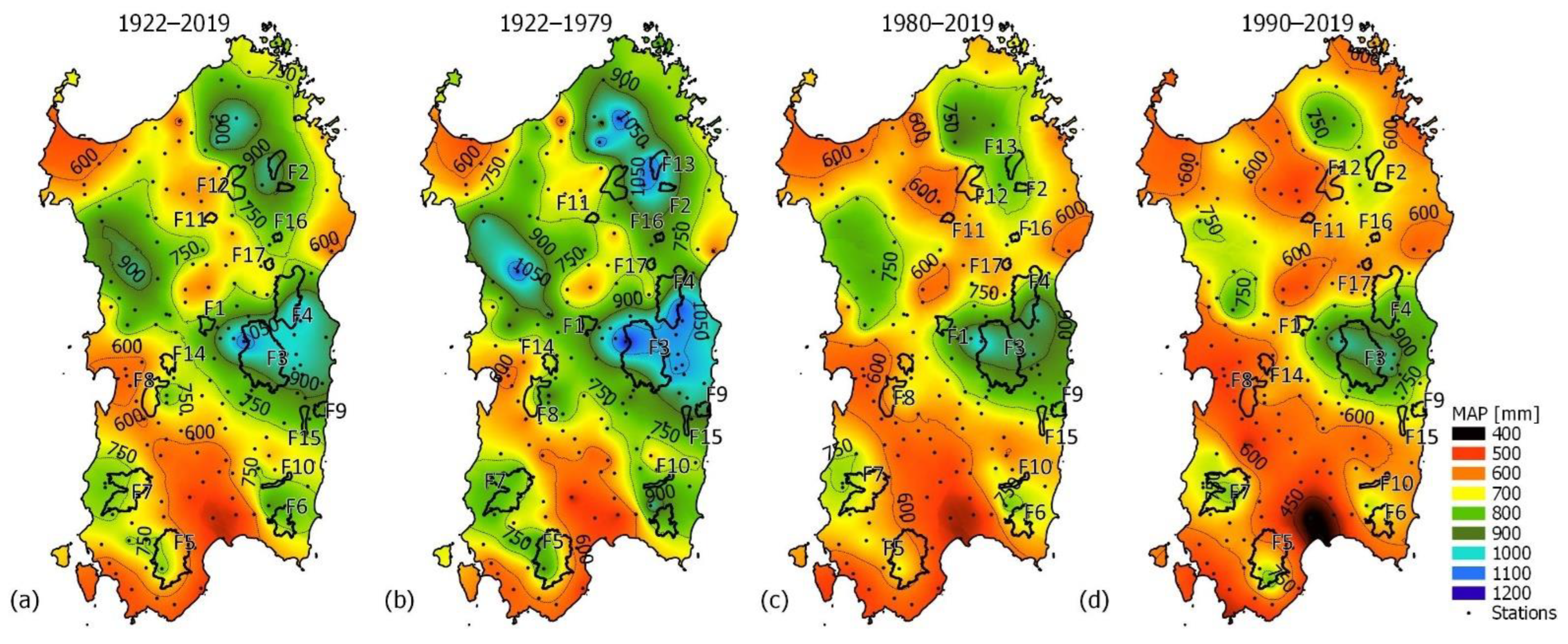
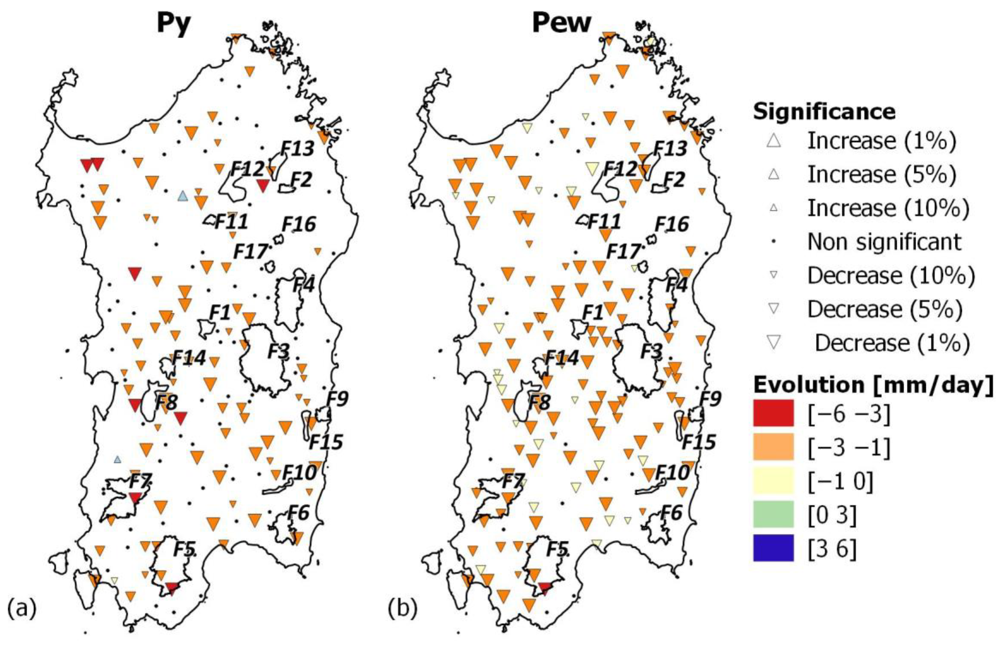
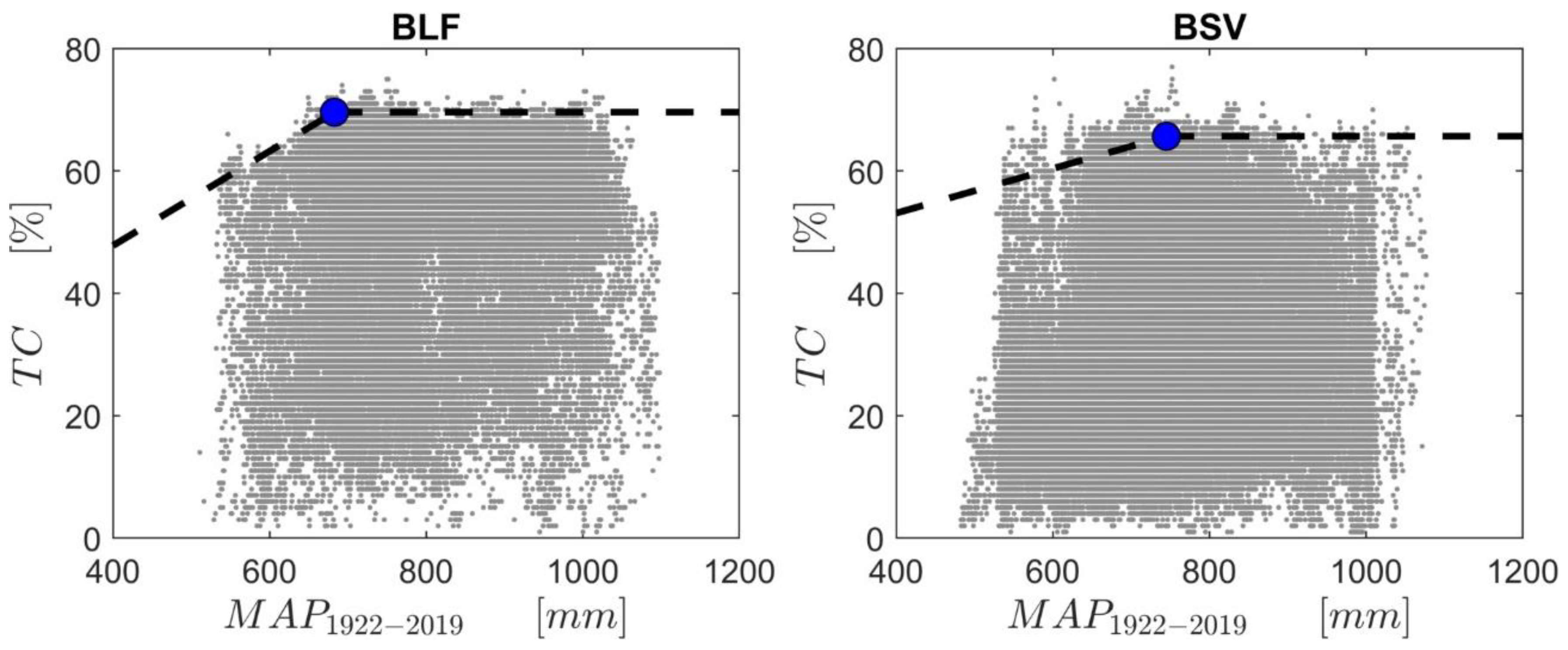
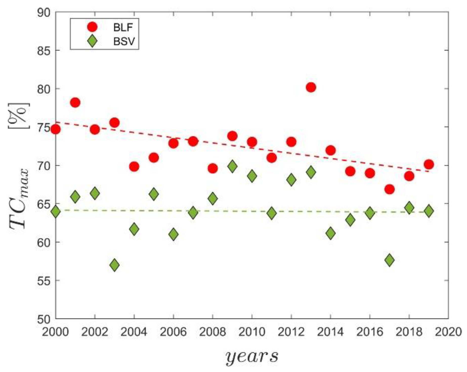
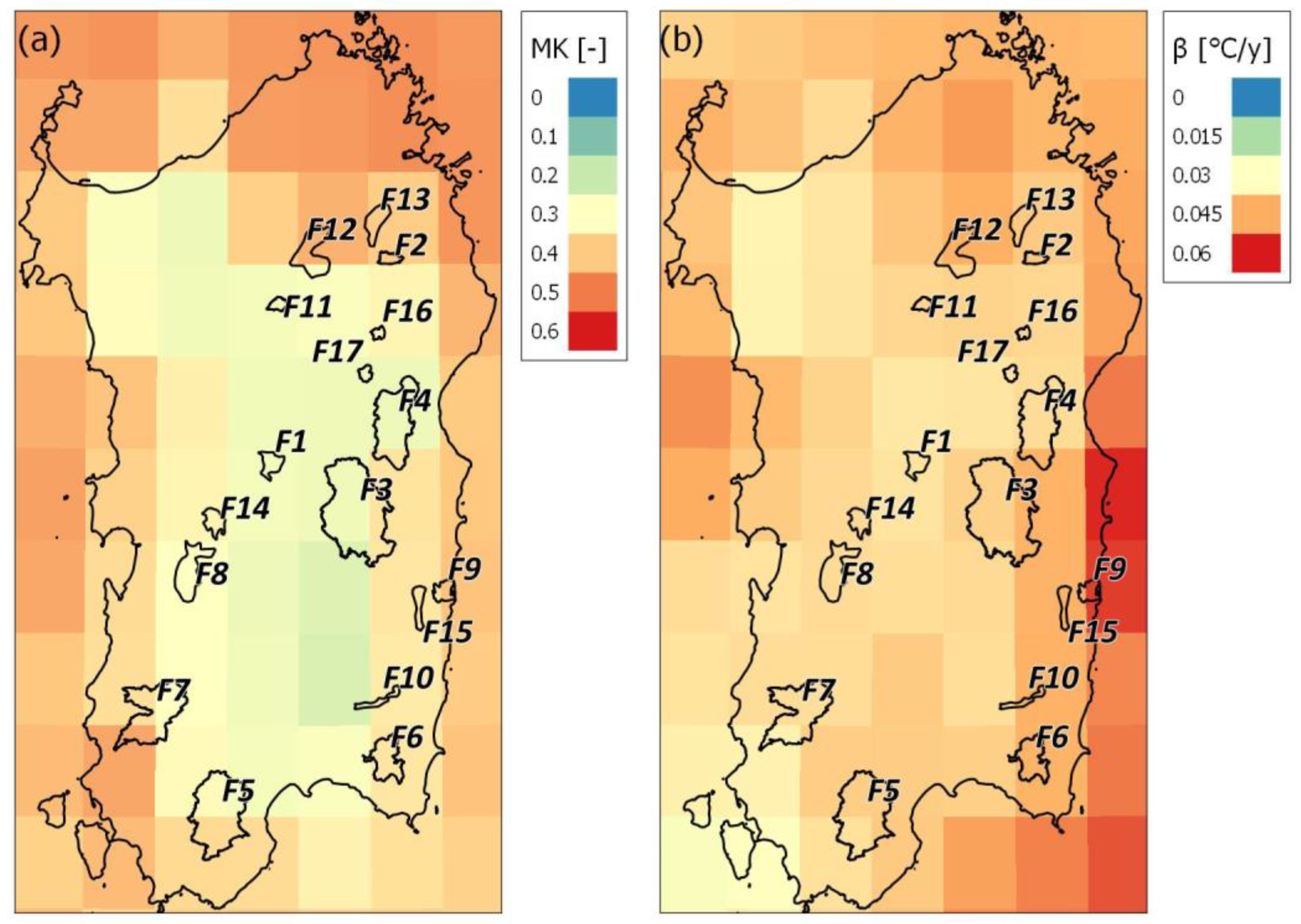
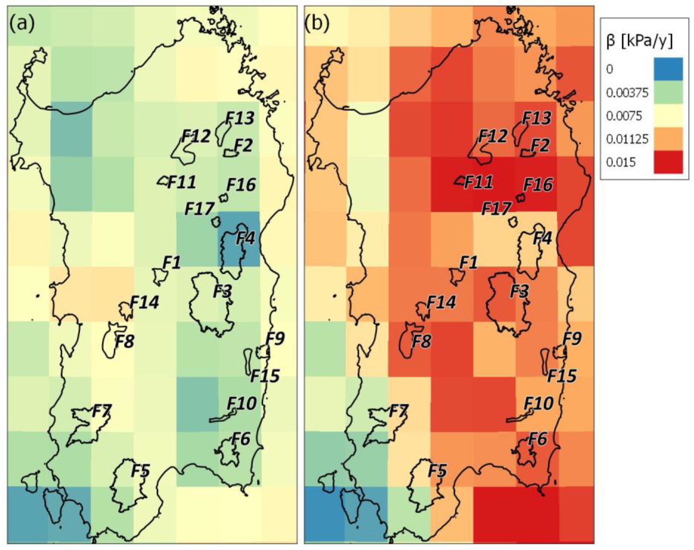
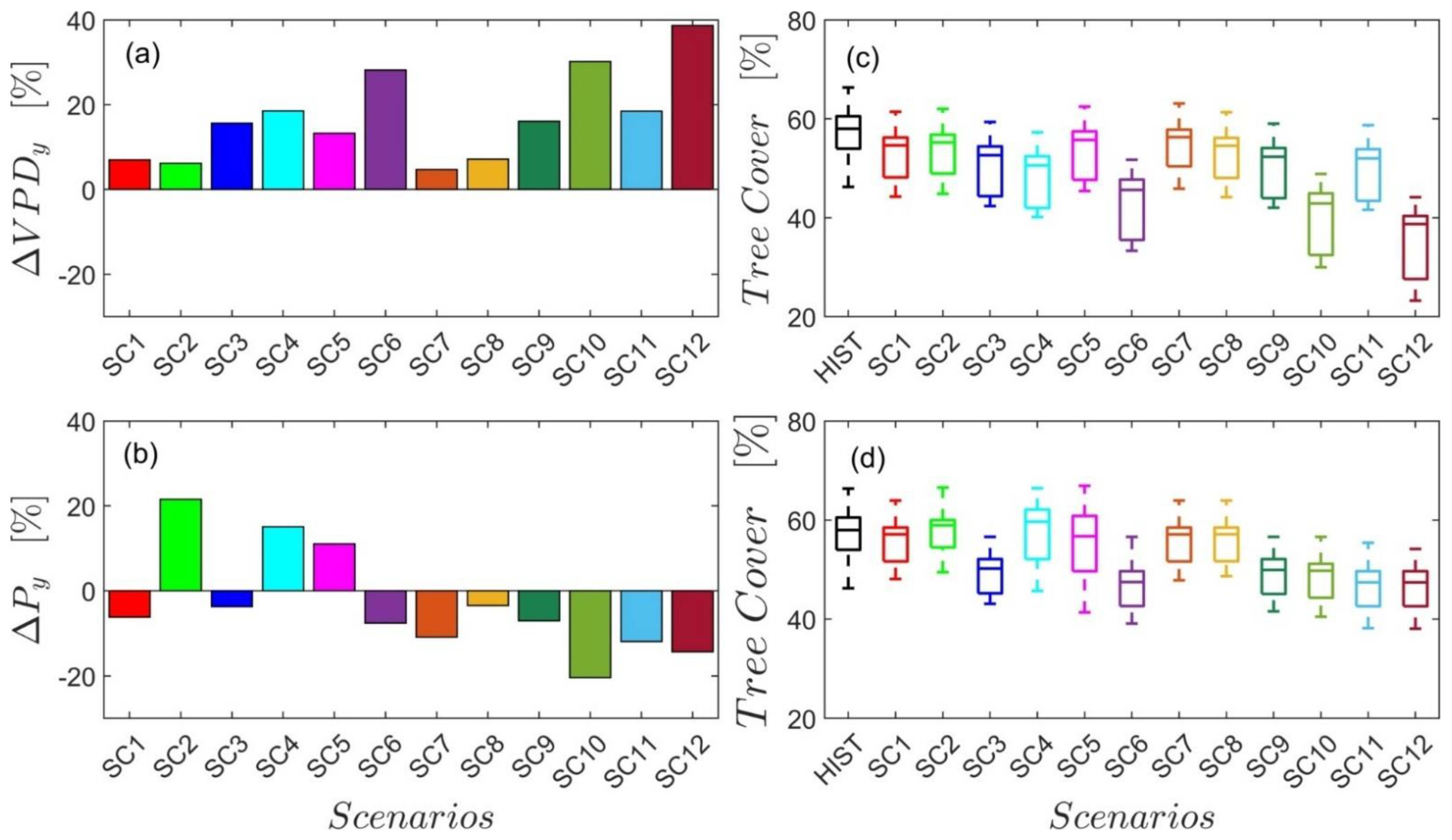
Table 1.
Corine Land Cover classification and description of the land cover analyzed by this study.
| CLC Class ID | Description |
|---|---|
| 3.1.1. | Broad-leaved forest (BLF) Vegetation formation composed principally of trees, including shrub and bush understory, where broad-leaved species predominate. This class is applicable for mature forests of natural or anthropogenic origin. In Sardinia, it mainly includes evergreen broad-leaved woodlands composed of sclerophyllous trees (mainly Quercus Ilex, Quercus suber, Quercus Rotondifolia). Broad-leaved area must cover at least 75% of the forest tree component. |
| 3.1.2. | Coniferous forest (CF) Woodlands consisting mainly of trees, but also of bushes and shrubs, in which coniferous forest species dominate. This class is applicable for mature coniferous (needle-leaved) forests of natural or anthropogenic origin pure or mixed stands of fir (Abies), pine (Pinus), spruce (Picea), cedar (Cedrus), cypress (Cupressus), juniper (Juniperus), yew (Taxus), and species, among others. The coniferous surface must constitute at least 75% of the forest tree component. |
| 3.2.3. | Bushy sclerophyllous vegetation (BSV) Bushy sclerophyllous vegetation in a climax stage of development, including maquis, matorral, garrigue, and thermo-Mediterranean brushes, characterized by shrubs of sclerophyllous character (Quercus, P. latifolia, Pistacia lentiscus, Arbutus unedo, Mirtus, Juniperus, Cistus, Lavandula, Rosmarinus, Euphorbia, Genista, Erica, Laurus, etc., species), with hard leaves and short internodes, usually evergreen. |
Table 2.
Properties of the 17 Sardinian forests indicated in Figure 1: code; name; surface; mean altitude; and percentage of the surface covered by broad-leaved vegetation (BLF), bushy sclerophyllous vegetation (BSV), coniferous forest (CF), and other vegetation.
Table 2.
Properties of the 17 Sardinian forests indicated in Figure 1: code; name; surface; mean altitude; and percentage of the surface covered by broad-leaved vegetation (BLF), bushy sclerophyllous vegetation (BSV), coniferous forest (CF), and other vegetation.
| Code | Name | Surface | Mean Altitude | Surface Covered by BLF | Surface Covered by BSV | Surface Covered by CF | Surface Covered by Other Vegetation |
|---|---|---|---|---|---|---|---|
| (-) | (km2) | (m asl) | (%) | (%) | (%) | (%) | |
| F1 | Barigadu | 36.23 | 639.8 | 43% | 35% | 5% | 17% |
| F2 | Sos Littos—Sas Tumbas (Bitti) | 19.27 | 378.2 | 73% | 7% | 2% | 18% |
| F3 | Monti del Gennargentu | 447.53 | 1047.3 | 24% | 8% | 3% | 65% |
| F4 | Supramonte di Oliena, Orgosolo e Urzulei—Su Sercone | 235.08 | 765.9 | 26% | 17% | 2% | 54% |
| F5 | Foresta di Monte Arcosu | 303.8 | 449.6 | 52% | 24% | - | 24% |
| F6 | Monte dei Sette Fratelli e Sarrabus | 92.98 | 531.5 | 72% | 11% | - | 17% |
| F7 | Monte Linas—Marganai | 236.46 | 551.8 | 26% | 28% | - | 46% |
| F8 | Monte Arci | 101.82 | 414 | 32% | 35% | 5% | 28% |
| F9 | Monte Ferru | 32.05 | 336.7 | 28% | 36% | 0% | 37% |
| F10 | Villasalto | 22.79 | 490.5 | 2% | 73% | 15% | 10% |
| F11 | Fiorentini | 15.88 | 796.4 | 85% | - | - | 15% |
| F12 | Monte Lerno | 99.26 | 612.9 | 22% | 26% | 25% | 27% |
| F13 | Sorilis | 49.92 | 548.2 | - | 50% | 12% | 38% |
| F14 | Siamanna | 37.93 | 343 | 0% | 56% | 13% | 31% |
| F15 | Tacchixeddu | 29.07 | 461.5 | 19% | 55% | 6% | 20% |
| F16 | Su Sartu | 11.03 | 555.5 | - | 41% | - | 59% |
| F17 | Nuoro | 14.2 | 630.5 | 54% | 16% | - | 30% |
Table 3.
The mean Mann-Kendall τ and the Theil-Sen slope β of the tree canopy coverage (TC), non-tree vegetation (NTV), and non-vegetated (bare) coverage (BS) for all the broad-leaved forests (BLFs) and bushy sclerophyllous vegetation (BSV) observed pixels falling within each of the 17 sites analyzed.
| Code | τTCBLF | τTCBSV | τNTVBLF | τNTVBSV | τBSBLF | τBSBSV | βTCBLF | βTCBSV | βNTVBLF | βNTVBSV | βBSBLF | βBSBSV |
|---|---|---|---|---|---|---|---|---|---|---|---|---|
| (-) | (-) | (-) | (-) | (-) | (-) | (%TC/y) | (%TC/y) | (%NTC/y) | (%NTC/y) | (%BS/y) | (%BS/y) | |
| F1 | −0.15 | 0.06 | 0.08 | −0.07 | 0.10 | 0.01 | −0.16 | 0.14 | 0.07 | −0.16 | 0.08 | 0.01 |
| F2 | −0.12 | 0.04 | 0.10 | −0.03 | 0.02 | −0.07 | −0.15 | 0.09 | 0.14 | −0.07 | 0.07 | −0.02 |
| F3 | 0.03 | −0.11 | 0.02 | 0.05 | −0.12 | −0.24 | 0.12 | −0.24 | 0.05 | 0.35 | −0.14 | −0.20 |
| F4 | 0.00 | 0.06 | 0.06 | −0.05 | −0.14 | −0.02 | 0.05 | 0.12 | 0.11 | −0.12 | −0.14 | 0.01 |
| F5 | −0.30 | 0.09 | 0.18 | 0.00 | 0.00 | −0.16 | −0.30 | 0.20 | 0.30 | −0.03 | 0.00 | −0.09 |
| F6 | −0.12 | 0.11 | 0.03 | −0.13 | 0.11 | 0.11 | −0.09 | 0.19 | 0.02 | −0.29 | 0.10 | 0.06 |
| F7 | −0.10 | 0.22 | 0.03 | −0.15 | 0.11 | −0.19 | −0.11 | 0.35 | 0.01 | −0.27 | 0.09 | −0.09 |
| F8 | −0.19 | 0.14 | 0.06 | −0.15 | 0.25 | 0.05 | −0.21 | 0.20 | 0.05 | −0.32 | 0.34 | 0.13 |
| F9 | −0.14 | 0.27 | 0.02 | −0.19 | 0.17 | −0.07 | −0.15 | 0.50 | 0.01 | −0.41 | 0.10 | −0.01 |
| F10 | −0.21 | −0.03 | - | −0.01 | 0.08 | 0.04 | −0.19 | −0.06 | NaN | −0.01 | 0.02 | 0.07 |
| F11 | −0.09 | 0.09 | 0.05 | 0.02 | −0.03 | −0.15 | −0.09 | 0.17 | 0.09 | −0.01 | 0.01 | −0.15 |
| F12 | −0.09 | 0.15 | 0.03 | 0.12 | 0.06 | −0.30 | −0.10 | 0.22 | 0.04 | 0.17 | 0.04 | −0.35 |
| F13 | - | 0.01 | - | −0.01 | - | 0.01 | - | 0.01 | - | −0.04 | - | 0.01 |
| F14 | - | 0.07 | - | −0.10 | - | 0.08 | - | 0.13 | - | −0.20 | - | 0.05 |
| F15 | −0.29 | 0.08 | 0.19 | −0.07 | 0.10 | −0.03 | −0.22 | 0.14 | 0.22 | −0.16 | 0.06 | 0.01 |
| F16 | - | 0.01 | - | −0.04 | - | 0.10 | - | 0.07 | - | −0.13 | - | 0.07 |
| F17 | −0.07 | 0.04 | 0.03 | −0.07 | 0.07 | 0.02 | −0.05 | 0.11 | 0.02 | −0.14 | 0.04 | 0.04 |
Table 4.
Pearson correlation coefficients (ρ), and relative p-value between the Theil-Sen slope estimators of the percentage of tree cover and bare soil in broad–leaved (βTCBLF and βBSBLF) and in bushy sclerophyllous vegetation (βTCBSV and βBSBSV) with some of the main climate variables.
Table 4.
Pearson correlation coefficients (ρ), and relative p-value between the Theil-Sen slope estimators of the percentage of tree cover and bare soil in broad–leaved (βTCBLF and βBSBLF) and in bushy sclerophyllous vegetation (βTCBSV and βBSBSV) with some of the main climate variables.
| βTCBLF | βTCBSV | βBSBLF | βBSBSV | |||||
|---|---|---|---|---|---|---|---|---|
| ρ | p-val | ρ | p-val | ρ | p-val | ρ | p-val | |
| MAP1990–2019 | 0.71 | 0.004 | 0.13 | 0.46 | −0.68 | 0.01 | −0.44 | 0.07 |
| βTes | −0.22 | 0.45 | −0.13 | 0.61 | 0.02 | 0.24 | 0.18 | 0.49 |
| βTew | −0.22 | 0.45 | −0.09 | 0.73 | 0.05 | 0.70 | 0.14 | 0.60 |
| βTsf | −0.27 | 0.35 | −0.01 | 0.98 | −0.03 | 0.35 | 0.13 | 0.62 |
| βTss | 0.04 | 0.91 | 0.16 | 0.53 | 0.00 | 0.89 | −0.23 | 0.38 |
| βTy | −0.33 | 0.25 | −0.07 | 0.78 | −0.09 | 0.25 | 0.35 | 0.17 |
| βVPDes | −0.12 | 0.68 | −0.42 | 0.09 | 0.16 | 0.52 | 0.27 | 0.30 |
| βVPDew | −0.31 | 0.28 | 0.01 | 0.97 | −0.13 | 0.39 | 0.26 | 0.32 |
| βVPDsf | −0.32 | 0.26 | −0.34 | 0.18 | 0.04 | 0.08 | 0.32 | 0.21 |
| βVPDss | −0.28 | 0.33 | −0.39 | 0.12 | 0.00 | 0.10 | 0.46 | 0.06 |
| βVPDy | −0.61 | 0.02 | −0.34 | 0.18 | −0.62 | 0.02 | 0.44 | 0.08 |
| Future Scenario | Coupled Model Intercomparison Project Phase | Representative Concentration Pathways | Shared Socioeconomic Pathways | Period |
|---|---|---|---|---|
| SC1 | CMIP5 | RCP 45 | 2020–2030 | |
| SC2 | CMIP5 | RCP 85 | - | 2020–2030 |
| SC3 | CMIP5 | RCP 45 | - | 2055–2075 |
| SC4 | CMIP5 | RCP 85 | - | 2055–2075 |
| SC5 | CMIP5 | RCP 45 | - | 2081–2090 |
| SC6 | CMIP5 | RCP 85 | - | 2081–2090 |
| SC7 | CMIP6 | - | SSP 245 | 2020–2030 |
| SC8 | CMIP6 | - | SSP 585 | 2020–2030 |
| SC9 | CMIP6 | - | SSP 245 | 2055–2075 |
| SC10 | CMIP6 | - | SSP 585 | 2055–2075 |
| SC11 | CMIP6 | - | SSP 245 | 2081–2090 |
| SC12 | CMIP6 | SSP 585 | 2081–2090 |
Publisher’s Note: MDPI stays neutral with regard to jurisdictional claims in published maps and institutional affiliations. |
© 2022 by the authors. Licensee MDPI, Basel, Switzerland. This article is an open access article distributed under the terms and conditions of the Creative Commons Attribution (CC BY) license (https://creativecommons.org/licenses/by/4.0/).
Share and Cite
MDPI and ACS Style
Cipolla, S.S.; Montaldo, N. On the Impacts of Historical and Future Climate Changes to the Sustainability of the Main Sardinian Forests. Remote Sens. 2022, 14, 4893. https://0-doi-org.brum.beds.ac.uk/10.3390/rs14194893
AMA Style
Cipolla SS, Montaldo N. On the Impacts of Historical and Future Climate Changes to the Sustainability of the Main Sardinian Forests. Remote Sensing. 2022; 14(19):4893. https://0-doi-org.brum.beds.ac.uk/10.3390/rs14194893
Chicago/Turabian StyleCipolla, Sara Simona, and Nicola Montaldo. 2022. "On the Impacts of Historical and Future Climate Changes to the Sustainability of the Main Sardinian Forests" Remote Sensing 14, no. 19: 4893. https://0-doi-org.brum.beds.ac.uk/10.3390/rs14194893
Note that from the first issue of 2016, this journal uses article numbers instead of page numbers. See further details here.