A High Spatiotemporal Enhancement Method of Forest Vegetation Leaf Area Index Based on Landsat8 OLI and GF-1 WFV Data

Abstract

The leaf area index (LAI) is a crucial parameter for analyzing terrestrial ecosystem carbon cycles and global climate change. Obtaining high spatiotemporal resolution forest stand vegetation LAI products over large areas is essential for an accurate understanding of forest ecosystems. This study takes the northwestern part of the Inner Mongolia Autonomous Region (the northern section of the Greater Khingan Mountains) in northern China as the research area. It also generates the LAI time series product of the 8-day and 30 m forest stand vegetation growth period from 2013 to 2017 (from the 121st to the 305th day of each year). The Simulated Annealing-Back Propagation Neural Network (SA-BPNN) model was used to estimate LAI from Landsat8 OLI, and the multi-period GaoFen-1 WideField-View satellite images (GF-1 WFV) and the spatiotemporal adaptive reflectance fusion mode (STARFM) was used to predict high spatiotemporal resolution LAI by combining inversion LAI and Global LAnd Surface Satellite-derived vegetation LAI (GLASS LAI) products. The results showed the following: (1) The SA-BPNN estimation model has relatively high accuracy, with R² = 0.75 and RMSE = 0.38 for the 2013 LAI estimation model, and R² = 0.74 and RMSE = 0.17 for the 2016 LAI estimation model. (2) The fused 30 m LAI product has a good correlation with the LAI verification of the measured sample site (R² = 0.8775) and a high similarity with the GLASS LAI product. (3) The fused 30 m LAI product has a high similarity with the GLASS LAI product, and compared with the GLASS LAI interannual trend line, it accords with the growth trend of plants in the seasons. This study provides a theoretical and technical reference for forest stand vegetation growth period LAI spatiotemporal fusion research based on high-score data, and has an important role in exploring vegetation primary productivity and carbon cycle changes in the future.

1. Introduction

The leaf area index (LAI) is defined as the area formed by vegetation growth and photosynthesis, accounting for half of the total leaf area of surface plants per unit area, which controls physiological and biological processes, such as vegetation growth, respiration, and transpiration [1,2,3]. Therefore, the LAI is very important in the study of how biological and geochemical cycle models and terrestrial ecosystem carbon–water cycle models should be constructed [4,5,6]. Thus, obtaining high-precision and high-quality LAI products will help people improve their knowledge and understanding of the geochemical carbon–water cycle of land and ecosystems, and their environmental responses to global climate change.

Obtaining large-scale forest LAIs with the help of remote sensing technology has gradually become the main method and means for the study of vegetation ecological environments. Currently, LAI estimation can be broadly categorized into three primary approaches: physical models, empirical models, and hybrid models [7,8]. The majority of LAI estimation methods rely on a single remote sensing dataset, which can constrain the ability to explore the temporal and spatial dynamics of LAI fully. Neural networks have great advantages when used to deal with linear and complex nonlinear problems [9,10]. Many scholars have introduced artificial neural networks (ANN) into the model research of LAI inversion [11,12], among which the backpropagation neural network (BPNN) has a multi-layer nonlinear network structure and strong robustness of the model, and is widely used [13,14]. Yang Min et al. used Landsat8 OLI and measured data to simulate the BPNN model, and its inversion accuracy is higher than that of the traditional regression model [15]. Zhu, D.E. et al. demonstrated that the BPNN method, utilizing MODIS reflective time-series data, is capable of accurately estimating LAI for the Lei bamboo forest [16]. However, some scholars indicated that the BPNN model has shortcomings, such as its slow network model training and the fact that it easily falls into a local minimum, which affects the training accuracy [17]. The simulated annealing (SA) algorithm is a relatively novel random search algorithm, and the original idea came from the annealing process of solid object space. Hong Min Zhou et al. found that the SA algorithm is a heuristic algorithm for complex nonlinear optimization problems, which can be used to extend the local range search algorithm to find the optimal solution in a larger space [18]. In summary, the Simulated Annealing-Back Propagation Neural Network model (SA-BPNN) uses a simulated annealing algorithm to avoid local minimum, and improve convergence speed and accuracy. It can adaptively adjust the learning rate and inertia factor, and reduce the complexity of parameter setting. It also has stronger generalization ability and robustness. Additionally, SA-BPNN is suitable for smaller-scale data sets; using SA-BPNN can effectively reduce the consumption of computing resources while avoiding the risk of over-fitting. In this study, the global search capability of the SA algorithm was utilized to optimize the initial weight value and threshold of the BPNN. The error backpropagation method was then used to find the optimal solution of the model.

Most current LAI products cannot simultaneously satisfy the requirements of high temporal resolution and high spatial resolution at the same time. In order to solve this technical problem, scholars proposed the concept of “image fusion” [19,20,21]. Its principle is to introduce the concept of adjacent pixels based on the spatiotemporal fusion model of the image reconstruction type and use interpolation operations to generate fusion pixels according to the careful consideration of pixel spectral similarity, temporal distance, and spatial similarity [22,23,24]. Among them, the most representative is the spatiotemporal adaptive reflectance fusion model (STARFM) [25] proposed by Gao et al. In essence, the model is used to determine the pixels similar to the spectral characteristics of the central pixel through unsupervised classification and threshold segmentation in the defined search window, and sample filtering is performed on these pixels to obtain pixels that can provide sufficient reflectance information. The effective pixel reflectance is integrated by combining weighted methods to calculate the central pixel, which is used to predict the value of the reflectance at a certain position at a certain time of day. At present, when scholars choose to fuse images, most of them fuse MODIS and Landsat images, basically forming a standard processing flow. Caroline M. Gevaert et al. successfully applied the STARFM model to combine MODIS and Landsat8 reflectance data, producing high-temporal-resolution and high-spatial-resolution surface reflectance data that demonstrated a strong correlation with verified and real image data [26]. Yuan Zhoumiqi et al. evaluated the suitability of the spatiotemporal remote sensing data fusion algorithm (DDSTDFA) for large-scale high-spatiotemporal-resolution image data fusion using Landsat8 OLI and three high-temporal-resolution datasets, confirming its potential for monitoring dynamic changes in large-scale forest vegetation [27]. With the development of high-scoring Chinese satellites, some scholars have also tried to use high-scoring Chinese data for fusion. Tao G et al. and Wang S et al. explored the application characteristics of GF-1 WFV in image fusion by fusing MODIS and GF-1 WFV or Sentinel-2 and GF-1 WFV data surface reflectance [28,29].

This study developed a method to generate a time series of forest stand vegetation growth LAI over the northwestern region of Inner Mongolia, China. The method utilized data from Landsat8 OLI, GF-1 WFV, and GLASS LAI to obtain 8-day and 30 m resolution LAI inversion during the growth period (121st to 305th day of each year). This study utilized the SA-BPNN model to derive LAI maps from Landsat8 OLI and GF-1 WFV images. The resultant fine-resolution LAI maps were further combined with the temporally continuous GLASS LAI product using the STARFM algorithm, which enabled the incorporation of spatiotemporal characteristics from multiple data sources. The accuracy and consistency of the LAI time series data were evaluated by comparing and validating the results with ground measurements, thus assessing the spatiotemporal performance of the LAI data. The research results provide theoretical and technical references for LAI spatiotemporal fusion research based on high-resolution data and then provide long-term LAI data with high spatiotemporal resolutions for the study of carbon cycle changes.

2. Materials and Methods

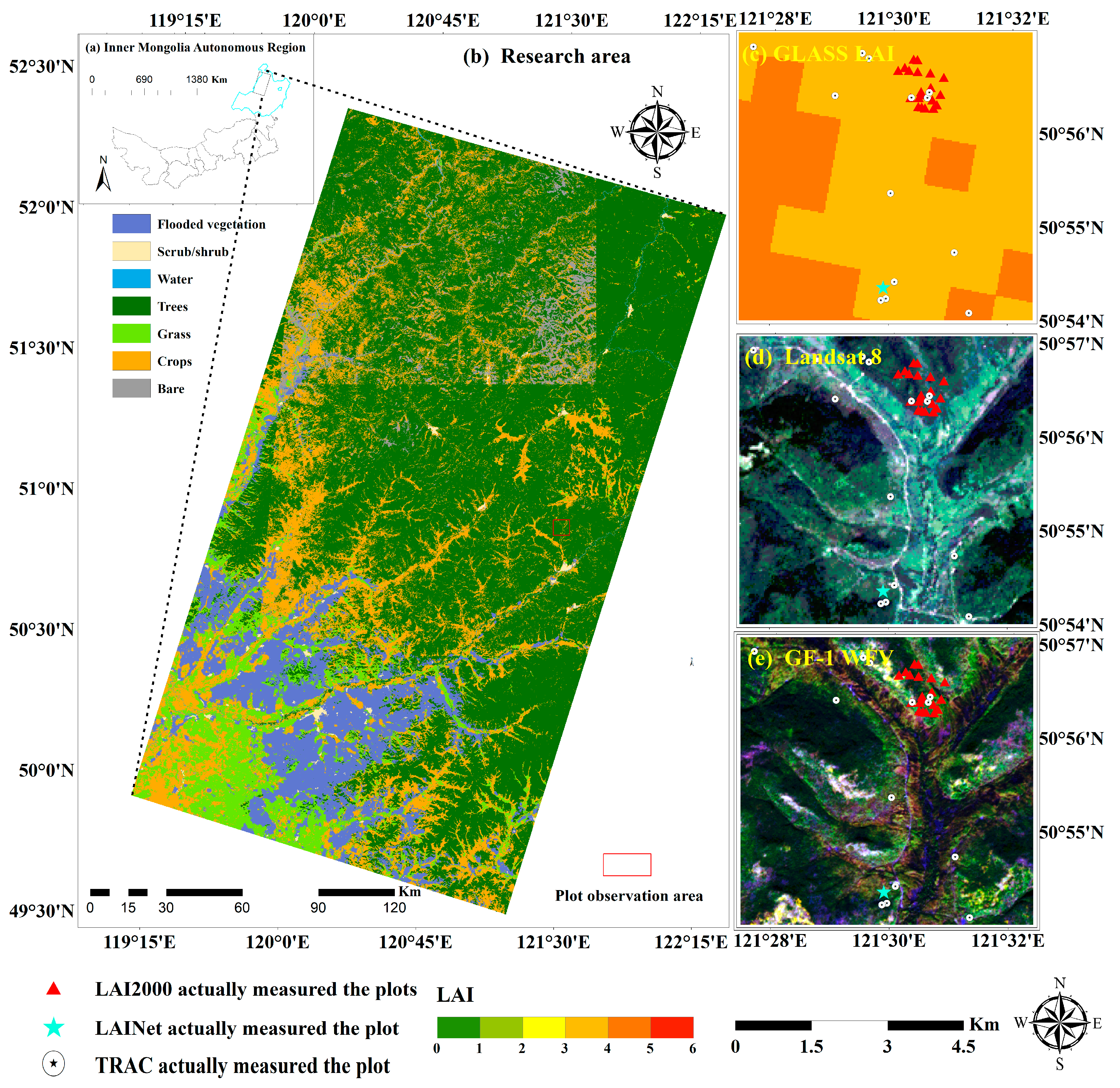
2.1. Study Area

The study area was located in the northwestern part of Hulunbeir City, Inner Mongolia Autonomous Region of China, and the western part of the Greater Khingan Mountains Key State Forest Area (119°9′–122°26′E, 49°33′–52°24′N, Figure 1), with a total area of about 45,000 km². The average altitude of this area is 1000 m. It is a middle-high-latitude area of Eurasia, with long winters and short summers. The annual precipitation reaches 10~280 mm, mainly concentrated in July~September in summer. The forest is mainly composed of Pinus sylvestris var. mongholica, Larix spp., and Betula platyphylla. The LAI-2000 observation points (triangles) were located in the 20 plots (Standard plot 30 m × 30 m), and the LAINet observation points (five-pointed star) were located in the No. 4 Ecological Station of the Genhe Experimental Area. The sample plot used in this study is a standardized plot with dimensions of 30 m by 30 m. This aspect ratio was chosen to ensure consistency in the size and shape of the plot across all measurements and to facilitate accurate comparisons between different data sets.

2.2. Datasets and Processing

2.2.1. Satellite Data

The Global Land Surface Satellite of LAI (GLASS LAI) is a high-quality remote sensing data product with independent intellectual property rights in China. The GLASS LAI is a relational model from preprocessed data MOD09A1 to LAI value based on the artificial neural network method, which is used to produce global land surface leaf area index products. During production, it was processed by removing clouds and snow, filling missing values, and filtering [30]. As a result, the GLASS LAI products offer global land surface coverage with a spatial resolution of 1 km and 0.05° and a temporal resolution of 8 days. Compared to other products such as MODIS and CYCLOPES, GLASS LAI products offer a higher spatial resolution, greater precision, global coverage, multi-temporal data, and higher update frequency. These advantages enable GLASS LAI products to provide more comprehensive and accurate vegetation coverage information, making it a powerful tool for research and applications in related fields. In addition, it is the most complete and time-continuous product in space, providing robust data support for various applications.

In practical applications, reductions may increase errors or have other advantages. It was downloaded from the National Center for Earth System Science Data (http://www.geodata.cn/thematicView/GLASS.html (accessed on 1 May 2022)); Landsat8 OLI can be downloaded from the USGS website (https://earthexplorer.usgs.gov/ (accessed on 1 May 2022)). In this study, GF-1 WFV was used to obtain data for other years; GF-1 WFV data was obtained from the China Resources Satellite Application Center (http://www.cresda.com/CN/ (accessed on 1 May 2022)). GF-1 WFV data image spatial resolution is 16 m, and the temporal resolution is 4 days, including four blue, green, red, and near-infrared bands. The image acquisition time is 27 September 2013, 22 August 2016, and 20 September 2017. The Finer Resolution Observation and Monitoring of Global Land Cover (FROM-GLC-seg) product has been produced with high overall accuracy (the overall accuracy is 72.76% [31]) from both Landsat TM and ETM+ data. It is a land product with global coverage, obtained by being downloaded from the Tsinghua University website (http://0-data-ess-tsinghua-edu-cn.brum.beds.ac.uk/index.html (accessed on 1 May 2022)). Details regarding the data are shown in

Table 1. Information of each remote sensing and GLASS LAI dataset.

Sensor	Band	Spectral Range (nm)	Acquisition Time (DOY)	Spatial Resolution	Revisit Period
Landsat8 OLI	1–AEROSOL	435–451	2014 (151) 2015 (186)	30 m	16-days
	2–Blue	452–512
	3–Green	533–590
	4–Red	636–673
	5–NIR	851–879
	6–SWIR1	1560–1651
	7–SWIR2	2107–2294
GF-1 WFV	1–Blue	450–520	2013 (270) 2016 (235) 2017 (263)	16 m	4-days
	2–Green	520–590
	3–Red	630–690
	4–NIR	770–890
GLASS LAI	/	/	2013–2017 (121–128, 129–136, 137–144, 145–152, 153–160, 161–168, 169–176, 177–184, 185–192, 193–200, 201–208, 209–216, 217–224, 225–232, 233–240, 241–248, 249–256, 257–264, 265–272, 273–280, 281–288, 289–296, 297–305)	1 km	8-days

Acquisition time: Day of year is abbreviated as DOY.

.

2.2.2. Field Measurements Using LAI Datasets

The verification data set mainly includes two main parts: (1) the LAI-2000 observation data; (2) the LAINet, TRAC, and LAI-2200 observation system data. Data details are shown in

Table 2. Details of Field measurements LAI data.

LAI	Collection Time (DOY)	Number of Samples
LAI 2000	2013 (221, 223, 226, 227, 247)	53
	2016 (147, 157, 169, 185, 199, 215, 230, 248, 260, 266)	140
LAINet	2013 (221, 223, 226, 227, 247)	50
TRAC	2013 (224, 232, 248)	13
LAI 2200	2013 (222, 225, 228)	9

Collection time: Day of year is abbreviated as DOY.

.

Regarding the LAI-2000 observation data set of 20 plots in the experimental area of Genhe City [32], two LAI-2000s were used for synchronous observation. One instrument was erected and fixed in the open space to measure the skylight, and the other instrument was used to measure light changes under the forest canopy. The FV2000 program was used to export the data of the two instruments and combine them to calculate the measurement results of various places.

The LAINet observation system datasets were built from the No. 4 (L3) plot of the Ecological Station of the Genhe Experimental Area. The LAINet data were measured using the wireless sensor network LAI observer made by Beijing Normal University. The observation system was divided into three parts: the observation upper node, the lower observation node, and the convergence node. The source of the data was the LAINet observation data set of the No. 4 (L3, 50°54.318′N, 121°29.9325′E) plot of the Genhe Experimental Area Ecological Station (2013) by Qu Yonghua. Daily LAI data were recorded (except for on the 233rd to 240th day due to device failure). Since the observation time was short, we used TRAC LAI and LAI-2200 LAI as DOY validation data for a single day. Data were collected using the TRAC (Tracing Radiation and Architecture of Canopies) instrument, and the mean value of each of the 13 standard plots was taken as one set of data. Data were also collected using the LAI-2200 instrument, and the mean value of each of the 9 standard plots was taken as one set of data.

2.2.3. Remote Sensing Image Dataset Preprocessing

The remote sensing image preprocessing method used in this experiment mainly included Rational Polynomial Coefficient (RPC) orthorectification, radiometric calibration, atmospheric correction, and resampling, among which GLASS LAI was also used to perform reprojection, splicing, and cropping.

Radiation calibration was carried out in the ENVI module Radiometric calibration. Gain and offset values needed to be added to the image before calibration. Landsat8 OLI and GF-1 images were set according to the relevant parameters of the downloaded image file; this research uses the RPC module [33,34] in orthorectification, the RPC parameters included with GF-1 WFV data are used for correction, the DEM data required for correction is from ASTER satellite’s 30 m spatial resolution GDEM product (https://www.gscloud.cn/search?kw=GF-1 (accessed on 1 May 2022)), eliminating the geometric distortion caused by the influence of the mountain, and the deformation caused by the camera orientation; the atmospheric correction was performed on Landsat8 OLI and GF-1 WFV through the FLASSH atmospheric correction module [35,36]. As a result, the influence of external factors such as atmosphere and light on the image was eliminated, and a more accurate surface reflectance was obtained.

In this study, the spatial resolution of GF-1 WFV is 16 m. To ensure that the image resolution is the same during the fusion process, we resampled the GF-1 WFV image data to match the spatial resolution of Landsat 8 OLI, which is 30 m. Additionally, the spatial resolution of GLASS LAI is 1 km. Firstly, we used the MODIS Reprojection Tool (MRT) [37,38] to reproject the data to the UTM-WGS84 coordinate system. Then, we performed data mosaicking. Finally, we resampled the image to 30 m × 30 m in ENVI and cropped it to the range of the study area.

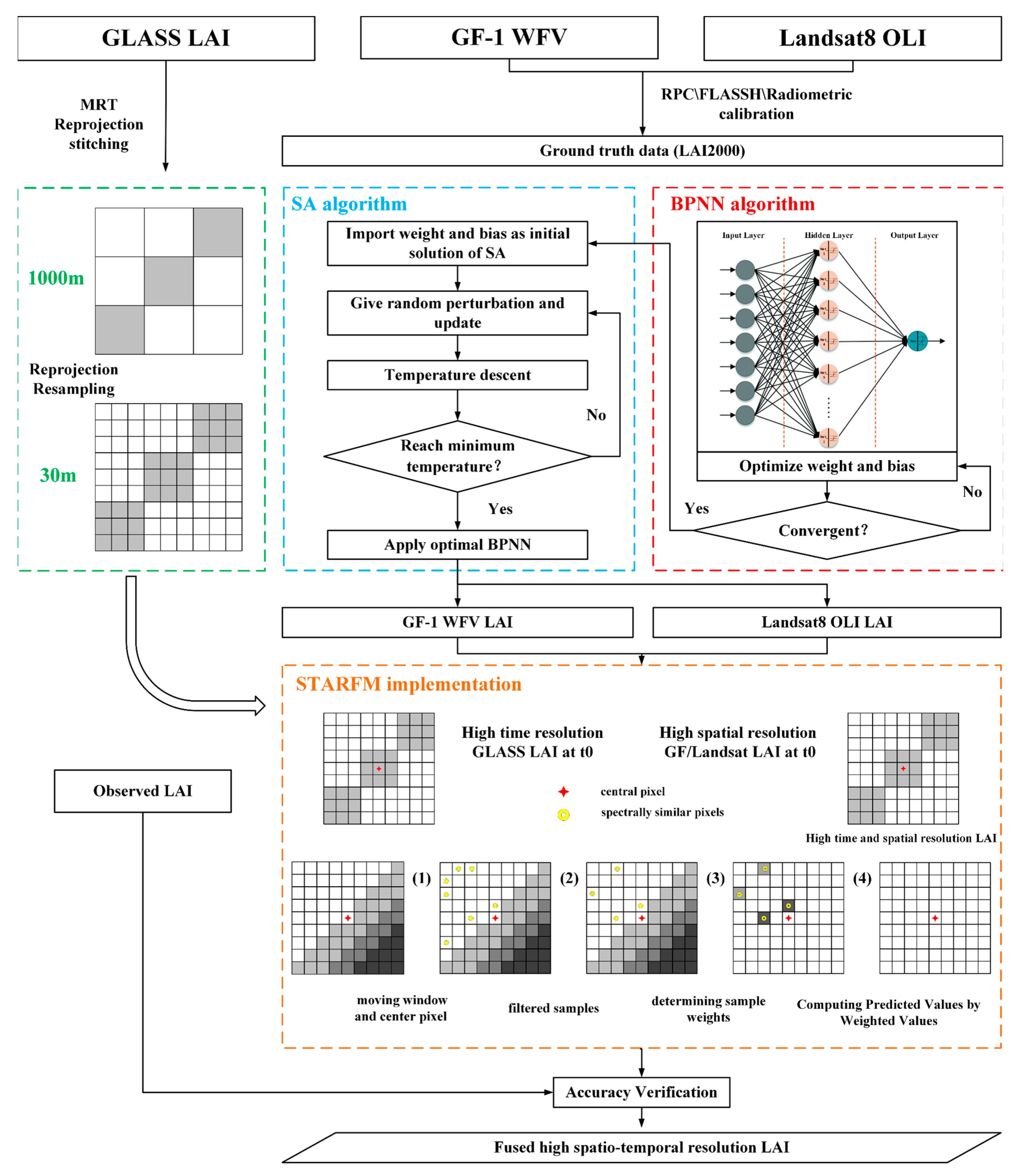
2.3. LAI Data Fusion Based on the STARFM Model

In this study, an SA-BPNN model was established to estimate the LAI using image datasets of the 4-band reflectance of GF-1 WFV or the 7-band reflectance of Landsat8 OLI, and actual measurements obtained from LAI-2000. Then, the estimated LAI was then fused with GLASS LAI. Finally, the fused LAI was compared to the actual measurement data from the LAINet, TRAC LAI, and LAI-2200 datasets with the same resolution for inspection. The main steps of the research included:

(1)

The acquisition and preprocessing: acquisition and preprocessing of remote sensing image data and verification data;

(2)

GF-1 WFV and Landsat8 OLI images, along with ground-measured LAI-2000 data, were preprocessed and used to train the SA-BPNN model. The model was then utilized to estimate LAI for GF-1 WFV (2013, 2016, and 2017) and Landsat8 OLI (2014 and 2015) images;

(3)

The estimated GF-1 WFV LAI and Landsat8 OLI LAI were fused with GLASS LAI (2013~2017) using the STARFM model to obtain an LAI with high temporal and spatial resolution in the study area;

(4)

The fused high-temporal and high-spatial-resolution LAI was verified using LAINet, TRAC LAI, and LAI-2200 data from the plot survey. The technology roadmap is shown in Figure 2.

2.3.1. LAI Estimation Model

The structure of a back propagation neural network (BPNN) model is multi-layered, which involves highly nonlinear mapping from input to output and is learned and trained through a neural network with a certain capacity of samples [39,40,41]. During the training process, the network has feedback signals to modify the weights of the connected nodes in the neural network and further determine the parameters related to each structure of the network [42,43,44,45]. The calculation process between the input and output layers in the BPNN model, excluding the input layer, can be described in the following:

$$\widehat{Y}=f_{outpot}{\displaystyle \sum }_{i=1}^n{W}_{ki}\left(f_{hidden}\left({\displaystyle \sum }_{j=1}^m{W}_{ij}{X}_j-b_i\right)+b_k\right) ,$$

(1)

where the parameters m and n are the numbers of neurons in the input layer and the hidden layer; $b_i$ and $b_k$ are the deviations in the network hidden layer and the output layer, respectively; $f_{outpot}$ and $f_{hidden}$ are the transfer functions of the network’s hidden neurons and output neurons, respectively; $W_{ij}$ connects the weights between the input layer and the hidden layer of the network; and $W_{ki}$ is the weight between the hidden layer and the output layer.

The simulated annealing algorithm (SA) is a powerful random search algorithm that can find optimal solutions in large solution spaces [46,47,48]. In this study, we utilized SA to optimize the initial weight and threshold values of the BPNN model, allowing for faster convergence. We then used the error backpropagation method to fine-tune the model and achieve the optimal solution. The main steps of the simulated annealing-based backpropagation neural network (SA-BPNN) algorithm are as follows:

(1)

Initialization: Initialize the weights and thresholds of the BPNN and set the initial temperature, cooling rate, and termination temperature;

(2)

Input samples: Input the samples into the BPNN and calculate the output;

(3)

Calculate the error: Calculate the error between the output and the expected output;

(4)

Update weights and thresholds: Update the weights and thresholds of the BPNN based on the error to reduce it;

(5)

Determine whether to accept: According to the principle of simulated annealing, calculate the difference between the new error and the old error, as well as the current temperature, to determine whether to accept the new solution;

(6)

Cooling: Reduce the temperature according to the set cooling rate;

(7)

Determine whether to stop: When the temperature reaches the set termination temperature or other stopping conditions are met, the algorithm stops and outputs the final BPNN model.

The experimental setting input variables were Landsat8 OLI images from 2014 to 2015 and GF-1 WFV images from 2013, 2016, and 2017, and the output variable was the LAI-2000 value measured on the ground to establish the SA-BPNN algorithm. A total of 70% of the LAI-2000 observation data set was used for modeling, and 30% was used as a validation set for model verification. According to the summary of previous research [49] and a large number of experimental results. The relevant parameters of the SA-BPNN model are consistent with the BPNN model, and there are 6 trainable parameters. We use mean squared error (MSE) as the loss function of the BPNN, and a sigmoid function as the output layer of the BPNN. The SA algorithm has 5 trainable parameters; the parameters of the model are shown in

Table 3. List of the SA-BPNN algorithm parameter settings.

Models	Parameter Name	Parameter Value
BPNN	input layer node number	7 (Landsat8), 4 (GF-1 WFV)
	number of neural network layers	3
	number of hidden layer nodes	1
	output layer node number	1
	epoch times	3000
	learning rate µ	0.001
SA	initial temperature	100
	cooling decay parameter	0.95
	termination temperature	0.01
	Weight interval	[−3, 3]
	number of iterations per temperature	150

:

2.3.2. Spatiotemporal Adaptive Reflectance Fusion Model (STARFM)

The spatiotemporal adaptive reflectance fusion model (STARFM) is a powerful tool for fusing satellite data from different sources with varying spatial and temporal resolutions. Specifically, it can combine high-spatial-resolution Landsat data with high-temporal-resolution MODIS surface reflection data by taking advantage of their unique spatiotemporal characteristics [29,50,51]. In recent years, researchers have expanded the application of the STARFM to estimate biophysical parameters beyond surface reflectance, such as the normalized difference vegetation index (NDVI), evapotranspiration, and land surface temperature. This algorithm has also demonstrated the ability to fuse higher-order satellite products with similar instruments [52,53]. In this study, we innovatively applied the STARFM method to fuse the registered and scale-consistent data stream GLASS LAI with the estimated LAI based on Landsat8 OLI and GF-1 WFV image data. The value of the pixel to be fused can be expressed as:

$$LAI\left(x_{\frac{\omega }{2}},y_{\frac{\omega }{2}},t_0\right)={\displaystyle \sum }_{i=1}^{\omega }{\displaystyle \sum }_{j=1}^{\omega }{\displaystyle \sum }_{k=1}^n{W}_{ijk}\left(GLASS\left(x_i,y_j,t_0,\right)+Landsat,GF\left(x_i,y_j,t_k,\right)-GLASS\left(x_i,y_j,t_k,\right)\right)$$

(2)

where $\left(x_i,y_j\right)$ is the spatial position of the image pixel; $t_k$ is the acquisition time of the image; $GLASS\left(x_i,y_j,t_0,\right)$ is the GLASS LAI; $Landsat,GF\left(x_i,y_j,t_k,\right)$ is the Landsat8 OLI LAI and GF-1 WFV LAI, $\omega$ is the size of the model search window; $\left(x_{\omega /2},y_{\omega /2} \right)$ is the center cell of the search window; and $W_{ijk}$ is the weight of the adjacent pixels searched when calculating the center pixel of the LAI during the prediction period, $W_{ijk}=S_{ijk}\ast T_{ijk}\ast D_{ijk}$.

The neighboring spectral-similar pixels are a key factor affecting the quality of the STARFM algorithm for fusing LAI products and are directly related to LAI standard deviation, classification number, and window size. They determine whether the spectral information of the neighboring pixels used for pixel calculation is correct. There are two methods for determining neighboring spectral-similar pixels: unsupervised classification and thresholding. Compared to unsupervised classification, the thresholding method can be integrated into the fusion model operation based on the moving or searching window and does not produce uncertain classes in the classification process. The STARFM algorithm adopts the thresholding method to determine the neighboring spectral-similar pixels. The weight $W_{ijk}$ plays a crucial role in determining the contribution of neighboring pixels towards the estimated reflectance of the central pixel. Its significance can be attributed to the fact that it is determined by three key measures, which are as follows:

• At time t₀, the smaller the 0-spectrum difference between the data, the greater the weight of the corresponding position, and the formula is:

  $$S_{ijk}=\left|Landsat,GF\left(x_i,y_j,t_k,\right)-GLASS\left(x_i,y_j,t_k,\right)\right|,$$

  (3)
• The smaller the time difference between the input GLASS LAI at time $t_0$ and the predicted LAI at time $t_k$, the greater the weight of its corresponding position. The formula is:

  $$T_{ijk}=|Landsat,GF\left(x_i,y_j,t_k,\right)-GLASS\left(x_i,y_j,t_0,\right)|,$$

  (4)
• The closer the distance between the central pixel ($x_{\frac{\omega }{2}}$, $y{ }_{\frac{\omega }{2}}$) in the moving window and the central pixel in the $t_k$ period, the greater the weight. The formula is:

  $$D_{ijk}=\sqrt{{\left(x_{\frac{\omega }{2}}-x_i\right)}^2+{\left(y{ }_{\frac{\omega }{2}}-y_i\right)}^2},$$

  (5)

The time series used in this study covered the growing season from 2013 to 2017, spanning May to October. The forest types in the study area are coniferous forests and broad-leaved forests, and the structure is relatively simple. During this period, we utilized the SA-BPNN model to invert a high-spatial-resolution LAI product and combined it with the high-temporal-resolution GLASS LAI product, which was available for one scene each year. Next, we inputted the GLASS LAI of the predicted time for one scene and generated forecasts for 22 scenes of high spatiotemporal resolution LAI products at other times. We obtained long-term LAI data with a temporal resolution of 8 days and a spatial resolution of 30 m, covering the growing season from 2013 to 2017.

The algorithm was implemented using the GCC editor under the Linux system. For this model, a moving window of 750 m × 750 m was used to search for adjacent spatial similar pixels, and the number of adjacent spectral similar pixels was set to 40. The output spatial resolution was 30 m. At time $t_0$: Input one scene of Landsat8 OLI LAI or GF-1 WFV LAI; one scene corresponds to GLASS LAI at time $t_0$. At time $t_k$: one scene of GLASS LAI was used to predict the other 22 scenes of Landsat8 OLI LAI or GF-1 WFV LAI at time $t_k$. The specific input and output data are shown in

Table 4. Input and output LAI data.

Highs Spatial Resolution $\mathbf{LAI} \mathbf{at} {\mathit{t}}_0$	High Time Resolution $\mathbf{LAI} \mathbf{at} {\mathit{t}}_0$	High Time Resolution $\mathbf{LAI} \mathbf{at} {\mathit{t}}_{\mathit{k}}$	High Temporal and Spatial $\mathbf{Resolution} \mathbf{LAI} \mathbf{at} \mathbf{Time} {\mathit{t}}_{\mathit{k}}$
GF-1 WFV LAI 2013(270)	GLASS LAI 273-280	The Other GLASS LAI datasets (22 scenes)	GF-1 WFV LAI 2013 (22 scenes)
Landsat8 OLI LAI 2014(151)	GLASS LAI 145-152		Landsat8 OLI LAI 2014 (22 scenes)
Landsat8 OLI LAI 2015(186)	GLASS LAI 184-192		Landsat8 OLI LAI 2015 (22 scenes)
GF-1 WFV LAI 2016(235)	GLASS LAI 241-248		GF-1 WFV LAI 2016 (22 scenes)
GF-1 WFV LAI 2017(263)	GLASS LAI 265-272		GF-1 WFV LAI 2017 (22 scenes)

.

2.4. Accuracy Assessment

The indicators for evaluating the accuracy of each model are mainly the coefficient of determination, R², and the root mean square error, RMSE. R² represents the coefficient of determination of the model fitted by the predicted value and the measured value. The closer the R² of the fitted model is to 1, the higher the fitting accuracy of the model. RMSE is the root mean square error, which indicates the degree of dispersion between the predicted value of the model and the actual value. The smaller the value of RMSE, the smaller the degree of dispersion between the predicted value of the model and the actual value; that is, the more reliable the model is. In this study, the accuracy of the evaluation results using R² and RMSE was divided into two parts: the preliminary evaluation of the SA-BPNN model established by the modeling data (taking 30% of the LAI-2000 observation data set in 2013 and 2016 as the validation set, and the comparison with the 2013 and 2016 correlation analysis of LAI data retrieved in 2016); and the accuracy assessment of the STARFM fusion model (the LAINet observation data set was aggregated every 8 days, and the average value was taken to form time-series LAI data, and correlation analysis was carried out with the fusion LAI data of the corresponding time in 2013). The specific formula is as follows:

$$R^2=1-\frac{{{\displaystyle \sum }}_{i=1}^n{\left(y_i{}^{*}-y_i\right)}^2}{{{\displaystyle \sum }}_{i=1}^n{\left(y_i-\overline{y}\right)}^2},$$

(6)

$$RMSE=\sqrt{\frac{1}{n}{{\displaystyle \sum }}_{i=1}^n{\left[y_i{}^{*}-y_i\right]}^2},$$

(7)

where n represents the number of samples, $y_i$ represents the measured value of the i-th sample LAI, $y_i{}^{*}$ represents the estimated value of the i-th sample LAI, and $\overline{y}$ represents the average value of the measured values of LAI.

3. Results and Analysis

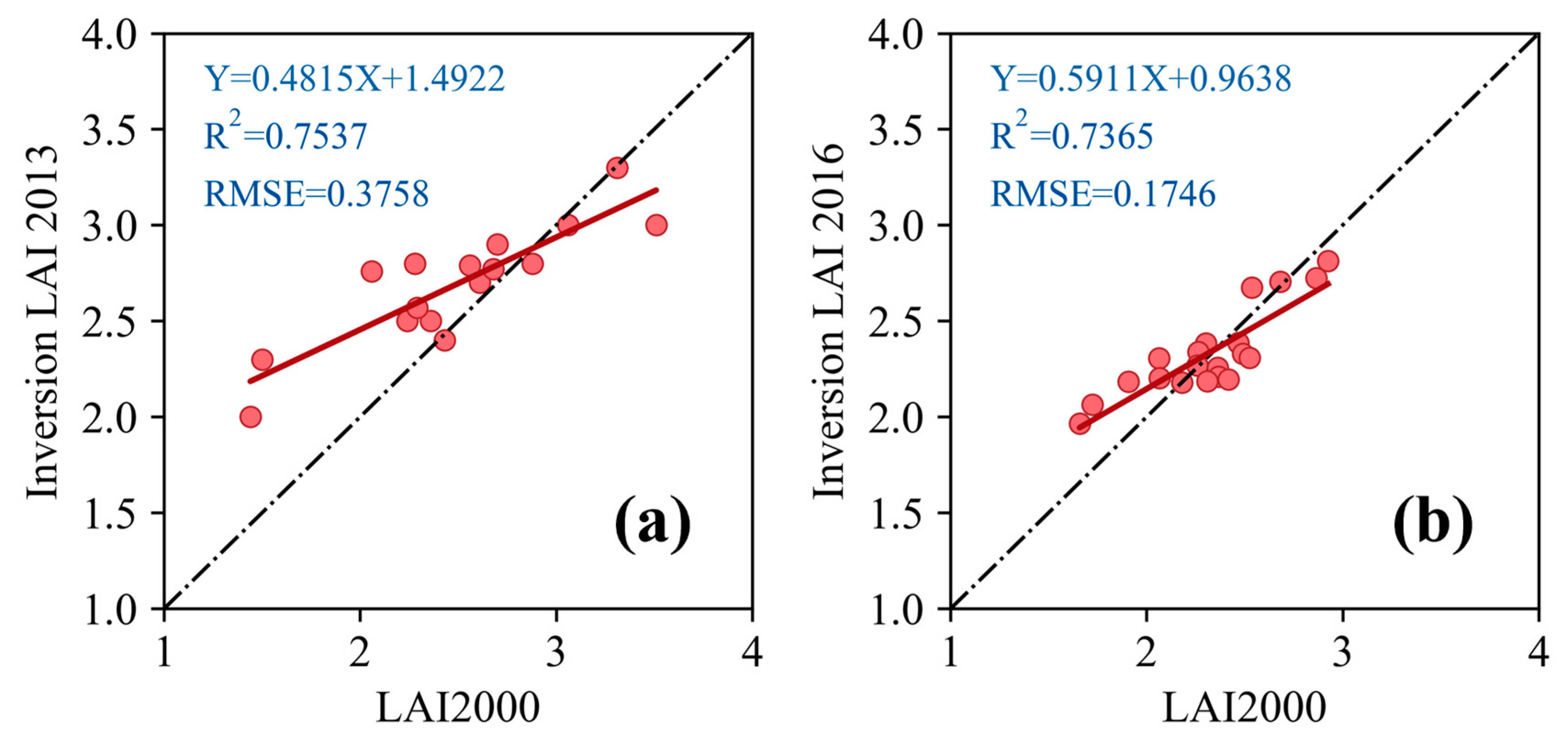
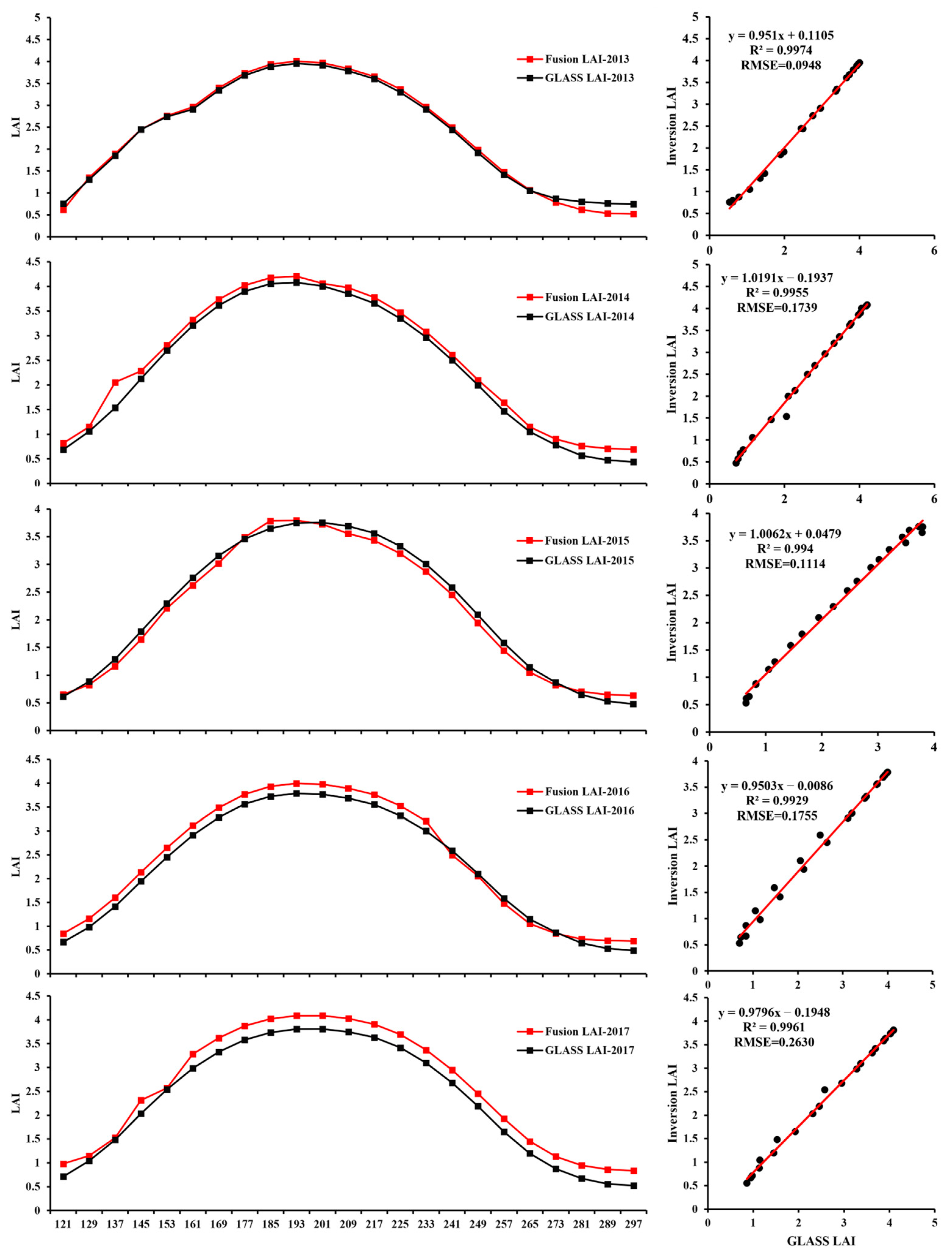
3.1. Inversion LAI Based on SA-BPNN Model

LAI maps retrieved from Landsat8 OLI and GF-1 WFV images were generated using an inversion method based on the SA-BPNN model, and their accuracy was validated through comparison with LAI-2000 ground measurements obtained in situ at the Genhe Ecological Station. Figure 3 shows scatterplots of the LAI measured on the ground in 2013 and 2016 and predicted using the SA-BPNN model. The findings demonstrate a strong positive correlation between the LAI estimated using the SA-BPNN model and the ground-based LAI measurements obtained from the Genhe Ecological Station, indicating the effectiveness of the method in predicting LAI in the study area.

The LAI map predicted from 2013 images (Figure 3a) performed slightly better than the LAI map predicted from 2016 images (Figure 3b), with smaller RMSE and higher R² values (the R² and RMSE of 2013 predicted LAI and observed LAI were 0.7537 and 0.3758, respectively, and 2016 was 0.7365 and 0.1746).

Both Landsat8 OLI and GF-1 WFV images showed good performances in generating LAIs. We compared GF-1 WFV (2013, 2016 and 2017) and Landsat8 OLI (2014 and 2015) images. As described in Section 2.2.3, four bands of the GF-1 WFV image and seven bands of the Landsat8 OLI image were used in the SA-BPNN-based inversion method. The LAI maps were derived by applying an inversion method based on the SA-BPNN model to two satellite datasets, Landsat8 OLI and GF-1 WFV, which were first resampled to the same pixel size (30 m). The consistency of the resulting LAI maps was then evaluated through a comparative analysis. The LAI maps and their difference maps generated using the two sensors during 2013–2017 are shown in Figure 4.

Overall, the LAI prediction surfaces generated using the SA-BPNN model from the Landsat8 OLI and GF-1 WFV images were consistent with the LAI data derived from the GLASS LAI product. In terms of spatial distribution, the retrieved forest vegetation LAI spatiotemporal data show that the southwest region is low, the northeast region is high, and the distribution is scattered from southwest to northeast, which is similar to the distribution of forest vegetation in the study area. However, further analysis of Figure 4 reveals that images from different periods have a significant impact on stitching. Specifically, images from 2013, 2014, and 2016, as well as their corresponding LAI estimations, all contribute to this impact. Additionally, cloud layer inversion for high-resolution vegetation LAI remote sensing may be affected by data pollution in the form of undetected residual thin clouds and cloud shadows on the landscape, which can introduce uncertainty in LAI inversion.

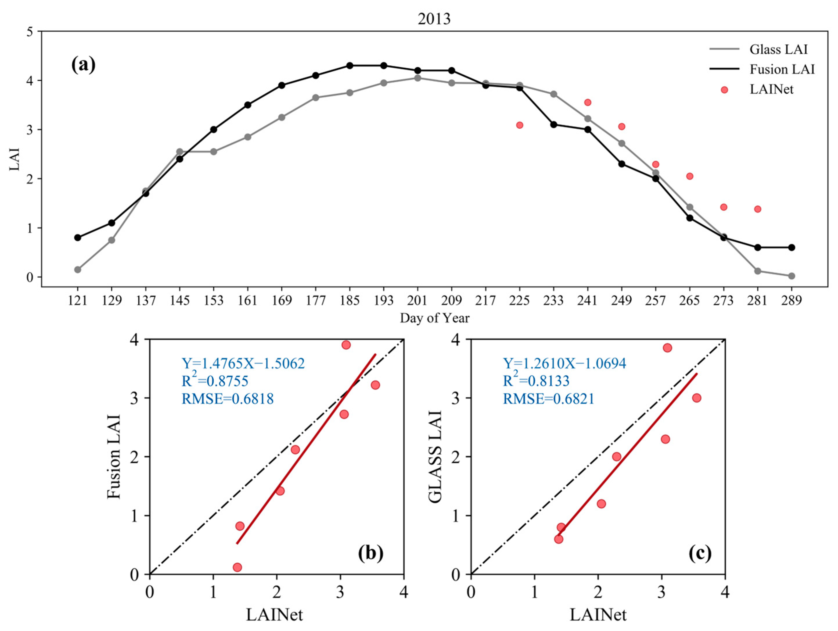
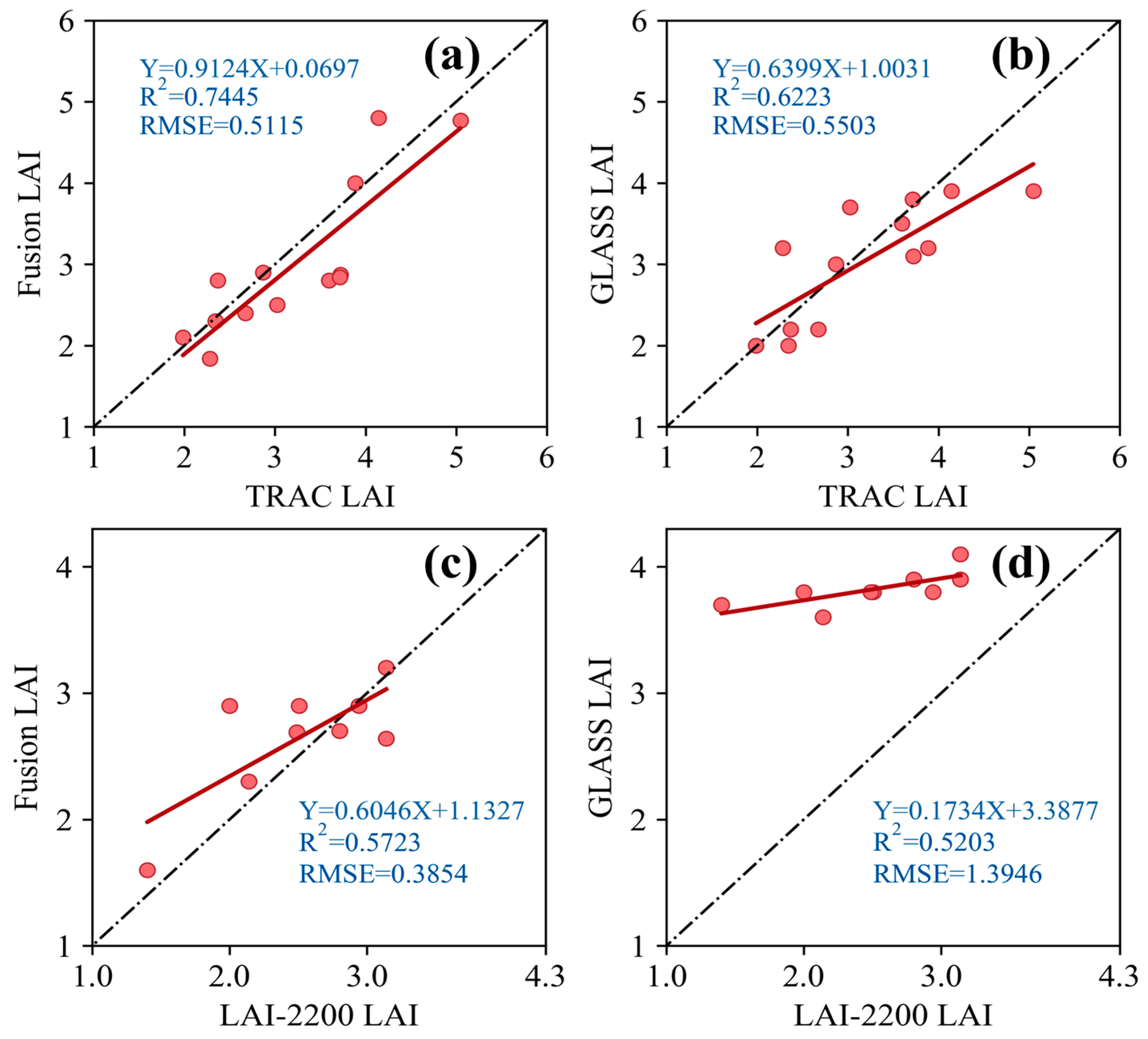
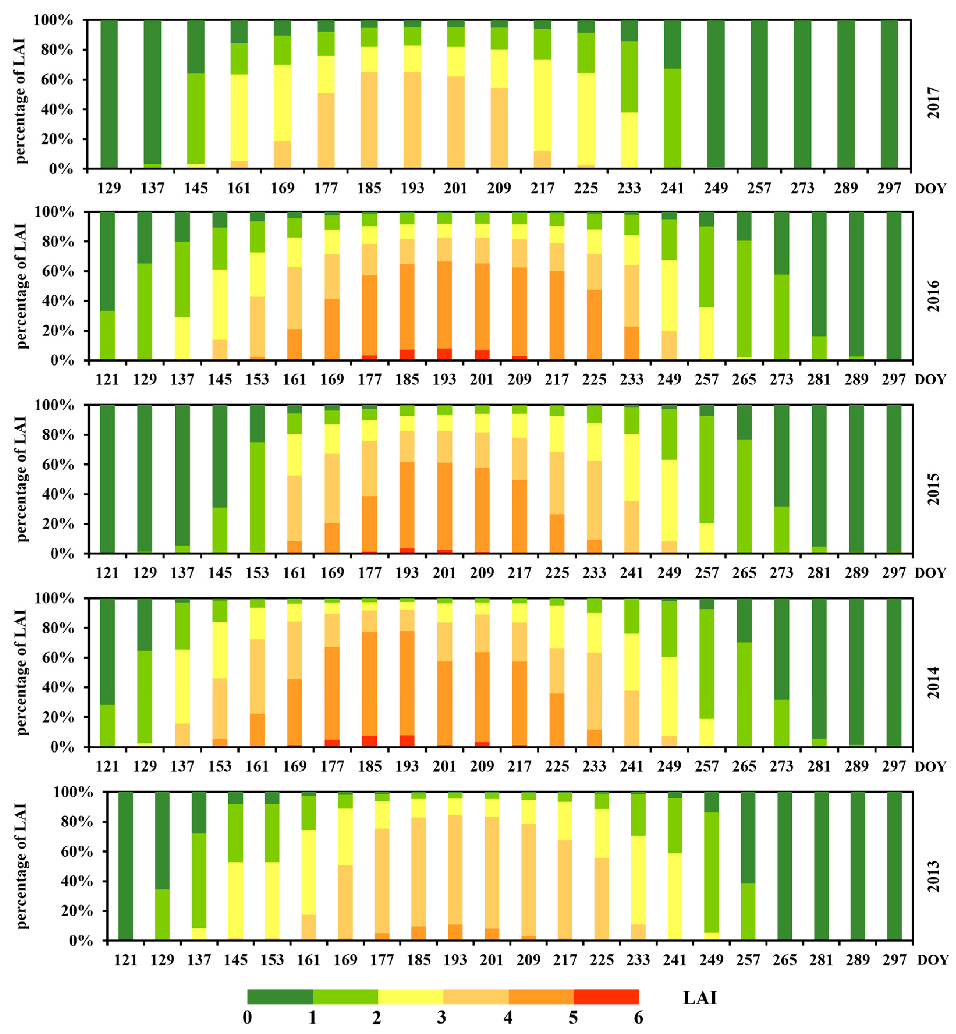
3.2. Time Series of LAI Assimilation

We compared the time series relationship between the fusion LAI and the non-fusion GLASS LAI in the growing season from 2013 to 2017. That is, the average statistics of the fused LAI and the 23 images of the GLASS LAI before the fusion were determined, and the LAI growth season curve every 8 days per year is produced, as shown in Figure 5.

According to the figure, it can be observed that the annual changes in the LAI before and after fusion in 2013–2017 were consistent; that is, the LAI value showed a trend of increasing first and decreasing, and the annual maximum value is also the same. Additionally, this accords with the growth trend of plants in the seasons. For example, from days 193 to 209 in the year, that is, 15–30 July, when plants grow vigorously in summer, the vegetation coverage reaches its highest peak of the year. In the initial period of fusion, that is, from May to June, the leaves of the vegetation are not fully grown and are in the growing period. In the later stage of fusion, that is, from September to October, the growth of vegetation stagnates, and plants are in the leaf defoliation stage, so the LAI was lower and showed a low peak.

It can also be seen from the figure that in the evaluation of the time series relationship between the fused LAI and the non-fusion GLASS LAI from 2013 to 2017, the R² was above 99%. The R² in 2014, 2015 and 2016 was lower, because there were obvious outliers on the 137th day in 2014, the 177–193rd day in 2015, and the 233–257th day in 2016; 2013 and 2017 showed better results than 2014, 2015 and 2016, and the R² was above 99.6% in all years. The results show that the STARFM fusion model based on Landsat8 OLI and GF-1 WFV images obtained LAI products with high temporal and high spatial resolutions, which provides theoretical and technical references for LAI spatiotemporal fusion research based on high-resolution data.

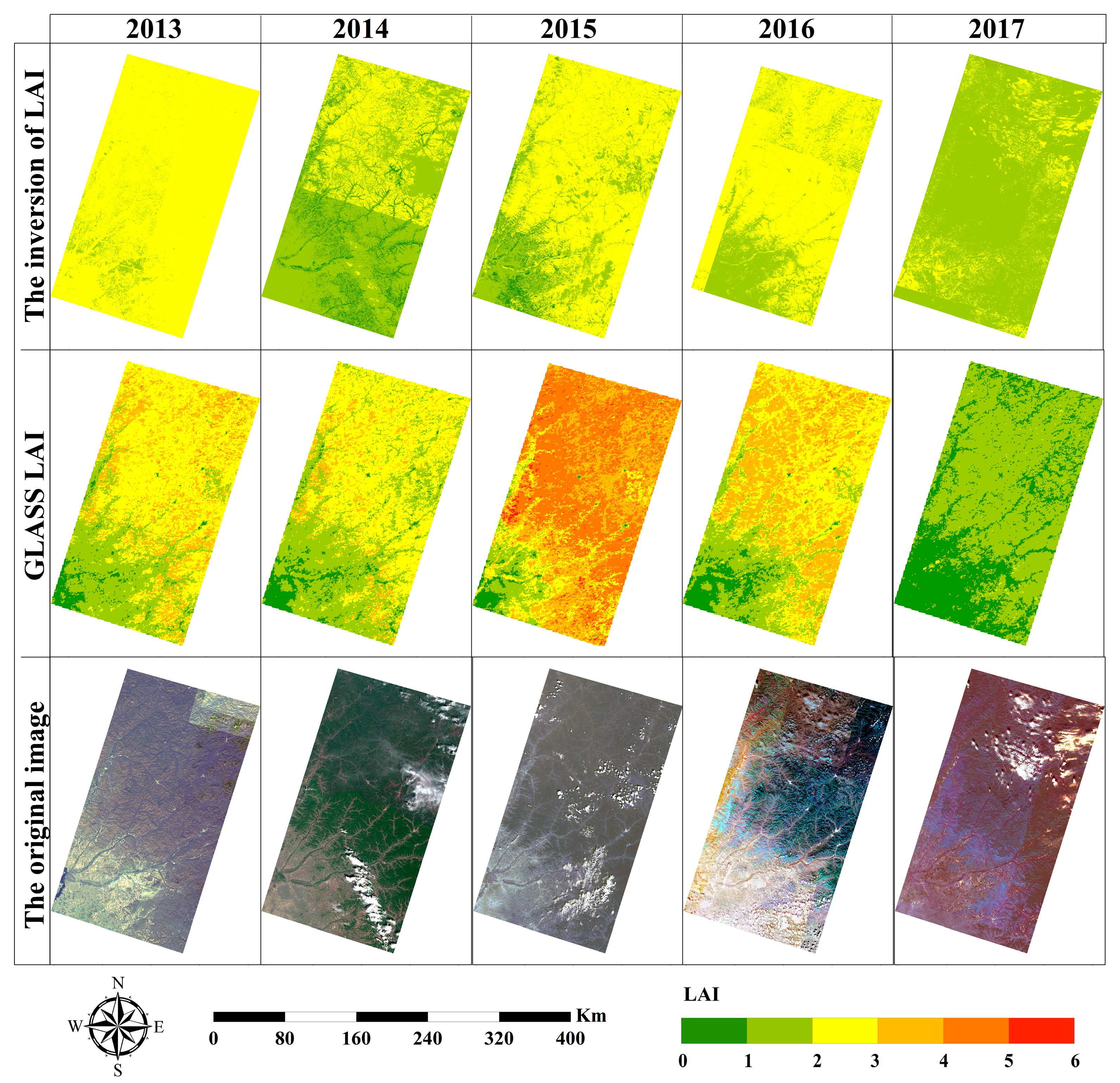
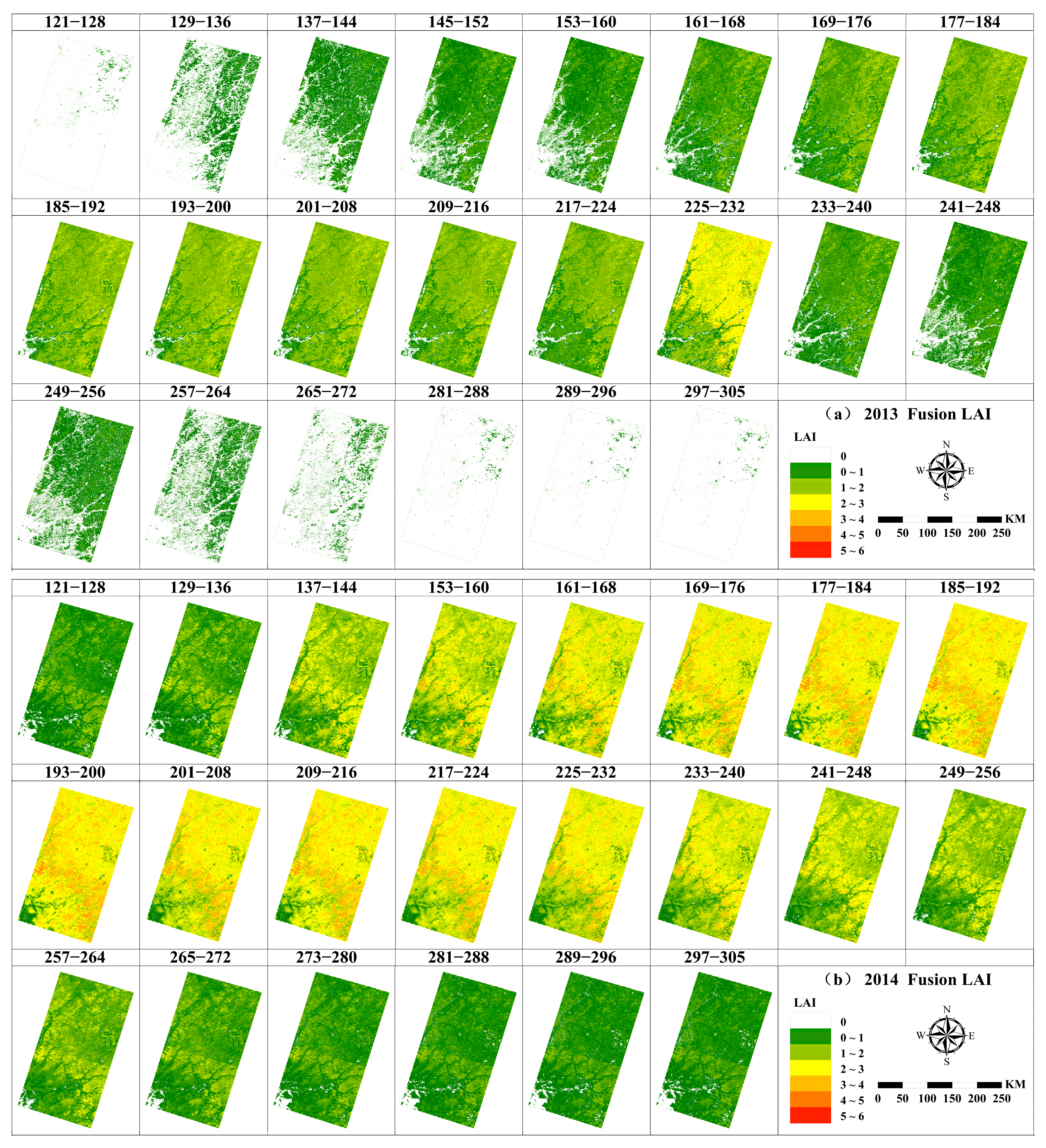
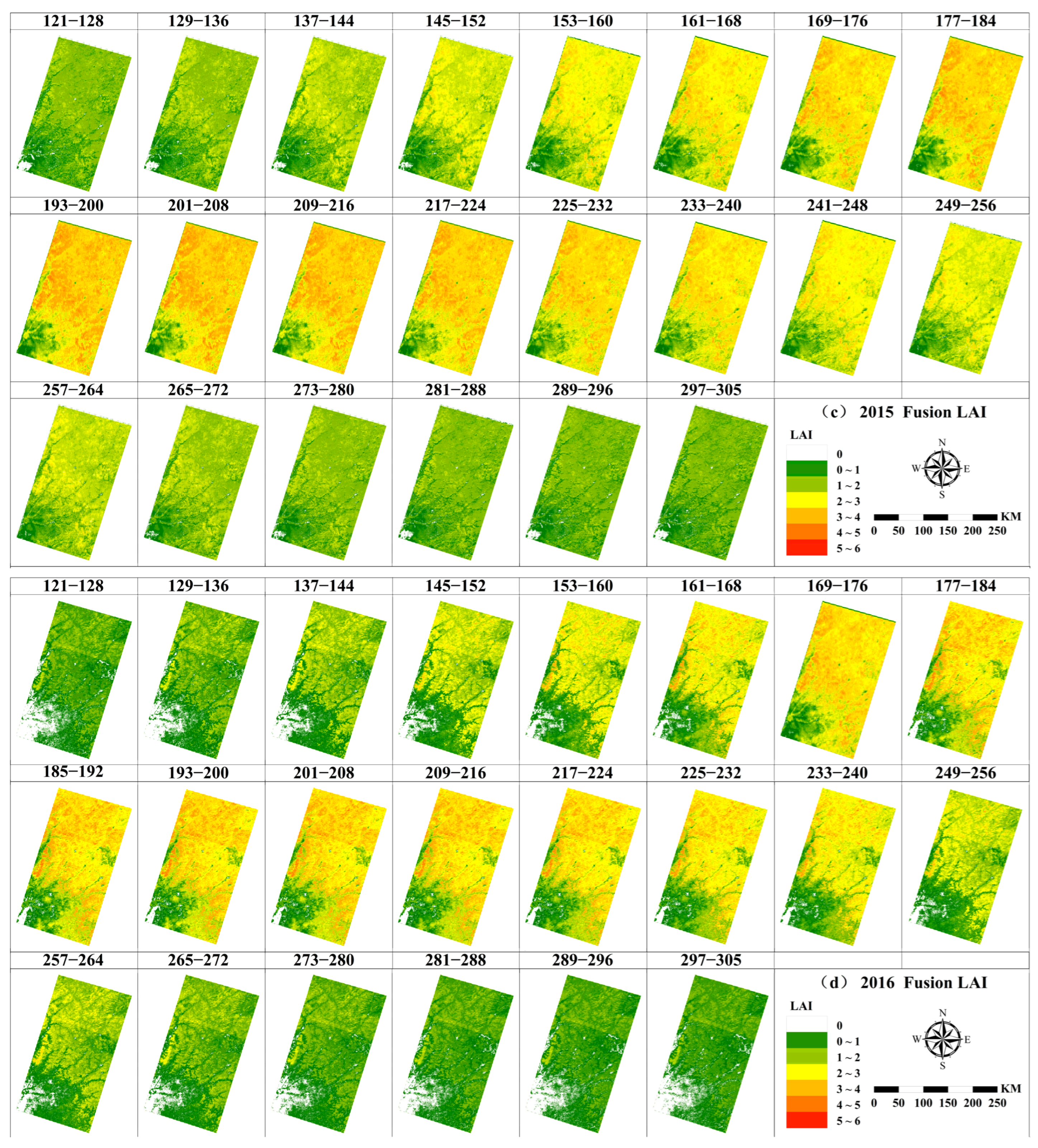
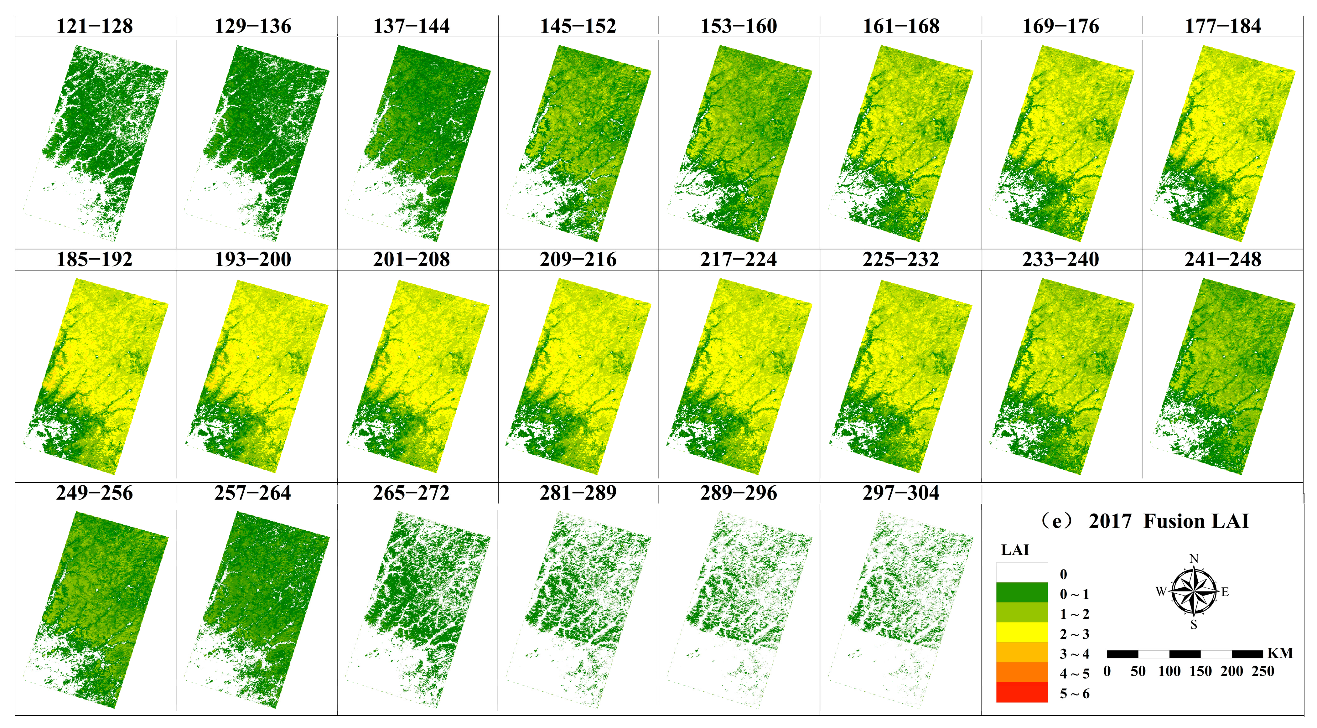
3.3. Spatiotemporal Distribution of LAI Enhancement Methods

Based on the fusion method of the STARFM model, forest stands vegetation growth period (from the 121st to the 305th day of each year) long-term LAI image sequence with a spatial resolution of 30 m and a temporal resolution of 8d in the study area from 2013 to 2017 was generated. The actual survey data in 2013 were used for correlation analysis between LAINet and fusion LAI. The LAINet observation data set of the No. 4 (L3) plot in the Ecological Station of the Genhe Experimental Area (12 August–23 October 2013 was the 233–246th-day instrument failure) and the 65-day daily LAI data of the 225th–297th day were aggregated and averaged every 8 days to form time-series LAI data and correlate with the fused LAI data at the corresponding time in 2013.

Figure 6 and Figure 7 shows the LAI values measured on the ground in 2013, and the LAI fused with the STARFM model, as well as the GLASS correlation scatterplot of the LAI. The correlation analysis between the fused LAI and observed LAI showed a stronger relationship than that between the GLASS LAI and observed LAI. Better R² and lower RMSE values were observed (0.8755 and 0.6818 for fused and survey-observed LAI, and 0.8133 and 0.6821 for GLASS LAI and survey-observed LAI, respectively). The accuracy of the fused LAI was validated using TRAC LAI and LAI-2200 LAI and was found to be superior to GLASS LAI. Overall, these results demonstrate the effectiveness of the proposed method for generating spatiotemporal LAI time series over the study area.

Based on the STARFM fusion model, forest stands vegetation growth period (from the 121st to the 305th day of each year) LAI long-term image series with a spatial resolution of 30 m and temporal resolutions of 8d in the study area from 2013 to 2017 were obtained. The details of the temporal and spatial distribution are shown in Figure 8.

Further analysis of Figure 8 shows that the Spatiotemporal distribution of the fused LAI presented a typical seasonal variation, with lower LAI values in spring and autumn and higher LAI values in summer. During the growing season from May to October: in spring (May), DOY121–145, the LAI value gradually increased; in summer (June–August), DOY145–241, the LAI continued to grow and reached its peak, indicating that the peak period of vegetation growth occurred in during mid- and late July (193–208 days); in autumn (September–October), DOY 242–305, the LAI value decreased gradually. In summary, the fused LAI image was in line with the seasonal growth trend of plants.

4. Discussion

In this study, we estimated stand LAI using Landsat8 OLI and GF-1 WFV reflectance products with the SA-BPNN model. The resulting LAI estimates and GLASS LAI products were fused using the STARFM model to generate time-series LAI products for forest stands during the vegetation growth period from 2013 to 2017, with a temporal resolution of 8 days and a spatial resolution of 30 m.

Fused LAI maps of high spatial resolution long time series were generated using the SA-BPNN model. The results of this study suggest that the LAI maps generated by the SA-BPNN model have demonstrated good performance when compared to ground measurements obtained from the LAI-2000 datasets (Figure 4). In previous studies, the most commonly used method has been to calibrate the PROSAIL radiative transfer model to the specific characteristics of the study area by using background information, and this model can more effectively match the target value range [54,55,56]. However, the PROSAIL radiation transfer model involves a variety of physiological and biochemical parameters and has disadvantages, such as high data acquisition requirements. On the other hand, the SA-BPNN model used in this study has strong nonlinear mapping, high self-learning and self-adaptive abilities, automatically extracts the “reasonable rules” between input and output data through learning, and adaptively memorizes the learning content among the weights of the network; and has strong generalization ability and a certain level of fault tolerance. Furthermore, the effectiveness of the model and inversion strategy has been demonstrated in numerous previous studies, showing that LAI can be successfully retrieved from multitemporal and multiresolution images. Therefore, the model represents a new idea for forest vegetation LAI inversion.

STARFM aims to generate 30 m spatial resolution and 8d LAI by fusing time-sparse Landsat8 OLI LAI and GF-1 WFV LAI images with collected high temporal resolution GLASS LAI images. Divide the LAI assimilated each year from 2013 to 2017 into six levels, and obtain the corresponding LAI histogram (Figure 9). The results show that the histogram of assimilated LAI also shows the same pattern. Specifically, during spring and winter, the majority of the LAI values were low, while during summer and early autumn, there was a significant increase in the proportion of high LAI values. In addition, the assimilated average LAI from 2013 to 2017 (Figure 5) is consistent with the changing trend in the LAI histogram corresponding to each year (Figure 9). This result suggests that the assimilated LAI effectively captures the spatial and temporal dynamics of forest vegetation LAI. In this study, it was successfully used to fuse the LAI product generated using the SA-BPNN model. By utilizing a method that searches for pixels with similar spectral characteristics within a moving window, the generated high spatiotemporal-resolution images successfully captured the temporal variation in the GLASS LAI time series while maintaining the high-resolution spatial details found in both the Landsat8 OLI LAI and GF-1 WFV LAI images.

A uniform seasonal distribution of sharp high-spatial-resolution scale images is another important requirement for achieving good performance with the STARFM algorithm. In areas with frequent cloud cover, Landsat8 OLI images alone are insufficient to capture temporal changes in forest vegetation. The addition of high-spatial-resolution GF-1 WFV images provides additional temporal information and improves the ability to detect changes in canopy structure. In this study, combining high spatial resolution GF-1 WFV and Landsat8 OLI data with GLASS LAI data can provide more detailed spatial information and effectively increase the high spatial resolution. However, this study also found the significant impact of cloud cover on the accuracy of the STARFM model during vegetation parameter estimation and fusion. Cloud cover can cause pixel distortion, making it challenging for the model to extract vegetation parameter information from remote sensing data accurately. Furthermore, it can result in data loss, further reducing the accuracy of the model. Therefore, it is crucial to address cloud cover by using cloud masks, cloud restoration algorithms, etc., to minimize its impact on the model in future research when applying the STARFM model to estimate vegetation parameters. Previous studies have also demonstrated that the STARFM model may encounter significant prediction errors when estimating vegetation parameters in small areas if no pure-sized pixels are found in the search window [25,57], as observed in this study. Furthermore, the STARFM model can eliminate most of the abnormal points in the original LAI curve; a small number of abnormal fluctuations in the LAI time series may still lead to uncertainty in the spline interpolation and result in a less smooth LAI curve. To overcome this challenge, future research can employ higher spatial resolution vegetation datasets, which may help identify purer coarse-resolution neighboring pixels and reduce prediction errors in vegetation parameters within small areas. Alternatively, future research could explore the use of more advanced time series data algorithms to replace missing or poorly observed values and generate temporally smooth and spatially complete datasets. This approach can lead to more accurate prediction results, improving the overall performance of the model.

5. Conclusions

In this study, we utilized multisource remote sensing ground reflectance data from Landsat8 OLI and GF-1 WFV to construct an SA-BPNN model for LAI estimation in the study area. Subsequently, we employed the STARFM to integrate the GLAAS LAI product with the high-spatial-resolution LAI data estimated from Landsat8 OLI and GF-1 WFV. By doing so, we generated a time-series product of forest stand vegetation growth (LAI) during the growth period (121^st to 305^th day of each year) with a temporal resolution of 8 days and a spatial resolution of 30 m. The results show the following: (1) The SA-BPNN estimation model had high precision (the estimated values of the 2013 LAI model were R² = 0.7537 and RMSE = 0.3758; the estimated values of the 2016 LAI model were R² = 0.7365 and RMSE = 0.1746); (2) After fusion, the 30 m LAI product had good correlation with the LAI verification of the measured sample site (R² = 0.8775); compared with the GLASS LAI interannual trend line in the same time period Same result (R² = 0.8133). The results indicate that combining ground reflectance data from Landsat 8 OLI and GF-1 WFV sensors enhances LAI estimation and expands the range of available data for analysis. These findings provide a valuable reference for future research on the spatiotemporal fusion of LAI with high-resolution domestic data. The high-temporal and high-spatial-resolution LAI products generated in this study offer critical data to facilitate investigations into changes in carbon cycles.

References

1. Chen, J.M.; Black, T.A. Defining Leaf Area Index for Non-Flat Leaves. Plant Cell Environ. 1992, 15, 421–429. [Google Scholar] [CrossRef]
2. Bonan, G.B. Importance of Leaf Area Index and Forest Type When Estimating Photosynthesis in Boreal Forests. Remote Sens. Environ. 1993, 43, 303–314. [Google Scholar] [CrossRef]
3. Asner, G.P.; Scurlock, J.M.O.; Hicke, J.A. Global Synthesis of Leaf Area Index Observations: Implications for Ecological and Remote Sensing Studies. Glob. Ecol. Biogeogr. 2003, 12, 191–205. [Google Scholar] [CrossRef]
4. Sellers, P.J.; Dickinson, R.E.; Randall, D.A.; Betts, A.K.; Hall, F.G.; Berry, J.A.; Collatz, G.J.; Denning, A.S.; Mooney, H.A.; Nobre, C.A.; et al. Modeling the Exchanges of Energy, Water, and Carbon Between Continents and the Atmosphere. Science 1997, 275, 502–509. Available online: https://www.science.org/doi/abs/10.1126/science.275.5299.502 (accessed on 30 November 2022). [CrossRef]
5. Colombo, R.; Bellingeri, D.; Fasolini, D.; Marino, C.M. Retrieval of Leaf Area Index in Different Vegetation Types Using High Resolution Satellite Data. Remote Sens. Environ. 2003, 86, 120–131. [Google Scholar] [CrossRef]
6. Houborg, R.; McCabe, M.F.; Gao, F. A Spatio-Temporal Enhancement Method for Medium Resolution LAI (STEM-LAI). Int. J. Appl. Earth Obs. Geoinf. 2016, 47, 15–29. [Google Scholar] [CrossRef]
7. Campos-Taberner, M.; García-Haro, F.J.; Camps-Valls, G.; Grau-Muedra, G.; Nutini, F.; Crema, A.; Boschetti, M. Multitemporal and Multiresolution Leaf Area Index Retrieval for Operational Local Rice Crop Monitoring. Remote Sens. Environ. 2016, 187, 102–118. [Google Scholar] [CrossRef]
8. Xu, J.; Quackenbush, L.J.; Volk, T.A.; Im, J. Forest and Crop Leaf Area Index Estimation Using Remote Sensing: Research Trends and Future Directions. Remote Sens. 2020, 12, 2934. [Google Scholar] [CrossRef]
9. Paoletti, M.E.; Haut, J.M.; Plaza, J.; Plaza, A. Deep Learning Classifiers for Hyperspectral Imaging: A Review. ISPRS J. Photogramm. Remote Sens. 2019, 158, 279–317. [Google Scholar] [CrossRef]
10. Zhang, H.; Ma, J.; Chen, C.; Tian, X. NDVI-Net: A Fusion Network for Generating High-Resolution Normalized Difference Vegetation Index in Remote Sensing. ISPRS J. Photogramm. Remote Sens. 2020, 168, 182–196. [Google Scholar] [CrossRef]
11. Wang, W.; Ma, Y.; Meng, X.; Sun, L.; Jia, C.; Jin, S.; Li, H. Retrieval of the Leaf Area Index from MODIS Top-of-Atmosphere Reflectance Data Using a Neural Network Supported by Simulation Data. Remote Sens. 2022, 14, 2456. [Google Scholar] [CrossRef]
12. Nandan, R.; Bandaru, V.; He, J.; Daughtry, C.; Gowda, P.; Suyker, A.E. Evaluating Optical Remote Sensing Methods for Estimating Leaf Area Index for Corn and Soybean. Remote Sens. 2022, 14, 5301. [Google Scholar] [CrossRef]
13. Zhang, G.; Ma, H.; Liang, S.; Jia, A.; He, T.; Wang, D. A Machine Learning Method Trained by Radiative Transfer Model Inversion for Generating Seven Global Land and Atmospheric Estimates from VIIRS Top-of-Atmosphere Observations. Remote Sens. Environ. 2022, 279, 113132. [Google Scholar] [CrossRef]
14. Li, J.; Xiao, Z.; Sun, R.; Song, J. Retrieval of the Leaf Area Index from Visible Infrared Imaging Radiometer Suite (VIIRS) Surface Reflectance Based on Unsupervised Domain Adaptation. Remote Sens. 2022, 14, 1826. [Google Scholar] [CrossRef]
15. Min, Y.; Jie, L.; Gu, Z.; Tong, G.; Yongbing, W.; Zhang, J.; Lu, X. Leaf Area Index Retrieval Based on Landsat 8 OLI Multi-Spectral Image Data and BP Neural Network. Sswcc 2015, 8, 86–93. [Google Scholar]
16. Zhu, D.E.; Xu, X.J.; Du, H.Q.; Zhou, G.M.; Mao, F.J.; Li, X.J.; Li, Y.G. Retrieval of leaf area index of Phyllostachys praecox forest based on MODIS reflectance time series data. J. Appl. Ecol. 2018, 29, 2391–2400. [Google Scholar] [CrossRef]
17. Liu, B.; Wang, R.; Zhao, G.; Guo, X.; Wang, Y.; Li, J.; Wang, S. Prediction of Rock Mass Parameters in the TBM Tunnel Based on BP Neural Network Integrated Simulated Annealing Algorithm. Tunn. Undergr. Space Technol. 2020, 95, 103103. [Google Scholar] [CrossRef]
18. Zhou, H.; Wang, C.; Zhang, G.; Xue, H.; Wang, J.; Wan, H. Generating a Spatio-Temporal Complete 30 m Leaf Area Index from Field and Remote Sensing Data. Remote Sens. 2020, 12, 2394. [Google Scholar] [CrossRef]
19. Li, K.; Zhang, W.; Yu, D.; Tian, X. HyperNet: A Deep Network for Hyperspectral, Multispectral, and Panchromatic Image Fusion. ISPRS J. Photogramm. Remote Sens. 2022, 188, 30–44. [Google Scholar] [CrossRef]
20. Liu, P.; Li, J.; Wang, L.; He, G. Remote Sensing Data Fusion With Generative Adversarial Networks: State-of-the-Art Methods and Future Research Directions. IEEE Geosci. Remote Sens. Mag. 2022, 10, 295–328. [Google Scholar] [CrossRef]
21. Xu, F.; Liu, J.; Song, Y.; Sun, H.; Wang, X. Multi-Exposure Image Fusion Techniques: A Comprehensive Review. Remote Sens. 2022, 14, 771. [Google Scholar] [CrossRef]
22. Azarang, A.; Kehtarnavaz, N. A Generative Model Method for Unsupervised Multispectral Image Fusion in Remote Sensing. SIViP 2022, 16, 63–71. [Google Scholar] [CrossRef]
23. Wen, J.; Wu, X.; You, D.; Ma, X.; Ma, D.; Wang, J.; Xiao, Q. The Main Inherent Uncertainty Sources in Trend Estimation Based on Satellite Remote Sensing Data. Appl. Clim. 2022, 151, 915–934. [Google Scholar] [CrossRef]
24. Wen, J.; Wu, X.; Wang, J.; Tang, R.; Ma, D.; Zeng, Q.; Gong, B.; Xiao, Q. Characterizing the Effect of Spatial Heterogeneity and the Deployment of Sampled Plots on the Uncertainty of Ground “Truth” on a Coarse Grid Scale: Case Study for Near-Infrared (NIR) Surface Reflectance. J. Geophys. Res. Atmos. 2022, 127, e2022JD036779. [Google Scholar] [CrossRef]
25. Gao, F.; Masek, J.; Schwaller, M.; Hall, F. On the Blending of the Landsat and MODIS Surface Reflectance: Predicting Daily Landsat Surface Reflectance. IEEE Trans. Geosci. Remote Sens. 2006, 44, 2207–2218. [Google Scholar] [CrossRef]
26. Gevaert, C.M.; García-Haro, F.J. A Comparison of STARFM and an Unmixing-Based Algorithm for Landsat and MODIS Data Fusion. Remote Sens. Environ. 2015, 156, 34–44. [Google Scholar] [CrossRef]
27. Yuan, Z.; Zhang, J. Fusion of Spatiotemporal Remote sensing Data for Changing Surface Characteristics. J. Beijing Norm. Univ. (Nat. Sci.) 2017, 53, 727–734. [Google Scholar]
28. Tao, G.; Jia, K.; Zhao, X.; Wei, X.; Xie, X.; Zhang, X.; Wang, B.; Yao, Y.; Zhang, X. Generating High Spatio-Temporal Resolution Fractional Vegetation Cover by Fusing GF-1 WFV and MODIS Data. Remote Sens. 2019, 11, 2324. [Google Scholar] [CrossRef]
29. Wang, S.; Yang, X.; Li, G.; Jin, Y.; Tian, C. Research on Spatio-Temporal Fusion Algorithm of Remote Sensing Image Based on GF-1 WFV and Sentinel-2 Satellite Data. In Proceedings of the 2022 3rd International Conference on Geology, Mapping and Remote Sensing (ICGMRS), Zhousan, China, 22–24 April 2022; pp. 667–678. [Google Scholar]
30. Wen, J.; Lin, X.; Wu, X.; Bao, Y.; You, D.; Gong, B.; Tang, Y.; Wu, S.; Xiao, Q.; Liu, Q. Validation of the MCD43A3 Collection 6 and GLASS V04 Snow-Free Albedo Products Over Rugged Terrain. IEEE Trans. Geosci. Remote Sens. 2022, 60, 1–11. [Google Scholar] [CrossRef]
31. Chen, B.; Xu, B.; Zhu, Z.; Yuan, C.; Suen, H.P.; Guo, J.; Xu, N.; Li, W.; Zhao, Y.; Yang, J. Stable Classification with Limited Sample: Transferring a 30-m Resolution Sample Set Collected in 2015 to Mapping 10-m Resolution Global Land Cover in 2017. Sci. Bull. 2019, 64, 370–373. [Google Scholar] [CrossRef]
32. Xiang, Y.; Xiao, Z.Q.; Liang, S.; Wang, J.D.; Song, J.L. Validation of Global LAnd Surface Satellite (GLASS) Leaf Area Index Product. J. Remote Sens. 2014, 18, 573–596. [Google Scholar] [CrossRef]
33. Singla, J.G.; Trivedi, S. Generation of State of the Art Very High Resolution DSM over Hilly Terrain Using Cartosat-2 Multi-View Data, Its Comparison and Evaluation–A Case Study near Alwar Region. J. Geomat. 2022, 16, 23–32. [Google Scholar]
34. Li, X.; Wang, T.; Cui, H.; Zhang, G.; Cheng, Q.; Dong, T.; Jiang, B. SARPointNet: An Automated Feature Learning Framework for Spaceborne SAR Image Registration. IEEE J. Sel. Top. Appl. Earth Obs. Remote Sens. 2022, 15, 6371–6381. [Google Scholar] [CrossRef]
35. Bin, W.; Ming, L.; Dan, J.; Suju, L.; Qiang, C.; Chao, W.; Yang, Z.; Huan, Y.; Jun, Z. A Method of Automatically Extracting Forest Fire Burned Areas Using Gf-1 Remote Sensing Images. In Proceedings of the IGARSS 2019–2019 IEEE International Geoscience and Remote Sensing Symposium, Yokohama, Japan, 28 July 2019; pp. 9953–9955. [Google Scholar]
36. Kong, Z.; Yang, H.; Zheng, F.; Yang, Z.; Li, Y.; Qi, J. Atmospheric Correction Assessment for GF-1 WFV. In Proceedings of the International Conference on Environmental Remote Sensing and Big Data (ERSBD 2021), Wuhan, China, 9 December 2021; SPIE: Bellingham, WA, USA, 2021; Volume 12129, pp. 270–275. [Google Scholar]
37. Han, W.; Chen, D.; Li, H.; Chang, Z.; Chen, J.; Ye, L.; Liu, S.; Wang, Z. Spatiotemporal Variation of NDVI in Anhui Province from 2001 to 2019 and Its Response to Climatic Factors. Forests 2022, 13, 1643. [Google Scholar] [CrossRef]
38. Li, S.; Zhang, R.; Xie, L.; Zhan, J.; Song, Y.; Zhan, R.; Shama, A.; Wang, T. A Factor Analysis Backpropagation Neural Network Model for Vegetation Net Primary Productivity Time Series Estimation in Western Sichuan. Remote Sens. 2022, 14, 3961. [Google Scholar] [CrossRef]
39. Hecht-nielsen, R. III.3–Theory of the Backpropagation Neural Network. In Neural Networks for Perception; Wechsler, H., Ed.; Academic Press: Cambridge, MA, USA, 1992; pp. 65–93. ISBN 978-0-12-741252-8. [Google Scholar]
40. Zhang, Y.; Hu, Q.; Li, H.; Li, J.; Liu, T.; Chen, Y.; Ai, M.; Dong, J. A Back Propagation Neural Network-Based Radiometric Correction Method (BPNNRCM) for UAV Multispectral Image. IEEE J. Sel. Top. Appl. Earth Obs. Remote Sens. 2023, 16, 112–125. [Google Scholar] [CrossRef]
41. Fan, Y.; Li, G.; Wu, J. Research on Monitoring Overground Carbon Stock of Forest Vegetation Communities Based on Remote Sensing Technology. Proc. Indian Natl. Sci. Acad. 2022, 88, 705–713. [Google Scholar] [CrossRef]
42. Smith, J.A. LAI Inversion Using a Back-Propagation Neural Network Trained with a Multiple Scattering Model. IEEE Trans. Geosci. Remote Sens. 1993, 31, 1102–1106. [Google Scholar] [CrossRef]
43. Li, L.; Chen, Y.; Xu, T.; Liu, R.; Shi, K.; Huang, C. Super-Resolution Mapping of Wetland Inundation from Remote Sensing Imagery Based on Integration of Back-Propagation Neural Network and Genetic Algorithm. Remote Sens. Environ. 2015, 164, 142–154. [Google Scholar] [CrossRef]
44. Xu, S.; Li, S.; Tao, Z.; Song, K.; Wen, Z.; Li, Y.; Chen, F. Remote Sensing of Chlorophyll-a in Xinkai Lake Using Machine Learning and GF-6 WFV Images. Remote Sens. 2022, 14, 5136. [Google Scholar] [CrossRef]
45. Miao, Y.; Zhang, R.; Guo, J.; Yi, S.; Meng, B.; Liu, J. Vegetation Coverage in the Desert Area of the Junggar Basin of Xinjiang, China, Based on Unmanned Aerial Vehicle Technology and Multisource Data. Remote Sens. 2022, 14, 5146. [Google Scholar] [CrossRef]
46. Metropolis, N.; Rosenbluth, A.W.; Rosenbluth, M.N.; Teller, A.H.; Teller, E. Equation of State Calculations by Fast Computing Machines. J. Chem. Phys. 1953, 21, 1087–1092. [Google Scholar] [CrossRef]
47. Li, J.; Tian, L.; Wang, Y.; Jin, S.; Li, T.; Hou, X. Optimal Sampling Strategy of Water Quality Monitoring at High Dynamic Lakes: A Remote Sensing and Spatial Simulated Annealing Integrated Approach. Sci. Total Environ. 2021, 777, 146113. [Google Scholar] [CrossRef]
48. Yang, P.; Hu, J.; Hu, B.; Luo, D.; Peng, J. Estimating Soil Organic Matter Content in Desert Areas Using In Situ Hyperspectral Data and Feature Variable Selection Algorithms in Southern Xinjiang, China. Remote Sens. 2022, 14, 5221. [Google Scholar] [CrossRef]
49. Xue, H.; Wang, C.; Zhou, H.; Wang, J.; Wan, H. BP Neural Network Based on Simulated Annealing Algorithm for High Resolution LAI Retrieval. Remote Sens. Technol. Appl. 2020, 35, 1057–1069. [Google Scholar]
50. Cao, Y.; Du, P.; Zhang, M.; Bai, X.; Lei, R.; Yang, X. Quantitative Evaluation of Grassland SOS Estimation Accuracy Based on Different MODIS-Landsat Spatio-Temporal Fusion Datasets. Remote Sens. 2022, 14, 2542. [Google Scholar] [CrossRef]
51. Meng, X.; Liu, Q.; Shao, F.; Li, S. Spatio–Temporal–Spectral Collaborative Learning for Spatio–Temporal Fusion with Land Cover Changes. IEEE Trans. Geosci. Remote Sens. 2022, 60, 1–16. [Google Scholar] [CrossRef]
52. Yang, Y.; Anderson, M.C.; Gao, F.; Hain, C.R.; Semmens, K.A.; Kustas, W.P.; Noormets, A.; Wynne, R.H.; Thomas, V.A.; Sun, G. Daily Landsat-Scale Evapotranspiration Estimation over a Forested Landscape in North Carolina, USA, Using Multi-Satellite Data Fusion. Hydrol. Earth Syst. Sci. 2017, 21, 1017–1037. [Google Scholar] [CrossRef]
53. Yin, G.; Li, A.; Jin, H.; Zhao, W.; Bian, J.; Qu, Y.; Zeng, Y.; Xu, B. Derivation of Temporally Continuous LAI Reference Maps through Combining the LAINet Observation System with CACAO. Agric. For. Meteorol. 2017, 233, 209–221. [Google Scholar] [CrossRef]
54. Combal, B.; Baret, F.; Weiss, M.; Trubuil, A.; Macé, D.; Pragnère, A.; Myneni, R.; Knyazikhin, Y.; Wang, L. Retrieval of Canopy Biophysical Variables from Bidirectional Reflectance: Using Prior Information to Solve the Ill-Posed Inverse Problem. Remote Sens. Environ. 2003, 84, 1–15. [Google Scholar] [CrossRef]
55. Si, Y.; Schlerf, M.; Zurita-Milla, R.; Skidmore, A.; Wang, T. Mapping Spatio-Temporal Variation of Grassland Quantity and Quality Using MERIS Data and the PROSAIL Model. Remote Sens. Environ. 2012, 121, 415–425. [Google Scholar] [CrossRef]
56. Campos-Taberner, M.; García-Haro, F.J.; Camps-Valls, G.; Grau-Muedra, G.; Nutini, F.; Busetto, L.; Katsantonis, D.; Stavrakoudis, D.; Minakou, C.; Gatti, L.; et al. Exploitation of SAR and Optical Sentinel Data to Detect Rice Crop and Estimate Seasonal Dynamics of Leaf Area Index. Remote Sens. 2017, 9, 248. [Google Scholar] [CrossRef]
57. Gao, F.; Hilker, T.; Zhu, X.; Anderson, M.; Masek, J.; Wang, P.; Yang, Y. Fusing Landsat and MODIS Data for Vegetation Monitoring. IEEE Geosci. Remote Sens. Mag. 2015, 3, 47–60. [Google Scholar] [CrossRef]
Figure 1. Location of the study area and the actual observation point of the plot. (a) Inner Mongolia Autonomous Region of China; (b) land use data in the research area; (c) GLASS LAI local area; (d) Landsat8 OLI remote sensing image; and (e) GF-1 WFV remote sensing image.
Remotesensing 15 02812 g001
Figure 2. The technical framework of this study.
Remotesensing 15 02812 g002
Figure 3. Based on SA-BPNN LAI measured value and inversion value correlation: (a) observations of LAI-2000 plots in 2013; (b) observations of LAI-2000 plots in 2016.
Remotesensing 15 02812 g003
Figure 4. Estimated LAI results of the SA-BPNN model from 2013 to 2017.
Remotesensing 15 02812 g004
Figure 5. LAI curve of the fusion image every 8 days during the mean value of stand LAI growing season from 2013 to 2017 and its comparison with the mean value of GLASS LAI.
Remotesensing 15 02812 g005
Figure 6. The relationships between (a) Fusion LAI, GLASS LAI and LAINet LAI, and the comparison of (b) Fusion LAI, and (c) GLASS LAI and LAINet LAI.
Remotesensing 15 02812 g006
Figure 7. The relationships between Fusion LAI, GLASS LAI and TRAC LAI, LAI-2200 LAI, and the comparison of (a) Fusion LAI, (b) GLASS LAI and TRAC LAI; and (c) Fusion LAI, (d) GLASS LAI and LAI-2200 LAI.
Remotesensing 15 02812 g007
Figure 8. Spatiotemporal distributions of time-series LAI assimilation of forest stand vegetation in research area during 2013–2017. (a) Fusion LAI results in the GF-1 WFV growing season 2013; (b) Fusion LAI results in the Landsat8 OLI growing season 2014; (c) Fusion LAI results in the Landsat8 OLI growing season 2015; (d) Fusion LAI results in the GF-1 WFV growing season 2016; and (e) Fusion LAI results in the GF-1 WFV growing season 2017.
Remotesensing 15 02812 g008aRemotesensing 15 02812 g008bRemotesensing 15 02812 g008c
Figure 9. Statistical histogram of 2013–2017 fusion LAI values.
Remotesensing 15 02812 g009