Estimating Snow Depth and Leaf Area Index Based on UAV Digital Photogrammetry


Department of Physical Geography and Geoecology, Faculty of Science, Charles University, Albertov 6, 128 43 Prague, Czech Republic
*
Author to whom correspondence should be addressed.
Sensors 2019, 19(5), 1027; https://0-doi-org.brum.beds.ac.uk/10.3390/s19051027
Submission received: 17 December 2018
/
Revised: 20 February 2019
/
Accepted: 23 February 2019
/
Published: 28 February 2019
(This article belongs to the Special Issue Unmanned Aerial Vehicles in Earth and Environmental Sciences)
Abstract
:This study presents a novel approach in the application of Unmanned Aerial Vehicle (UAV) imaging for the conjoint assessment of the snow depth and winter leaf area index (LAI), a structural property of vegetation, affecting the snow accumulation and snowmelt. The snow depth estimation, based on a multi-temporal set of high-resolution digital surface models (DSMs) of snow-free and of snow-covered conditions, taken in a partially healthy to insect-induced Norway spruce forest and meadow coverage area within the Šumava National Park (Šumava NP) in the Czech Republic, was assessed over a winter season. The UAV-derived DSMs featured a resolution of 0.73–1.98 cm/pix. By subtracting the DSMs, the snow depth was determined and compared with manual snow probes taken at ground control point (GCP) positions, the root mean square error (RMSE) ranged between 0.08 m and 0.15 m. A comparative analysis of UAV-based snow depth with a denser network of arranged manual snow depth measurements yielded an RMSE between 0.16 m and 0.32 m. LAI assessment, crucial for correct interpretation of the snow depth distribution in forested areas, was based on downward-looking UAV images taken in the forest regime. To identify the canopy characteristics from downward-looking UAV images, the snow background was used instead of the sky fraction. Two conventional methods for the effective winter LAI retrieval, the LAI-2200 plant canopy analyzer, and digital hemispherical photography (DHP) were used as a reference. Apparent was the effect of canopy density and ground properties on the accuracy of DSMs assessment based on UAV imaging when compared to the field survey. The results of UAV-based LAI values provided estimates were comparable to values derived from the LAI-2200 plant canopy analyzer and DHP. Comparison with the conventional survey indicated that spring snow depth was overestimated, and spring LAI was underestimated by using UAV photogrammetry method. Since the snow depth and the LAI parameters are essential for snowpack studies, this combined method here will be of great value in the future to simplify snow depth and LAI assessment of snow dynamics.
1. Introduction
Snow is an essential component of the hydrological cycle [1]. It serves as a reliable water resource and the dynamics of snow cover play a vital function in rebalancing the global energy and water budget [2]. Due to the unique characteristics of snow, snow cover functions as an energy bank, radiation shield, insulator, reservoir, and water transport medium in the global climate-ecosystems [3]. Environmental agents interact with snow in complex ways. To predict these interactions between forest structure and snow accumulation and melting, factors such as air temperatures, incoming shortwave and longwave radiation, snow albedo, precipitation, wind speed, wind redistribution, and relative humidity, as well as snow interception by forest canopy or vegetation structure, influencing the snowpack [4], have to be determined.
Accumulation and ablation of seasonal snowpack within forested areas exhibit very different dynamics compared to snow within open field areas [5,6]. Forests reduce shortwave radiation and increase longwave radiation due to trees as important emitters of longwave radiation. Because the decrease in shortwave radiation in forests plays a bigger role for the entire energy balance than the increase in longwave radiation, the snowmelt is much slower in forests compared to open regions [4].
Snow albedo that depends on the snow properties especially snow grain size is generally lower in forests than in open areas [7]. Wind redistribution, coincident with a precipitation event, can quickly alter accumulation patterns in open sites [8]. In the forests, snow storage and snow redistribution depend mainly on forest type (coniferous, deciduous) [4], although the importance of forest structure has also been highlighted as a significant factor influencing the under-canopy snow accumulation patterns and timing of snowmelt [9,10,11]. In case of frequent snowfall, snow interception increases. The differences between snow storages accumulated in open areas and in forests were reported from many world’s regions [10,12,13,14,15]. The mentioned studies reported by 30–50% lower snow storages in the coniferous forest compared to the adjacent open area depending on canopy structure. Similar differences in snow storages in forests compared to open areas have been also proved by [4] based on measurements at the same study area as the study presented in this paper. Under freezing and low-wind conditions, the intercepted snow remain in the canopies longer and enhance sublimation directly to the atmosphere. By rising air temperatures sublimation causes faster upload of intercepted snow on the forest ground intensifying the ablation rates of the snow cover [3]. Alternatively, with increasing forest cover, the interception of snow in the canopies reduces the amount of snow that accumulates on the ground, while shading reduces snow ablation compared to an open site [16]. It is certain that the effect of forest on snow accumulation and ablation acts to both intensify and reduce the energy budget of snowpack, consequently creating much greater heterogenous snow cover patterns compared to open sites [11].
Therefore, efforts to measure snow depth distributions at different places and different scales are crucial to simulating snow accumulation and ablation processing using, for instance, numerical models from conceptual to physically based distributed models or hydrological models that simulate snowpack quantity parameters (snow water equivalent (SWE) and snow depth), as summarized in [2]. These hydrological models are one of the common snow measurement approaches based on numerical models. The only drawback of these models is the lack of reliable meteorological observations as model inputs [17] and the complex physics of snow are still not adequately understood which hampers the development of snowpack models. Further approaches are snow pits and manual probing [18]. These traditional methods are both times consuming and delivering point-scale accuracies. To obtain basin-scale snow cover observations, conventional non-invasive remote sensing techniques have been used for monitoring snow dynamics which succeeds the potential of undersampling of point-scale snow measurements, however, are affected by detection limitations in the lower spatial and temporal resolution that characterize the measurement of snow cover [8]. Other recently existing methods include GPS-reflectometry [19,20,21] and airborne Light Detection and Ranging (LiDAR) mapping [22], Terrestrial Laser Scanner (TLS) [23,24,25,26], digital photogrammetry [27,28], tachymetry [29], Ground Penetrating Radar (GPR) [30], time-lapse photography [2,31,32], or satellite-based sensors [33]. These techniques are of high costs (e.g., airborne or helicopter flights) or only useful supplements to weather stations and manual measurements (e.g., time-lapse photography) [3].
Due to the miniaturization of navigation sensors, it is now possible to choose between different camera systems, spanning from heavy-weight LiDAR mapping sensors to light-weight mini-multispectral systems [16] making it possible to explore new, unforeseen research directions. Especially attractive is the low-cost technique integration of high-resolution unmanned aerial vehicle (UAV)-based digital photogrammetry, which captures small-scale spatial variabilities of snow cover. Since the development of the Structure from Motion (SfM) algorithm [34], it is possible to reconstruct georeferenced point clouds, high precision digital surface models (DSMs), and orthomosaics with a high spatial resolution, down to the centimeter level, by automatic matching of common features from a set of overlapping images [34,35]. Using the SfM method for snow cover image matching is still considered to be problematic, due to the homogeneity of the snow cover surface, but images acquired in the visual (VIS, λ = 400–700 nm) part of the electromagnetic spectrum are delivering promising results. Recent investigations of this technique of snow depth estimation used imagery taken by UAV for large to small catchments [18,36,37,38,39,40,41]. These examples have shown vertical accuracies in retrieving snow depth values from the UAV, reaching accuracies in the range of 0.1–0.3 m. This new technique provides relatively accurate solutions that may be used, not only to obtain the snow depth at high resolution in open areas, as in the studies mentioned above but can also provide information on snow accumulation and melting in forests.
The amount of forest cover is often described by estimating canopy closure (CC) or gap fraction. Also, the leaf area index (LAI) [42] is a variable to specify the forest cover by calculating the leaf area per leaf area per unit ground area. However, none of the three variables would directly represent the canopy interception through the amount of forest cover, but it can be an input variable in snow interception models [10,14,16,43]. Since UAV platforms achieve image quality equal to traditional airborne photogrammetry, downward-looking UAV imagery can be used as an indirect method for LAI estimates, which is comparable to digital hemispherical photograph (DHP) analysis of the sky and canopy [44]. The only difference is the background, which is snow-covered terrain instead of the sky [45]. Measurements and modeling, however, become more challenging with forest which is changing due to natural disturbances (e.g., bark beetle and windstorms). Although the application of UAV to measure either snow depth or LAI is not new, there is still an only limited number of published studies focusing on the use of these new sensing methods for such purpose. Linking snowpack distribution and forest LAI measurements by way of downward-looking UAV-based photogrammetry have not been done yet in forested environments. There are significant interactions between open field and forest snow processes and the impacts on snowpack evolution under forest canopy [46] which are not fully understood increasing the need for further investigations.
The objectives of our study were to introduce a workflow for efficient UAV-based snowpack monitoring, in particular (i) the monitoring of snow accumulation and ablation processes, (ii) the assessment of canopy characteristics as the effective LAI of crowns using downward-looking UAV images (iii) to analyze the relationship between the dynamic snow depth and LAI distribution in diverse Norway spruce stand. Over a complex winter season, spanning from snow accumulation to ablation, we determined snow depth and LAI distribution in a mid-latitude montane forest small-scale environment, featuring different structure and health status, including forest-free area, healthy and disturbed forest resulting from bark beetle infestation. The UAV imaging campaigns for snow depth and LAI retrieval were accompanied with repeated manual snow depth monitoring, as well as by ground-based LAI measurements by the LAI-2200 plant canopy analyzer and DHP, used as a benchmark for testing the accuracy of our approach.
2. Materials and Methods
2.1. Study Test Sites
The study covered two different types of small scale localities within the Šumava National Park (ŠumavaNP; Bohemian Forest), Southwestern Czech Republic (Figure 1a). Data from one open area (49°1′32.67′′ N, 13°30′58.38′′ E) with meadow coverage and one forested area (48°59′8.591′′ N, 13°30′30.998′′ E) with dominant Norway Spruce (Picea abies (L.) Karst.), comprising a zone of healthy standing trees and an area of profoundly disturbed forest, were utilized for this study (Figure 1b).
These areas are located in a mid-latitude montane area with altitudes of 1070–1150 m a.s.l., featuring mild topography. Granite intrusions and metamorphic rocks shape the geology of the whole area. Soils are rather shallow with high permeability (cambisol, podzol) with a significant portion of hydromorphic and organic soils. Mean annual air temperature at Churanov station is 5 °C (located at 1118 m a.s.l. 8–12 km from study sites) with mean seasonal temperature −3.1 °C from December to February. Mean annual precipitation reaches 1228 mm (climate station is located near the open study site). The study area has snow-dominating runoff regime with the highest runoff volume during spring season caused by melting snow. Seasonal runoff from March to May reaches 41% of total annual runoff in the Ptaci Brook (data period 1980–2014).
The study area has experienced significant changes in land use and canopy structure. The mountains were covered by a virgin forest until the 18th century when it was replaced by a Norway spruce monoculture for the wood industry. Introduction of the Norway spruce instead of the natural species required large-scale artificial drainage that affected the natural hydrological regime of the area. Since then, the region is repeatedly affected by bark beetle outbreaks. The recent large-scale bark beetle infestation is occurring in consequence of windstorms in Bavarian National Park in 1984 that started the bark beetle outbreak and were heavily accelerated since Kyrill windstorm in 2007. In result, the extensive forest disturbance is consequently reaching the boundary part of the mountain range. As the study sites are located in the National Park, the disturbed forest is left to the natural processes. Hence, all stages of the forest disturbance, decay and regeneration can be identified in the study area and affect the processes of snow accumulation and ablation.
The open area (~0.04 km2) was characterized by medium-high grass and isolated tree vegetation (Figure 1c,d). A small meandering creek cut the topography. Along the river-creek, some peaty meadow vegetation occurred. Slopes were NW-SE and NE-SW oriented. Snow conditions were undisturbed. The open area was accessible during both the winter and summer seasons. Usually, only moderate to low snow depth variability could be expected here due to meadow coverage and its year-round exposure to the sun and wind.
The forest area (~0.012 km2), which has been affected by bark beetle (Ips typographus L.) outbreaks since 1990 [47], reveals large canopy gaps due to the complete collapse of the tree layer (Figure 1e–g). The effects of windstorms and bark beetles were a natural part of the dynamics of the spruce forest. Therefore, dynamism in the vegetation is still evident. In 2017, even more, dead trees littered the ground than in 2016, especially in the upper part of the study plot. The remaining healthy forest canopy was around 10–25 m tall. Consequently, the forest area could be divided into two parts: an upper section with fallen branches and rotten wood left on the stand, and a lower section with a healthy spruce forest containing dead trunks standing among the trees. Lower snow depth variabilities were expected here because the area was not exposed to high winds due to the surrounding trees, which protect against the wind and, in part, the sun. Even so, within-plot snow depth, interception, and snowmelt distributions should be expected to be higher in the forest than in an open area, because of standing and lying dead trees. The forest area was conveniently accessible by car during summer but less during winter time due to prepared cross-country ski-tracks. Peak winter accumulations at both study sites were interrupted by two snowmelt events caused by rain-on-snow conditions and high snow densities.
2.2. UAV Monitoring
UAV surveys consisted of two snow-free and three snow-covered imaging campaigns, completed by additional ground measurements of snow depth that were performed in the spring part of the 2017 winter season, covering a phase with the direct consequence of snow accumulation and ablation. Snow-covered images were obtained during the period of snow accumulation on the 3 March 2017; and during snowmelt on the 15 March 2017, at the forest site, and on the 24 March 2017 at the open field area. Snow-free images were taken directly after snowmelt on the 30th of April 2017 at both sites when snow was already absent, and the ground vegetation was still flattened from the snow cover.
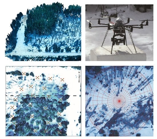
The UAV platform, the MicroKopter ARF-Okto XL (HiSystems GmbH, Moormerland, Germany, Figure 2a), was used for imagery acquisition of snow depth distribution and LAI retrieval. This octocopter is suitable for performing photogrammetric flights over limited areas (<1.5 km2). It was equipped with a commercial RGB camera: the Panasonic Lumix DMX-GX7 featuring a 16 MP Micro Four Thirds (17.3 × 13 mm) CMOS sensor fitted with a Panasonic 20 mm f/1.7 prime lens. To achieve a very high spatial resolution of centimeter-scale ground sampling distance (GSD), the flight altitude varied between 46 and approximately 73 m. Images were taken each second, with a 400 ISO speed range. The manual focus was set to infinity, to avoid focusing on single, undesired objects. All images were captured in the VIS (400–700 nm) part of the electromagnetic spectrum.
We programmed the flight path with waypoints for taking autonomous images including flight height and flight time. It was set in the corresponding MikroKopter flight planning tablet tool (MK-TT) and transferred to the copter. The typical flight duration was around 20 min in the summertime, while in the wintertime with temperatures below −10 °C, the flights were much shorter due to the rapid drain of the Lithium Polymer (LiPO) batteries. To achieve seamless coverage of the study sites, and to get a sufficient number of point pairs in the imagery, the front and side lap were both set to 80%. Before a survey flight, well distributed, predefined ground control points (GCPs) were placed over the study sites to secure accurate georeferencing of the imagery (Figure 2b,c). Some of the GCPs served as checkpoints (CPs) to assess the accuracy of the model. Permanent GCPs were marked with fixed wooden sticks to secure the same collection of GCPs during snow cover, but most of them disappeared. The remaining rods served then as permanent markers and were completed by temporary GCPs, either bullseyes or colored pink crosses, sprayed over the snow cover (Figure 2b).
For accurate positioning of GCPs and additional snow depth samples, the Global Navigation Satellite System (GNSS) Topcon HiPer SR was used in Real Time Kinematics (RTK) mode. This device measures the coordinates of the center of the GCPs with a horizontal precision of 0.01 m to 0.03 m and vertical of 0.02 m to 0.05 m at each point. To keep this level of accuracy, for each GCP and CP measurement the online RTK corrections were used as recommended by the Czech State Administration of Land Surveying and Cadastre Authority. For RTK corrections, a Virtual Reference Station (VRS) was used, which was located 5 km from the area of interest. The VRS is calculated based on real reference stations among the national permanent GNSS reference stations. Detailed technical specifications of both UAV and the camera system are included in Table 1.
2.3. Photogrammetric Processing
Before processing the images, manual pre-selection was done to remove blurred photos. All suitable images were then processed using Agisoft PhotoScan Pro (version 1.2.6) [48] to reconstruct snow-free and snow-covered DSMs, together with maps of snow depth distribution and orthomosaics from both study sites. PhotoScan is commercial software that enables full control over the all steps of photogrammetric processing, ranging from image alignment and sparse- and dense-point cloud generation, to the building of the DSM and orthoimagery [49,50]. During the processing in Agisoft PhotoScan Pro, the imagery was aligned choosing “accuracy-medium”, key point limit 40,000 and tie point limit 20,000. The point clouds were generated by using the settings “quality-medium” and “depth filtering—moderate”. After the initial image alignment process and removing evident outliers, the sparse clouds were manually georeferenced by identifying the GCP in the matched pictures and assigning them the coordinates from the GNSS post-processing (S-JTSK Krovak East North (EPSG 5514)). The checked markers which were GCPs were applied for the optimization procedure, whereas the chosen unmarked markers, in our case the CPs, served as control points to quantify the accuracy of the results and thus the total RMSE. For the absolute orientation, eight selected GCPs for the snow-free campaign were used, while six GCPs served as CPs to evaluate the accuracy of the alignments at the open site (Figure 5a). Nine GCPs were distributed with six GCPs acting as CPs for the snow-covered DSM processing at the open site (Figure 5b). Five GCPs were used for the snow-free image campaigns with four CPs in the forest zone (Figure 6a). For the other two campaigns of snow-covered imagery, four to five GCPs with four to five CPs were derived (Figure 6a,b). For the dense cloud reconstruction process “medium reconstruction quality” in Agisoft PhotoScan Pro was used to balance the computational costs with the required level of detail. The raw point clouds were exported, with a spatial resolution of 0.10 m, to perform further point cloud editing and classification in CloudCompare software [51]. Ground points were extracted from the point cloud by removing trees based on the Cloth Simulation Filter (CSF) [52]. To remove light to hard shadows on snow-covered point clouds, we used a k-means clustering algorithm after [53]. This algorithm classified the point clouds based on their RGB attributes with a Nearest Distance type classifier. The clusters were created on a training subset and then applied for the whole dataset. After classification, segmentation, and shadow removal, DSMs of 0.10 m resolution were built in GIS software [54]. Co-georeferencing were applied to georeferencing both snow and bare soil DSMs based on common GCPs used for both snow-free and snow-covered DSMs [41].
2.4. Snow Depth Data Acquisition and Analysis
For each of the studied areas, during snow-free and snow-covered period GCPs were measured. During winter manual point measurements of snow depth (HGCP) were sampled precisely above the measured GCP positions so that the x, y and z positions of the GCPs and the positions of the corresponding snow probes could be measured simultaneously. Additional arranged snow depth samples (HT) were taken at both sites to improve the overall accuracy of the generated surveys. These HT values were estimated from the means of five individual snow depth measurements taken in a 1m radius. A total of 105 HT samples in a plot of 170 × 125 m at the open site and 36 HT samples in a rectangle plot of 50 × 50 m at the forested zone were collected for each measurement survey. The idea was to cross-check the results of these two data sets against each other to ascertain if an increased quantity of ground measurements would significantly impact the overall precision of the survey when comparing them with the estimated (HUAV) snow depths. Additionally, to reduce the total error by obtaining the average of several snow depth readings at the point of observation. It must be noted here that the additional HT samples at the forest site are conducted every year due to long-term snow-cover monitoring [4,55,56]. Therefore, the study area at the forest zone was only partly covered by snow depth probing. These samples, however, were enough for the quality check, and they were also used during snow accumulation and snow ablation for the computational interpolation of manual snow depth estimates with the winter LAI obtained by the three methods. We used both datasets of manual snow depth measurement (HGCP and HT), one with more and one with fewer ground measurement reference points, to implement a preliminary evaluation of UAV performance in retrieving point values of snow depth from the DSMs of difference (DoD).
2.5. LAI Assessment
LAI measurements (Figure 3) were performed respectively at the 3 and 24 March 2017. To test the reliability of the UAV-based LAI flyovers, additional ground-based measurements using the Li-Cor LAI-2200 plant canopy analyzer (Li-COR Inc., Lincoln, USA) [57] and DHP, were conducted. During the first campaign, a little snow was still present at a few tree crowns. Additionally, dead lying wood on the ground was already snow-free. These optical methods are for indirect field measurements of LAI, producing the so-called effective LAI index (LAIeff; [58]). The optical detector of the LAI-2200 sensor is composed of five different detectors in concentric rings, each of which views a portion of the hemisphere, such as 0–13° (1st ring), 16–28° (2nd ring), 32–43° (3rd ring) and 61–74° (4th ring) [59]. This allows for the computation of radiation transmission caused by the canopy in the blue part of the spectrum and therefore calculates the LAI by comparing differential light measurements above and below the canopy [60]. Above measures served as a reference and were taken before each set of below-canopy sampling outside the forest. Below-canopy measurements with the LAI-2200 were made about 1 m above the ground in a grid of 50 × 50 m, at 10 m intervals, for 24 points at the forest site.
Each plot was estimated by means of four individual LAI values measured in a cross shape with ~1 m distance from the cross center, similar to the manner employed in [61]. The center point of the cross of each plot was marked with a blue cross symbol, which could be detected from the UAV platform to verify the accuracy of it. All readings were carried out in the morning. At both dates, the weather conditions varied between partly clear sky and overcast conditions. A narrower view cap of 270° was used to occlude the influences of the direct sun and the operator in the measurements [57]. Post processing was conducted with the FV2000 software (Li-COR Inc., Lincoln, NE, USA) [57]. To achieve LAIeff results closer to the true LAI, while maintaining consistency in comparison with the LAIeff produced by DHP, the fifth ring was excluded during data processing [62]. Hence, the view of the zenith angles corresponds to 58° which is approximately equal to the ring with the largest view angle of the hemispherical camera used in this study.
The camera was mounted on a tripod at a fixed height of 1 m above the ground. The lens aperture was fixed, and the exposure time was set to auto-mode. The geographic orientation and circular extent of the hemispherical image were applied in a northerly direction, which corresponds to 0°. Similar to the LAI-2200 plant canopy analyzer, the DHP computes the gap fraction through the camera with a hemispherical lens (fisheye) [63]. In total, 24 points were measured. LAI was processed using the Gap Light Analyzer (GLA) software (Cary Institute of Ecosystem Studies, New York, USA) [64,65].
The UAV surveys for LAI retrieval were performed in partly sunny to overcast conditions. Overcast conditions are more preferable to avoid shadows on the forest floor [60], which can hamper exact LAI retrieval, but images could be analyzed with adequate accuracy. The UAV-based LAIeff values were estimated from measurements that were taken at two different altitudes (at ~50 m and ~65 m) to determine whether there were observed differences in the LAIeff retrieval between the optimal height and higher ones. The downward-looking UAV images were taken from nadir position with a field of view (FOV) of 48°. To catch approximately the same positions of ground measurements, images were obtained at an interval of one second. Altogether, 24 points were measured within the Norway spruce stand and marked by a blue cross sprayed on the snow-cover, like those recorded by the other two optical methods. All LAI values measured in this study are effective values, so the clumping of the needles was not taken into account. GLA software, used for LAI assessment by DHP (Figure 4a,b), was also applied for LAI determination, based on UAV downward-looking images (Figure 4c,d). This allows for the processing of both custom fisheye lens distortions, and also of standard lens projections [64,65]. Here, instead of a polar projection, which is used for fisheye lenses, an orthographic standard projection for rectangle images was used in GLA software. GLA computes all zenith angles from 0 to 60° for its effective LAI. The manual segmentation based on classifying pixels as either canopy or snow. The environment of the GLA is shown in Figure 3, and the input parameters are listed in Table 2.
3. Results
3.1. Study Sites and Data Acquisition
At the open site, the total of 2093 images was acquired on two different dates from March (during snow ablation) to the end of April (after snowmelt). The sum of two DSMs and orthoimages of ~0.10 m spatial resolution was generated from the field surveys. The absolute accuracy of the derived DSMs (snow-free and snow-covered maps), relative to the measured surface points are summarized in Table 3.
At the forest site, featuring different health status of the forest stand, a total of 2494 images were captured in three campaigns from March (during snow accumulation and snow ablation) to the end of April (after snowmelt) with the same data acquisition parameters as at the open site. The total of three DSMs and orthoimages of ~0.10 m spatial resolution was generated and the absolute accuracy of the derived DSMs (snow-free and snow-covered) of the root mean square (RMSE) for x, y, and z together with the area total error in m of the CPs are listed Table 3.
3.2. UAV-Based Snow Depth Estimations vs. Manual Snow Depth
A total of five DSMs were generated from the winter during snow accumulation and ablation, and from the snow-free fieldwork campaigns. The hillshades computed from UAV data during snow-free and snow-covered time, along with the applied GCPs, are shown in Figure 5a,b, for the open field. For the forest zone, only the hillshades during peak accumulation and ablation are visualized (Figure 6a,b) with the corresponding GCPs. GCPs, taken during wintertime also served as reference snow depth points at the GCP positions (HGCP) and were selected in support of co-georeferencing the snow-free DSMs with the snow-covered DSMs.
The difference between the supplementary HT probes and estimated HUAV measurements are visualized as interpolated maps (Figure 5c and Figure 6c,d ), showing the spatial distribution of the snow height differences. Three DoDs were created (Figure 5d and Figure 6e,f ) based on standard photogrammetric procedure Usually, by subtracting the snow-free DSMs from the snow-covered DSMs, the snow depth values appeared negative in the maps, which were classified as outliers but not masked out, and depicted as zero values in the maps, for readability. This discrepancy has already been noted during photogrammetric surveys [27,28,40] and can be attributed to the effect of compressible vegetation and instrumental precision [28,66].
The snow height differences were ascertained as mean values within 1 m buffer to be comparable with the HT samples determined from the mean of five snow depth measurements taken in 1 m radius. White gaps of the created DSMs mark the filtered vegetation (e.g., trees and bushes) and might be due to shadows or poor matching over some area of the snow surface (any resulting couple points in the horizontal plane due to the homogeneity of snow). Kernel Interpolation was used to display the spatial distribution of the snow height differences between HT probes and estimated HUAV measurements (Figure 5c and Figure 6c,d ). The Kernel Interpolation allows the prediction of the output surface with smoother barriers [67] and uses the shortest distance between points so that points on the sides of the specified nontransparent (absolute) barrier are connected by a series of straight lines. It is advantageous because it leaves the parts out which are not snow-covered, or where trees were removed from the point cloud.
The snow height differences were ascertained as mean values within 1 m buffer to be comparable with the HT samples estimated from the mean of five snow depth measurements taken in 1 m radius (Figure 6). White gaps of the created DSMs display the filtered trees and dead lying trunks on the ground and might be due to shadows or poor matching over some area of the snow surface (any resulting couple points in the horizontal plane due to the homogeneity of snow). The snow depth validation outcomes are summarized in Table 4. Statistics include the mean bias, the correspondent SD, the mean absolute error (MAE), and the RMSE between HGCP and HUAV, as well as HT and HUAV. Mean bias quantifies the mean magnitude of the over- (positive values) or under- (negative values) prediction of the DSM concerning manual snow depth measurements. The SD quantifies the variability of the error. Both MAE and RMSE determine the accuracy between the manual snow depth observations (HGCP and HT) and the estimated UAV-based snow depth values extracted from the DoDs in relevant to HGCP points and HT area. The results indicate an overall average performance for all the surveyed areas, with results agreeing with relevant literature. For instance, [37] reached an accuracy of the DSMs relative to the measured variable surface points due to dynamic conditions with varying RMSE from 0.04 m to 0.19 m with few problematic flights showed larger RMSE of up to 0.32 m [38] estimated snow depth distribution with an RMSE of 0.30 m. Better results below 0.30 m were predicted by [41] with RMSE between 0.05 m and 0.18 m.
One-to-one (1:1) comparisons between all snow depth measurements (HGCP and HT) and estimated HUAV snow values are provided in Figure 7a,b. The error does not change sufficiently with the snow depth (Figure 7a), showing a moderate overall correlation by all values taken at GCP positions, whereas the overall correlation coefficient is considerably weaker when comparing HT measurements with HUAV estimated snow depth values (Figure 7b). Most of the HUAV snow depth values are underestimated, especially in the open area (Figure 7b). The similar slope of regression line both in Figure 7a,b suggest the relative good robustness of result when using fewer measurement points. However, the much more significant variance in Figure 7b shows that only 10 GCPs cannot capture the variability of snow depth in such complex terrain (many small depressions and elevations due to windthrow, hampered the results). The decision to use a denser grid of arranged ground measurements increased the spatial coverage, snow depth variability and therefore much more confident. In addition to the above consideration, we extracted snow depth profiles of the estimated HUAV measurements from the DoDs (Figure 5d and Figure 6e,f ) and plotted them along with the manual taken HT snow depths (Figure 5c and Figure 6c,d ). Figure 8 shows the produced transects in respectively West-East and North-South directions (four profiles for each snow event in total) during snow ablation at the open site and snow accumulation and ablation at the forest site.
Comparison of the estimated HUAV snow depth and manual probing HT in Figure 8 reveals that the HUAV measurements run a relatively similar course like manual probing but by nearly two orders of magnitude lower, especially in the case of the open area (Figure 8a–d). Systematically superposition of manual probe locations is observed compared to the lower corresponded run of the estimated HUAV snow depth profile (Figure 8a–d). Except one HUAV point is higher than HT as shown in Figure 8a due to different underlying vegetation structure. The forest transects (Figure 8e–h) show more variability between the HUAV snow depths and HT data along the profiles. These transects show partly the HUAV snow depths reproducing all of the features revealed by the manual probes, despite the several confounding effects (e.g., tree canopy, tree stumps, and dead lying wood on the ground or changing vegetation structure). In few locations along the profiles, the HUAV values indicate changes up to 0.5 m lower than revealed by the probes within the healthy forest part (e.g., Figure 8e) during both snow conditions displaying zero distributions. Higher appearing HUAV values than HT can be explained by snow-covered wood features, such as lying dead trunks or dead wood on the ground or due to different underlying vegetation structure, especially at the forest site (Figure 8a,e,f,g,h).
3.3. Optical Indirect Estimation of LAIeff
By taking LAI-2200 canopy analyzer and DHP as benchmarks, the correlations between the measured values of the UAV-based LAIeff and the reference values were calculated and plotted in Figure 9a,b. 1:1 relationship across these methods were significant in a few instances. A high relationship was obtained between the two reference methods DHP and LAI-2200 (Figure 9a). The correlations between the UAV-based LAIeff data and LAI-2200 were less strong (Figure 9a). The correlations between UAV-based LAIeff observations and DHP were as good as between both reference methods (Figure 9b). Most of the observed values were all distributed above the 1:1 line (Figure 9a,b). The observed LAI values using UAV and DHP methods were underestimated (Figure 8a). A similar 1:1 relationship was shown in the scatter plot in Figure 9b. The observed UAV values were almost all above the 1:1 line except some values between 0 and 3. In both cases, the observations provided overestimations. RMSE indicates the accuracy of all utilized methods; Figure 9a shows the UAV-based LAI estimation has a lower accuracy comparing to the observed DHP values with LAI-2200 observations. On the contrary, Figure 9b shows a higher accuracy by comparing the UAV and DHP methods.
3.4. Relationship between Indirect Winter LAIeff and Snow Depth
To provide better visualization of the HT measurements and LAIeff values taken by the different sampling methods, these data points were also interpolated using Kernel Interpolation. All data presented in Figure 10a,b were considered for data interpolation. However, only the overlapping data points within the figures were valid. The interpolated HT values during both snow conditions are shown in Figure 10c,d, whereas the interpolated LAI data are presented in Figure 10e,f. During snow accumulation, HT ranged between 0.38 m and 0.99 m (Figure 10c), while during snow ablation the HT measurements varied between 0.19 m and 0.68 m (Figure 10d). In both cases, higher snow depth values appeared in the upper part of the study plot where the forest was mostly damaged, and less vegetation canopy was existent. On the contrary, the lower part, which mainly consisted of healthy trees, was below the tree canopy and therefore, lower snow depth was present. This trend goes hand-in-hand with the ground-measured LAI and UAV-based LAI estimates that show an opposite pattern (Figure 10e–j). The higher the LAI values, the lower the snow depth, and vice versa. The apparent north-south trend how visible in Figure 10c–j is not affected by the applied interpolation technique, but it reflects the captured data in the field and thus makes it clear how canopy structure plays a primary control on snow depth.
The LAI-2200 plant canopy analyzer measured the highest LAI values, with maximum LAI estimates of 5.34 in the denser part of the forest, while the UAV-based LAI measurements showed the lowest maximum values of 3.27 and 3.30, taken at 50 m and 65 m, respectively. Overall, all methods showed the same pattern of LAI estimates (Figure 10e–j), with higher LAI values indicating lower snow depth. It is well accepted that snow storages in the coniferous forest characterized by high LAI values are lower compared to open environments, or as in this case, damaged portions, because of the processes of interception, sublimation, evaporation and wind redistribution [5,10,15,67]. Consequently, there is also a statistically significant correlation between LAIeff and manual HT, particularly during snow accumulation (Figure 11a). Considering that the relationship was developed from ground-measurements and by UAV at two different altitudes, the fit is entirely fair (Figure 11a). The R2 between HT and the LAI-2200 plant canopy analyzer was the highest during snow accumulation (Figure 11a). LAIeff-UAV (50 m) and DHP showed similar correspondence. The lowest relationship was between LAIeff-UAV (65 m) and the LAI-2200 plant canopy analyzer. The influence of winter LAI can be seen in its control of the snow depth within the different forest stands during snow accumulation and ablation. LAIeff-UAV (50 m) and DHP presented the best fit during snowmelt, whereas LAIeff-2200 and LAIeff-UAV (65 m) exhibited an instead scattered relationship (Figure 11b).
4. Discussion
4.1. Snow Depth Validation of Open vs. Forest Site
Snow depth variabilities were captured over the meadow and complex underlying topography in the forest. High snow accumulation zones were linked with topographical depressions, especially at the open area, whereas only some parts were linked more efficiently at the forest site during both snow events. However, as with any remote sensing technique, errors can exist at any stage of image acquisition or analysis. The comparison between measured and estimated snow depth for the HGCPs probes ranged between 0.08 m for the open area through 0.15 m during spring snow accumulation in the forest and 0.09 m during spring snow ablation within the forest stand. The snow depth estimates compared between a denser network of snow probes varied between 0.16 m for the open field through 0.32 m during snow accumulation to 0.31 m during snow ablation for the HT measurements at the forest site. With an increasing number of sample points, the results deteriorated, especially at the forest site. Notably, it makes a difference between randomly selected fewer snow probes (HGCP) taken within canopy gaps or near the canopy edges than a denser network of snow probes (HT) taken as well under canopy positions. In the forest a denser network of snow probes is more sensible to sources in the context of uncertainty, it highlights the complexity of the terrain and vegetation-induced variability in snow properties. However, the results confirmed that the overall robustness of our model capturing snow depth variabilities over more sample points does not differ much at the open site. A similar finding is supported by [18] that a higher number of manual snow probes do not necessarily affect the overall precision of the survey regarding the RMSE as well.
Likewise, the accuracy of the precision didn’t improve by taking more ground samples in this case. However, these statistics are based on a more limited validation power (point-scale measurements) than using other methods, e.g., Airborne laser scanning (ALS). ALS is capable of accurately mapping snow depth for small to large aerial extents, and at high spatial resolution accuracy of snow depth estimates of 0.15 m as reported by [22]. Additionally, using terrestrial laser scanning (TLS) might be more efficient to improve ground mapping in the forest environment. Data acquisition with TLS is time and manpower consuming, and only possible at easily accessible spots [38]. This study proves that snow depth statistics are consistent with previous studies [18,41,64,68,69,70,71]. It also confirms that the UAV application can reach high-quality snow depth estimates in different environments and vegetation, although lower errors were expected at the open area compared to the forest site.
Apparently, ground properties play a crucial role in the precise creation of accurate DSMs [5]. In case of the open field, meadow coverage (tall grass) at the base of the snow cover and scattered boulders had a strong influence on the results. There is a source of systematic error between HGCP and HUAV that can be assigned to the effect of vegetation, in particular to the grass cover. The height of the dense montane grass cover, which is in the study area dominated by Carex Rostrata and Nardus stricta L. [72], can reach up to 20–30 cm in the summer (Figure 12a). The grassland creates compact formations, covering the forest-free areas, where the optical imagery cannot reach the ground, which results in a corresponding shift of surface elevation. In winter, the grass is pressed down to the ground by the snow cover (Figure 12b), forming a snow-free layer of one centimeter below the snowpack. In the areas affected by forest disturbance, the lying trunks of dead trees and branches, the detection of the ground make a compact layer, which can result in an artificial shift of between the values, determined by geodetical surveying and the photogrammetric reconstruction. We assume that the snow-free DSM ground elevation is higher than the snow-covered DSM, causing the underestimation of HUAV results, and overestimation of HGCP and HT, as previously reported by [36,38,73]. This is also visible by the produced transects. Interpretation of the difference in snow depth profiles between the estimated HUAV measurements and manual probing HT is complicated especially in the forest zone by the fact that photogrammetric techniques do not work accurately above and below tree canopies resulting in zero snow depth values. Thus, extra care in interpretation needs to be taken in forests. Profiles of estimated HUAV along the open area showed better correspondence with manual probing. This might be explained by the relatively homogenous terrain of a wide shallow slope characterized by meadow coverage. However, despite the lower or higher shifts of the estimated HUAV measurements, we tried to minimize it by appropriate scheduling of the imaging campaign. The open field status was captured in early spring, just after the snowmelt (30 April 2017), before the start of the new vegetation season. The same applies to the forest site, which the dead wood on the ground could potentially cause error mapping during snow-free period and winter (Figure 12c,d), and also by difficulties applying UAV images above, below, and around trees, resulting in more significant gaps in the DSMs. Where available, the use of aerial LiDAR data as a reference dataset can significantly reduce this source of uncertainty and help to get a more accurate representation of the ground surface.
Vegetation effects are not the only issue. As the number of ground-based snow depth measurements is small, these data represent only a reduced variability concerning the complete range of variation of UAV-based snow depth evaluation. When estimating the snow depth for each pixel, the overall error derives from the two generated DSMs used for the subtraction. The error source on an SfM made DSM is divided into two categories: the photogrammetric reconstruction error; and, the georeferencing error. The photogrammetric error depends on the overall quality of the dataset, while the GNSS or post-processing quality cause the georeferencing error, the GCPs manual identification in the image, and the GNSS accuracy height point measurements [41]. This, in turn, depends on the quality of the sparse point cloud and, therefore, the quality of the methodology with which the images were acquired at the end [5]. For the future, an even better qualitative assessment of the snow-covered surface can be reached by applying the combined mapping of VIS and near-infrared (NIR) images, as has been done by [5,38]. Furthermore, a promising HUAV approach might be to capture not only UAV images in the nadir position, but to combine them with oblique photos, taken by the same platform. The oblique imagery would enable minimizing the ground coverage by the tree crowns for the forest locations and to get more complex coverage of the ground. As the photogrammetric software, based on SfM technique allows a combination of the nadir and oblique imagery, such an approach could provide a better description of the ground surface below the tree stamps.
4.2. Validation of the Winter LAI
The assessment of the effect of different forest structures, forest disturbances, and open sites, on snow accumulation and snowmelt, is often done using modelling approaches (e.g., hydrological models, snowpack models, and land surface schemes of climate models) and collecting field data [8,39] based on measured or simulated field data. This means that these conceptualizations need input parameters to model real physical processes. Depending on the model, different predictors can be used to explain the variability of snow accumulation and ablation in distinct areas, as was done by [4]. They used the following predictors, i.e., elevation, slope, slope orientation, LAI, canopy openness, amount of shortwave radiation, irradiance, mean daily irradiance, snow depth, air temperature, and the date of sampling. To collect all these data is time intensive. Why shouldn’t it be used for the estimation of LAIeff, based on downward-looking images, where snow background is used instead of the sky fraction since UAV digital photogrammetry is a reliable tool to measure snow depth? Substituting this two-in-one approach for the heretofore standard methods helps resolve many of the aforementioned problems, although additional test data is still required to provide a reference standard.
Although the LAI estimates tested using UAV produced, overall, sufficient LAIeff values, even at different altitudes compared to the other devices, i.e., the LAI-2200 plant canopy analyzer, and DHP, small discrepancies between these methods appeared. Indeed, there was constant underestimation of the UAV-based LAI compared with the reference data. That might be the fact that snow was still present at few tree crowns during snow accumulation that caused these underestimations, even though the correspondence during snow ablation between UAV-based LAIeff and LAIeff LiCor-2200 or DHPeff were slightly better due to the snow uncovered wood on the ground causing higher LAIeff values. It has also been approved that there is an overestimation of the LAIeff performed by LAI-2200 plant canopy analyzer compared to the other method results [44]. Here, a cap of 270° was used to hide both the sun and the operator from the sensor’s view and reduce the required clearing size for above-canopy readings in a denser forest. This cap is also preferable if the goal is to measure LAIeff [57]. Nonetheless, a narrower view cap of 90° would probably be more appropriate, due to the diverse vegetation structure and the dynamic changes in spruce forest LAI in the study plot. Likewise, the LAIeff values obtained by DHP present slightly overestimated than the LAIeff UAV estimated.
It is essential, therefore, to know from which altitude the LAI value should be taken, to compare with the ground measurements [61]. It was assumed that the optimal flight altitude for LAIeff UAV estimates would be around 50 m. The difference in the results could have been caused by a different shooting zenith angle or camera zenith angle since the DHP and UAV methods had nearly similar software configurations, and, except for the different backgrounds, almost identical sampling methods in the experiment [74]. LAI extraction might be affected by the shooting angle regarding the proportion of leaf elements that might be influenced by the shooting angle of the different FOV of the cameras. To detect the same area with a smaller viewing angle (48°) on the UAV mounted camera, the observation height should be about tan (74°)/(48°) = 1.5 times the tree height, which varied in the test plot from 15 m to 20 m, with an average value of 17.5 m. Thus, the optimal flight altitude would be ~26 m. However, the tested flight heights at 50 m and 65 m show differences in capturing LAI (Figure 13). As the research area was covered by healthy and bark-beetle damaged trees, the LAI values were not kept at a very stable level. Variations in LAIeff values appear mainly due to the heterogeneous structure of the forest. In the future, additional NIR or oblique imagery could be applied to improve the assessment quality of the DSM for snow depth mapping, as well as the LAI retrieval.
Moreover, in the case of UAV-based LAI estimates, the calculated LAI values might depend on the amount of snow cover because it also accounts the interception of snow-free dead lying branches and trees on the ground during snow ablation that the other methods are not taking into consideration. The ideal condition to perform UAV-based LAI retrieval is to have more snow on the ground because there will be fewer objects such as dead lying branches and trees interfere with the images, which could potentially affect the calculation of the LAIeff values. However, this much is sure: that LAI decreased with increasing flight altitude during both snow accumulation and snowmelt, as observed in Figure 13 a,b. The lower the altitude is, the smaller is the area seen by the camera and the more significant is the variety of different scenes, whereas higher flights produce more averaged LAI values [61]. A similar trend was observed by [45,61,75].
4.3. Validation between Snow Depth and LAI
As expected, LAIeff values negatively correlated to HT data appeared at the investigated forest site more often during snow accumulation than during ablation (Figure 11). That was predicted by all methods used here. The lower the HT measurements were, but the higher the LAI values, and vice versa. In general, increased LAI values mean more leaves in reality, leading to more surface covered by the canopy rather than by snow cover [44]. So, the presence of trees alters the processes that shape, in particular, snow cover accumulation. As a consequence, the amount of forest canopy, often described by estimates of LAI, are inversely related to snow accumulation [74]. However, a considerable variability between LAIeff values and HT were observed in measured comparisons between forest snow ablation and forest accumulation.
It is proven that the forest canopy interacts directly and indirectly with snow, and therefore impacts in significant ways on snow cover, especially during snowmelt periods [43]. The most direct is snow interception (e.g., canopy structure). Intercepted snow can be stored in the canopy, sublimated directly to the atmosphere when it is getting warmer [45,75], or change phase before reaching the underlying snow cover [76,77]. Since the investigated forest site consists of a paired forest and clearing structure, snow accumulates and melts differently. During snow accumulation, the clearing part contained the immense quantity of snow, where the LAI values were low. Whereas in the adjacent dense, healthy forest, less snow accumulated, due to increased interception and an increase in longwave radiation.
With respect to snow melting, snow should last longer in the clearing part than in the denser forest. Concerning the low correlation between snow depth and LAI during snow ablation, and the tendency of some outliers showing a slight correlation of higher LAI values with higher snow depth. The reason for that might be that some of the intercepted snow sluffed off the canopy, particularly in areas of denser forest due to the higher LAI values, and was added to beneath-forest accumulation [12]. In fact, this assumption should be treated with care. It is clear that the snow variability cannot be determined via two parameters only, e.g., snow depth and LAI. There are more processes influencing snow distributions including the amount of shortwave radiation, air temperature, partial snowmelt periods, meltwater dripping from the canopy, wind sheltering, and snow redistribution due to the wind, elevation, slope orientation, and slope angle. Although the latter may not be relevant to a small forest area studied here, since it is a flat area, it might be suitable for open sites. The existing forest heterogeneity makes it difficult to postulate a clear direction of interpretation. It can be concluded that the use of LAI as a prediction parameter serves better for snow accumulation events than for snowmelt because it better describes snow interception. Hence, for snowmelt, factors that are more closely related to radiation and topography could give better results when describing the snow depth variability at a plot scale. Nevertheless, the substantial differences in spatial resolutions between manual and UAV-based snow depth measurements (meter vs. centimeters) are that small scale differences in both snow depth and vegetation structure cannot be captured by manual measurements either snow depth using probe or DHP. Therefore, to add more locations with manual measurements and consequent interpolation cannot bring the same level of detail associated with UAV which measures in cm resolution.
5. Conclusions
This study has presented the potential of small footprint UAV data for deriving metrics such as snow depth (snow metric) and LAI (forest metric) using single flights. As was found in previous studies, we could show that it is possible to estimate snow depth and indirect LAI from UAV data by using RGB-based UAV imagery. Snow depth was computed by subtracting snow-free from snow-covered DSMs during different snow conditions and compared to fewer and with more manual ground measurements. Differences in measured values obtained by these snow samplings strategies draw distinctions. Effective winter LAI estimates conducted as well from downward-looking UAV images were compared to conventional optical methods (e.g., DHP and LAI-2200 canopy analyzer) producing reasonable but underestimated LAIeff values. With increased flight height of the UAV, lower estimated LAI values were determined for all forest structures.
The relation between LAI and snow depth was analyzed for different snow conditions. As expected, LAIeff values negatively correlated to snow depth data during both snow conditions at the forest site. For snowmelt, the LAI as one of the predictors for snow distribution in forested areas represented weaker correlations. The reason is most likely that LAI is a much stronger predictor for snow accumulation, because it better describes the snow depth distribution during the accumulation period, while for snowmelt, more processes influence the snow variability. Elevation and topography have a marginal effect here, as the study plot in the forest zone is situated in a flat area. Thus, for snowmelt, factors that are more closely related to radiation and topography might give better results when describing the snow depth variability at a smaller scale.
To this end, the results demonstrated that, with this combined method, snow depth and LAI retrieval could be recorded simultaneously with one UAV survey. The conjoint survey can significantly improve the efficiency of both aerial and field mapping of snow cover distribution in areas featuring variable structure and health status of the forest canopy. In such areas, it proved reliability in the determination of the snow depth variation along with the LAI, enabling the interpretation of the effects of canopy coverage on snow accumulation and ablation.
However, the largest advantage of the UAV technology here is the high resolution and the high level of detail regarding the snow-covered terrain and the quick monitoring of indirect LAI compared to simple manual measurements of snow depth and point measurements of DHP or using LiCor-2200. By improving this method both parameters snow depth and indirect LAI might be used as input parameters for snow models captured in reduced time.
Further work is required to examine the performance of snow depth change mapping in terms of the precision of snow depth change estimates under denser canopies where the non-vegetated surface is mainly covered and the use of infrared photography improves identification of different snow features such as windblown snow into openings in the forest, ice crusts, and wet snow surfaces. Attributes that need improvement as they affected the thresholding of binary images for the indirect LAI analysis were shadows and snow on tree crowns.
Author Contributions
T.L. designed the study, performed the UAV-based data acquisition, data processing, analyzes and wrote the substantial parts of the manuscript. J.L. supervised the study and contributed to methodology, data analysis and discussion parts. M.J. assisted in the field (performing manual snow depth probing) and contributed to the discussion part. The manuscript has been prepared with the contribution of all co-authors.
Funding
The research was supported by the EU COST Action 1306 project LD15130 “Impact of landscape disturbance on the stream and basin connectivity” and by the Czech Science Foundation project 19-05011S. The authors would like to thank Robert Minarik, for help in designing the UAV flight plan and for collecting ground control points (GCPs) in the field.
Conflicts of Interest
Authors declare no conflict of interest.
References
- Wang, D.; Hollaus, M.; Puttonen, E.; Pfeifer, N. Automatic and self-adaptive stem reconstruction in landslide-affected forests. Remote Sens. 2016, 8, 974. [Google Scholar] [CrossRef]
- Dong, C. Remote sensing, hydrological modeling and in situ observations in snow cover research: A review. J. Hydrol. 2018, 561, 573–583. [Google Scholar] [CrossRef]
- Dong, C.; Menzel, L. Snow process monitoring in montane forests with time-lapse photography. Hydrol. Process. 2017, 31, 2872–2886. [Google Scholar] [CrossRef]
- Jenicek, M.; Pevna, H.; Matejka, O. Canopy structure and topography effects on snow distribution at a catchment scale: Application of multivariate approaches. J. Hydrol. Hydromech. 2018, 66. [Google Scholar] [CrossRef]
- Pomeroy, J.W.; Gray, D.M.; Hedstrom, N.R.; Janowicz, J.R. Physically based estimation of seasonal snow accumulation in the boreal forest. In Proceedings of the 59th eastern snow conference, Stowe, VT, USA, 5–7 June 2002; pp. 93–108. [Google Scholar] [CrossRef]
- Ellis, C.R.; Pomeroy, J.W.; Essery, R.L.H.; Link, T.E. Effects of needleleaf forest cover on radiation and snowmelt dynamics in the Canadian Rocky Mountains. Can. J. For. Res. 2011, 41, 608–620. [Google Scholar] [CrossRef]
- Melloh, R.A.; Hardy, J.P.; Davis, R.E.; Robinson, P.B. Spectral albedo/reflectance of littered forest snow during the melt season. Hydrol. Process. 2001, 15, 3409–3422. [Google Scholar] [CrossRef]
- Elder, K.; Dozier, J.; Michaelsen, J. Snow accumulation and distribution in an Alpine Watershed. Water Resour. Res. 1991. [Google Scholar] [CrossRef]
- Strasser, U.; Warscher, M.; Liston, G.E. Modeling Snow–Canopy Processes on an Idealized Mountain. J. Hydrometeorol. 2011, 12, 663–677. [Google Scholar] [CrossRef]
- Garvelmann, J.; Pohl, S.; Weiler, M. From observation to the quantification of snow processes with a time-lapse camera network. Hydrol. Earth Syst. Sci. 2013, 17, 1415–1429. [Google Scholar] [CrossRef] [Green Version]
- Moeser, D.; Roubinek, J.; Schleppi, P.; Morsdorf, F.; Jonas, T. Canopy closure, LAI and radiation transfer from airborne LiDAR synthetic images. Agric. For. Meteorol. 2014, 197, 158–168. [Google Scholar] [CrossRef]
- Lundquist, J.D.; Dickerson-Lange, S.E.; Lutz, J.A.; Cristea, N.C. Lower forest density enhances snow retention in regions with warmer winters: A global framework developed from plot-scale observations and modeling: Forests and Snow Retention. Water Resour. Res. 2013, 49, 6356–6370. [Google Scholar] [CrossRef]
- Revuelto, J.; López-Moreno, J.-I.; Azorin-Molina, C.; Alonso-González, E.; Sanmiguel-Vallelado, A. Small-Scale Effect of Pine Stand Pruning on Snowpack Distribution in the Pyrenees Observed with a Terrestrial Laser Scanner. Forests 2016, 7, 166. [Google Scholar] [CrossRef]
- Stähli, M.; Gustafsson, D. Long-term investigations of the snow cover in a subalpine semi-forested catchment. Hydrol. Process. 2006, 20, 411–428. [Google Scholar] [CrossRef]
- Stähli, M.; Jonas, T.; Gustafsson, D. The role of snow interception in winter-time radiation processes of a coniferous sub-alpine forest. Hydrol. Process. 2009, 23, 2498–2512. [Google Scholar] [CrossRef]
- Varhola, A.; Coops, N.C.; Weiler, M.; Moore, R.D. Forest canopy effects on snow accumulation and ablation: An integrative review of empirical results. J. Hydrol. 2010, 392, 219–233. [Google Scholar] [CrossRef]
- Essery, R.; Morin, S.; Lejeune, Y.; B Ménard, C. A comparison of 1701 snow models using observations from an alpine site. Adv. Water Resour. 2013, 55, 131–148. [Google Scholar] [CrossRef]
- Avanzi, F.; Bianchi, A.; Cina, A.; De Michele, C.; Maschio, P.; Pagliari, D.; Passoni, D.; Pinto, L.; Piras, M.; Rossi, L. Centimetric Accuracy in Snow Depth Using Unmanned Aerial System Photogrammetry and a MultiStation. Remote Sens. 2018, 10, 765. [Google Scholar] [CrossRef]
- Jin, S.; Qian, X.; Kutoglu, H. Snow Depth Variations Estimated from GPS-Reflectometry: A Case Study in Alaska from L2P SNR Data. Remote Sens. 2016, 8, 63. [Google Scholar] [CrossRef]
- Larson, K.M. GPS interferometric reflectometry: Applications to surface soil moisture, snow depth, and vegetation water content in the western United States: GPS interferometric reflectometry. Wiley Interdiscip. Rev. Water 2016, 3, 775–787. [Google Scholar] [CrossRef]
- McCreight, J.L.; Small, E.E.; Larson, K.M. Snow depth, density, and SWE estimates derived from GPS reflection data: Validation in the western US. Water Resour. Res. 2014, 50, 6892–6909. [Google Scholar] [CrossRef]
- Deems, J.S.; Painter, T.H.; Finnegan, D.C. Lidar measurement of snow depth: A review. J. Glaciol. 2013, 59, 467–479. [Google Scholar] [CrossRef]
- Grünewald, T.; Lehning, M. Are flat-field snow depth measurements representative? A comparison of selected index sites with areal snow depth measurements at the small catchment scale: Representativeness of flat field snow depth measurements. Hydrol. Process. 2015, 29, 1717–1728. [Google Scholar] [CrossRef]
- Grünewald, T.; Schirmer, M.; Mott, R.; Lehning, M. Spatial and temporal variability of snow depth and ablation rates in a small mountain catchment. Cryosphere 2010, 4, 215–225. [Google Scholar] [CrossRef] [Green Version]
- Jaakkola, A.; Hyyppa, J.; Puttonen, E. Measurement of Snow Depth Using a Low-Cost Mobile Laser Scanner. IEEE Geosci. Remote Sens. Lett. 2014, 11, 587–591. [Google Scholar] [CrossRef]
- Grünewald, T.; Stötter, J.; Pomeroy, J.W.; Dadic, R.; Moreno Baños, I.; Marturià, J.; Spross, M.; Hopkinson, C.; Burlando, P.; Lehning, M. Statistical modelling of the snow depth distribution in open alpine terrain. Hydrol. Earth Syst. Sci. 2013, 17, 3005–3021. [Google Scholar] [CrossRef] [Green Version]
- Bühler, Y.; Marty, M.; Egli, L.; Veitinger, J.; Jonas, T.; Thee, P.; Ginzler, C. Snow depth mapping in high-alpine catchments using digital photogrammetry. Cryosphere 2015, 9, 229–243. [Google Scholar] [CrossRef] [Green Version]
- Nolan, M.; Larsen, C.; Sturm, M. Mapping snow-depth from manned-aircraft on landscape scales at centimeter resolution using Structure-from-Motion photogrammetry. Cryosphere Discuss. 2015, 9, 333–381. [Google Scholar] [CrossRef]
- Prokop, A.; Schirmer, M.; Rub, M.; Lehning, M.; Stocker, M. A comparison of measurement methods: Terrestrial laser scanning, tachymetry and snow probing for the determination of the spatial snow-depth distribution on slopes. Ann. Glaciol. 2008, 49, 210–216. [Google Scholar] [CrossRef]
- Machguth, H.; Eisen, O.; Paul, F.; Hoelzle, M. Strong spatial variability of snow accumulation observed with helicopter-borne GPR on two adjacent Alpine glaciers. Geophys. Res. Lett. 2006, 33. [Google Scholar] [CrossRef] [Green Version]
- Farinotti, D.; Magnusson, J.; Huss, M.; Bauder, A. Snow accumulation distribution inferred from time-lapse photography and simple modelling. Hydrol. Process. 2010, 24, 2045–2201. [Google Scholar] [CrossRef]
- Parajka, J.; Haas, P.; Kirnbauer, R.; Jansa, J.; Blöschl, G. Potential of time-lapse photography of snow for hydrological purposes at the small catchment scale: Potential of time-lapse photography of snow for hydrological purposes. Hydrol. Process. 2012, 26, 3327–3337. [Google Scholar] [CrossRef]
- Dietz, A.J.; Kuenzer, C.; Gessner, U.; Dech, S. Remote sensing of snow—A review of available methods. Int. J. Remote Sens. 2012, 33, 4094–4134. [Google Scholar] [CrossRef]
- Cimoli, E.; Marcer, M. Digital Elevation Model Reconstruction of a Glaciarized Basin Using Land-Based Structure from Motion. Available online: https://pdfs.semanticscholar.org/8757/eb995c9538664abb477287b473b4fac82a2c.pdf?_ga=2.114940608.653756116.1551329016-1294446320.1529472521 (accessed on 28 February 2019).
- Elder, K.; Rosenthal, W.; Davis, R.E. Estimating the spatial distribution of snow water equivalence in a montane watershed. Hydrol. Process. 1998, 12, 1793–1808. [Google Scholar] [CrossRef]
- Vander Jagt, B.J.; Durand, M.T.; Margulis, S.A.; Kim, E.J.; Molotch, N.P. On the characterization of vegetation transmissivity using LAI for application in passive microwave remote sensing of snowpack. Remote Sens. Environ. 2015, 156, 310–321. [Google Scholar] [CrossRef]
- De Michele, C.; Avanzi, F.; Passoni, D.; Barzaghi, R.; Pinto, L.; Dosso, P.; Ghezzi, A.; Gianatti, R.; Della Vedova, G. Microscale variability of snow depth using U.A.S. technology. Cryosphere 2015, 9, 1047–1075. [Google Scholar] [CrossRef]
- Bühler, Y.; Adams, M.S.; Bösch, R.; Stoffel, A. Mapping snow depth in alpine terrain with unmanned aerial systems (UAS): Potential and limitations. Cryosphere Discuss. 2016, 1–36. [Google Scholar] [CrossRef]
- Harder, P.; Schirmer, M.; Pomeroy, J.; Helgason, W. Accuracy of snow depth estimation in mountain and prairie environments by an unmanned aerial vehicle. Cryosphere 2016, 10, 2559–2571. [Google Scholar] [CrossRef] [Green Version]
- Bühler, Y.; Adams, M.S.; Stoffel, A.; Boesch, R. Photogrammetric reconstruction of homogenous snow surfaces in alpine terrain applying near-infrared UAS imagery. Int. J. Remote Sens. 2017, 38, 3135–3158. [Google Scholar] [CrossRef]
- Cimoli, E.; Marcer, M.; Vandecrux, B.; Bøggild, C.E.; Williams, G.; Simonsen, S.B. Application of Low-Cost UASs and Digital Photogrammetry for High-Resolution Snow Depth Mapping in the Arctic. Remote Sens. 2017, 9, 1144. [Google Scholar] [CrossRef]
- Metcalfe, R.A.; Buttle, J.M. A statistical model of spatially distributed snowmelt rates in a boreal forest basin. Hydrol. Process. 1998, 12, 1701–1722. [Google Scholar] [CrossRef]
- Hedstrom, N.R.; Pomeroy, J.W. Measurements and modelling of snow interception in the boreal forest. Hydrol. Process. 1998, 12, 1611–1625. [Google Scholar] [CrossRef]
- Jonckheere, I.; Fleck, S.; Nackaerts, K.; Muys, B.; Coppin, P.; Weiss, M.; Baret, F. Review of methods for in situ leaf area index determination. Agric. For. Meteorol. 2004, 121, 19–35. [Google Scholar] [CrossRef]
- Manninen, T.; Korhonen, L.; Voipio, P.; Lahtinen, P.; Stenberg, P. Airborne estimation of boreal forest LAI in winter conditions: A test using summer and winter ground truth. IEEE Trans. Geosci. Remote Sens. 2012, 50, 68–74. [Google Scholar] [CrossRef]
- Roubínek, J.; Moeser, D.; Pavlásek, J.; Jonas, T. Linking Snow Distribution and Forest Canopy Characteristics by Way of Hemi-Spherical Photography. Available online: http://arc.lib.montana.edu/snow-science/objects/ISSW13_paper_O4-26.pdf (accessed on 28 February 2019).
- Miřijovský, J.; Langhammer, J. Multitemporal Monitoring of the Morphodynamics of a Mid-Mountain Stream Using UAS Photogrammetry. Remote Sens. 2015, 7, 8586–8609. [Google Scholar] [CrossRef] [Green Version]
- Agisoft PhotoScan User Manual. Available online: http://www.agisoft.com/pdf/photoscan-pro_1_2_en.pdf (accessed on 14 March 2016).
- Verhoeven, G. Taking computer vision aloft - archaeological three-dimensional reconstructions from aerial photographs with photoscan. Archaeol. Prospect. 2011, 18, 67–73. [Google Scholar] [CrossRef]
- Koutsoudis, A.; Vidmar, B.; Ioannakis, G.; Arnaoutoglou, F.; Pavlidis, G.; Chamzas, C. Multi-image 3D reconstruction data evaluation. J. Cult. Herit. 2014, 15, 73–79. [Google Scholar] [CrossRef]
- CloudCompare. Available online: http://www.cloudcompare.org/ (accessed on 10 July 2018).
- Zhang, W.; Qi, J.; Wan, P.; Wang, H.; Xie, D.; Wang, X.; Yan, G. An Easy-to-Use Airborne LiDAR Data Filtering Method Based on Cloth Simulation. Remote Sens. 2016, 8, 501. [Google Scholar] [CrossRef]
- Jain, A.K. Data clustering: 50 years beyond K-means. Pattern Recognit. Lett. 2010, 8, 651–666. [Google Scholar] [CrossRef]
- ESRI ArcGIS Desktop: Release 10.4 Redlands, CA: Environmental Systems Research Instiute. Available online: http://www.esri.com (accessed on 18 January 2017).
- Jenicek, M.; Hotovy, O.; Matejka, O. Snow accumulation and ablation in different canopy structures at a plot scale: Using degree-day approach and measured shortwave radiation. AUC Geogr. 2017, 52, 61–72. [Google Scholar] [CrossRef]
- Jenicek, M.; Pevna, H.; Matejka, O. Snow accumulation and ablation in three forested mountain catchments. Acta Hydrol. Slovaca 2015, 16, 208–216. [Google Scholar]
- Danner, M.; Locherer, M.; Hank, T.; Richter, K. Measuring Leaf Area Index (LAI) with the LI-Cor LAI 2200C or LAI-2200 (+2200Clear Kit). Available online: http://gfzpublic.gfz-potsdam.de/pubman/item/escidoc:1381850/component/escidoc:1388296/EnMAP_FieldGuide_LAI_2015_009.pdf (accessed on 28 February 2019).
- Morsdorf, F.; Kötz, B.; Meier, E.; Itten, K.I.; Allgöwer, B. Estimation of LAI and fractional cover from small footprint airborne laser scanning data based on gap fraction. Remote Sens. Environ. 2006, 104, 50–61. [Google Scholar] [CrossRef]
- Persson, S. Estimating Leaf Area Index from Satellite Data in Deciduous Forests of Southern Sweden. Master’s Thesis, LUND UNIVERSITY, Lund, Sweden, 2014. [Google Scholar]
- Kundela, A. Leaf Area Index Estimation and Radiation Interception Measurements in Chinese Subtropical Forests: Assessment of Methods in Heterogeneous Topography. Available online: http://www.uwinst.uzh.ch/publications/Andreas_Kundela.pdf (accessed on 28 February 2019).
- Manninen, T.; Korhonen, L.; Voipio, P.; Lahtinen, P.; Stenberg, P. Leaf area index (LAI) estimation of boreal forest using wide optics airborne winter photos. Remote Sens. 2009, 1, 1380–1394. [Google Scholar] [CrossRef]
- Cutini, A.; Matteucci, G.; Mugnozza, G.S. Estimation of leaf area index with the Li-Cor LAI 2000 in deciduous forests. For. Ecol. Manag. 1998, 105, 55–65. [Google Scholar] [CrossRef]
- Zhang, Y.; Chen, J.M.; Miller, J.R. Determining digital hemispherical photograph exposure for leaf area index estimation. Agric. For. Meteorol. 2005, 133, 166–181. [Google Scholar] [CrossRef]
- Frazer, G.W.; Canham, C.D.; Lertzman, K.P. Gap Light Analyzer (GLA), Version 2.0: Imaging Software to Extract Canopy Structure and Gap Light Transmission Indices from True-Colour Fisheye Photographs, Users Manual and Program Documentation; Simon Fraser University: Burnaby, BC, Canada; The Institute of Ecosystem Studies: Millbrook, NY, USA, 1999; Volume 36. [Google Scholar]
- Frazer, G.; Trofymow, J.; Lertzman, K. A Method for Estimating Canopy Openess, Effective Leaf Area Index and Hotosynthetically Active Photon Flux Density Using Hemispherical Photography and Computerized Image Analysis Techniques; Technic Report; Information Report BC-X-373, Natural Resources Canada; Canadian Forest Service, Pacific Forestry Centre: Victoria, BC, Canada, 1997; p. 68. [Google Scholar]
- Lendzioch, T.; Langhammer, J.; Jenicek, M. Tracking forest and open area effects on snow accumulation by unmanned aerial vehicle photogrammetry. Int. Arch. Photogramm. Remote Sens. Spat. Inf. Sci. ISPRS Arch. 2016, 917–923. [Google Scholar] [CrossRef]
- Puntanen, S. Linear Regression Analysis: Theory and Computing by Xin Yan, Xiao Gang Su. Int. Stat. Rev. 2010, 78, 144. [Google Scholar] [CrossRef]
- Pomeroy, J.; Fang, X.; Ellis, C. Sensitivity of snowmelt hydrology in Marmot Creek, Alberta, to forest cover disturbance. Hydrol. Process. 2012, 26, 1891–1904. [Google Scholar] [CrossRef]
- Vander Jagt, B.; Lucieer, A.; Wallace, L.; Turner, D.; Durand, M. Snow depth retrieval with UAS using photogrammetrytechniques. Geosiences 2015, 5, 264–285. [Google Scholar] [CrossRef]
- De Michele, C.; Avanzi, F.; Passoni, D.; Barzaghi, R.; Pinto, L.; Dosso, P.; Ghezzi, A.; Gianatti, R.; Vedova, G.D. Using a fixed-wing UAS to map snow depth distribution: An evaluation at peak accumulation. Cryosphere 2016, 10, 511–522. [Google Scholar] [CrossRef]
- Boesch, R.; Bühler, Y.; Marty, M.; Ginzler, C. Comparison of digital surface models for snow depth mapping with UAV and aerial cameras. Int. Arch. Photogramm. Remote Sens. Spat. Inf. Sci. ISPRS Arch. 2016, 8. [Google Scholar] [CrossRef]
- Matějková, I.; van Diggelen, R.; Prach, K.; Marrs, R.H. An attempt to restore a central European species-rich mountain grassland through grazing. Appl. Veg. Sci. 2003, 6, 161–168. [Google Scholar] [CrossRef]
- Fernandes, R.; Prevost, C.; Canisius, F.; Leblanc, S.G.; Maloley, M.; Oakes, S.; Holman, K.; Knudby, A. Monitoring snow depth change across a range of landscapes with ephemeral snowpacks using structure from motion applied to lightweight unmanned aerial vehicle videos. Cryosphere 2018, 12, 3535–3550. [Google Scholar] [CrossRef]
- Jost, G.; Dan Moore, R.; Smith, R.; Gluns, D.R. Distributed temperature-index snowmelt modelling for forested catchments. J. Hydrol. 2012, 420–421, 87–101. [Google Scholar] [CrossRef]
- Zheng, G.; Moskal, L.M. Retrieving Leaf Area Index (LAI) Using Remote Sensing: Theories, Methods and Sensors. Sensors 2009, 9, 2719–2745. [Google Scholar] [CrossRef] [PubMed] [Green Version]
- Link, T.E.; Marks, D. Point simulation of seasonal snow cover dynamics beneath boreal forest canopies. J. Geophys. Res. Atmos. 1999, 104, 27841–27857. [Google Scholar] [CrossRef] [Green Version]
- Barry, R.; Prévost, M.; Stein, J.; Plamondon, A.P. Application of a snow cover energy and mass balance model in a balsam fir forest. Water Resour. Res. 1990, 26, 1079–1092. [Google Scholar] [CrossRef]
Figure 1.
An overview map of the study area (a). Location of the regions surveyed with the generated 3D point cloud models. These point clouds assist in providing visual information on the snow surface and terrain type. The red box shows the open area (Filipova Hut) during snow ablation (a) and snow-free period (b), the green box displays the disturbed spruce forest zone (Ptaci Brook) during snow-free period (c) snow-covered (e.g., peak accumulation) (d), and snow ablation period (e)).

Figure 2.
(a) Applied ARF MicroKopter Okto XL equipped with RGB Lumix-GX7 camera (Panasonic Corporation, Osaka, Japan); (b) Marked ground control points (GCPs) and checkpoints (CPs) with visible pink spray during all winter campaigns; (c) Yellow geodetic pits and white papers served as GCPs during the snow-free campaigns.

Figure 3.
The position of all leaf area index (LAI) field surveys are displaying 24 points. Green points present the digital hemispherical photography (DHP) position. Orange points correspond to the LAI-2200 canopy analyzer measurements as the average of four individual LAI values measured in a cross shape with 1 m distance from the cross arm ends to the center. The blue cross signs show the position of downward-looking images as seen from the UAV performance by the camera used for the LAI retrieval. Black dashed line indicates the border between healthy and bark beetle-damaged forest stand.

Figure 4.
Illustration of Gap Light Analyzer (GLA) environment for a fisheye lens. (a) Registration of image—setting the reference of north orientation and setting the 180° range; (b) Settings of the called threshold value—the hardness of determination which pixels would be computed like “clear sky” and which would be computed as “view obstacles”; (c) Illustration of GLA environment for rectangle lens with orthographic projection settings. Registration of image remains the same like for the fisheye lens, as well the thresholding of the image in the LAI ground measurement plot of (d) showing the blue cross sign as seen from the UAV downward-looking images.

Figure 5.
(a,b) Hillshaded snow-free and snow-covered DSMs and detail surface visualization of the open site (Filipova Hut) with the applied ground control points (GCPs) and checkpoints (CPs). GCPs taken during snow cover served as well as reference snow depth points at the GCP positions (HGCP; pink crosses). Overlapping snow-free and snow-covered GCPs were selected in support of co-georeferencing the snow-free DSM with the snow-covered DSM. (c) Map of interpolated spatial distribution of the snow height differences between the supplementary HT probes and estimated HUAV measurements underlying the bare soil hillshade (d) DSM of difference (DoD), produced by subtracting the snow-covered DSM from the snow-free DSM.

Figure 6.
(a,b) Hillshaded snow-covered DSMs during snow accumulation and ablation, and detail surface visualization of the forest site (Ptaci Brook) with the applied ground control points (GCPs) and checkpoints (CPs). GCPs taken during snow cover served as well as reference snow depth points at the GCP positions (HGCP; pink crosses). Overlapping snow-off and snow-on GCPs were selected in support of co-georeferencing the snow-free DSM with the snow-covered DSMs. (c,d) Maps of the interpolated spatial distribution of the snow height differences between the supplementary HT probes and estimated HUAV measurements underlying the bare soil hillshade. (e,f) DSMs of difference (DoDs).

Figure 7.
(a) Snow depth measured by UAV (HUAV) compared to the reference snow depth measured at GCP positions (HGCP) at all study sites. (b) Snow depth measured by UAV (HUAV) compared to the reference snow depth measured in a denser network (HT) at all study sites. The dataset in (b) features a significantly higher snow depth variability (R2 = 0.20) than dataset formed by snow depth measurements taken at GCP positions (R2 = 0.60). Graphs show the regression functions (dashed lines) and 1:1 correspondence (solid lines).

Figure 8.
(a–d) Snow depth profiles between estimated HUAV measurements and manual probing HT across the open area in West-East and North-South direction during snow ablation (profiles A’-B’ to G’-H’). (e–h) Snow depth profiles between estimated HUAV measurements and manual probing HT across the forest site in West-East and North-South direction during snow accumulation (profiles A-B to G-H) and ablation (profiles A’-B’ to G’-H’).

Figure 9.
Comparison of effective LAI values produced by LAI-2200 as a reference (plot a; y-axis); hemispherical digital photographs (DHP) as a reference (plot b; y-axis), and UAV (x-axis in both plots) processed in FV2000 and Gap Light Analyzer (GLA) software. Graphs show the regression functions (dashed lines) and 1:1 correspondence (solid lines).

Figure 10.
Field plot sampling design. (a,b) Snow depth measurements (HT) taken at 10 m interval during snow accumulation and snow ablation period with visualized ground-based measurements of LAI and UAV downward-looking positions at 24 points. Interpolated HT probes during snow accumulation (c) and ablation (d). Interpolated ground measurements of LAI-2200 (e); digital hemispherical photography (DHP) (f); UAV-based LAIeff at 50 m (g) and 65 m (h) during snow accumulation; UAV-based LAIeff at 50 m (i) and 65 m (j) during snow ablation. All data were interpolated within the data overlap frame, which displays the overlapping area of snow depth sampling (HT) and ground-based measurements of LAI. Different colors indicate different values of snow thickness and LAI values. Black dashed line separates the healthy forest from the bark beetle-infected forest stand.

Figure 11.
The plotted relation between effective LAI (LAIeff) estimates and manual snow depth samplings (HT) during snow accumulation (a) and during snow ablation (b) at the zone of overlapping ground-based measurements. Dashed lines represent linear regressions.
Figure 11.
The plotted relation between effective LAI (LAIeff) estimates and manual snow depth samplings (HT) during snow accumulation (a) and during snow ablation (b) at the zone of overlapping ground-based measurements. Dashed lines represent linear regressions.

Figure 12.
(a,b) Photographs of the meadow coverage with up to 0.40 m high grass and partly scattered rocks during summer and wintertime at the open area; (c,d) Dead wood lying on the ground during the snow-free period and at the base of the snow-cover.
Figure 12.
(a,b) Photographs of the meadow coverage with up to 0.40 m high grass and partly scattered rocks during summer and wintertime at the open area; (c,d) Dead wood lying on the ground during the snow-free period and at the base of the snow-cover.

Figure 13.
(a) Results of the UAV-based LAIeff estimates. On the y-axes, the effective LAI is marked, and the flight altitude is plotted on the x-axis. The boxes identify the middle 50%, the median, and the maximum standard deviations for LAI points of UAV-based measurements at 50 m and 65 m altitude during snow accumulation. (b) Results of the UAV-based LAIeff estimates at 50 m and 65 m altitude during snowmelt.


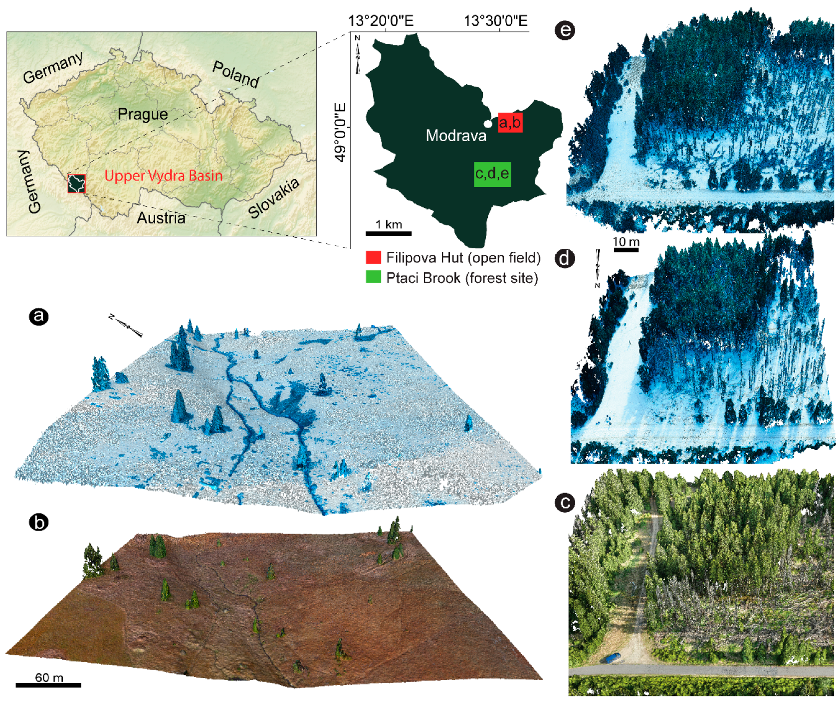
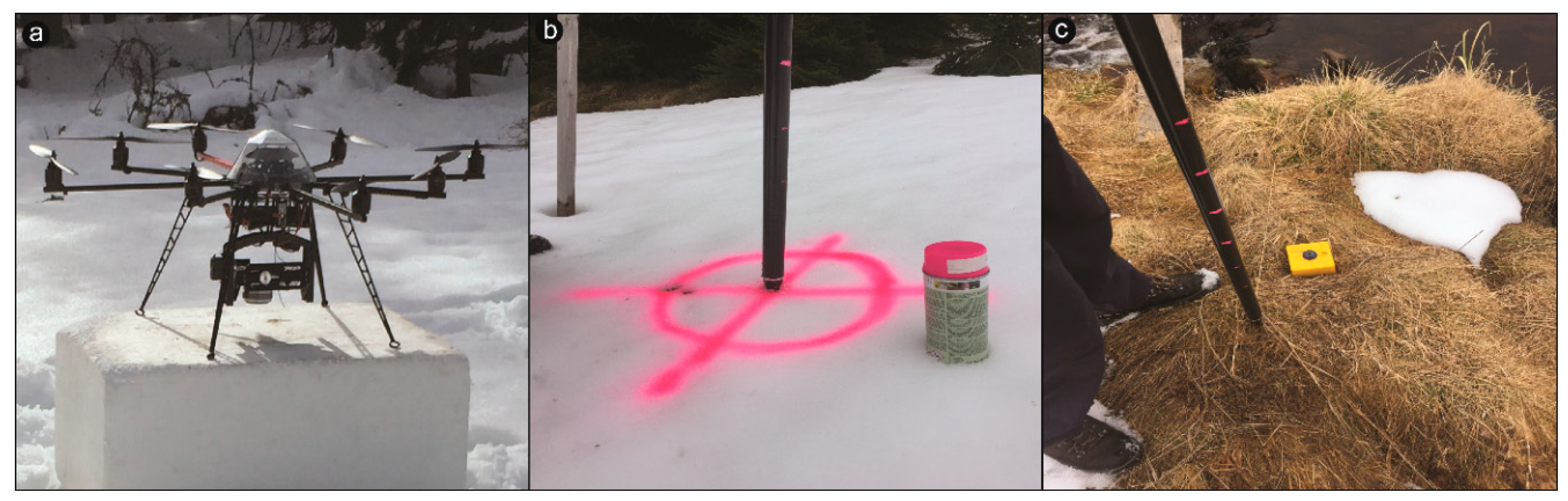
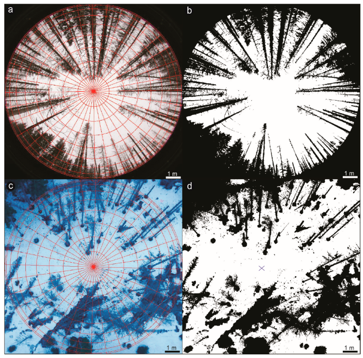
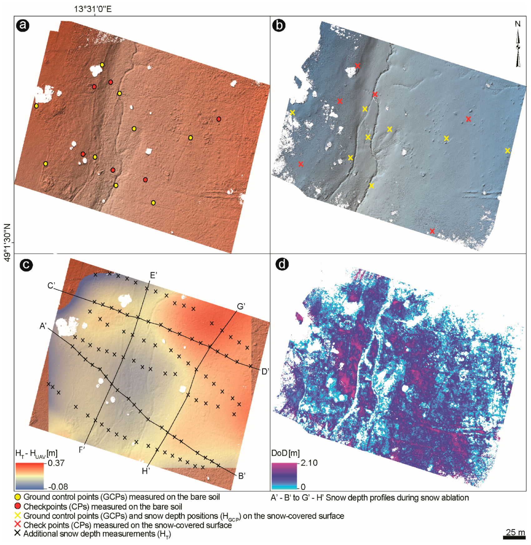
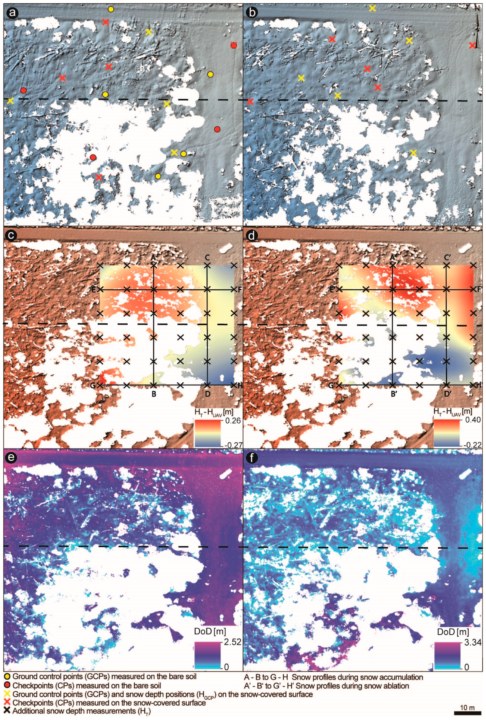
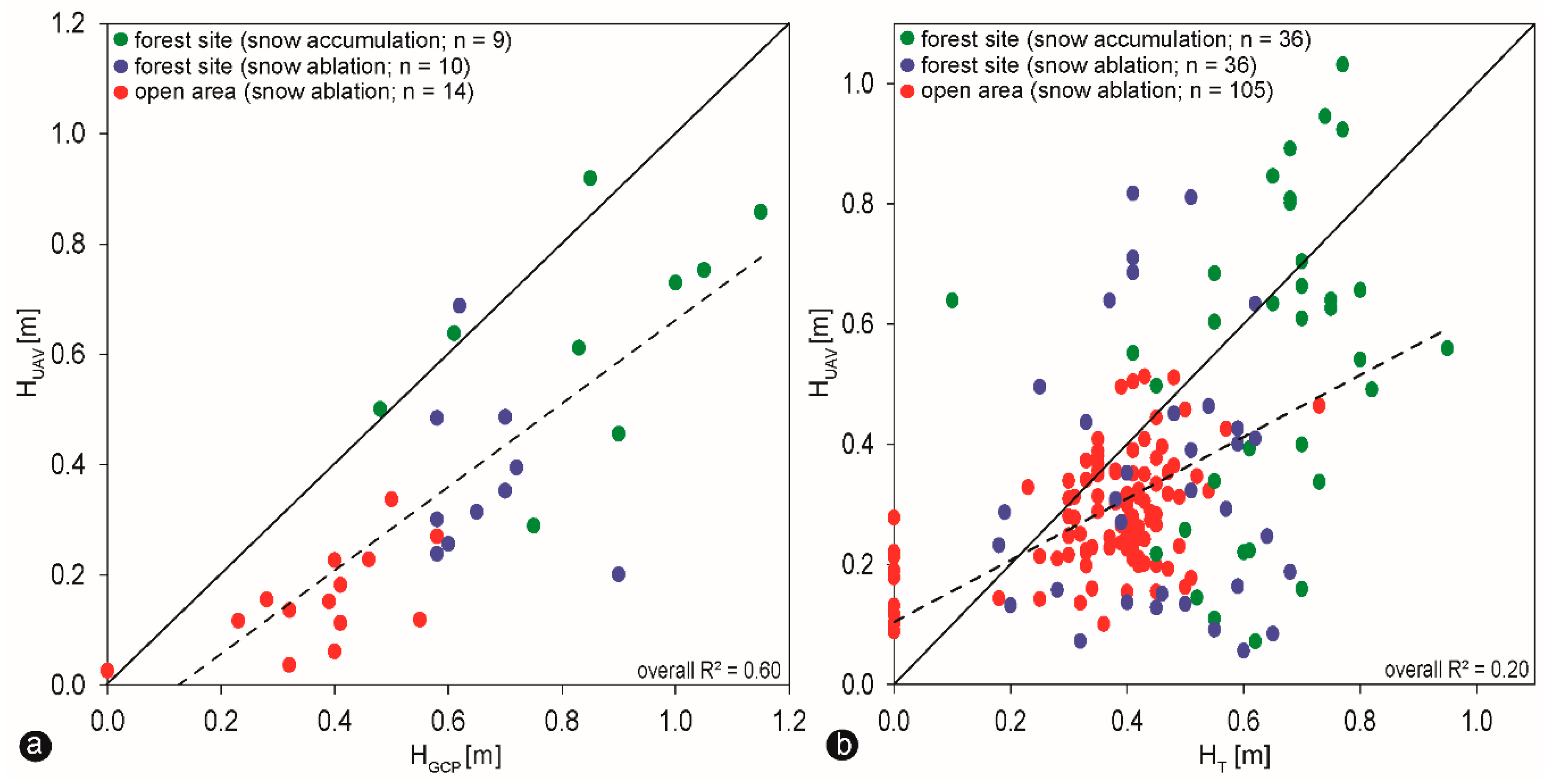
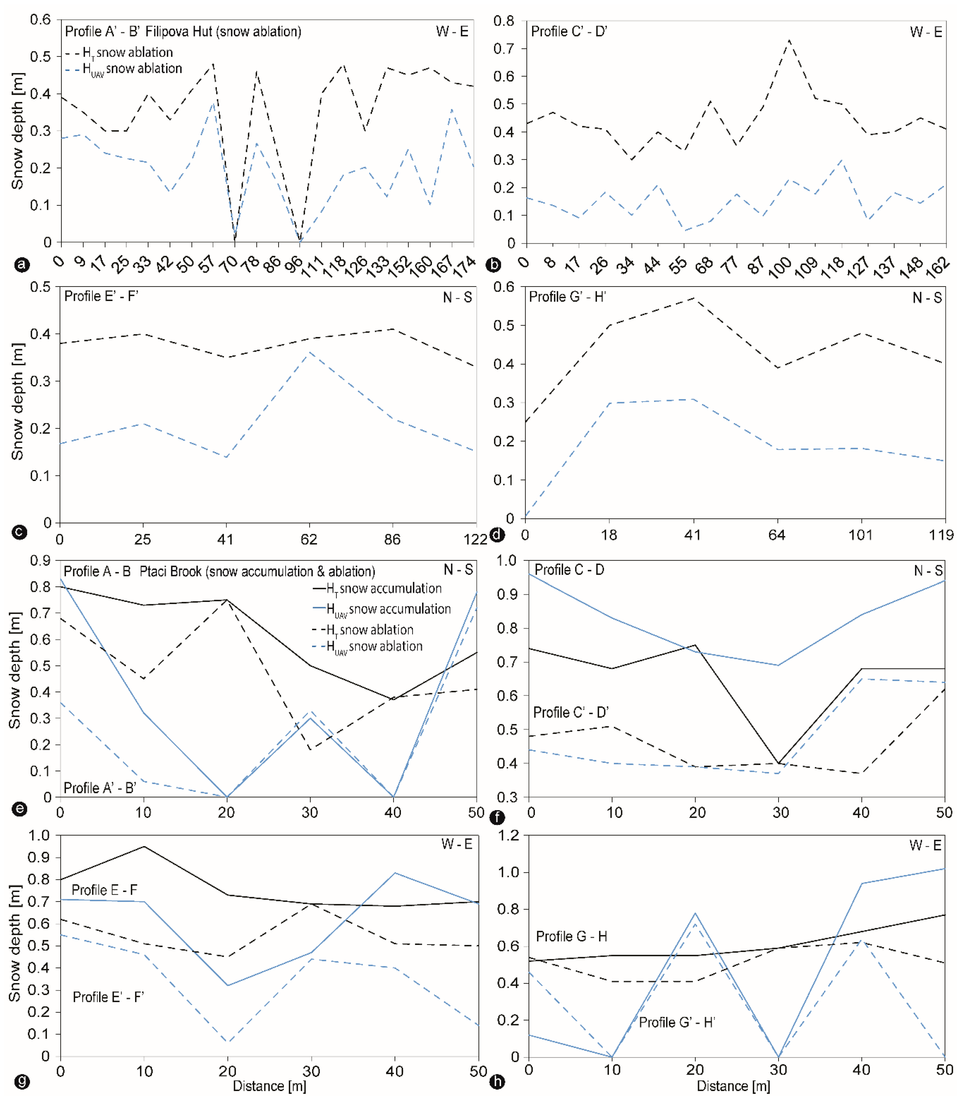
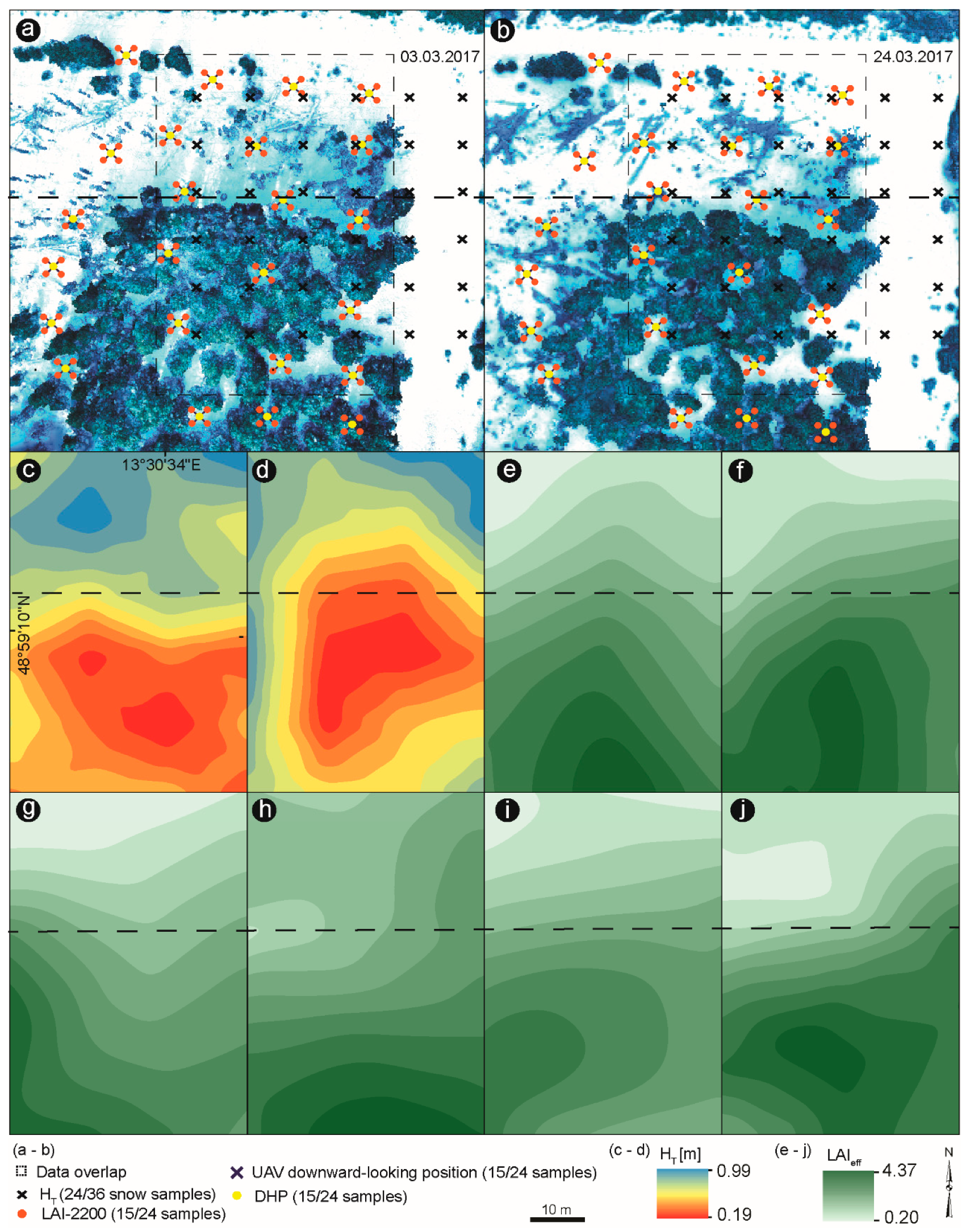
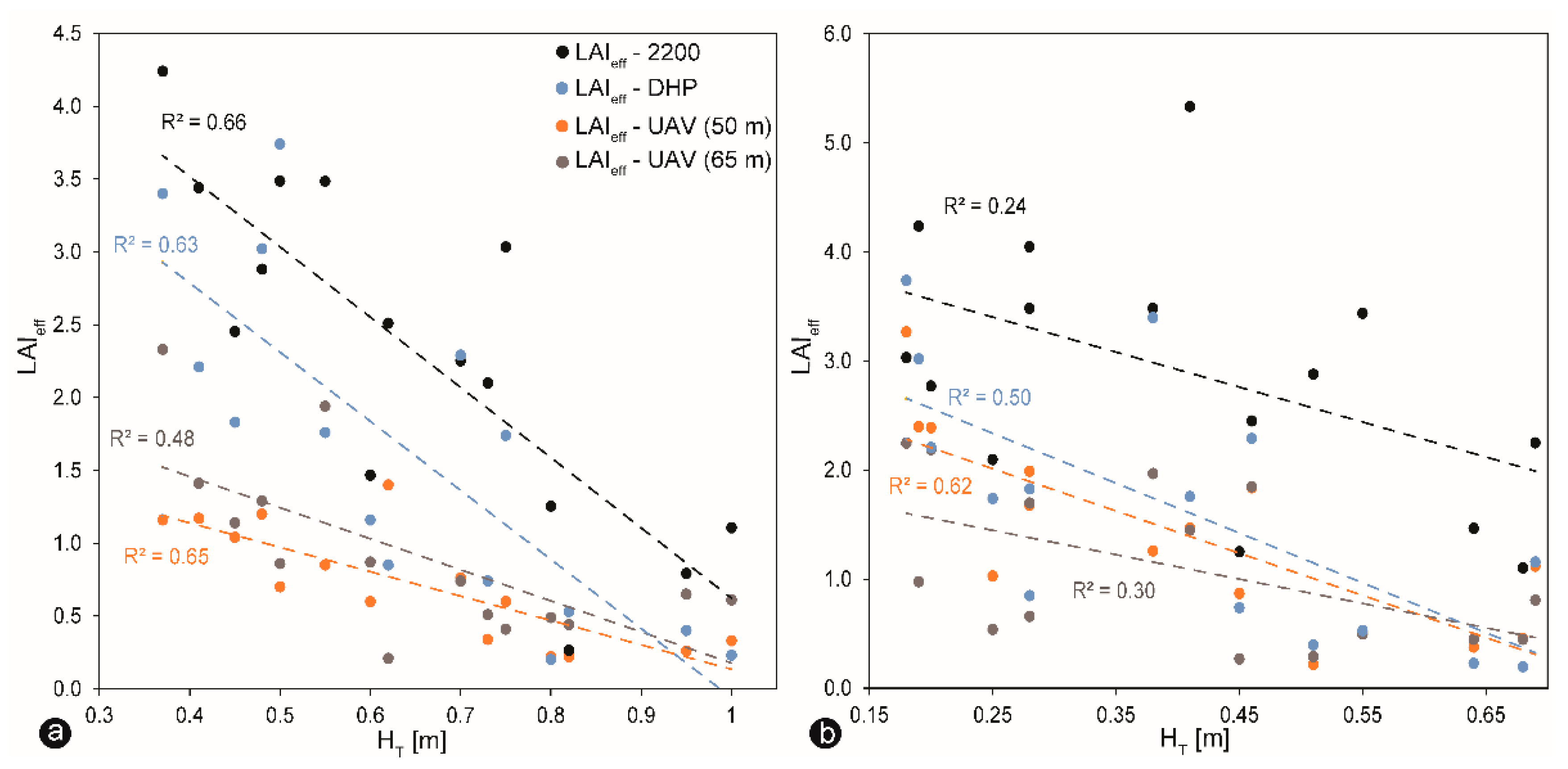
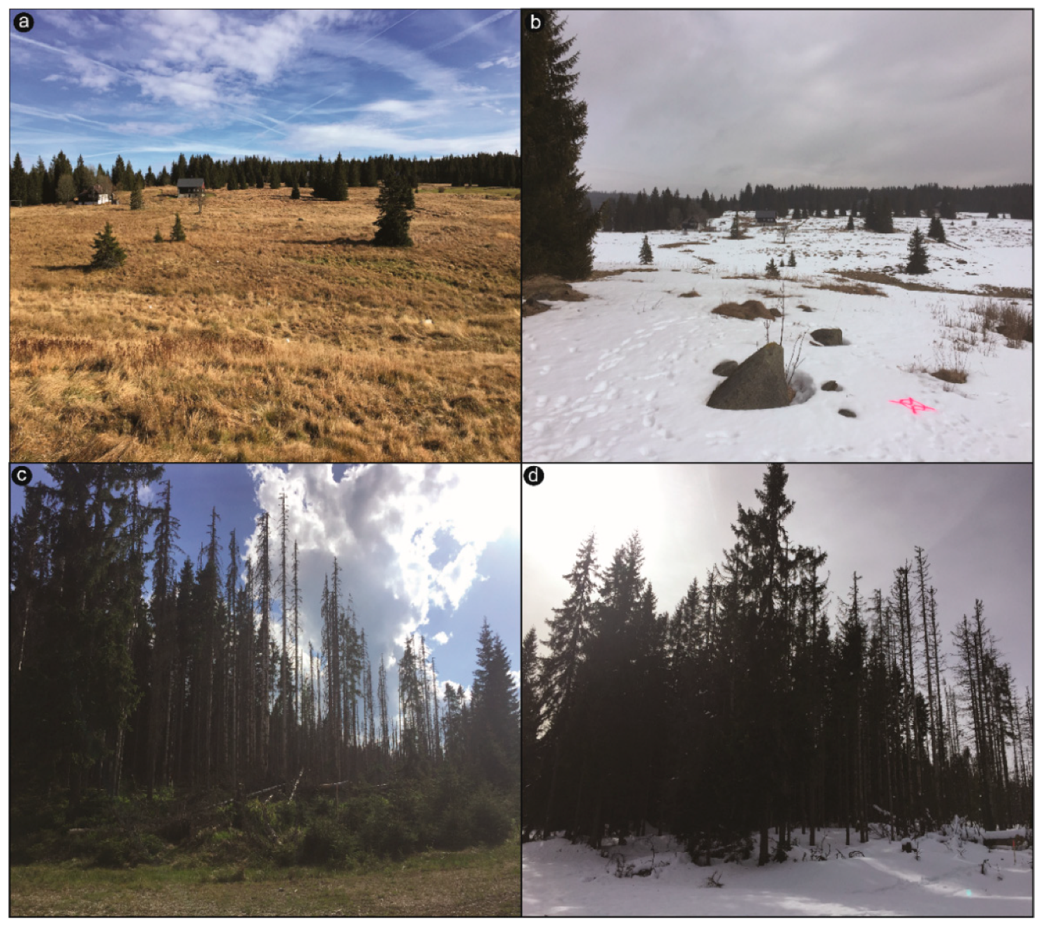
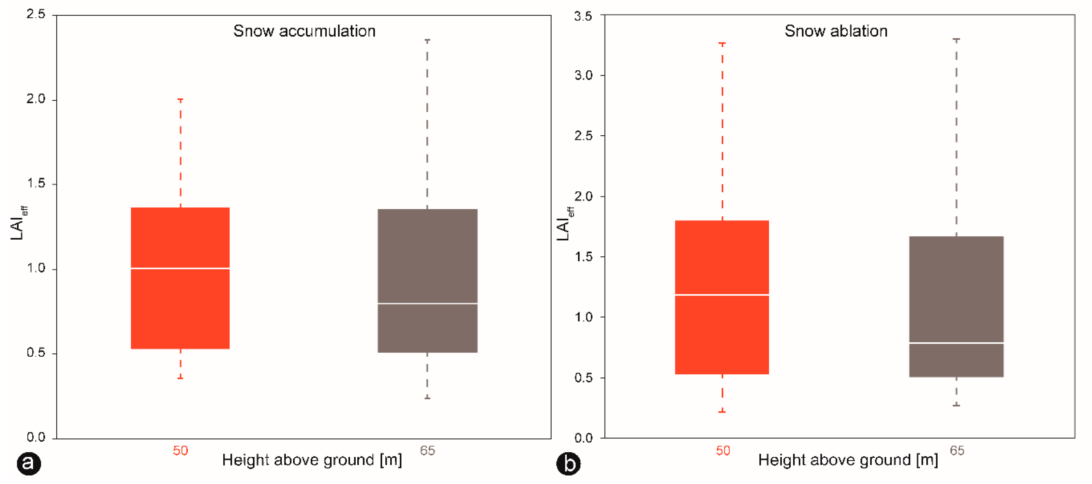
Table 1.
Details about the applied unmanned aerial vehicle (UAV) and camera system.
| UAV Details | |
| UAV type | ARF-OktoXL |
| Dimension | 73 × 73 × 36 |
| Payload | 2500 g |
| Gimbal | MK HiSight SLR2 |
| Max altitude | 100 m |
| Max distance | 100 m |
| Flight time | Max. 45 min |
| Realistic flight time | 15–28 min |
| Navigation | NaviCtrl V2.1 (IMU, barometer, GPS controller), MK-GNSS V4 GPS receiver (American GPS satellites, the European Galileo system, the Russian Glonass satellite or the Chinese BeiDou satellite system) |
| Wireless communication | Graupner MC-32 HoTT remote controller |
| LiPo battery | Vislero 5000, 14.8V 4S1P Flat |
| Camera Details | |
| Camera type | Lumix DMX-GX7 |
| Sensor type | 16MP Live MOS sensor |
| Sensor size (mm) | 17.3 × 13.0 mm (in 4:3 aspect ratio) |
| Focal length | 20 mm |
| Sensor resolution (MP) | 16 |
| ISO range | 125–25,600 |
| Weight (g) | 402 (g) |
Table 2.
Input parameters of GLA. This setting was retained for both fisheye and orthographic image processing.
Table 2.
Input parameters of GLA. This setting was retained for both fisheye and orthographic image processing.
| Input Parameter GLA | Value |
|---|---|
| Cloudiness index | 0.5 |
| Spectral fraction (0.25–25 μm) | 1 |
| Beam fraction | 0.5 |
| Clear-sky transmission coefficient | 0.5 |
| Solar constant (Wm-2) | 1367 |
Table 3.
Summary of the generated point clouds and the digital surface model (DSM) errors compared to the Global Navigation Satellite System (GNSS) elevation at ground control points (GCPs) and picked checkpoint (CP) locations of the open area and forest zone.
Table 3.
Summary of the generated point clouds and the digital surface model (DSM) errors compared to the Global Navigation Satellite System (GNSS) elevation at ground control points (GCPs) and picked checkpoint (CP) locations of the open area and forest zone.
| Flight Campaign | Date | Images | Flight Height [m] | Covered Area [km2] | Mean Ground Resolution [cm/pix] | Number of GCPs | Number of CPs | X Error RMSE [m] | Y Error RMSE [m] | Z Error RMSE [m] | XY Error RMSE [m] | Total RMSE [m] |
|---|---|---|---|---|---|---|---|---|---|---|---|---|
| Filipova Hut (open site; snow ablation) | 24.3. 2017 | 963 | 62.2 | 0.056 | 1.16 | 8 | 6 | 0.041 | 0.039 | 0.055 | 0.056 | 0.079 |
| Filipova Hut (snow-free) | 30.4. 2017 | 1130 | 72.8 | 0.036 | 1.98 | 9 | 6 | 0.066 | 0.035 | 0.036 | 0.075 | 0.084 |
| Ptaci brook (forest site; snow accumulation) | 3.3. 2017 | 906 | 40.3 | 0.012 | 0.73 | 4 | 5 | 0.030 | 0.037 | 0.059 | 0.047 | 0.076 |
| Ptaci brook (snow ablation) | 15.3. 2017 | 1024 | 46 | 0.014 | 0.84 | 5 | 5 | 0.041 | 0.050 | 0.026 | 0.065 | 0.067 |
| Ptaci brook (snow-free) | 30.4. 2017 | 564 | 60.7 | 0.015 | 1.12 | 5 | 4 | 0.046 | 0.030 | 0.056 | 0.055 | 0.078 |
Table 4.
Statistics of the evaluation between estimated (HUAV) snow depths and ground measurements at both study sites. The subtracted HGCP snow depth values from the estimated HUAV measurements are based on one pixel. On the contrary, the subtracted HT samples from the estimated HUAV are based on the mean value within 1 m radius.
| HGCP-HUAV (One Pixel-Base; z values) | Open Area (Snow Ablation) n = 14 | Forest (Snow Accumulation) n = 9 | Forest (Snow Ablation) n = 10 |
| Mean bias [m] | 0.22 | 0.21 | 0.29 |
| SD [m] | 0.11 | 0.19 | 0.19 |
| MAE [m] | 0.09 | 0.16 | 0.13 |
| RMSE [m] | 0.08 | 0.15 | 0.09 |
| HT-HUAV (Mean Value of 1 m Radius; z values) | Open Area (Snow Ablation) n = 105 | Forest (Snow Accumulation) n = 36 | Forest (Snow Ablation) n = 36 |
| Mean bias [m] | 0.08 | 0.14 | 0.14 |
| SD [m] | 0.14 | 0.29 | 0.27 |
| MAE [m] | 0.19 | 0.24 | 0.22 |
| RMSE [m] | 0.16 | 0.32 | 0.31 |
© 2019 by the authors. Licensee MDPI, Basel, Switzerland. This article is an open access article distributed under the terms and conditions of the Creative Commons Attribution (CC BY) license (http://creativecommons.org/licenses/by/4.0/).
Share and Cite
MDPI and ACS Style
Lendzioch, T.; Langhammer, J.; Jenicek, M. Estimating Snow Depth and Leaf Area Index Based on UAV Digital Photogrammetry. Sensors 2019, 19, 1027. https://0-doi-org.brum.beds.ac.uk/10.3390/s19051027
AMA Style
Lendzioch T, Langhammer J, Jenicek M. Estimating Snow Depth and Leaf Area Index Based on UAV Digital Photogrammetry. Sensors. 2019; 19(5):1027. https://0-doi-org.brum.beds.ac.uk/10.3390/s19051027
Chicago/Turabian StyleLendzioch, Theodora, Jakub Langhammer, and Michal Jenicek. 2019. "Estimating Snow Depth and Leaf Area Index Based on UAV Digital Photogrammetry" Sensors 19, no. 5: 1027. https://0-doi-org.brum.beds.ac.uk/10.3390/s19051027
Note that from the first issue of 2016, this journal uses article numbers instead of page numbers. See further details here.