Towards Efficient Electricity Forecasting in Residential and Commercial Buildings: A Novel Hybrid CNN with a LSTM-AE based Framework


Abstract
:1. Introduction

| Category | Paper | Learning Strategy | Dataset | Description |
|---|---|---|---|---|
| Statistical models | [21] | LR | Electricity consumption | Analysis of electricity prediction using LR according to time resolution. |
| [22] | Multiple regression (MR) | Develops two models: ML and genetic algorithm (GA), where GA is used to select critical information from the dataset followed by optimal prediction via the ML model. | ||
| [28] | MR | Uses backward elimination and a multicollinearity process for suitable variable selection and uses a MR model for medium-term electricity prediction. | ||
| Machine learning-based models | [23] | SVR | Electricity load | Adds a temperature variable to improve the performance of SVR for electricity prediction. |
| [24] | Random forest regressor | Electricity consumption | Avoids overfitting by using an ensembled method and transforms the data from time to frequency domain to solve the input data computational complexity. | |
| DL-based models | [25] | Seq2seq | Electricity load | Collects data from real smart meters and develops a sequence-to-sequence-based prediction model for short-term electricity prediction in buildings. |
| [1] | Stacked AE (SAE) | Electricity consumption | Combines SAE with an extreme learning machine (ELM), where SAE is used to extract features and ELM is used as a prediction model. | |
| [29] | DRNN based on pooling | Electricity load | Uses pooling based DRNN, addresses the overfitting problem in a naïve deep learning network and tests the method in a real environment on smart meters in Ireland. | |
| [30] | Seq2seq | Electricity consumption | Uses a sequence-to-sequence model based on modified LSTM. | |
| Hybrid models | [26] | CNN-LSTM | CNNs are used to extract spatial features and LSTM is used for modeling temporal features. | |
| [27] | CNN-bidirectional LSM | CNNs are used to extract spatial features and bidirectional LSTM is used for these features for final prediction. |
- The input dataset is passed through a preprocessing step where redundant, outlier or missing values are removed, and the data are normalized to achieve satisfactory prediction results.
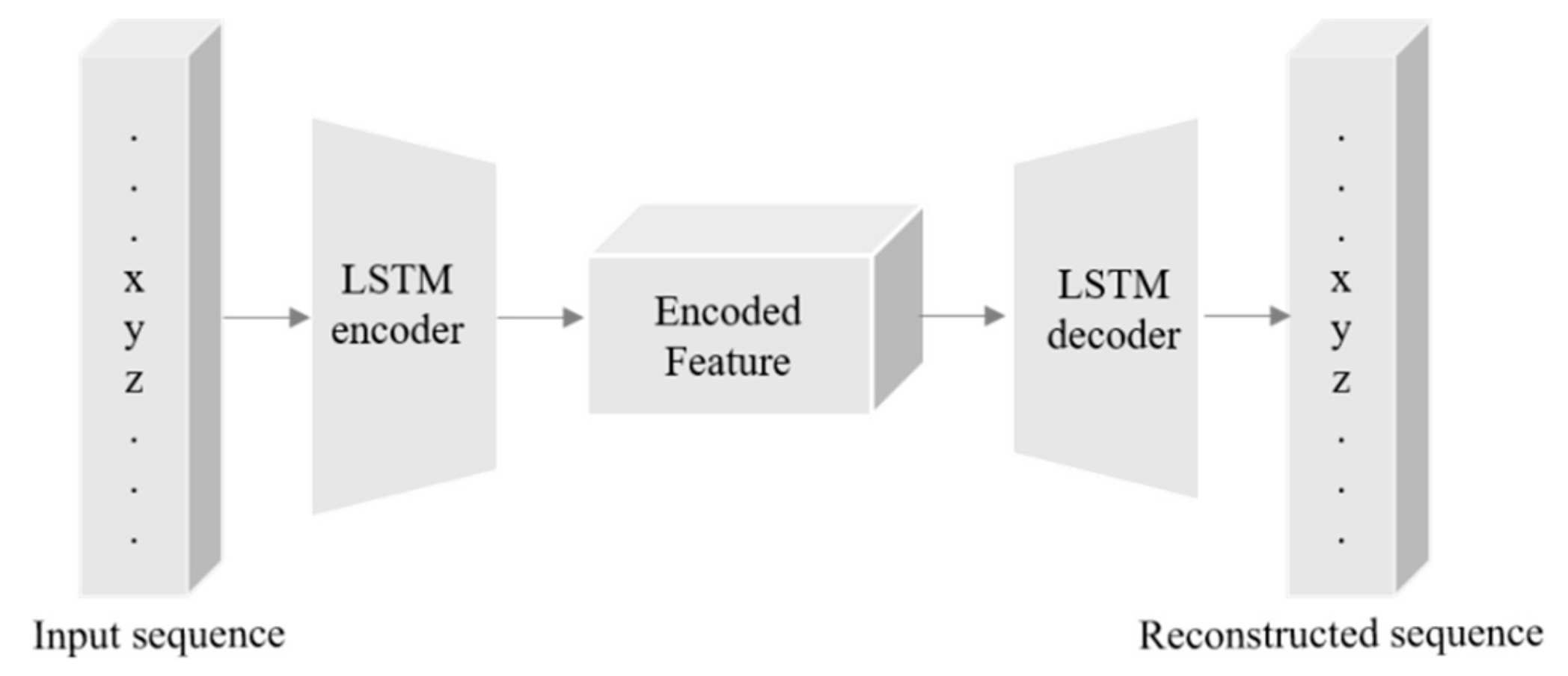
- A novel hybrid model is developed in this work for accurate future energy prediction. The proposed model integrates CNN with LSTM_AE in which the CNN layers are used to extract spatial features from input data and then LSTM-AE are used to model these features.
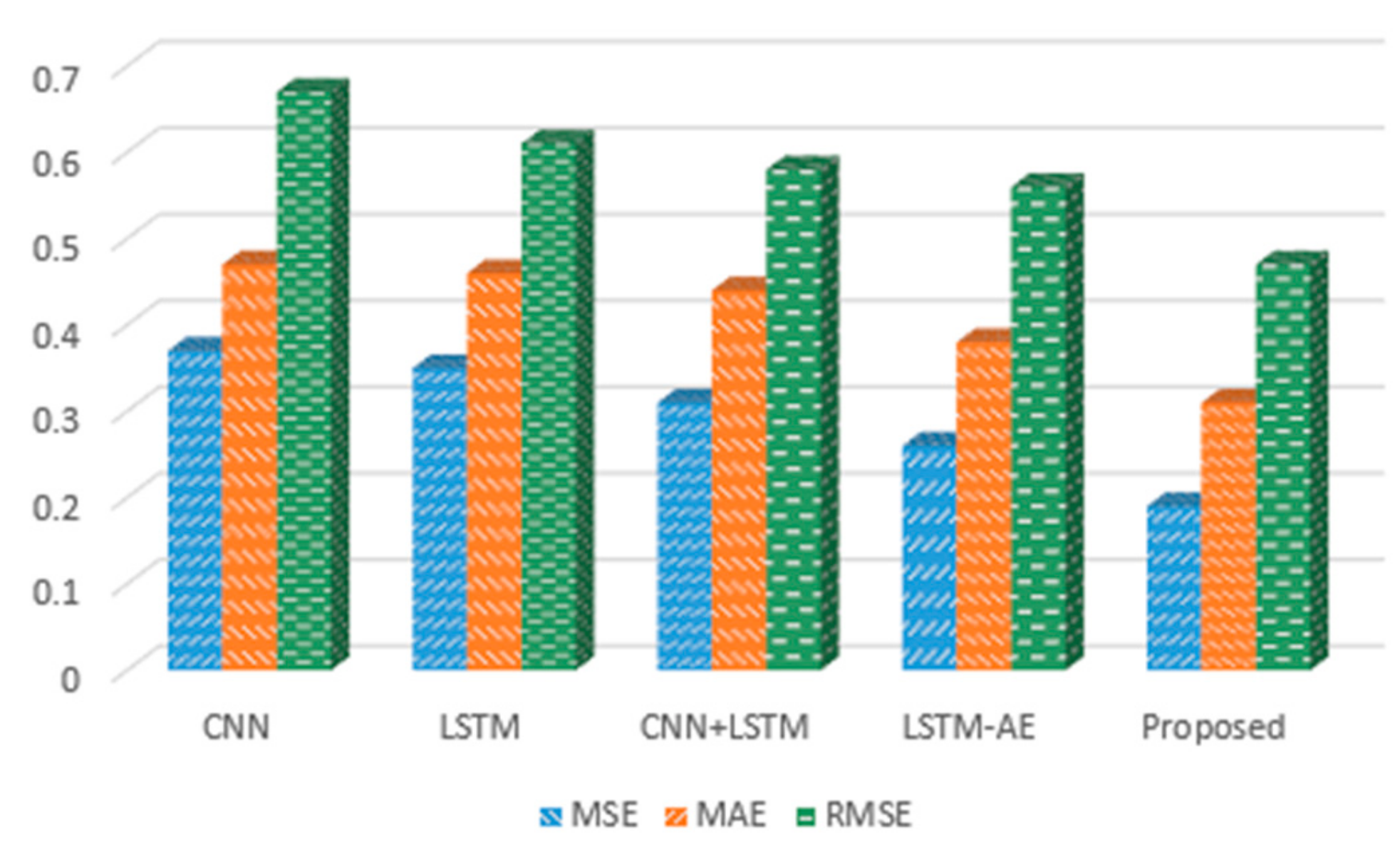
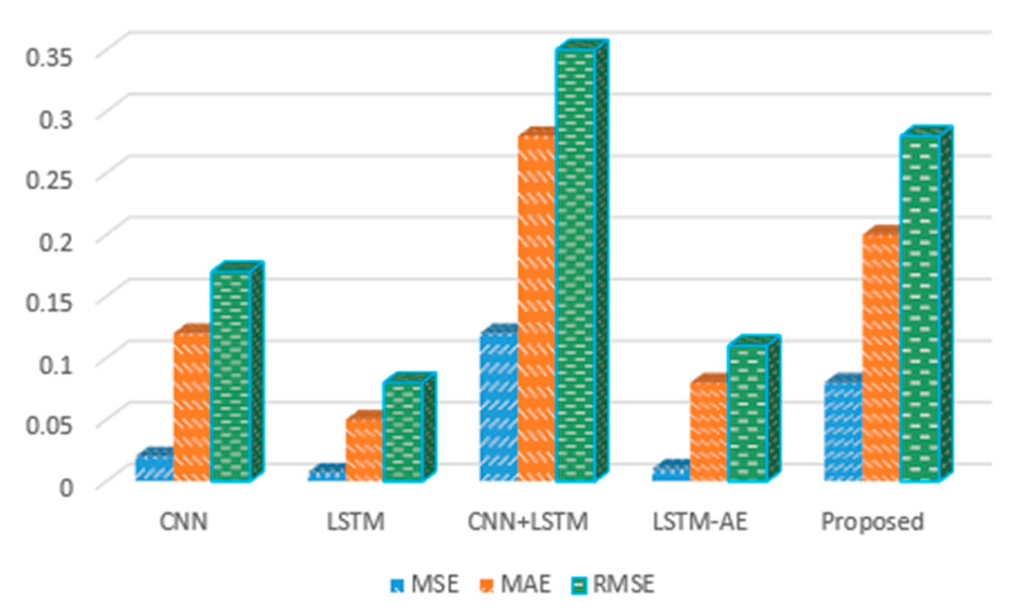
- The experimental results demonstrate that the proposed CNN with LSTM-AE model has the best performance compared to other models. The evaluation metrics record the smallest value for MSE, MAE, RMSE and MAPE for energy consumption prediction.
2. Proposed Framework
2.1. Data Preprocessing
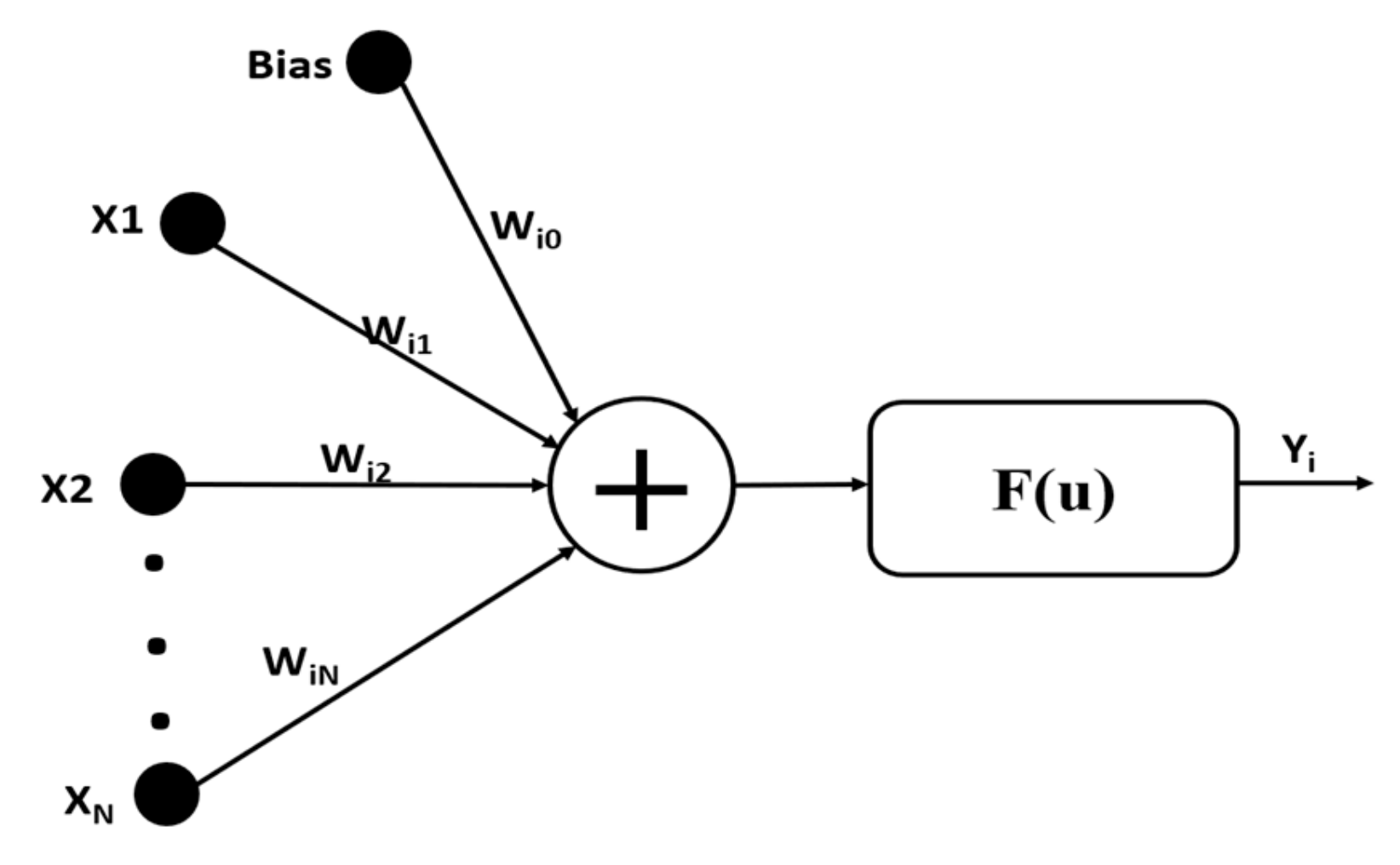
2.2. ANN
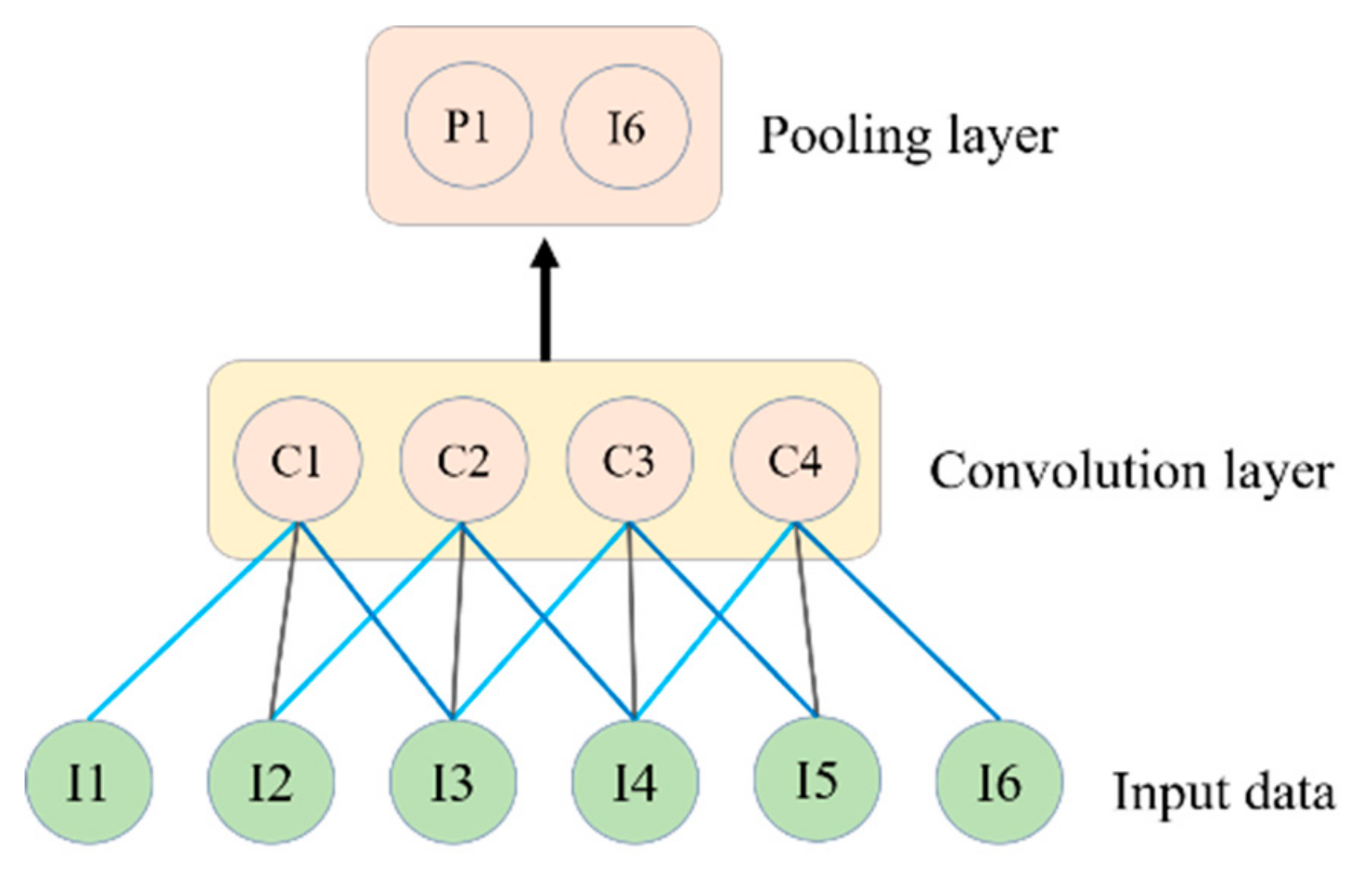
2.3. CNN
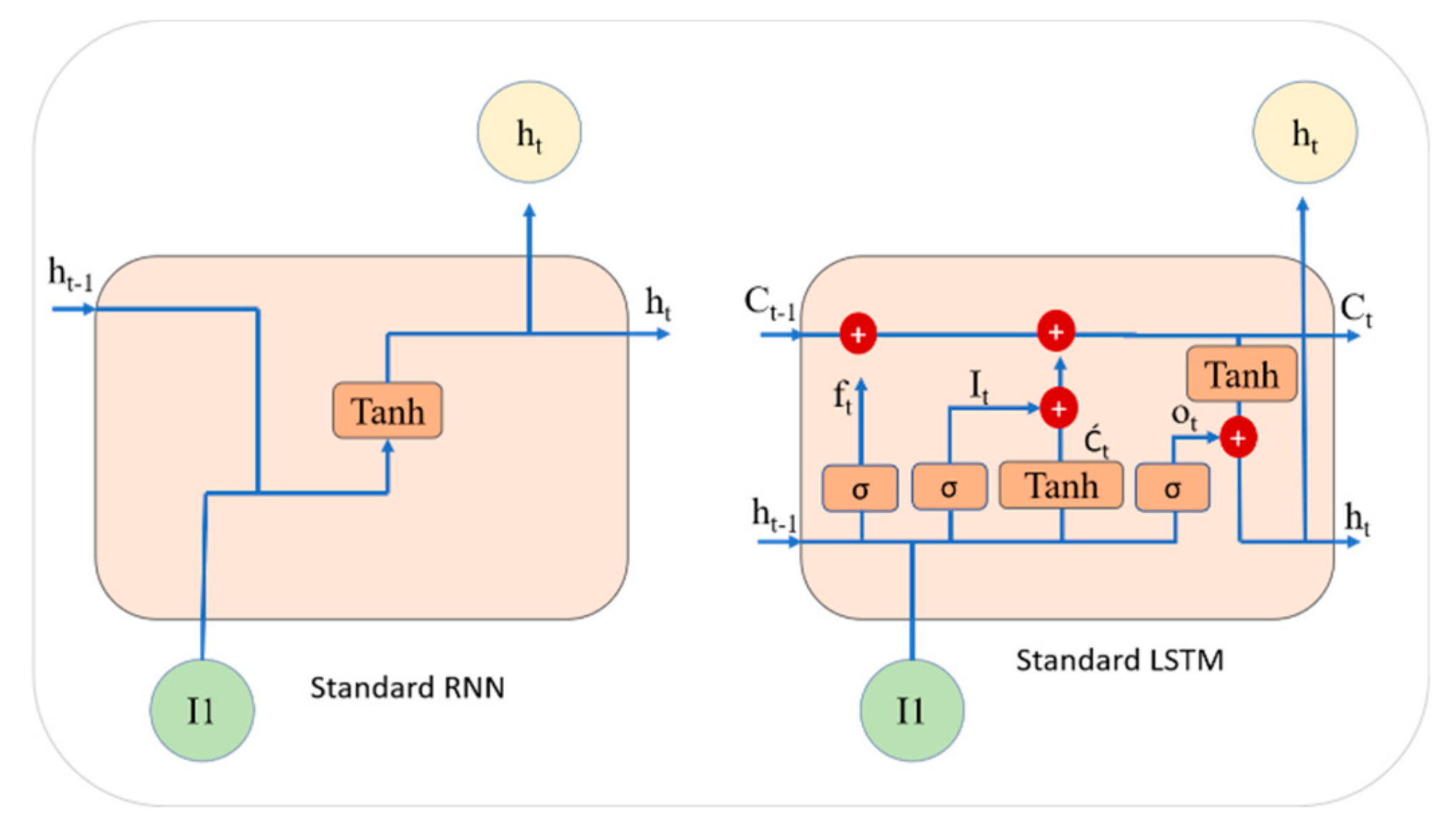
2.4. LSTM
2.5. LSTM-AE
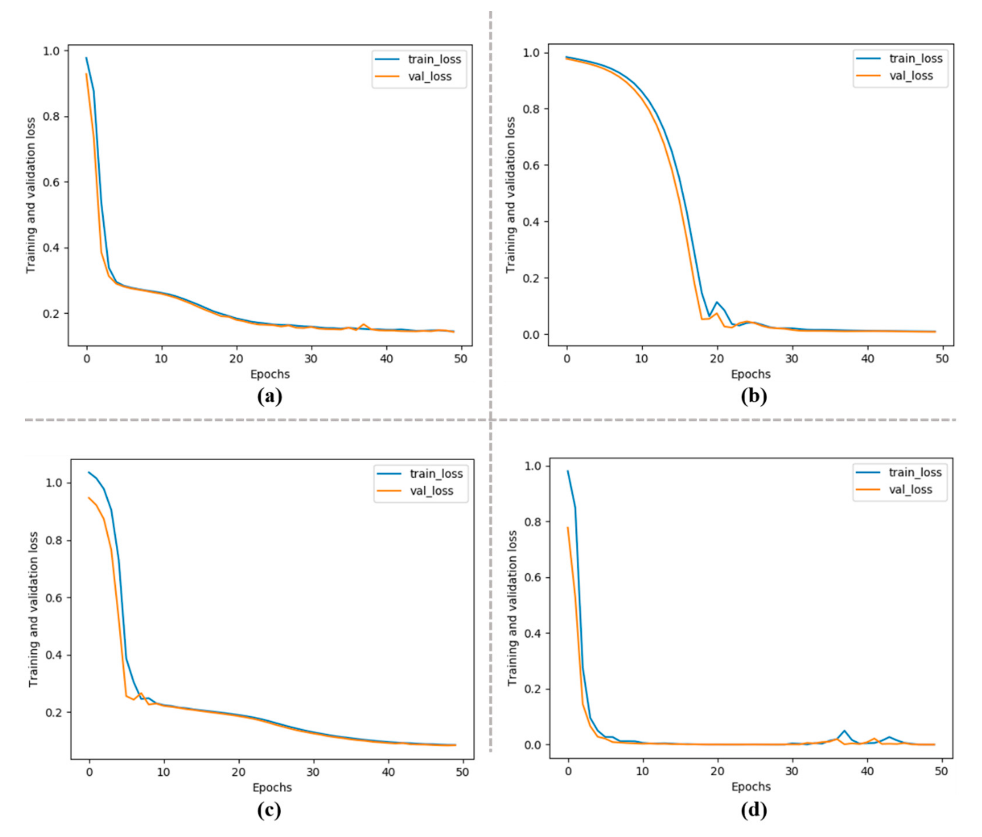
2.6. Training
3. Results
3.1. Experimental Setup
3.2. Datasets
- The UCI dataset was derived from residential buildings while the proposed dataset was generated in commercial buildings.
- The UCI dataset has three consumption sensors: submeters 1, 2 and 3, while our dataset includes only one electricity consumption sensor.
- The UCI dataset includes 1-minute resolution, while the proposed dataset has 15-minute resolution.
3.3. Evaluation Metrics
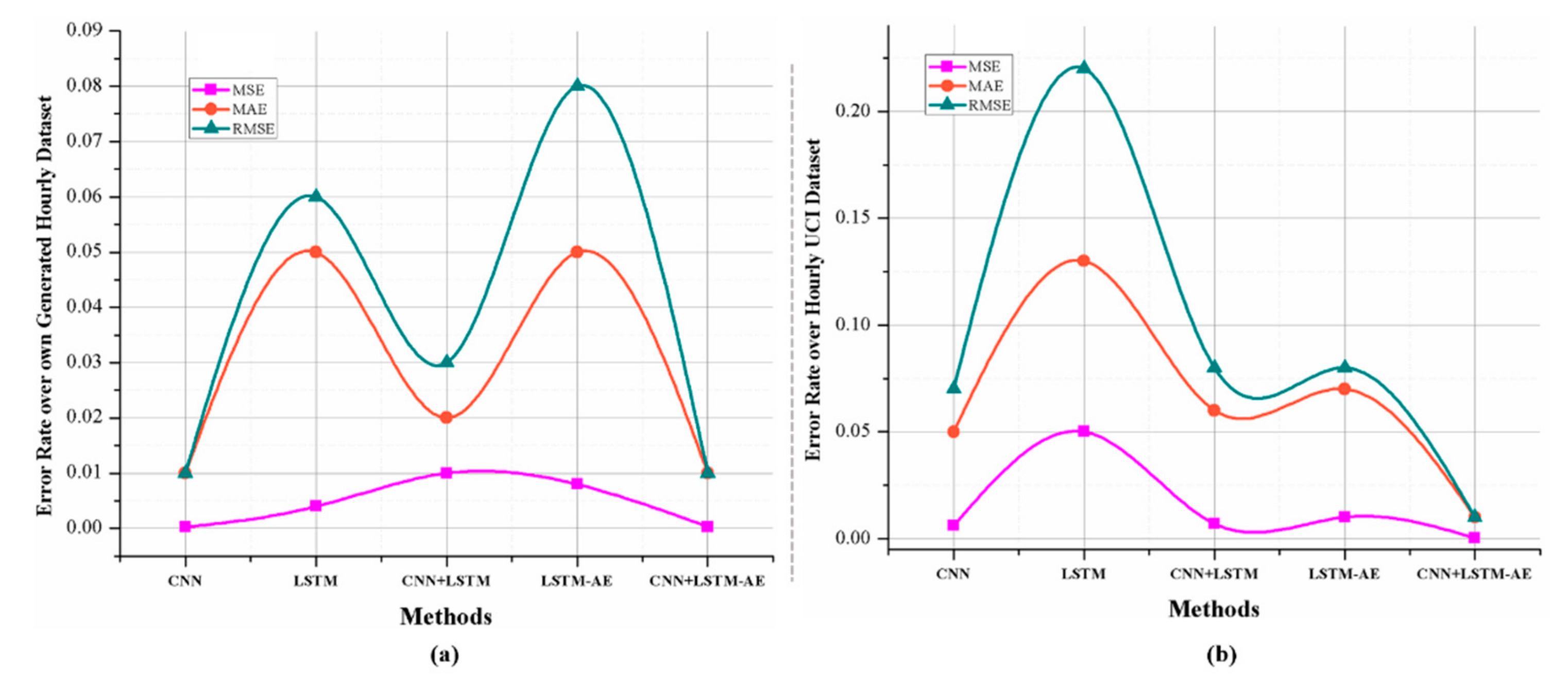
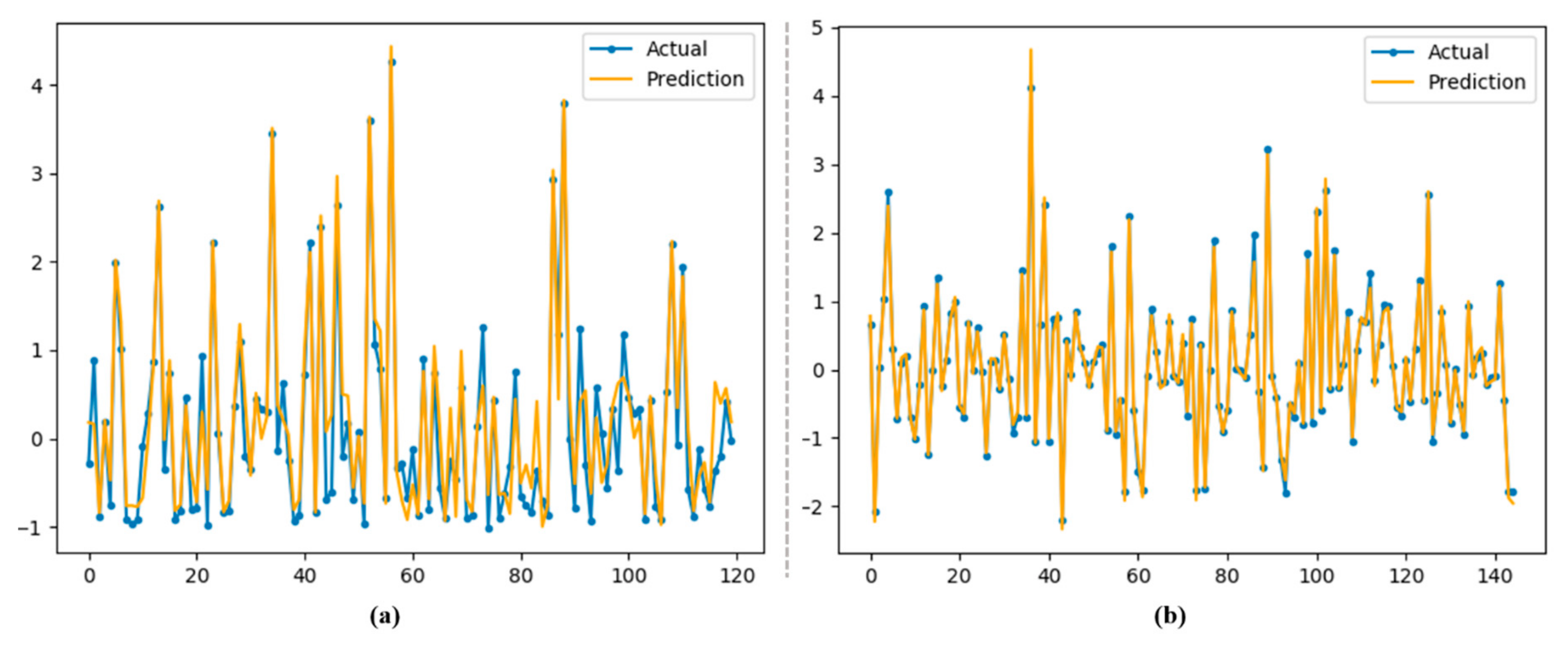
3.4. Performance Evaluation over UCI Dataset
3.5. Performance Evaluation over Newly Generated Dataset
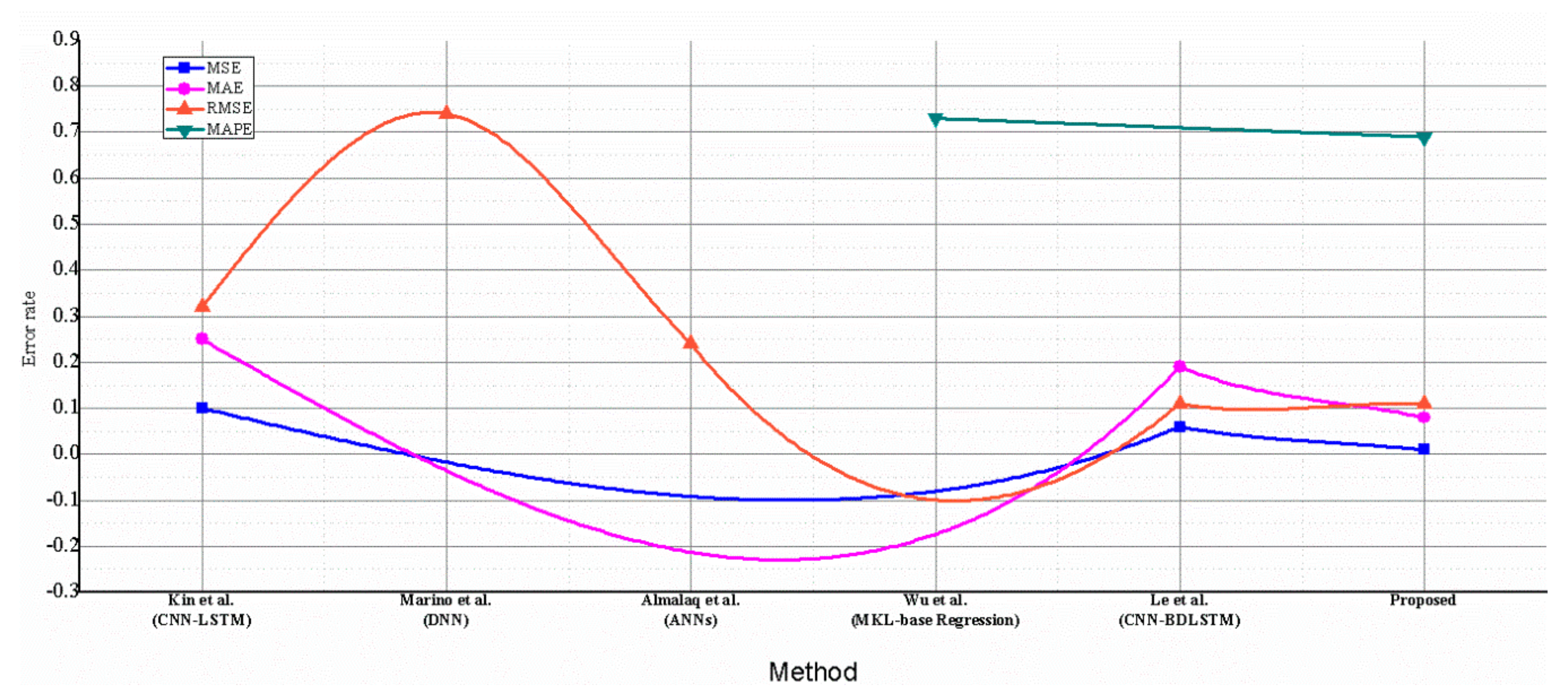
3.6. Comparison with other Baseline Models
4. Conclusions
Author Contributions
Funding
Conflicts of Interest
References
- Li, C.; Ding, Z.; Zhao, D.; Yi, J.; Zhang, G. Building energy consumption prediction: An extreme deep learning approach. Energies 2017, 10, 1525. [Google Scholar] [CrossRef]
- Sieminski, A. International energy outlook. Energy Inf. Adm. (EIA) 2014, 18. [Google Scholar]
- Nejat, P.; Jomehzadeh, F.; Taheri, M.M.; Gohari, M.; Majid, M.Z.A. A global review of energy consumption, CO2 emissions and policy in the residential sector (with an overview of the top ten CO2 emitting countries). Renew. Sustain. Energy Rev. 2015, 43, 843–862. [Google Scholar] [CrossRef]
- Amarasinghe, K.; Wijayasekara, D.; Carey, H.; Manic, M.; He, D.; Chen, W.-P. Artificial neural networks based thermal energy storage control for buildings. In Proceedings of the IECON 2015-41st Annual Conference of the IEEE Industrial Electronics Society, Yokohama, Japan, 9–12 November 2015. [Google Scholar]
- Bunn, D.; Farmer, E.D. Comparative models for electrical load forecasting; Wiley: New York, NY, USA, 1985. [Google Scholar]
- Ullah, A.; Haydarov, K.; Ul Haq, I.; Muhammad, K.; Rho, S.; Lee, M.; Baik, S.W.J.S. Deep Learning Assisted Buildings Energy Consumption Profiling Using Smart Meter Data. Sensors 2020, 20, 873. [Google Scholar] [CrossRef] [PubMed] [Green Version]
- Ullah, F.U.M.; Ullah, A.; Haq, I.U.; Rho, S.; Baik, S.W.J.I.A. Short-Term Prediction of Residential Power Energy Consumption via CNN and Multilayer Bi-directional LSTM Networks; IEEE: Piscataway, NJ, USA, 2019. [Google Scholar]
- Deb, C.; Zhang, F.; Yang, J.; Lee, S.E.; Shah, K.W. A review on time series forecasting techniques for building energy consumption. Renew. Sustain. Energy Rev. 2017, 74, 902–924. [Google Scholar] [CrossRef]
- Kim, K.-H.; Cho, S.-B. Modular Bayesian Networks with Low-Power Wearable Sensors for Recognizing Eating Activities. Sensors 2017, 17, 2877. [Google Scholar]
- Ahmad, M. Seasonal Decomposition of Electricity Consumption Data. Rev. Integr. Bus. Econ. Res. 2017, 6, 271–275. [Google Scholar]
- Hussain, T.; Muhammad, K.; Ullah, A.; Cao, Z.; Baik, S.W.; Albuquerque, V.H.C.d. Cloud-Assisted Multiview Video Summarization Using CNN and Bidirectional LSTM. IEEE Trans. Ind. Inform. 2020, 16, 77–86. [Google Scholar] [CrossRef]
- Kwon, S.J.S. A CNN-Assisted Enhanced Audio Signal Processing for Speech Emotion Recognition. Sensors 2020, 20, 183. [Google Scholar]
- Wang, J.; Yu, L.-C.; Lai, K.R.; Zhang, X. Dimensional sentiment analysis using a regional CNN-LSTM model. In Proceedings of the 54th Annual Meeting of the Association for Computational Linguistics, Berlin, Germany, 7–12 August 2016; Volume 2, Short Papers. pp. 225–230. [Google Scholar]
- Sainath, T.N.; Vinyals, O.; Senior, A.; Sak, H. Convolutional, long short-term memory, fully connected deep neural networks. In Proceedings of the 2015 IEEE International Conference on Acoustics, Speech and Signal Processing (ICASSP), Brisbane, QLD, Australia, 19–24 April 2015; pp. 4580–4584. [Google Scholar]
- Ullah, A.; Ahmad, J.; Muhammad, K.; Sajjad, M.; Baik, S.W. Action recognition in video sequences using deep bi-directional LSTM with CNN features. IEEE Access 2017, 6, 1155–1166. [Google Scholar] [CrossRef]
- Oh, S.L.; Ng, E.Y.; San Tan, R.; Acharya, U.R. Automated diagnosis of arrhythmia using combination of CNN and LSTM techniques with variable length heart beats. Comput. Biol. Med. 2018, 102, 278–287. [Google Scholar] [CrossRef] [PubMed]
- Kaur, H.; Ahuja, S. Time series analysis and prediction of electricity consumption of health care institution using ARIMA model. In Proceedings of the Sixth International Conference on Soft Computing for Problem Solving, Patiala, India, 23–24 December 2016. [Google Scholar]
- Paudel, S.; Elmitri, M.; Couturier, S.; Nguyen, P.H.; Kamphuis, R.; Lacarrière, B.; Le Corre, O. A relevant data selection method for energy consumption prediction of low energy building based on support vector machine. Energy Build. 2017, 138, 240–256. [Google Scholar] [CrossRef]
- Pombeiro, H.; Santos, R.; Carreira, P.; Silva, C.; Sousa, J.M. Comparative assessment of low-complexity models to predict electricity consumption in an institutional building: Linear regression vs. fuzzy modeling vs. neural networks. Energy Build. 2017, 146, 141–151. [Google Scholar] [CrossRef]
- Ascione, F.; Bianco, N.; De Stasio, C.; Mauro, G.M.; Vanoli, G.P. Artificial neural networks to predict energy performance and retrofit scenarios for any member of a building category: A novel approach. Energy 2017, 118, 999–1017. [Google Scholar] [CrossRef]
- Fumo, N.; Biswas, M.R. Regression analysis for prediction of residential energy consumption. Renew. Sustain. Ernergy Rev. 2015, 47, 332–343. [Google Scholar] [CrossRef]
- Amber, K.; Aslam, M.; Hussain, S. Electricity consumption forecasting models for administration buildings of the UK higher education sector. Energy Build. 2015, 90, 127–136. [Google Scholar] [CrossRef]
- Chen, Y.; Xu, P.; Chu, Y.; Li, W.; Wu, Y.; Ni, L.; Bao, Y.; Wang, K. Short-term electrical load forecasting using the Support Vector Regression (SVR) model to calculate the demand response baseline for office buildings. Appl. Energy 2017, 195, 659–670. [Google Scholar] [CrossRef]
- Bogomolov, A.; Lepri, B.; Larcher, R.; Antonelli, F.; Pianesi, F.; Pentland, A. Energy consumption prediction using people dynamics derived from cellular network data. EPJ Data Sci. 2016, 5, 13. [Google Scholar] [CrossRef] [Green Version]
- Kong, W.; Dong, Z.Y.; Jia, Y.; Hill, D.J.; Xu, Y.; Zhang, Y. Short-term residential load forecasting based on LSTM recurrent neural network. IEEE Trans. Smart Grid 2017, 10, 841–851. [Google Scholar] [CrossRef]
- Kim, T.-Y.; Cho, S.-B. Predicting Residential Energy Consumption using CNN-LSTM Neural Networks. Energy 2019. [Google Scholar] [CrossRef]
- Le, T.; Vo, M.T.; Vo, B.; Hwang, E.; Rho, S.; Baik, S.W.J.A.S. Improving electric energy consumption prediction using CNN and Bi-LSTM. Appl. Sci. 2019, 9, 4237. [Google Scholar] [CrossRef] [Green Version]
- Vu, D.H.; Muttaqi, K.M.; Agalgaonkar, A. A variance inflation factor and backward elimination based robust regression model for forecasting monthly electricity demand using climatic variables. Appl. Energy 2015, 140, 385–394. [Google Scholar] [CrossRef] [Green Version]
- Shi, H.; Xu, M.; Li, R. Deep learning for household load forecasting—A novel pooling deep RNN. IEEE Transact. Smart Grid 2017, 9, 5271–5280. [Google Scholar] [CrossRef]
- Marino, D.L.; Amarasinghe, K.; Manic, M. Building energy load forecasting using deep neural networks. In Proceedings of the IECON 2016-42nd Annual Conference of the IEEE Industrial Electronics Society, Florence, Italy, 23–26 October 2016; pp. 7046–7051. [Google Scholar]
- Orbach, J. Principles of Neurodynamics. Perceptrons and the Theory of Brain Mechanisms. Arch. Gen. Psychiatry 1962, 7, 218–219. [Google Scholar] [CrossRef]
- LeCun, Y.; Bengio, Y. Convolutional networks for images, speech, and time series. The handbook of brain theory and neural networks; MIT Press: Cambridge, MA, USA, 1995. [Google Scholar]
- Qiu, Z.; Chen, J.; Zhao, Y.; Zhu, S.; He, Y.; Zhang, C. Variety identification of single rice seed using hyperspectral imaging combined with convolutional neural network. Appl. Sci. 2018, 8, 212. [Google Scholar] [CrossRef] [Green Version]
- Li, C.; Zhou, H. Enhancing the efficiency of massive online learning by integrating intelligent analysis into MOOCs with an application to education of sustainability. Sustainability 2018, 10, 468. [Google Scholar] [CrossRef] [Green Version]
- An, Q.; Pan, Z.; You, H. Ship detection in Gaofen-3 SAR images based on sea clutter distribution analysis and deep convolutional neural network. Sensors 2018, 18, 334. [Google Scholar] [CrossRef] [Green Version]
- Hochreiter, S.; Schmidhuber, J. Long short-term memory. Neural Comput. 1997, 9, 1735–1780. [Google Scholar] [CrossRef]
- Sutskever, I.; Vinyals, O.; Le, Q.V. Sequence to sequence learning with neural networks. In Proceedings of the Advances in neural information processing systems; NIPS: San Diego, CA, USA; pp. 3104–3112.
- UCI. Individual household electric power consumption Data Set. Available online: https://archive.ics.uci.edu/ml/datasets/individual+household+electric+power+consumption (accessed on 4 March 2020).
- Kim, J.-Y.; Cho, S.-B. Electric energy consumption prediction by deep learning with state explainable autoencoder. Energies 2019, 12, 739. [Google Scholar] [CrossRef] [Green Version]
- Almalaq, A.; Edwards, G. Comparison of Recursive and Non-Recursive ANNs in Energy Consumption Forecasting in Buildings. In Proceedings of the 2019 IEEE Green Technologies Conference (GreenTech), Lafayette, LA, USA, 3–6 April 2019; pp. 1–5. [Google Scholar]
- Wu, D.; Wang, B.; Precup, D.; Boulet, B.J.I.T.o.S.G. Multiple Kernel Learning based Transfer Regression for Electric Load Forecasting; IEEE: Piscataway, NJ, USA, 2019. [Google Scholar]
- Chujai, P.; Kerdprasop, N.; Kerdprasop, K. Time series analysis of household electric consumption with ARIMA and ARMA models. In Proceedings of the International MultiConference of Engineers and Computer Scientist, Hong Kong, China, 13–15 March 2013; pp. 295–300. [Google Scholar]
- Rajabi, R.; Estebsari, A. Deep Learning Based Forecasting of Individual Residential Loads Using Recurrence Plots. In Proceedings of the 2019 IEEE Milan PowerTech, Milan, Italy, 23–27 June 2019; pp. 1–5. [Google Scholar]


| Variable | Description |
|---|---|
| Date | Presented in dd/mm/yyyy format. |
| Time | Time variable given in hours, minutes and seconds (hh:mm:ss) |
| Global active power | Minutely given average active and reactive power for individual house. |
| Global active power | |
| Voltage | One-minute average voltage |
| Intensity | Current intensity for every minute. |
| Submetering (1, 2, 3) | Active electricity related to kitchen, laundry room and living room of residential home, while only one submetering_1 sensor in commercial dataset is related to office electricity. |
| Methods | MSE | MAE | RMSE | MAPE | |
|---|---|---|---|---|---|
| Deep Learning Methods | Kim, T.-Y et al. [26] | 0.35 | 0.33 | 0.59 | - |
| Kim, J, -Y et al. [39] | 0.38 | 0.39 | - | - | |
| Marino et al. [30] | - | - | 0.74 | - | |
| Le et al. [27] | 0.29 | 0.39 | 0.54 | - | |
| Traditional Machine Learning models | ARMA [42] | - | - | 0.30 | - |
| SVM [43] | - | 1.12 | 1.25 | - | |
| Linear Regression [41] | - | - | - | 1.03 | |
| SVR [41] | - | - | - | 1.29 | |
| Gaussian Process [41] | - | - | - | 0.82 | |
| Proposed | 0.19 | 0.31 | 0.47 | 0.76 |
© 2020 by the authors. Licensee MDPI, Basel, Switzerland. This article is an open access article distributed under the terms and conditions of the Creative Commons Attribution (CC BY) license (http://creativecommons.org/licenses/by/4.0/).
Share and Cite
Khan, Z.A.; Hussain, T.; Ullah, A.; Rho, S.; Lee, M.; Baik, S.W. Towards Efficient Electricity Forecasting in Residential and Commercial Buildings: A Novel Hybrid CNN with a LSTM-AE based Framework. Sensors 2020, 20, 1399. https://0-doi-org.brum.beds.ac.uk/10.3390/s20051399
Khan ZA, Hussain T, Ullah A, Rho S, Lee M, Baik SW. Towards Efficient Electricity Forecasting in Residential and Commercial Buildings: A Novel Hybrid CNN with a LSTM-AE based Framework. Sensors. 2020; 20(5):1399. https://0-doi-org.brum.beds.ac.uk/10.3390/s20051399
Chicago/Turabian StyleKhan, Zulfiqar Ahmad, Tanveer Hussain, Amin Ullah, Seungmin Rho, Miyoung Lee, and Sung Wook Baik. 2020. "Towards Efficient Electricity Forecasting in Residential and Commercial Buildings: A Novel Hybrid CNN with a LSTM-AE based Framework" Sensors 20, no. 5: 1399. https://0-doi-org.brum.beds.ac.uk/10.3390/s20051399