Effects on Public Health of Heat Waves to Improve the Urban Quality of Life

Abstract

Life satisfaction has been widely used in recent studies to evaluate the effect of environmental factors on individuals’ well-being. In the last few years, many studies have shown that the potential impact of climate change on cities depends on a variety of social, economic, and environmental determinants. In particular, extreme events, such as flood and heat waves, may cause more severe impacts and induce a relatively higher level of vulnerability in populations that live in urban areas. Therefore, the impact of climate change and related extreme events certainly influences the economy and quality of life in affected cities. Heat wave frequency, intensity, and duration are increasing in global and local climate change scenarios. The association between high temperatures and morbidity is well-documented, but few studies have examined the role of meteo-climatic variables on hospital admissions. This study investigates the effects of temperature, relative humidity, and barometric pressure on health by linking daily access to a Matera (Italy) hospital with meteorological conditions in summer 2012. Extreme heat wave episodes that affected most of the city from 1 June to 31 August 2012 (among the selected years 2003, 2012, and 2017) were analyzed. Results were compared with heat waves from other years included in the base period (1971–2000) and the number of emergency hospital admissions on each day was considered. The meteorological data used in this study were collected from two weather stations in Matera. In order to detect correlations between the daily emergency admissions and the extreme health events, a combined methodology based on a heat wave identification technique, multivariate analysis (PCA), and regression analysis was applied. The results highlight that the role of relative humidity decreases as the severity level of heat waves increases. Moreover, the combination of temperatures and daily barometric pressure range (DPR) has been identified as a precursor for a surveillance system of risk factors in hospital admissions.

1. Introduction

Climate change is a major public health threat due to the effects of extreme weather events on human health and on quality of life in general [1,2,3,4]. In the last three decades, many studies have addressed the issue of climate evolution under anthropic pressure and the relative increase of its effects observed in the last century [5,6,7]. Recently, several studies have suggested that heat exposure reduces emotional wellbeing, increases interpersonal aggression, and diminishes life satisfaction [8,9,10]. In fact, heat exposure is associated with increased suicide rates [11,12,13]. Together, these findings indicate that heat exposure may adversely impact mental health and that global climate change, by increasing exposure to extreme heat, could similarly have negative consequences for physical and mental health [2]. A critical literature review on the definition of heat waves, on the impacts of heat waves on health, ecosystems, and the built environment, and on the current mechanisms to deal with impacts of heat waves was reported by Zou et al. [14].

Climate warming, as noted over the past several decades, is consistently associated with changes in a number of components of the hydrological cycle and hydrological systems, such as: changing precipitation patterns, intensity, and extremes; causing a widespread melting of snow and ice; increasing atmospheric water vapor; increasing evaporation; and causing changes in soil moisture and runoff [15].

In this context, mean temperatures are increasing, in particular extreme temperatures, with heat waves (HWs) becoming more frequent, more intense, and longer lasting. In many cities, extreme HWs have drastically increased [16,17]. In an urban area, this effect, called the urban heat island (UHI) phenomenon, may raise the temperature by as much as 10 °C due to different local environments and atmospheric conditions [18].

Several studies carried out in the United States assert that HWs led to the highest 10-year estimates of fatalities and the second-greatest estimated economic damage (after hurricanes) among the main weather and climate disaster events in the USA from 2004 to 2013 [19,20]. In general, HW phenomena are one of the natural hazards with the greatest impact worldwide in terms of mortality and economic losses. [21,22]. In the last 15 years, Europe has suffered a high number of severe summer HWs with devastating health and economic effects. Out of the last 15 years, 2003, 2006, 2007, 2013, 2014, and 2015 should be mentioned due to the major HW events that occurred in Europe for their great magnitude, spatial area, and temporal persistence measured in consecutive days [23,24,25,26,27]. Most of these HWs were included in the top ten HWs that have occurred in Europe since 1950 [20].

In Italy, the summer of 2012 was characterized by high average temperatures (+2.3 °C compared to the period 1970–1999), enough to be considered one of the hottest summers since 1800; since 2000, it was the hottest after the summer of 2003 (with +3.7 °C) [28].

The intensity, duration, and timing of HWs can influence the risk of heat-related mortality. In the EuroHEAT study of the health effects of HWs in a number of European cities, it was found that in prolonged HW events, mortality was 1.5–5 times higher than for HWs of short duration, with the highest increases for prolonged heat events found in several cities (Athens, Budapest, London, Rome, and Valencia) in the 75+ age group [29,30,31]. There are various approaches to detecting climate variations on a local scale. Common methods include the use of climate data and their analysis with satellite imagery or mathematical modeling that compares a climate variable or an indicator between different locations at different local scales [32,33,34,35]. Recent studies report on the use of satellite monitoring of extreme heat events in urban areas and estimations of associated public health impact. Satellite thermal data can depict the spatial gradient of radiometric surface (and not ambient) temperature [36].

Detailed observations and monitoring, as well as real-time dissemination of meteo-climatic information, quantification by remote sensing (radar and satellites), and derived indices and operational services are important for decision development plans in different contexts (public health, agricultural, water resources, energy), for example in terms of managing and optimizing data monitoring networks [37,38].

The present study examines the interactions between heat waves and daily-diagnosis-related emergency admission to the hospital in Matera in the period June 2012 to August 2012. In particular, the focus was on temperatures, relative humidity, and variations of barometric pressure through the combination of multivariate statistical techniques and linear multiple regression analysis.

In this study, identification of a heat wave day was based on the suggestion made by the Intergovernmental Panel on Climate Change (IPCC) to define an extreme weather event. The World Meteorological Organization (WMO) defines HWs as periods of at least six days with a maximum temperature exceeding the 90th percentile of daily maximum temperature calculated on each calendar day in the base period CLINOs (Climatological Normals), the average values of meteorological elements for a 30-year period (1961–1990 or 1971–2000) [39,40].

Multivariate statistical analysis allows rapid definition of descriptor profiles and their interpretation in terms of the measured variables. In particular, Principal Component Analysis (PCA) is a dimension-reduction tool that can be used to reduce a large set of variables by transforming the dataset into a smaller number of artificial variables (called principal components) that will account for most of the variance of the observed variables.

In order to reduce the number of weather variables collected at the meteo-climatic stations and to define their correlation structure with the number of emergency hospital admissions on each day, PCA was applied in the present investigation [37,41,42,43].

2. Data Source

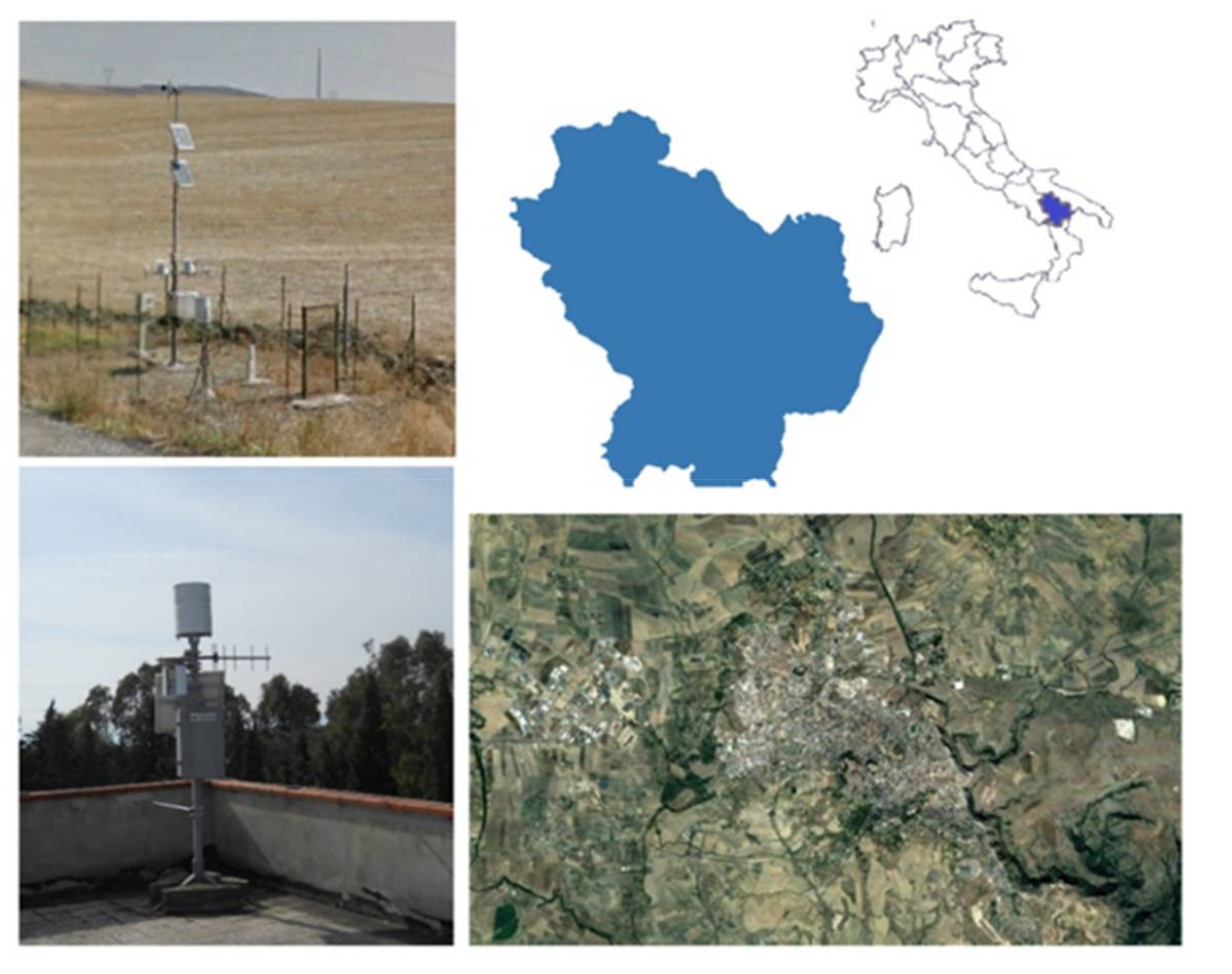
The study was conducted in Matera, located in southern Italy. In 2015, Matera was home to approximately 60,500 citizens in an area of about 390 km². The city attracts many visitors, causing an increase in population fluctuation, especially in summer, of approximately 300% from 2000 to 2015. Matera presents a typical Mediterranean climate with mild winters and hot humid summers, with an annual average temperature of 14 °C and average humidity of 65%.

Data were collected from two representative meteorological stations (see Figure 1). They were chosen according to type and significant duration of variables of interest in the study area:

MTA (MaTera Alsia): A historical monitoring station managed by the regional Agency for Development and Innovation in Agriculture (Italian acronym, ALSIA); hourly air temperatures (maximum and minimum) and precipitation, from 1918 to present;

MTCP (MaTera Civil Protection): an urban station managed by the National Civil Protection Department; sub-hourly summer data of maximum and minimum temperatures (°C), maximum and minimum relative humidity (%), and maximum and minimum barometric pressure (hPa), from 2000 to present.

Daily admissions data were made available by the emergency department of the Matera hospital “Madonna delle Grazie” from 1 June 2012 to 31 August 2012.

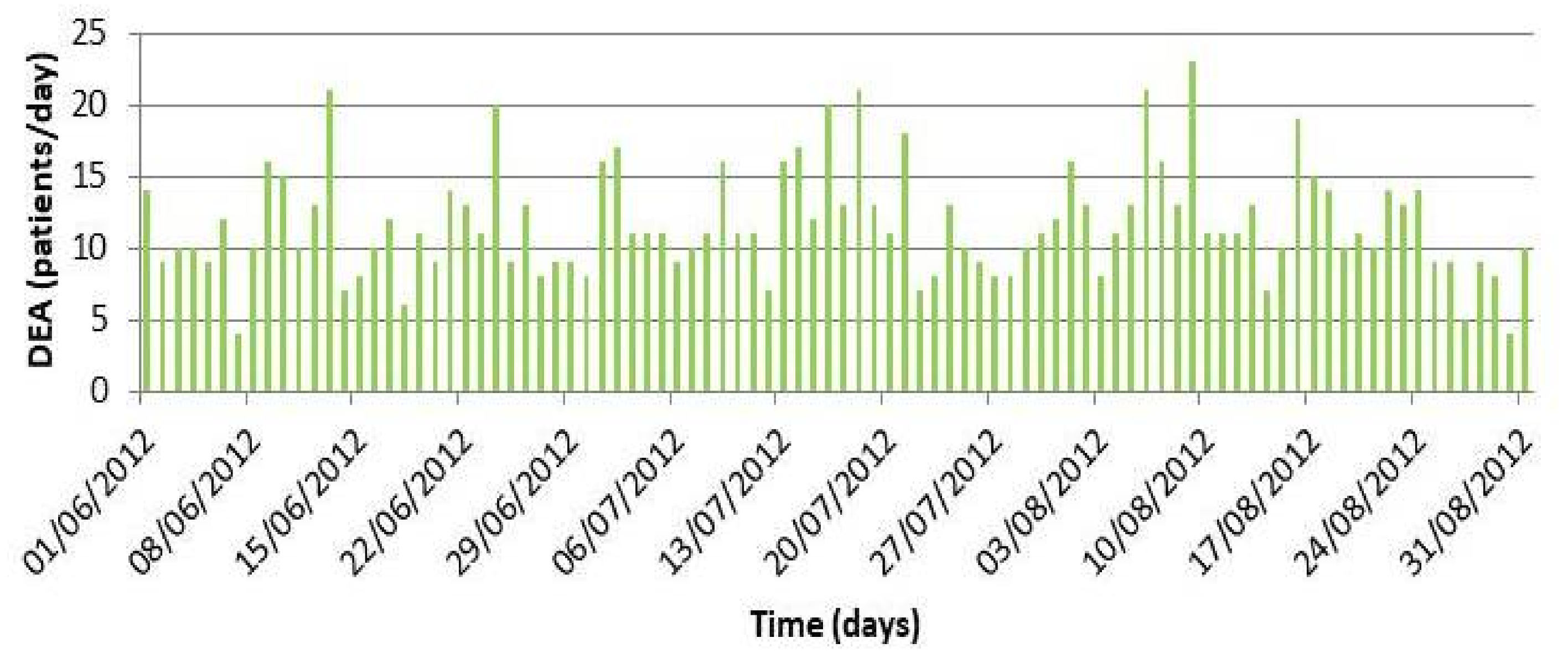
The data included admission date (day and hour), diagnostic code (International Classification of Diseases) of each admission, residence zone, age, and sex of the patient, ward type, diagnosis, and triage. The total number of patients admitted to the emergency department in the three months investigated was 7895. The heat-related illnesses analyzed in this study, usually attributed to heatstroke, were fever, headache, myalgia, dehydration, palpitations, dizziness, tachycardia, syncope, etc. The selected cases, referred to as Daily Emergency Admissions (DEA), are 1079 and represent 14% of total admissions for the Matera hospital (330 in June, 378 in July, and 371 in August). Figure 2 reports daily emergency admissions (DEA) from 1 June 2012 to 31 August 2012. The DEA data for this period show an average of 12 patients per day and a maximum value of 23 patients per day.

3. Methodology

3.1. Methodological Approach

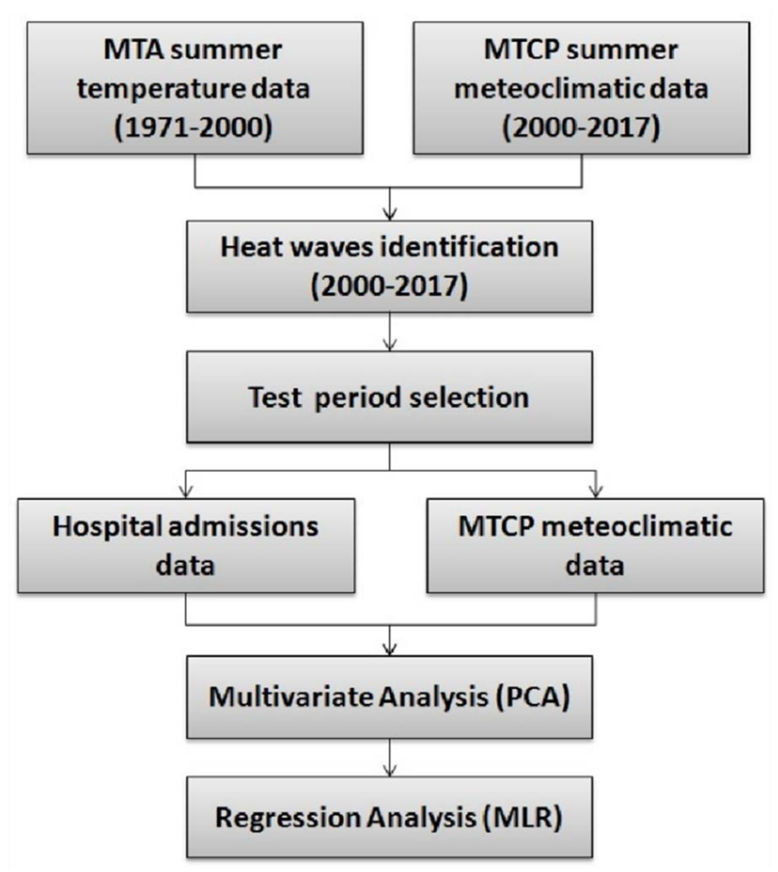
In order to better explain the methodological approach applied in this paper, in Figure 3 a block diagram is reported. It shows the main steps of the proposed analytical framework.

3.2. Temperature Analysis for the Base Period (1971–2000)

For the WMO standardized base period 1971–2000, the series of daily mean values and corresponding standard deviations were calculated as follows, starting from the summer maximum temperature $BP{T}_{ij}^{max}$ temperature (with i = 1, …, M; M = 92 days and j = 1, …, N; N = 30 years) collected at the MTA station:

$${\overline{BPT}}_i^{max}=\frac{{\sum }_{j=1}^{N}BP{T}_{ij}^{max}}{N}\mathrm{with}i=1,\dots ,M,$$

$${\sigma }_i=\sqrt{\frac{{\sum }_{j=1}^N{\left(BP{T}_{ij}^{max}-BP{T}_i^{max}\right)}^2}{N-1}}\mathrm{with}i=1,\dots ,M,.$$

(1)

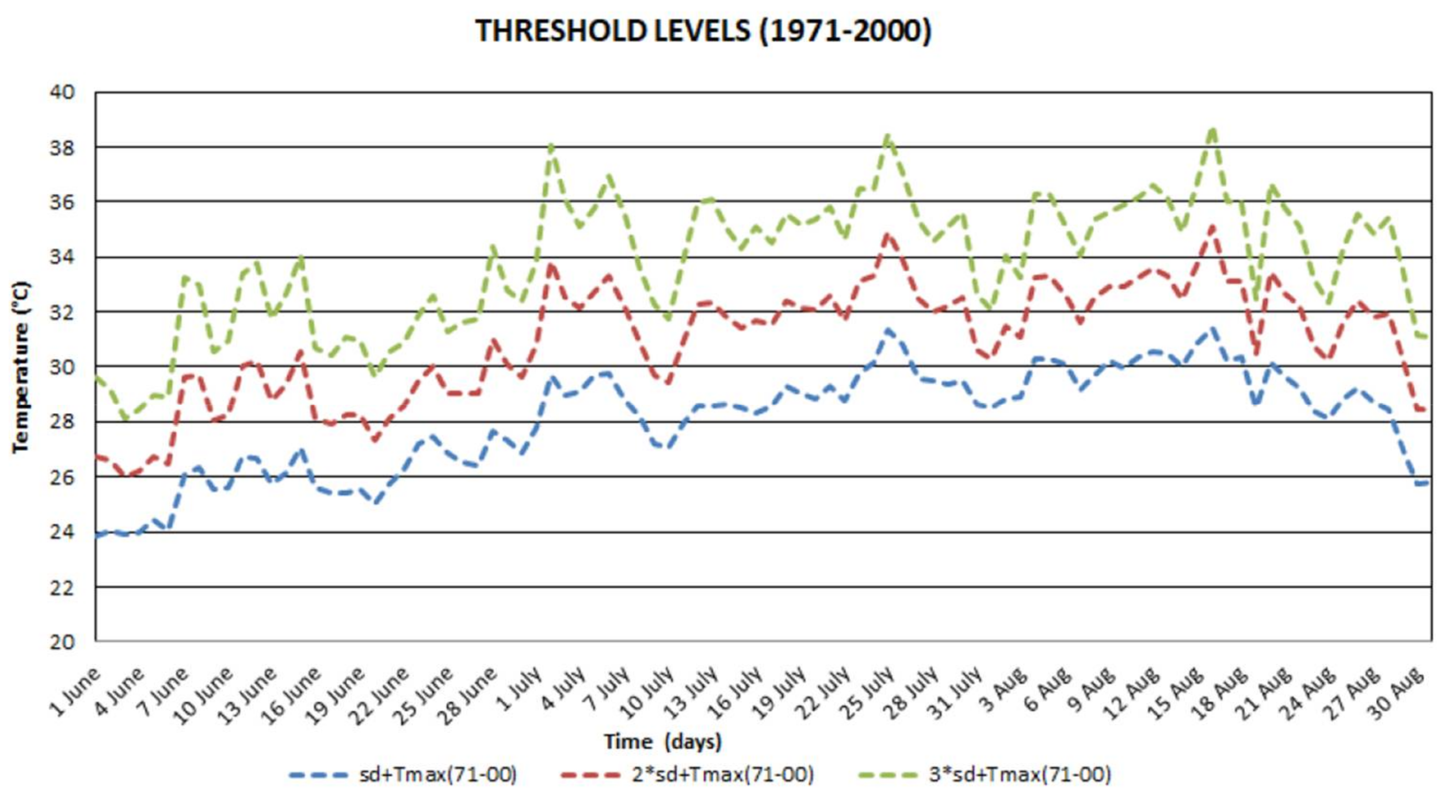
Starting from these values, three threshold series indicating an increasing level of severity with respect to the occurrence of extreme values of maximum temperature were defined:

• First threshold series:

  $$\left\{T{s}_1^I,\dots ,T{s}_M^I\right\}\mathrm{where}T{s}_i^I=\left({\overline{BPT}}_i^{max}+{\sigma }_i\right)\mathrm{with}i=1,\dots ,M,$$

  (2)
• Second threshold series:

  $$\left\{T{s}_1^{II},\dots ,T{s}_M^{II}\right\}\mathrm{where}T{s}_i^{II}=\left({\overline{BPT}}_i^{max}+2{\sigma }_i\right)\mathrm{with}i=1,\dots ,M,$$

  (3)
• Third threshold series:

  $$\left\{T{s}_1^{III},\dots ,T{s}_M^{III}\right\}\mathrm{where}T{s}_i^{III}=\left({\overline{BPT}}_i^{max}+3{\sigma }_i\right)\mathrm{with}i=1,\dots ,M.$$

  (4)

3.3. Extreme Temperature Analysis from 2000 to 2017

In order to characterize the occurrence of extreme events in maximum summer temperature data from 2000 to 2017, hot days (HDs) are defined according to the following criteria:

• the i-th summer day (i = 1, …, M) in the k-th year (k = 1, ..., N′ N′ = 18 years) is classified as a hot day of the first degree

  $$\mathit{H}{\mathit{D}}_{\mathit{L}\mathbf{1}}\mathbf{if}{\mathit{T}}_{\mathit{i}\mathit{k}}^{\mathit{m}\mathit{a}\mathit{x}}\mathbf{>}\mathit{T}{\mathit{s}}_{\mathit{i}}^{\mathit{I}}$$

  (5)
• the i-th summer day (i =1, …, M) in the k-th year (k = 1, …, N′ N′ = 18 years) is classified as a hot day of the second degree

  $$\mathit{H}{\mathit{D}}_{\mathit{L}\mathbf{2}}\mathit{if}{\mathit{T}}_{\mathit{i}\mathit{k}}^{\mathit{m}\mathit{a}\mathit{x}}\mathbf{>}\mathit{T}{\mathit{s}}_{\mathit{i}}^{\mathit{I}\mathit{I}}$$

  (6)
• the i-th summer day (i = 1, …, M) in the k-th year (k = 1, …, N′ N′ = 18 years) is classified as a hot day of the third degree

  $$\mathit{H}{\mathit{D}}_{\mathit{L}\mathbf{3}}\mathbf{if}{\mathit{T}}_{\mathit{i}\mathit{k}}^{\mathit{m}\mathit{a}\mathit{x}}\mathbf{>}\mathit{T}{\mathit{s}}_{\mathit{i}}^{\mathit{I}\mathit{I}\mathit{I}}\mathbf{.}$$

  (7)

Furthermore, to measure the persistence of these events, the occurrence of HWs was defined with the following criteria:

• occurrence of at least six consecutive days classified as

  $$\mathit{H}{\mathit{D}}_{\mathit{L}\mathbf{1}}=\mathbf{occurrence\; of\; heat\; wave\; of\; the\; first\; degree}\mathit{H}{\mathit{W}}_{\mathit{L}\mathbf{1}}$$

  (8)
• occurrence of at least six consecutive days classified as

  $$\mathit{H}{\mathit{D}}_{\mathit{L}\mathbf{2}}=\mathbf{occurrence\; of\; heat\; wave\; of\; the\; second\; degree}\mathit{H}{\mathit{W}}_{\mathit{L}\mathbf{1}}$$

  (9)
• occurrence of at least six consecutive days classified as

  $$\mathit{H}{\mathit{D}}_{\mathit{L}\mathbf{3}}=\mathbf{ccurrence\; of\; heat\; wave\; of\; the\; third\; degree}\mathit{H}{\mathit{W}}_{\mathit{L}\mathbf{3}}.$$

  (10)

For each HW, the corresponding length or determined intensity (as the number of consecutive days in which a HD occurred) was also reported.

3.4. Correlation Analysis of Weather Conditions and Daily Emergency Admissions

To investigate the correlation structure between weather data and daily emergency admissions (number of daily cases), a Principal Component Analysis (PCA) technique and a Multiple Linear Regression (MLR) model were applied [37,43,44,45,46].

To apply PCA, minimum and maximum daily temperatures ($T^{min}$ and $T^{max}$), minimum and maximum daily relative humidity ($R{H}^{min}$ and $R{H}^{max}$), daily barometric pressure range ($DPR$), and daily emergency admissions (DEA) were organized in an input matrix (6 descriptors × 92 summer days). In this case, the approach made it possible to highlight the underlying correlation pattern among the six descriptors. Moreover, a Multiple Linear Regression analysis was performed. In particular, MLR generalizes the prediction methodology to allow for multiple weather predict variables. The MLR model used was:

Y = β₀ + β₁w₁ + β₂w₂ + …… + β_nw_n

(11)

where, Y, Dependent variable = DEA; β₀, Constant; β_(1–6), Unstandardized coefficient for each predictor weather variable; w₁ to w_n, Predictor weather variables.

4. Results and Discussion

Regarding data analysis of temperature in the base period, the three threshold series used to identify extreme events of summer maximum temperature are presented in Figure 4. The use of an extension of the 3σ-rule allows us to take into account statistically significant events in terms of frequency occurrence in the range 0.68–0.99.

Comparing these series with data measured in summers from 2000 to 2017, the HDs and HWs occurring in these years were counted and are summarized in

Table 1. Number of hot days (HDs) with the corresponding percentage calculated on all summer days (M = 92).

Year	$\mathit{n}(\mathit{H}{\mathit{D}}_{\mathit{L}1})$	$\mathit{n}(\mathit{H}{\mathit{D}}_{\mathit{L}2})$	$\mathit{n}(\mathit{H}{\mathit{D}}_{\mathit{L}3})$
2000	70 (76%)	42 (46%)	25 (27%)
2001	77 (84%)	42 (46%)	14 (15%)
2002	92 (100%)	38 (41%)	0 (0%)
2003	89 (97%)	65 (71%)	46 (50%)
2004	68 (74%)	45 (49%)	20 (22%)
2005	68 (74%)	45 (49%)	27 (29%)
2006	55 (60%)	32 (35%)	23 (25%)
2007	74 (80%)	58 (63%)	32 (35%)
2008	78 (85%)	48 (52%)	28 (30%)
2009	69 (75%)	41 (45%)	15 (16%)
2010	68 (74%)	45 (49%)	18 (20%)
2011	74 (80%)	49 (53%)	25 (27%)
2012	84 (91%)	74 (80%)	49 (53%)
2013	65 (71%)	35 (38%)	16 (17%)
2014	59 (64%)	30 (33%)	8 (9%)
2015	75 (81%)	51 (55%)	25 (27%)
2016	66 (72%)	39 (42%)	14 (15%)
2017	76 (83%)	65 (71%)	38 (41%)

In bold are the cases in which the percentage of HDs for the three levels is greater than 90%, 70%, and 50%, respectively.

and

Table 2. Number of heat waves (HW) with the corresponding intensities expressed in number of days.

Year	$\mathit{n}(\mathit{H}{\mathit{W}}_{\mathit{L}1})$	$\mathit{n}(\mathit{H}{\mathit{W}}_{\mathit{L}2})$	$\mathit{n}(\mathit{H}{\mathit{W}}_{\mathit{L}3})$
2000	5 (9, 7, 15, 8, 21)	1 (9)	1 (7)
2001	5 (10, 15, 20, 7, 9)	1 (11)	0
2002	1 (92)	1 (13)	0
2003	2 (61, 24)	3 (14, 11, 15)	2 (11, 11)
2004	4 (8, 25, 10, 7)	1 (16)	0
2005	5 (7, 19, 7, 20, 7)	3 (15, 8, 8)	2 (10, 7)
2006	4 (18, 7, 10, 10)	1 (16)	1 (15)
2007	3 (25, 17, 19)	2 (22, 11)	2 (12, 8)
2008	4 (30, 15, 7, 13)	2 (16, 10)	0
2009	3 (17, 8, 12)	1 (8)	0
2010	3 (16, 16, 19)	2 (9, 14)	0
2011	4 (10, 16, 11, 20)	3 (9, 13, 15)	0
2012	3 (46, 16, 14)	4 (9, 31, 13, 8)	2 (11, 8)
2013	4 (12, 7, 23, 9)	2 (11, 8)	1 (8)
2014	4 (11, 7, 8, 12)	0	0
2015	3 (17, 40, 9)	1 (22)	1 (7)
2016	2 (25, 11)	1 (7)	0
2017	6 (7, 13, 11, 8, 15, 9)	4 (7, 12, 8, 13)	2 (7, 12)

In bold, the cases in which the greatest number of extreme events occurred.

. For each year, the number of HDs according to the different levels of severity is specified in Table 1.

The number of HWs for each year, with corresponding intensities (expressed in number of days) according to the different levels of severity, are listed in Table 2.

It is possible to note that the highest number of HDs occurred in 2002, 2003, 2012, and 2017, while the highest HW_L3 (combining number of events and intensity) was recorded in 2003 and 2012. Furthermore, Table 1 and Table 2 reveal two years with atypical cases: in 2002, there was a maximum number of HD_L1 (92 days) but no HW_L3; on the contrary, 2007 presented a low number of HDs and two extreme events with high intensity.

Therefore, we can say that three levels for HW classification made it possible to point out years characterized by a high percentage of HDs which do not necessarily determine situations of extreme severity at higher levels of HWs, especially in the third level.

Year 2012 was chosen to investigate a specific case among the four years in which there was an occurrence of HW_L3. In fact, for this year data were available from the public system of “Madonna delle Grazie” Hospital.

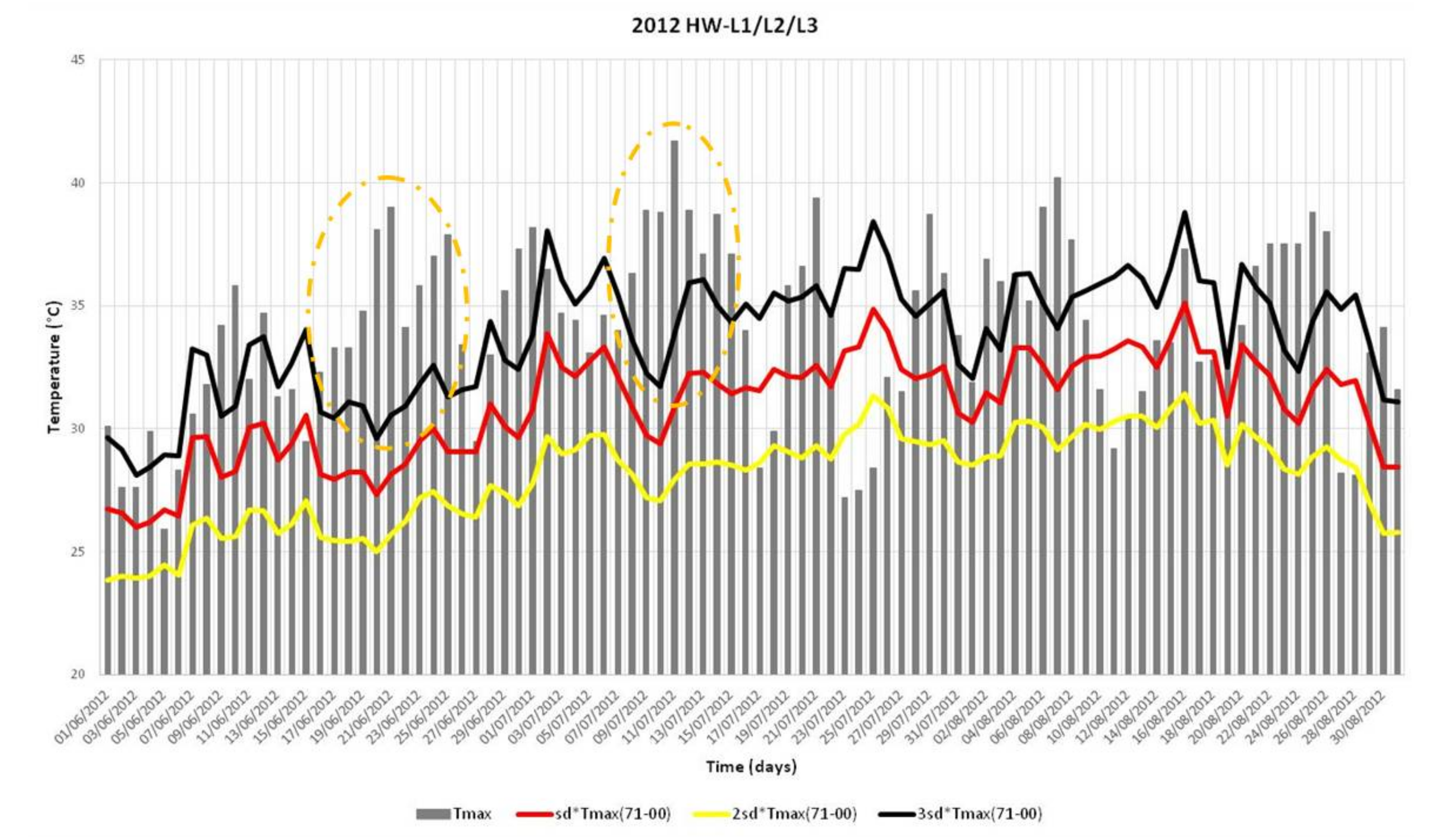
The pattern of maximum temperatures in the summer of 2012 is compared in Figure 5 with the three threshold series to put in evidence the periods in which the extreme events occurred.

In particular, for each HW, it is possible to identify:

Three HW_L1: from 1 June to 16 July (46 days); from 27 July to 10 August (15 days); and from 13 August to 26 August, (19 days).

Four HW_L2: from 6 June to 14 June (9 days) and from 16 June to 16 July (31 days) included in the first HW_L1; from 28 July to 9 August (13 days) included in the second HW_L1; and from 19 August to 26 August (8 days) included in the third HW_L1.

Two HW_L3: from 16 June to 26 June (11 days) and from 8 July to 15 July (8 days) included both in the second HW_L2 (Figure 5).

To investigate the correlation structure among weather conditions and DEA data in summer 2012, PCA was applied. All data (with no data missing) were organized in an input matrix [6 descriptors × 92 summer days].

Table 3. Explorative statistical analysis of meteo-climatic database.

Variable	Units	min	max	m	sd
Tmax	(°C)	25.9	41.7	34.1	3.5
Tmin	(°C)	14.8	28.6	23.0	3.1
DPR	(hPa)	1.0	7.0	2.6	1.1
RHmax	(%)	37.0	100.0	68.0	19.0
RHmin	(%)	14.0	56.0	28.0	9.0
DEA	(n/day)	4.00	23.00	11.73	3.9

Legend: m = mean value; sd = standard deviation; DPR = daily barometric pressure range; RH = relative humidity.

summarizes the descriptive statistics.

The results of PCA are shown in

Table 4. PCA results.

	F1	F2	F3
λi	3.16	1.14	1.00
P(λi)	52.7%	19.0%	13.4%
Ptot		71.7%	85.1%
	F1	F2	F3
Tmax	27%	-	-
Tmin	24%	-	-
DPR	-	54%	35%
RHmax	21%	-	6%
RHmin	22%	-	13%
DEA	-	44%	44%

Legend: λ_i = eigenvalue; P(λ_i) = percentage of variance explained by i-th eigenvalue; P_tot = cumulative percentage of variance; A_i = i-th eigenvector.

. Combining the Kaiser’s rule for the selection of significant eigenvalues and the empiric rule for the factor characterization (loadings >0.71 are regarded as excellent and <0.32 as very poor), only eigenvalues higher than 1 and loadings higher than 0.4 were taken into account [47,48]. In this investigated case, the first three eigenvalues explained 85% of the data variance. To interpret these three principal components (PCs), only the percentage contributions of original descriptors higher than 5% were considered (Table 4).

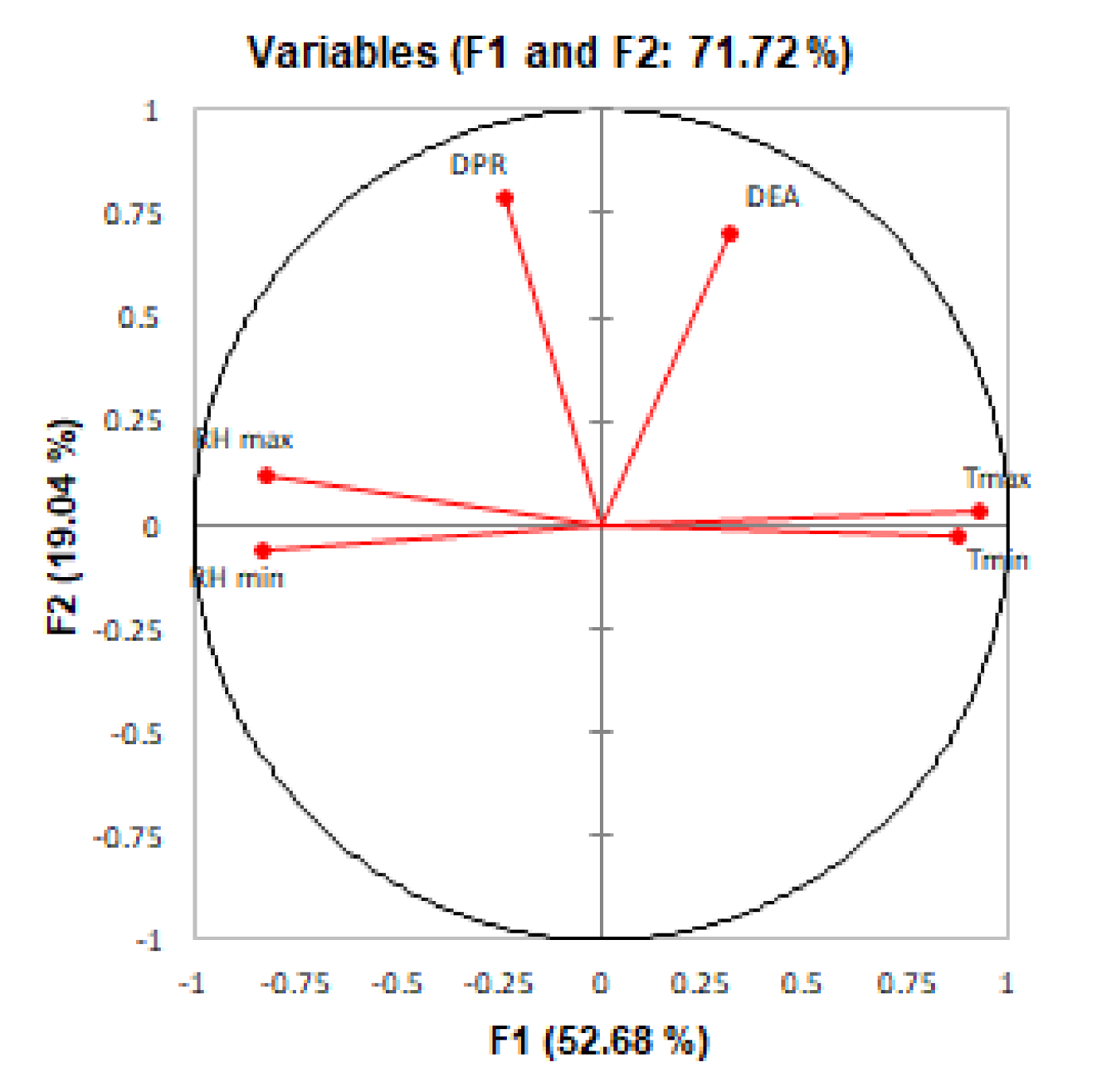
It was possible to identify three new variables: the first variable is represented by a linear combination of T^max, T^min, RH^max, and RH^min (the percentage of explained variance was 52.7%); the second by a linear combination of DPR and DEA (the percentage of explained variance was 19%); and the third includes DPR, DEA, RH^max, and RH^min (explaining 13.4% of variance). In Figure 6, the original descriptors are shown in the principal component system: temperatures and relative humidity have opposite signs while temperatures and DEA data appear in the same quadrant.

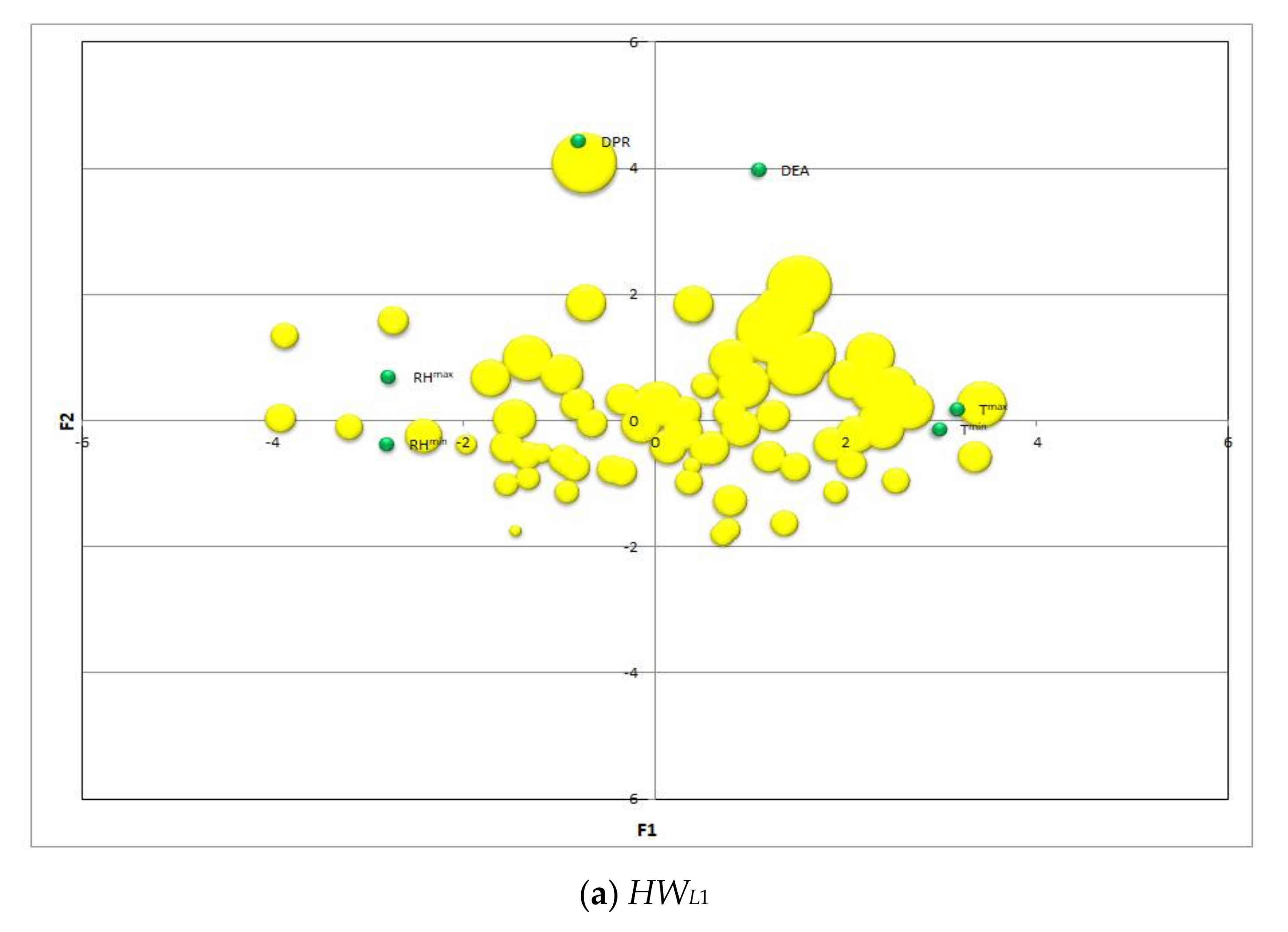
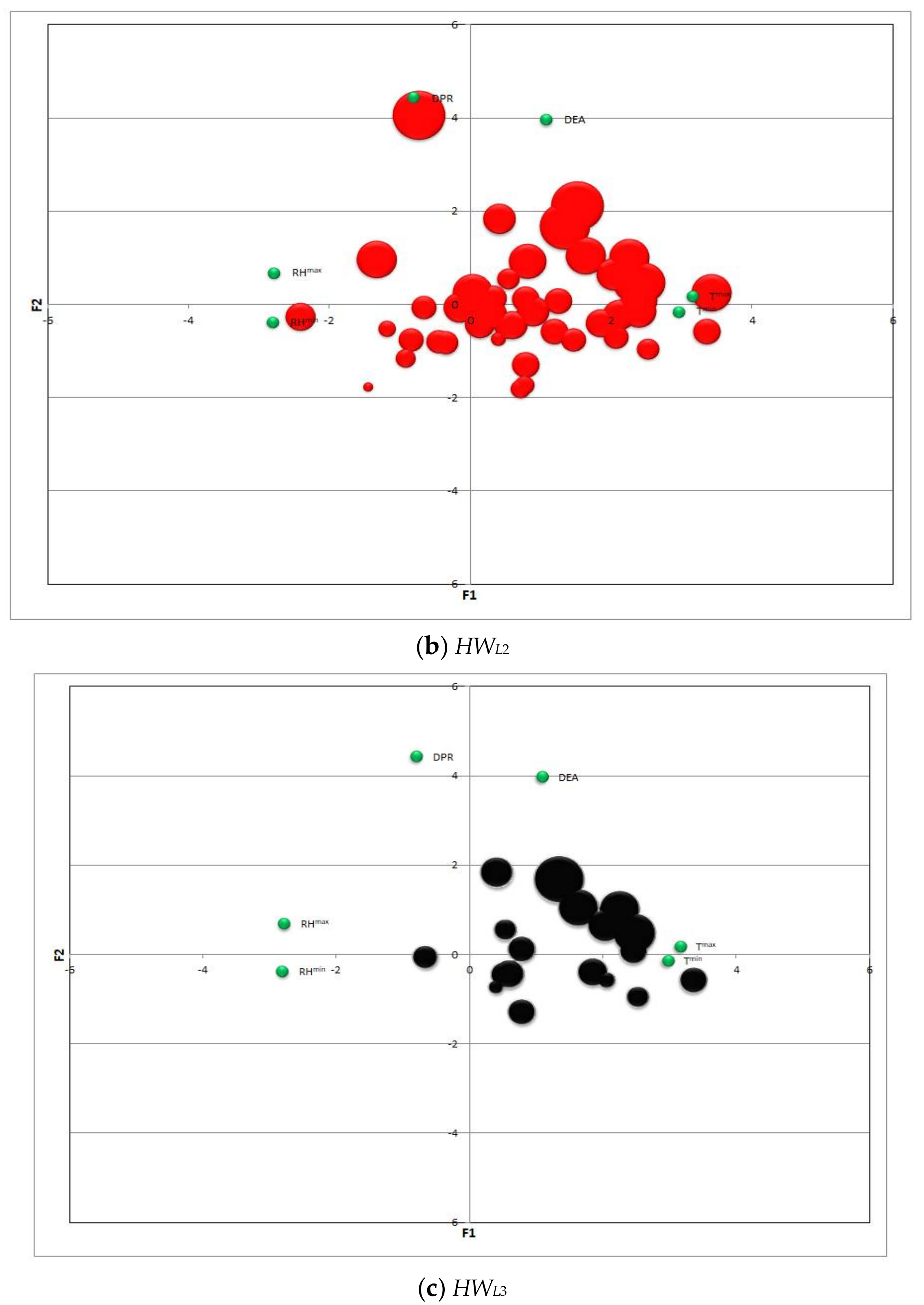
PCA allowed for the reduction of the set of weather descriptors. In particular, the six original variables were separated into two different sets (T^max, T^min, RH^max, RH^min) and (DPR, DEA). To improve interpretation of the correlation structure, it is interesting to associate PCA results and HD identification. In the three score plots (F₁ versus F₂) depicted in Figure 7, the size of bubbles is proportional to the corresponding DEA value. It is possible to note that from threshold level 1 to level 3, the size of bubbles tends to increase. These results highlight the increase in severity level of HDs, decreasing the role of relative humidity. For the maximum level of threshold (HW_L3), the correlation between DEA and HWs is linked to a combination of DPR and temperatures.

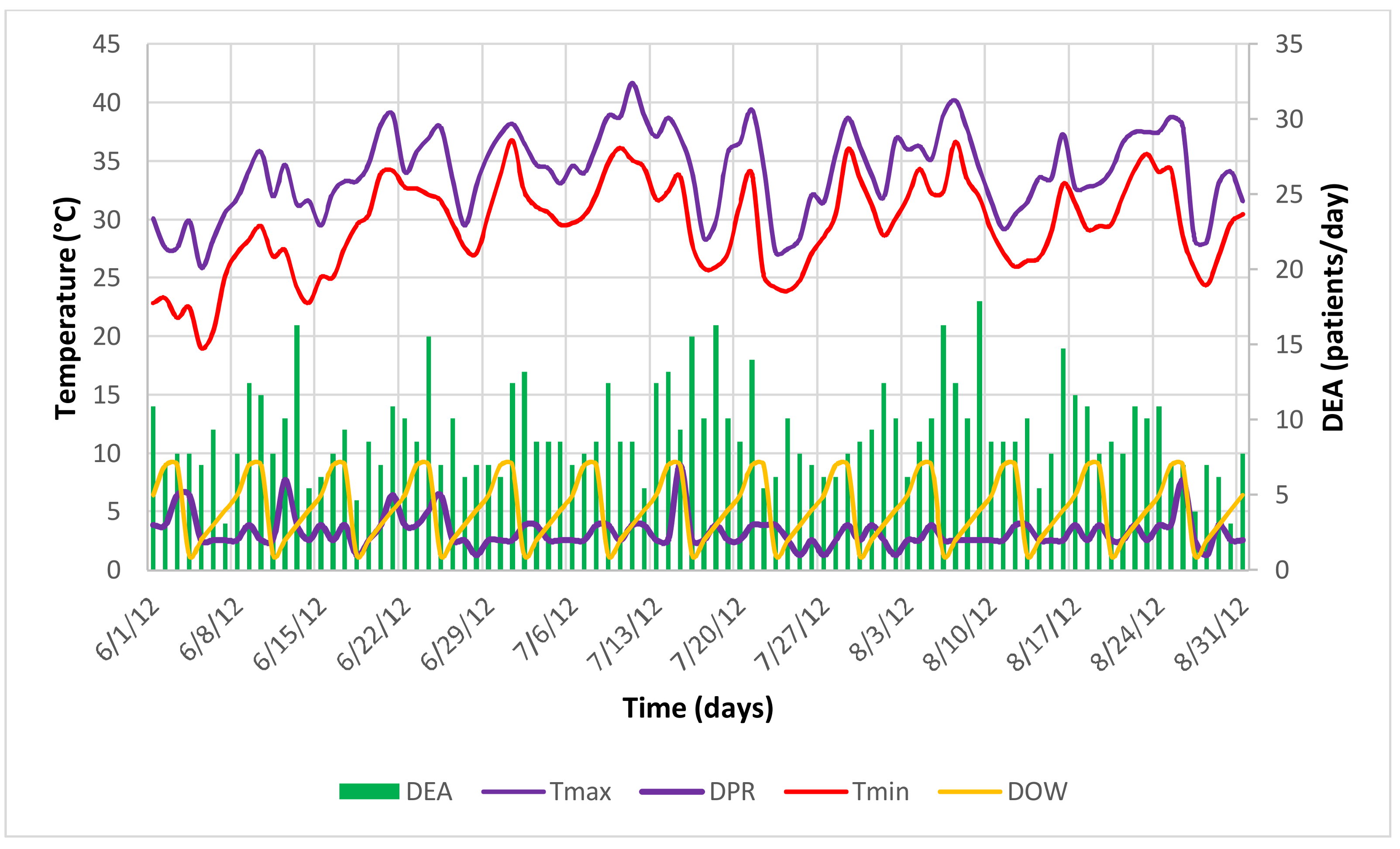
In order to analyze the relationship between DEA values and weather variables in summer 2012 and according to multivariate statistical analysis, a multiple linear regression model was developed. In this context, the following variables were considered: ln(DEA) (natural logarithm of Daily Emergency Admissions), T^max, T^min, and DPR. To take into account the influence of holidays (including Saturdays) in daily admission in the emergency room, the DOW (day of week) variable was also considered (Figure 8).

Furthermore, an autocorrelation test of temperatures and DPR data series was carried out, allowing for consideration of the two-day lagged series in the regression model. The multiple linear regression model parameters are reported in

Table 5. Multiple Linear Regression model parameters.

Variables	Coefficient	t Statistics
Intercept	1.472	14.023
X1 Tmax(lag2)	0.018	3.323
X2 Tmin(lag2)	0.016	3.126
X3 DPR(lag2)	0.014	2.890
X4 DOW	0.002	2.616

.

In particular, the parameter values reported in Table 5 show the marginal role of DOW in the process (β = 0.002, p < 0.01). On the contrary, the effect of temperature (maximum and minimum) and DPR(lag₂) is greater (β = 0.018 and p < 0.001, β = 0.016 and p < 0.001, β = 0.014 and p < 0.001, respectively), representing DEA precursors and consequently of potential use in surveillance of hospital admission risk factors.

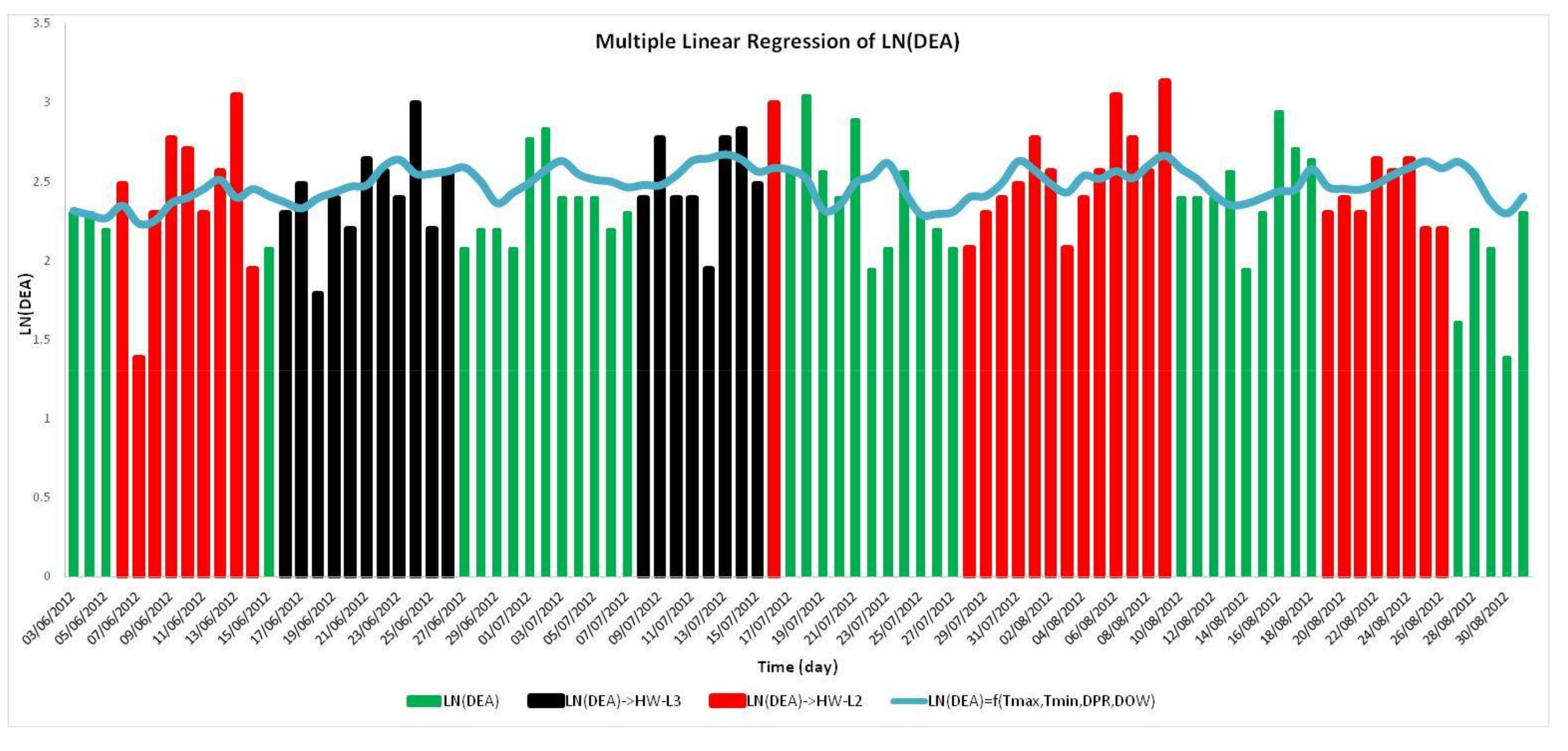
Figure 9 shows the trend of DEA for high threshold levels (HW_L2 and HW_L3) and the obtained multiple linear regression model. From the figure, it is possible to observe that even if the model is unable to reproduce DEA (R²adj = 0.33) peak values (probably due to the short observation period), the model estimates the DEA trend very well for nearly the entire period of analysis and for each HW threshold level. This confirms the results obtained also by multivariate analysis, which indicate that, especially for extreme events (HW_L2 and HW_L3), the DEA was strongly related to temperatures (maximum and minimum) and DPR.

5. Conclusions

Based on common scientific knowledge, under which temporal weather variations have an impact on satisfaction with life (in particular on individuals with poor health condition), this study assessed the impact of high temperatures, typically related to heat waves, on daily hospital admissions between 1 June 2012 and 31 August 2012 at the emergency room of a hospital in Matera, Italy. In particular, a methodology composed of several methods was applied: a procedure to identify the heat waves in a 2000–2017 dataset compared to the base period (1970–1999) and, subsequently, a PCA technique and MLR model to examine the association between DEA and weather data for summer 2012.

The analysis of daily mean values and standard deviations of maximum temperatures in the 2000–2017 period made it possible to detect three threshold series, which reflect the occurrence of HWs. The years 2003, 2012, and 2017 presented the maximum frequency of hot days and heat waves (with a third-level HW-days percentage greater than 20%). In 2012, HW_L3 occurred between the third and fourth weeks of June and the first two weeks of July.

The results of PCA show that the role of relative humidity decreases when the severity level of HWs increases. Moreover, the results of the PCA and MLR model highlight the combination of temperatures (T^max and T^min) and DPR as precursors for a surveillance system of risk factors in hospital admissions.

The paper first highlights some important strengths of the methodology as the total replicability in other similar contexts. On the contrary, the weakness point of this work is the length of the available dataset, which did not allow for a verification of the predictive capabilities of the model. For these reasons, future developments will address the prediction of the values of DEA (e.g., analysis of a dataset that also includes the 2017 year in order to verify the predictive capabilities of the model) and the development of other techniques both for the identification of the heatwaves (anomalies detection) and for the predictive model (machine learning).

References

- Phung, D.; Guo, Y.; Thai, P.; Rutherford, S.; Wang, X.; Nguyen, M.; Manh Do, C.; Huy Nguyen, N.; Alam, N.; Chu, C. The effects of high temperature on cardiovascular admissions in the most populous tropical city in Vietnam. Environ. Pollut. 2016, 208, 33–39. [Google Scholar] [CrossRef] [PubMed]
- Noelke, C.; McGovern, M.; Corsi, D.J.; Jimenez, M.P.; Stern, A.; Wing, I.S.; Berkman, L. Increasing ambient temperature reduces emotional well-being. Environ. Res. 2016, 151, 124–129. [Google Scholar] [CrossRef] [PubMed]
- Barrington-Leigh, C.; Behzadnejad, F. The impact of daily weather conditions on life satisfaction: Evidence from cross-sectional and panel data. J. Econ. Psychol. 2017, 59, 145–163. [Google Scholar] [CrossRef]
- Lee, W.V. Historical global analysis of occurrences and human casualty of extreme temperature events (ETEs). Nat. Hazards 2014, 70, 1453–1505. [Google Scholar] [CrossRef]
- Wilbanks, T.J.; Fernandez, S.J.; Allen, M.R. Extreme weather events and interconnected infrastructures: Toward more comprehensive climate change planning. Environment 2015, 57, 4–15. [Google Scholar] [CrossRef]
- Cioffi, F.; Conticello, F.; Lall, U.; Marotta, L.; Telesca, V. Large scale climate and rainfall seasonality in a Mediterranean Area: Insights from a non-homogeneous Markov model applied to the Agro-Pontino plain. Hydrol. Processes 2017, 31, 668–686. [Google Scholar] [CrossRef]
- Elferchichi, A.; Giorgio, G.A.; Lamaddalena, N.; Ragosta, M.; Telesca, V. Variability of temperature and its impact on reference evapotranspiration: The test case of the Apulia Region (Southern Italy). Sustainability 2017, 9, 2337. [Google Scholar] [CrossRef]
- Connolly, M. Some like it mild and not too wet: The influence of weather on subjective well-being. J. Happiness Stud. 2013, 14, 457–473. [Google Scholar] [CrossRef]
- Denissen, J.J.; Butalid, L.; Penke, L.; Van Aken, M.A. The effects of weather on daily mood: A multilevel approach. Emotion 2008, 8, 662. [Google Scholar] [CrossRef] [PubMed]
- Lucas, R.E.; Lawless, N.M. Does life seem better on a sunny day? Examining the association between daily weather conditions and life satisfaction judgments. J. Pers. Soc. Psychol. 2013, 104, 872. [Google Scholar] [CrossRef] [PubMed]
- Basagaña, X.; Sartini, C.; Barrera-Gómez, J.; Dadvand, P.; Cunillera, J.; Ostro, B.; Sunyer, J.; Medina-Ramón, M. Heat waves and cause-specific mortality at all ages. Epidemiology 2011, 22, 765–772. [Google Scholar] [CrossRef] [PubMed]
- Kim, Y.; Kim, H.; Honda, Y.; Guo, Y.L.; Chen, B.Y.; Woo, J.M.; Ebi, K.L. Suicide and ambient temperature in East Asian countries: A time-stratified case-crossover analysis. Environ. Health Perspect. 2016, 124, 75. [Google Scholar] [CrossRef] [PubMed]
- Qi, X.; Hu, W.; Page, A.; Tong, S. Associations between climate variability, unemployment and suicide in Australia: A multicity study. BMC Psychiatry 2015, 15, 114. [Google Scholar] [CrossRef] [PubMed]
- Zuo, J.; Pullen, S.; Palmer, J.; Bennetts, H.; Chileshe, N.; Ma, T. Impacts of heat waves and corresponding measures: A review. J. Clean. Prod. 2015, 92, 1–12. [Google Scholar] [CrossRef]
- Huntington, T.G. Evidence for intensification of the global water cycle: Review and synthesis. J. Hydrol. 2006, 319, 83–95. [Google Scholar] [CrossRef]
- Arbuthnott, K.G.; Hajat, S. The health effects of hotter summers and heat waves in the population of the United Kingdom: A review of the evidence. Environ. Health 2017, 16, 119. [Google Scholar] [CrossRef] [PubMed]
- Zittis, G.; Hadjinicolaou, P.; Fnais, M.; Lelieveld, J. Projected changes in heat wave characteristics in the eastern Mediterranean and the Middle East. Reg. Environ. Chang. 2016, 16, 1863–1876. [Google Scholar] [CrossRef]
- Giorgio, G.A.; Ragosta, M.; Telesca, V. Climate variability and industrial-suburban heat environment in a Mediterranean area. Sustainability 2017, 9, 775. [Google Scholar] [CrossRef]
- Crimmins, A.; Balbus, J.; Gamble, J.L.; Beard, C.B.; Bell, J.E.; Dodgen, D.; Eisen, R.J.; Fann, N.; Hawkins, M.D.; Herring, S.C.; et al. The Impacts of Climate Change on Human Health in the United States: A Scientific Assessment; U.S. Global Change Research Program: Washington, DC, USA, 2016; p. 321. Available online: https://health2016.globalchange.gov/downloads (accessed on 10 February 2018).
- Morabito, M.; Crisci, A.; Messeri, A.; Messeri, G.; Betti, G.; Orlandini, S.; Raschi, A.; Maracchi, G. Increasing heatwave hazards in the southeastern European Union capitals. Atmosphere 2017, 8, 115. [Google Scholar] [CrossRef]
- Williams, S.; Nitschke, M.; Weinstein, P.; Pisaniello, D.L.; Parton, K.A.; Bi, P. The impact of summer temperatures and heatwaves on mortality and morbidity in Perth, Australia 1994–2008. Environ. Int. 2012, 40, 33–38. [Google Scholar] [CrossRef] [PubMed]
- Wang, X.Y.; Barnett, A.G.; Yu, W.; FitzGerald, G.; Tippett, V.; Aitken, P.; Neville, G.; McRae, D.; Verrall, K.; Tong, S. The impact of heatwaves on mortality and emergency hospital admissions from non-external causes in Brisbane, Australia. Occup. Environ. Med. 2012, 69, 163–169. [Google Scholar] [CrossRef] [PubMed]
- García-Herrera, R.; Díaz, J.; Trigo, R.M.; Luterbacher, J.; Fischer, E.M. A review of the European summer heat wave of 2003. Crit. Rev. Environ. Sci. Technol. 2010, 40, 267–306. [Google Scholar] [CrossRef]
- Tolika, K.; Maheras, P.; Tegoulias, I. Extreme temperatures in Greece during 2007: Could this be a “return to the future”? Impact of historical land use and soil management change on soil erosion and agricultural sustainability during the Anthropocene. Anthropocene 2009, 17, 13–29. [Google Scholar]
- Rebetez, M.; Dupont, O.; Giroud, M. An analysis of the July 2006 heatwave extent in Europe compared to the record year of 2003. Theor. Appl. Climatol. 2009, 95, 1–7. [Google Scholar] [CrossRef]
- Barriopedro, D.; Fischer, E.M.; Luterbacher, J.; Trigo, R.M.; García-Herrera, R. The hot summer of 2010: Redrawing the temperature record map of Europe. Science 2011, 332, 220–224. [Google Scholar] [CrossRef] [PubMed]
- Green, H.K.; Andrews, N.; Armstrong, B.; Bickler, G.; Pebody, R. Mortality during the 2013 heatwave in England—How did it compare to previous heatwaves? A retrospective observational study. Environ. Res. 2016, 147, 343–349. [Google Scholar] [CrossRef] [PubMed]
- Telesca, V.; Lay-Ekuakille, A.; Ragosta, M.; Giorgio, G.A.; Lumpungu, B. Monitoring of extreme temperatures to evaluate the interaction between climate change and human health in coastal areas. In Proceedings of the 6th EnvImeko—IMEKO TC19 Symposium on Environmental Instrumentation and Measurements, Reggio Calabria, Italy, 24–25 June 2016; p. 95, ISBN 978-1-5108-2812-4. [Google Scholar]
- D’Ippoliti, D.; Michelozzi, P.; Marino, C.; de’Donato, F.; Menne, B.; Katsouyanni, K.; Kirchmayer, U.; Analitis, A.; Medina-Ramon, M.; Paldy, A.; et al. The impact of heat waves on mortality in 9 European cities: Results from the EuroHEAT project. Environ. Health 2010, 9, 37. [Google Scholar] [CrossRef] [PubMed]
- Michelozzi, P.; Accetta, G.; De Sario, M.; D’Ippoliti, D.; Marino, C.; Baccini, M.; Biggeri, A.; Anderson, H.R.; Katsouyanni, K.; Ballester, F.; et al. High temperature and hospitalizations for cardiovascular and respiratory causes in 12 European cities. Am. J. Respir. Crit. Care Med. 2009, 179, 383–389. [Google Scholar] [CrossRef] [PubMed]
- McGregor, G.R.; Bessemoulin, P.; Ebi, K.; Menne, B. (Eds.) Heat Waves and Health: Guidance on Warning System Development. Report to the World Meteorological Organization and World Health Organization; World Meteorological Organization: Geneva, Switzerland, 2015; Available online: http://www.who.int/globalchange/publications/heatwaves-health-guidance/en (accessed on 10 February 2018).
- Sánchez, J.M.; Scavone, G.; Caselles, V.; Valor, E.; Copertino, V.A.; Telesca, V. Monitoring daily evapotranspiration at a regional scale from Landsat-TM and ETM+ data: Application to the Basilicata region. J. Hydrol. 2008, 351, 58–70. [Google Scholar] [CrossRef]
- Copertino, V.A.; Di Pierro, M.; Scavone, G.; Telesca, V. Comparison of algorithms to retrieve Land Surface Temperature from LANDSAT-7 ETM+ IR data in the Basilicata Ionian band. Tethys J. Weather Clim. West. Mediterr. 2012, 9, 25–34. [Google Scholar] [CrossRef]
- Scavone, G.; Sánchez, J.M.; Telesca, V.; Caselles, V.; Copertino, V.A.; Pastore, V.; Valor, E. Pixel-oriented land use classification in energy balance modelling. Hydrol. Processes 2014, 28, 25–36. [Google Scholar] [CrossRef]
- Blasi, M.G.; Liuzzi, G.; Masiello, G.; Serio, C.; Telesca, V.; Venafra, S. Surface parameters from SEVIRI observations through a Kalman filter approach: Application and evaluation of the scheme to the southern Italy. Tethys J. Weather Clim. West. Mediterr. 2016, 13, 3–10. [Google Scholar] [CrossRef]
- Buscail, C.; Upegui, E.; Viel, J.F. Mapping heatwave health risk at the community level for public health action. Int. J. Health Geogr. 2012, 11, 38. [Google Scholar] [CrossRef] [PubMed] [Green Version]
- Giorgio, G.A.; Ragosta, M.; Telesca, V. Application of a multivariate statistical index on series of weather measurements at local scale. Measurement 2017, 112, 61–66. [Google Scholar] [CrossRef]
- Lay-Ekuakille, A.; Telesca, V.; Ragosta, M.; Giorgio, G.A.; Mvemba, P.K.; Kidiamboko, S. Supervised and Characterized Smart Monitoring Network for Sensing Environmental Quantities. IEEE Sens. J. 2017, 17, 7812–7819. [Google Scholar] [CrossRef]
- Field, C.B.; Barros, V.; Stocker, T.F.; Qin, D.; Dokken, D.; Ebi, K.L.; Mastrandrea, M.D.; Mach, K.J.; Plattner, G.K.; Allen, S.K. (Eds.) Managing the Risks of Extreme Events and Disasters to Advance Climate Change Adaptation; A Special Report of Working Groups I and II of the Intergovernmental Panel on Climate Change (IPCC); Cambridge University Press: Cambridge, UK, 2012; p. 582. [Google Scholar]
- Beniston, M.; Stephenson, D.B.; Christensen, O.B.; Ferro, C.A.; Frei, C.; Goyette, S.; Halsnaes, K.; Holt, T.; Jylhä, K.; Koffi, B.; et al. Future extreme events in European climate: An exploration of regional climate model projections. Clim. Chang. 2007, 81, 71–95. [Google Scholar] [CrossRef]
- Ragosta, M.; Caggiano, R.; D’Emilio, M.; Macchiato, M. Source origin and parameters influencing levels of heavy metals in TSP, in an industrial background area of Southern Italy. Atmos. Environ. 2002, 36, 3071–3087. [Google Scholar] [CrossRef]
- Caggiano, R.; Sabia, S.; D’Emilio, M.; Macchiato, M.; Anastasio, A.; Ragosta, M.; Paino, S. Metal levels in fodder, milk, dairy products, and tissues sampled in ovine farms of Southern Italy. Environ. Res. 2005, 99, 48–57. [Google Scholar] [CrossRef] [PubMed]
- Di Leo, S.; Cosmi, C.; Ragosta, M. An application of multivariate statistical techniques to partial equilibrium models outputs: The analysis of the NEEDS-TIMES Pan European model results. Renew. Sustain. Energy Rev. 2015, 49, 108–120. [Google Scholar] [CrossRef]
- Amegah, A.K.; Rezza, G.; Jaakkola, J.J. Temperature-related morbidity and mortality in Sub-Saharan Africa: A systematic review of the empirical evidence. Environ. Int. 2016, 91, 133–149. [Google Scholar] [CrossRef] [PubMed]
- Hatvani-Kovacs, G.; Belusko, M.; Pockett, J.; Boland, J. Can the excess heat factor indicate heatwave-related morbidity? A case study in Adelaide, South Australia. EcoHealth 2016, 13, 100–110. [Google Scholar] [CrossRef] [PubMed]
- Chan, E.Y.Y.; Huang, Z.; Mark, C.K.M.; Guo, C. Weather information acquisition and health significance during extreme cold weather in a subtropical city: A cross-sectional survey in Hong Kong. Int. J. Disaster Risk Sci. 2017, 8, 134–144. [Google Scholar] [CrossRef]
- Reio, T. G., Jr.; Shuck, B. Exploratory factor analysis: Implications for theory, research, and practice. Adv. Dev. Hum. Resour. 2015, 17, 12–25. [Google Scholar] [CrossRef]
- Han, Y.M.; Cao, J.J.; Jin, Z.D.; An, Z.S. Elemental composition of aerosols in Daihai, a rural area in the front boundary of the summer Asian monsoon. Atmos. Res. 2009, 92, 229–235. [Google Scholar] [CrossRef]
Figure 1.
Meteorological stations in Matera (MaTera Alsia station in the upper left corner; MaTera Civil Protection station in the lower left corner; Matera orthophoto in the lower right corner; Basilicata region localization in upper right.
Figure 2.
Daily emergency admissions (DEA) trend in summer 2012.
Figure 3.
Flow chart of the methodological approach. MTA: Matera Alsia; MTCP: Matera Civil Protection; PCA: principal component analysis; MLR: multiple linear regression.
Figure 4.
Maximum temperature threshold levels (base period 1971–2000).
Figure 5.
Trend of maximum temperatures of summer 2012 compared with the three threshold series of HW.
Figure 6.
Correlations between variables and factors.
Figure 7.
Bubble chart with correlations of DEA and meteo-climatic variables, on the principal components, for the three threshold levels.
Figure 8.
Trend of DOW (day of week) variable compared to temperatures, DPR, and DEA.
Figure 9.
Trend of DEA for HWL2 and HWL3 threshold levels and the multiple regression model result.