The Spatial and Temporal Research on the Coupling and Coordinated Relationship between Social Economy and Energy Environment in the Belt and Road Initiatives

Abstract

The Belt and Road Initiative (BRI) was presented by China’s central government to achieve regional economic cooperation under the background of economic globalization. Energy and environmental problems, as by-products of economic success, are fundamental concerns in this grand project. An integrated method that combined the coupling coordinated degree model, Moran’s I, and the spatial panel data model was used in the research zone. Results of the coupling coordinated degree model indicated that the statuses of the social economy and the energy environment of the countries in the research zone improved from 1997 to 2014, with the changes in China and Eastern Europe being particularly significant. From the spatial econometric perspective, the coupling coordinated degrees of the countries in the research zone appeared in the spatial cluster in accordance with Moran’s I. The result of the spatial panel data model indicated that the coupling coordinated degree of one country positively affected those of its neighboring countries.

1. Introduction

Under the background of economic globalization, the Belt and Road Initiative (BRI) presented by China in 2013 provides considerable opportunity to obtain economic success in Europe-Asia. Energy consumption and environmental degradation resulting from economic development are considered threats to the wealth and prosperity of the region because of the low productivity of poor countries [1,2]. Therefore, the energy and environmental problems caused by the imbalance between development and available resources have raised the interest of scientific communities.

Climate change, water shortage, environmental pollution, and energy consumption in the region have been popular research issues [1]. From the perspective of water resources, the virtual water trade of agricultural products was used as a tool to indicate the trade status, water types, and trade structures of countries along the Belt and the Road to ease water shortage in the region [3]. Similarly, the relationship between human activities and water environment degradation in the transboundary river basins where the Belt and Road regions are situated was determined using the environmental Kuznet curve (EKC) model coupled with the integrated water pollution model [4]. In the aspect of low carbon emissions and climate change, Liu, Zhao [5] used the waste material agro-straw to develop an integrated model of multi-objective optimization and system dynamics to simulate the optimal straw-to-electricity structure and explore the path toward enhancing the sustainability of this structure. Zhao, Liu [6] conducted a similar research and determined the lowest carbon emission scenario to drive the closed-loop supply chain operations of agro-products. Regarding environmental pollution, Li, Wu [7] studied the distribution, enrichment, and sources of trace metals in the topsoil near a steel wire plant along the Silk Road Economic Belt in northwest China. In terms of energy consumption, Gallo, Accorsi [8] proposed a mixed integer linear programming model to minimize total energy consumption for designing sustainable cold chains in the Silk Road belt. The consumer behavior of intention to purchase green products based on a decision-making model that integrates cognitive attributes, affective attributes, and behavioral intentions in Belt and Road countries was found to positively affect energy consumption [9]. The energy and environmental problems in the Belt and the Road were discussed in previous studies. However, most discussions were restricted to the phenomena of energy consumption and environmental degradation. The impacts of BRI on the economy, energy, and environment were seldom mentioned. By contrast, several researchers explored the relationship of BRI to energy and environmental problems. Howard and Howard [2] asserted that BRI considerably burdened the water management system in Central Asia, which probably led to serious dysfunctions because of the lack of sound science and good hydrological data. In accordance with the aforementioned studies, a question on whether BRI has no negative effect on the relationship of economy to energy and environment can be posed. To find the answer, two aspects should be focused on, namely, the direct relationship between domestic economy and energy environment and the indirect impact of neighboring countries under the background of BRI.

For the first aspect, population studies were conducted on three types of theories. Carrying capacity theory states that the level of an economy can be supported by resource, energy, and environment [10,11]. However, economic activities are considered negative factors in carrying capacity theory, which does not concur with reality [12]. EKC theory identifies the relationship of economic development to environmental degradation and energy consumption [13]. However, the economy is assumed as an exogenous factor that drives the environment and energy variables without feedback from environmental degradation and energy consumption [14]. In contrast with EKC theory, the coupling coordinated development theory focuses on the relative status among two or more systems, but not on the absolute relationship among them [15]. Thus, this theory is widely applied to study the relationship among different systems [16,17,18,19]. In economy, environment, and energy (3E) research, the coupling coordinated degree model derived from the aforementioned theory is applied to explore the relationship among 3E systems. Wang, Yuan [20] combined the coupling coordinated degree model with the entropy weight model to evaluate the trend of 3E systems and analyze the factors that drive the relationship among systems in Shandong Province, China. The results indicated that the development of environment systems lagged behind economy and energy. Meanwhile, environment is the bottleneck in the coordinated development of 3E systems. A similar research focused on the coordinated development of the social economy and the resource environment in Henan Province, China [21]. The results indicated changes in the coordinated degree of the social economy and the resource environment; a response policy to enhance the coordinated development level was then proposed. Several researchers considered the complexity of 3E systems and divided such systems into subsystems to discuss the coordinated development of 3E systems. Xie, Wang [22] presented the resources–environment–ecology–economy–society system (CSR3ES) based on the 3E system and adopted the coupling coordinated degree model to explore the coordinated relationship in CSR3ES. The result showed that the coordinated development levels of inter-subsystems were high, whereas the coordinated development level among the elements within a single subsystem was low. Similarly, the coordinated development assessment of the social economy and the environment subsystems in Mainland China indicated the fluctuating coordinated development levels of the two subsystems in the temporal scale by using the coordinated degree model [23]. At the microscale, the industry system was introduced into 3E systems to explain the relationship between a single industry and 3E systems. Yuan, Jin [24] adopted the coupling coordinated degree model to interpret the driving mechanism of the environment–tourism–economy system in western Hunan Province, China. The result indicated that the environment is the main constraint in coordinated development, and optimizing an industry and reinforcing environmental management are efficient means to enhance the coordinated development level. An analogous research focused on the urban tourism economy and transport system in the Pearl River Delta, China [25]. Zhang, Wang [26] adopted the coupling coordinated model to analyze the relationship between the ecosystem and economic system of the Chinese Loess Plateau. The result showed that the ecosystem lagged behind the economic system, which limited the coordinated development level. These references suggest that the coupling coordinated model deals with the problem of the direct impact of the domestic economy on energy and environment concisely, applicably, and effectively. However, all existing studies focused on the status of a 3E system in one zone and disregarded the impact of neighboring areas. Thus, the coupling coordinated model was insufficient for answering the second question.

Meanwhile, spatial econometrics is widely applied to explore the relationships among different zones [27,28]. Lundberg [29] used spatial econometrics to analyze local growth in Sweden, and the results showed that a positive correlation existed among net migration rates in neighboring municipalities. Similarly, Ouedraogo [30] adopted the spatial econometric method to determine the local economic impact of boom and burst in mineral resource extraction. The result indicated that booms positively affected the construction sector, and male population growth was proposed. Studies on spatial econometrics use two types of method. The first method tests the spatial cluster using Moran’s I with sectional data. For example, Moran’s I was applied to test the spatial cluster of the monitoring site network in the Danube River watershed [31]. Similarly, Moran’s eigenvector map was used to analyze the impacts of land use and spatially mediated processes on water quality in the Kleine Nete catchment in Belgium [32]. The latter is the more popular research method. The spatial regression model is used to indicate the relationships among indexes under the impact of neighbors. A geographically weighted regression model was adopted to identify the spatial correlation among factors that affect CO₂ emission at the provincial level in China; in addition to normal indexes, such as industry structure, the negotiation among joint regions was presented [33]. Li, Huang [34] conducted a similar research on the Yangtze River Delta. Energy efficiency at the provincial level in China was also studied using the spatial dynamic panel data model [35]. The other key aspect of spatial regression research is air pollution. Huang [36] adopted the panel spatial Durbin model to discuss sulfur dioxide (SO₂) emissions and government spending on environmental protection in China by considering the potential spatial dependence of SO₂ emissions. The coefficient of spatial autocorrelation r is statistically positive, thereby confirming a positive spatial correlation of SO₂ emissions among provinces in China. Zhao, Chen [37] used spatial panel data to explore temporal trends and spatial differences in air pollution and the impacts of macro influential factors on four pollutants in five hot spots in China. The results indicated that gross domestic product (GDP) and private cars were significant positive factors for PM_2.5, and the contribution of energy consumption was also significant. Similarly, the spatial regression model was used to determine the relationship between urbanization and air quality at the city level in China. The results showed that population, urbanization rate, automobile density, and the proportion of secondary industry considerably influence air quality [38]. Analogous studies were conducted to interpret the relationship between urban land use and the heat island effect [39,40]. Based on the preceding literature review, the spatial econometric method has been widely used to estimate the spatial dependence of neighborhoods. Thus, spatial econometric is an appropriate tool for dealing with the second question, i.e.; the indirect impact of neighboring countries under the background of BRI.

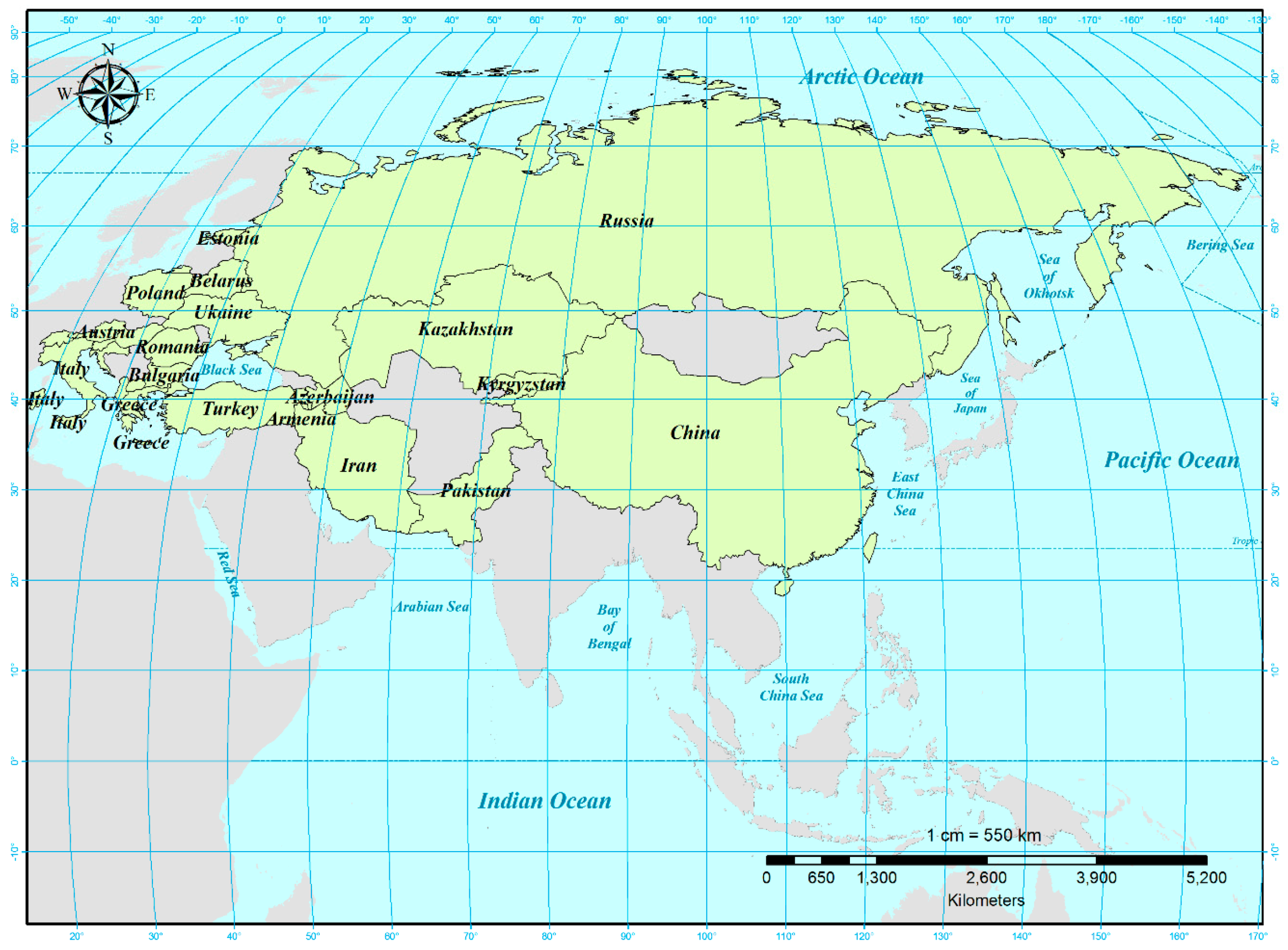
To evaluate the status of the social economy and the energy environment systems of countries under BRI and to test the spatial dependence of neighborhoods, a new integrated model that combined the coupling coordinated model with spatial econometrics was proposed in this study. In time series, the coupling coordinated model was adopted to quantify the tendency of the coupling coordinated degree of the social economy and the energy environment systems. Moran’s I method was used to calculate the spatial cluster of the research zone from 1997 to 2014 to indicate spatial dependence. The spatial panel data model was applied to test the positive or negative impact of spatial dependence based on Moran’s I. Finally, the economy connection and spatial dependence of the environment were explored to answer the question on whether BRI has no negative effect on the relationship of economy to energy and environment.

2. Methodology

The method was divided into three parts. First, the entropy model was combined with the coupling coordinated model to estimate the relationship between the social economy and the energy environment subsystems in time series. The result was then used to observe the tendencies of the social economy and the energy environment. Second, the global and local Moran’s I were adopted in the spatial scale to describe the spatial cluster of the coupling coordinated degree of the countries included in the research. Whether neighborhood exerts a spatial indirect impact is determined in this section. Finally, the spatial panel data model was applied to explain the positive or negative impact of neighborhood.

2.1. Coupling Coordinated Model

The coupling coordinated model was widely used to uncover the relationships between the different systems in nation, province, and industry scale [16,18,41]. The result of coupling coordinated model was not constrained by the spatial scale and was demonstrated by the status of the different systems [15,42]. Therefore, the coupling coordinated model was adopted in the paper to explore the relationship between the social economy and the energy environment. The status of the social economy subsystem in the research zone was represented by the variable F(x). Meanwhile, the status of the energy environment subsystem was represented by the variable G(y). F(x) was calculated using Formula 1, whereas G(y) was obtained using Formula 2, as follows:

$$F\left(x\right)={\displaystyle \sum }_{i=1}^n{w}_i{f}_i$$

(1)

$$G\left(y\right)={\displaystyle \sum }_{j=1}^m{w}_j{f}_j$$

(2)

where wi is the weight of the ith index in the social economy subsystem, αj is the weight of the jth index in the energy environment subsystem, fi is the normalized value of the ith index in the social economy subsystem, and gj is the normalized value of the jth index in the energy environment subsystem. The weight was calculated in accordance with the entropy model.

The coupling level of the social economy and energy environment subsystems was estimated using Formula 3, as follows:

$$\mathrm{U}=2\times \sqrt{\frac{\left(F\left(x\right)\times G\left(y\right)\right)}{\left(F\left(x\right)+G\left(y\right)\right)}}$$

(3)

The coordinated level of the social economy and energy environment subsystems was calculated using Formula 4, as follows:

$$V=\alpha \times F\left(x\right)+\beta \times G\left(y\right)$$

(4)

where α and β are the weights of the two subsystems, and α and β are equal to 0.5.

The coupling level was combined with the coordinated level, and coupling coordinated development was obtained using Formula 5, as follows:

$$\mathrm{D}=\sqrt{U\times V}$$

(5)

2.2. Moran’s I

Moran’s I is the most popular method for indicating the spatial cluster of a neighborhood. Moran’s I was applied to test the spatial dependence or heterogeneity of the coupling coordinated degree in the research zone. Moran’s I was calculated using Formula 6 [43], as follows:

$$I=\frac{n}{{{\displaystyle \sum }}_{i=1}^n{{\displaystyle \sum }}_{j=1}^n{\omega }_{i,j}}\times \frac{{{\displaystyle \sum }}_{i=1}^n{{\displaystyle \sum }}_{j=1}^n{\omega }_{i,j}\left(D_i-\overline{D}\right)\left(D_j-\overline{D}\right)}{{{\displaystyle \sum }}_{i=1}^n{\left(D_i-\overline{D}\right)}^2}$$

(6)

where Di is the coupling coordinated degree of ith country in BRI, i≠j, and ωi,j is an element in the i-th row and j-th column of a spatial weight matrix W that is equal to 1 if regions i and j are adjacent and to 0 if regions i and j are non-adjacent. The numbers in the spatial weight matrix W are row-standardized, i.e., the sum of the elements in each row is equal to 1. If the test results reject the null hypothesis of no spatial correlation, then the observations exhibit spatial correlation.

2.3. Spatial Panel Data Model

The spatial panel data model was a widely applied tool in both in science and social science fields [44,45]. It was used to calculate and estimate the effects of one social attribute in a zone on the same attributes in the adjacent zone [46]. In the paper, the spatial panel data model was applied to explore the relationship of the coupling coordinated degree between the countries in BRI. Given the lack of heterogeneity tests, the spatial panel data model, instead of the spatial sectional data model, is typically adopted to test the indirect effect of a neighboring country. The normal form of the spatial panel data model is shown in Formula 7.

$$\mathrm{D}=\lambda \left(I_T\otimes W_N\right)D+X\beta +u$$

(7)

where D is the dependent variable matrix; it represents the coupling coordinated degree in this study. X is the independent variable matrix, I_T is the T-order identity matrix, λ is the spatial coefficient, β is the coefficient, and u is the disturbance vector that can be calculated using Formula 8, as follows:

$$\mathrm{u}=\left(l_T\otimes I_N\right)\mu +\xi$$

(8)

where I_T is the 1 × T-order matrix, the elements of which are all 1. I_N is the N-order identity matrix, μ is the individual effect coefficient, ξ refers to the spatial error item and can be calculated using Formula 9, as follows:

$$\xi =\left(I_T\otimes W_N\right)\xi +v$$

(9)

where ρ is the spatial autoregression coefficient that represents the positive or negative impact of the independent variable on the neighborhood, and W_N is the spatial weight matrix.

In this study, the values of the global and local Moran’s I and the test of the spatial panel data model were obtained from software R with packages SPLM and SPDE [47,48].

3. Case Study

3.1. Research Zone

In 2013, the Chinese government proposed the global economic development project, namely BRI, which was rooted from the famous ancient trade path that connected China to Europe. Similar to the ancient Silk Road, BRI provides the chance of economic success and social prosperity to countries belonging to the Belt and the Road. However, BRI is not only a geographic scope but also an international cooperation and global governance form that pursues world peace and development [49]. Thus, BRI is open and inclusive; countries with peace and development aspirations can join the project [50]. Most countries in Southeast Asia, South Asia, West Asia, and Central and Eastern Europe are included in BRI. The 23 countries that belong to the Silk Road Economic Belt were selected in accordance with the principle of spatial adjacency, which considers the completeness and validity of statistical data and easy analysis, as shown in Figure 1. From the geographic zone, the countries were in five divisions, as shown in

Table 1. The countries in research zone.

Divisions	Country	Total
East Asia	China	1
Central Asia	Kazakhstan, Kyrgyzstan, Pakistan	3
West Asia	Iran, Turkey	2
East Europe	Armenia, Azerbaijan, Estonia, Belarus, Russia, Ukraine, Bulgaria, Romania	8
Central and South Europe	Macedonia, Greece, Poland, Hungary, Croatia, Slovenia, Austria, Switzerland, Italy	9

.

3.2. Data

In accordance with the social economy and the energy environment levels of the countries in the research zone, 17 indexes were set in the multicriteria assessment system for quantifying the coupling coordinated development degree. In the social economy subsystem, GDP per capita, industry added value, service added value, arable land, urbanization, research and development expenditures, and high-technology exports were adopted to reflect the macroscale, economic structure, and development trend of the social economy. Meanwhile, the energy intensity level of primary energy, fossil energy consumption, energy net import, CO₂ emissions, electricity access, CO₂ damage, particulate emission damage, and natural resource depletion were applied to evaluate the energy consumption, energy structure, environment damage, and natural resource usage in the research zone. In time series, the data of the 17 indexes from 1997 to 2014 were obtained from the world development index dataset in the World Bank Database.

4. Result and Discussion

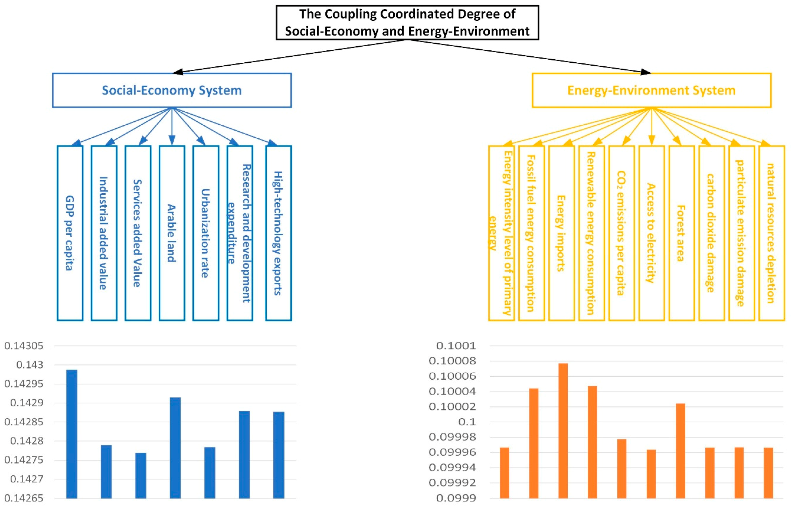
4.1. Coupling Coordinated Degree

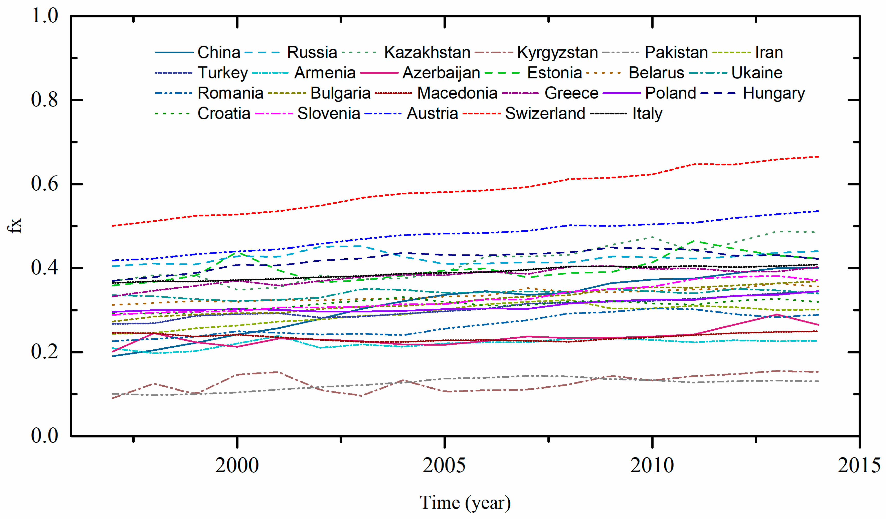
The weights of the indexes of the assessment criteria system are shown in Figure 2 in accordance with the entropy model and data. Based on weights, the coupling coordinated degrees of the countries in the research zone were calculated using the method presented in Section 2 and the data provided in Section 3. F(x) reflects the level of the social economy subsystem from 1997 to 2014, as shown in Figure 3. The result indicated that the social economy level of the countries tended to increase in time series. From the spatial point of view, Central and Southern Europe had the highest social economy level. East and West Asia had moderate social economy level. By contrast, Central Asia had the lowest social economy level. The social economy level of Eastern Europe is heterogeneous. The social economy level of Russia is the fourth highest. Meanwhile, Armenia had the third lowest F(x) value. When the spatial scale was combined with time series, the result showed that the Matthew effect was evident. Developed countries, such as Switzerland and Austria, in Central and Southern Europe, achieved the highest economic growth rate. For accelerated development, China had the highest increase in the social economy level. In 1997, the F(x) value of China was 0.19 and only slightly higher than those of Kyrgyzstan and Pakistan. In 2014, the F(x) value of China increased to 0.4 and was close to those of Russia and Italy. By contrast, developing countries exhibited slight or no development in social economy. For example, the F(x) value of Kyrgyzstan was 0.09 in 1997 and 0.13 in 2014. That is, development was extremely limited over 18 years.

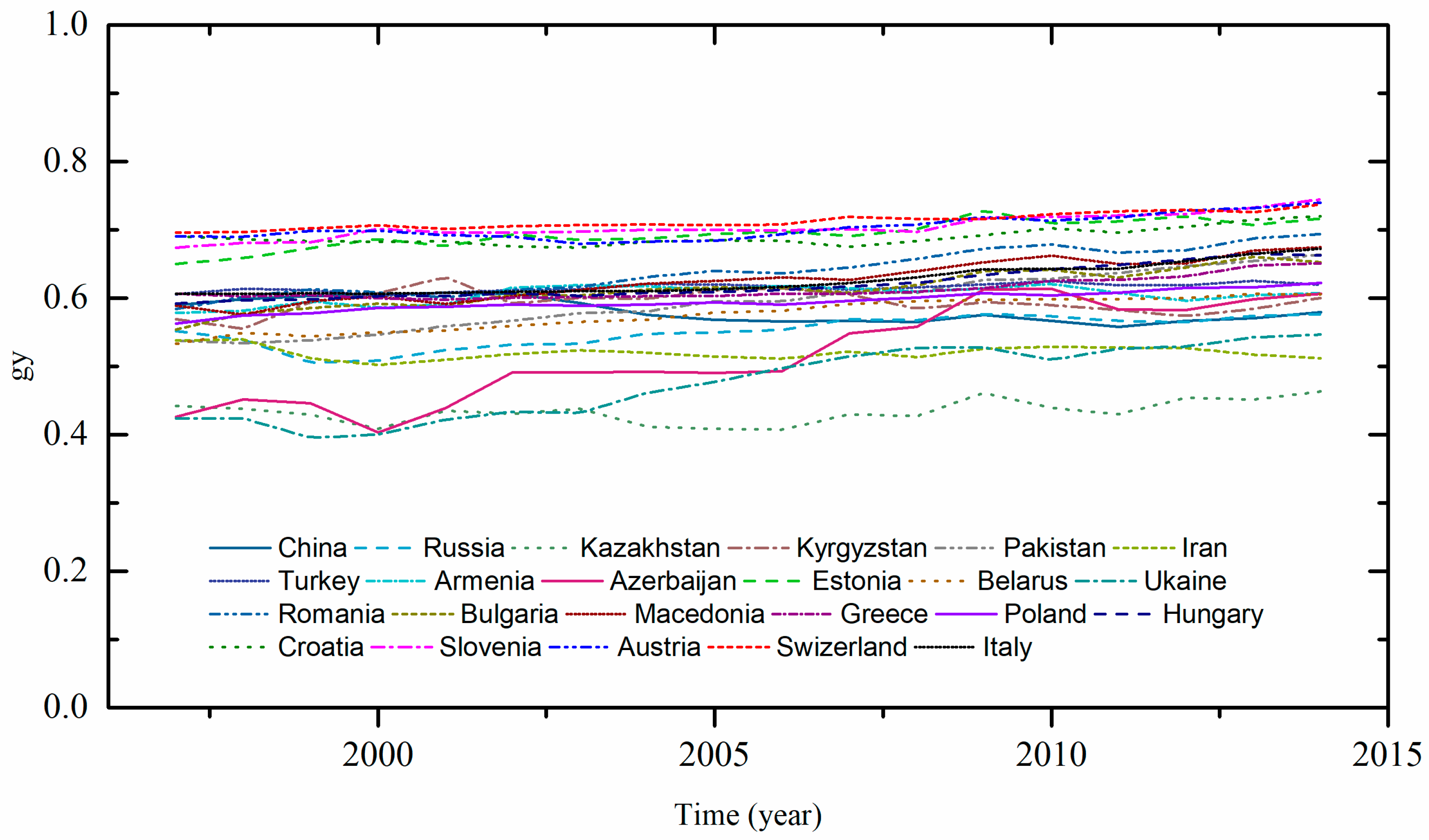
The result of G(y), which reflects the level of the energy environment subsystem in time series and spatial scale, is shown in Figure 4. In contrast with F(x), G(y) exhibited no evident heterogeneity among the countries in the research zone. The change in the value of G(y) was smaller compared with that in F(x). The regional cluster phenomenon was evident in the spatial scale. The countries in Central and Southern Europe, such as Switzerland and Austria, had higher energy environment levels. By contrast, lower levels were observed in countries, such as Ukraine and Azerbaijan, from Eastern Europe. Similarly, Iran and Kazakhstan had the lowest energy environment levels. The value of G(y) was higher than that of F(x).

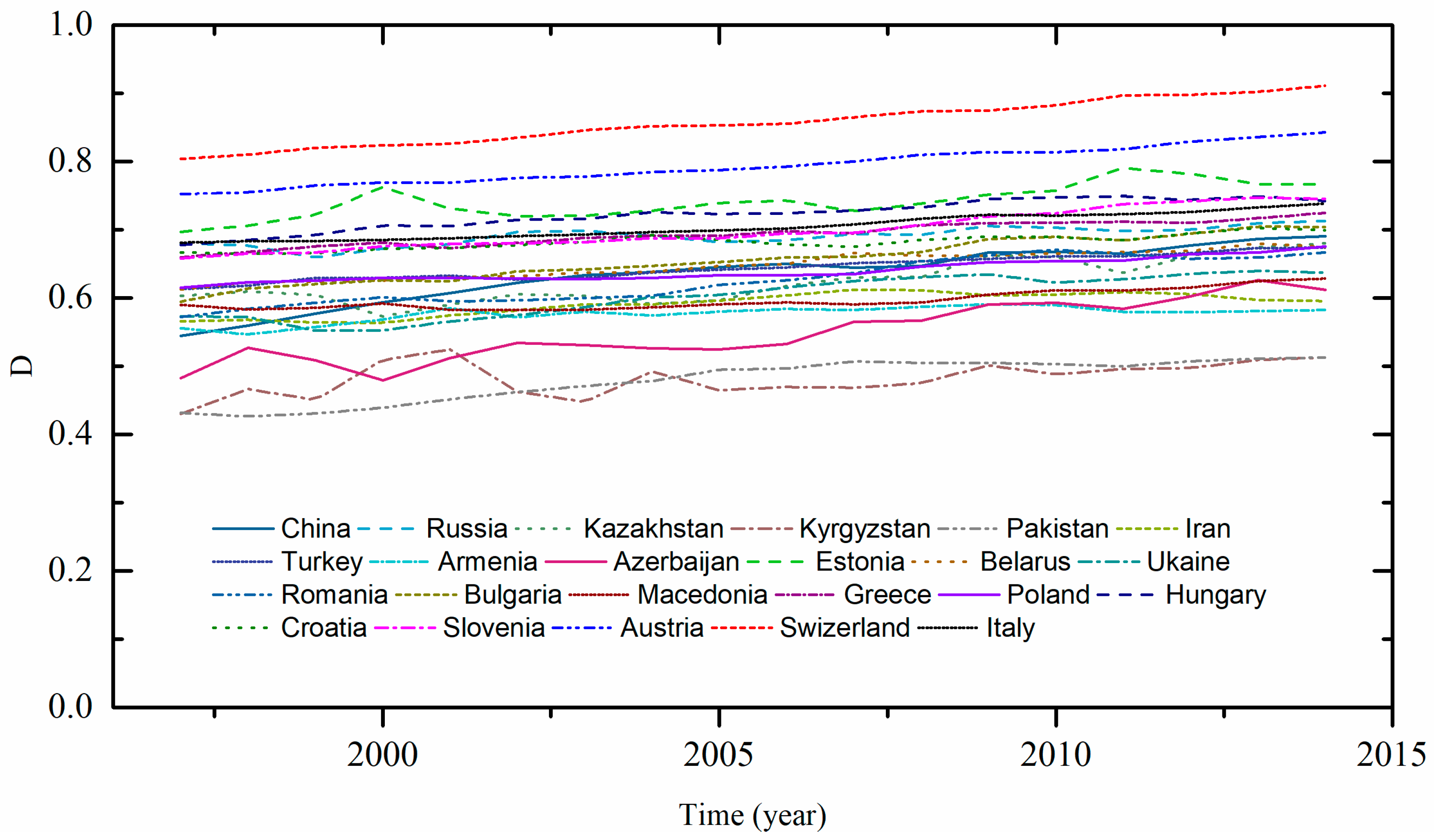
The relationship between the social economy and the energy environment was reflected by the coupling coordinated degree. As shown in Figure 5, the D value of Switzerland was the highest, followed by that of Austria. By contrast, Pakistan and Kyrgyzstan had the lowest coupling coordinated degree. In time series, the coupling coordinated degree increased from 1997 to 2014. From the change tendency, China demonstrated the highest ascending speed of coupling coordinated development. In 1997, the D value of China was 0.54; in 2014, it rose to 0.69. The second highest growth rate was achieved by Azerbaijan. The shape of the curves of the coupling coordinated degree indicated that countries with a high level of the coupling coordinated degree frequently have a steady development process. By contrast, countries with the lowest level of the coupling coordinated degree exhibited evident fluctuation in the curve. In the spatial scale, Central and Southern Europe had the highest value of the coupling coordinated degree. In this region, Switzerland and Austria had the highest levels of the social economy and the energy environment subsystems. In contrast with Central and Southern Europe, countries in Central Asia, such as Pakistan and Kyrgyzstan, had the lowest D value. When the two regions were compared, the other sections had a moderate level of the coupling coordinated degree.

4.2. Moran’s I

The global Moran’s I was calculated every year from 1997 to 2014 based on the assessment of the coupling coordinated degree. The result of the global Moran’s I is shown in

Table 2. The change of the global Moran’s I in time series.

Year	D	p	fx	p	gy	p
1997	0.46	0.001	0.26	0.026	0.22	0.048
1998	0.47	0.001	0.27	0.027	0.3	0.015
1999	0.49	0.0003	0.23	0.038	0.3	0.015
2000	0.51	0.0003	0.31	0.011	0.28	0.02
2001	0.51	0.0008	0.29	0.015	0.24	0.037
2002	0.46	0.0012	0.21	0.024	0.3	0.013
2003	0.45	0.0004	0.21	0.024	0.29	0.015
2004	0.50	0.0005	0.24	0.024	0.28	0.019
2005	0.48	0.0009	0.19	0.024	0.26	0.025
2006	0.45	0.001	0.12	0.024	0.26	0.024
2007	0.42	0.0006	0.12	0.024	0.31	0.01
2008	0.46	0.0008	0.14	0.024	0.4	0.0018
2009	0.44	0.001	0.15	0.024	0.42	0.0013
2010	0.44	0.0005	0.13	0.024	0.42	0.0013
2011	0.46	0.0007	0.19	0.024	0.43	0.001
2012	0.45	0.0005	0.18	0.023	0.5	0.0002
2013	0.46	0.0004	0.17	0.024	0.5	0.0002
2014	0.46	0.0004	0.17	0.023	0.47	0.0004

. The level of the social economy subsystem in the countries included in the research zone was more than zero based on the global Moran’s I, thereby indicating positive spatial autoregression relationships among them. In time series, the value of Moran’s I fluctuated from 0.111 to 0.155. The change in the value of Moran’s I denoted that the spatial cluster phenomenon in the social economy occurred in the countries along BRI. By contrast, the level of the energy environment subsystem of the countries in the research zone was close to zero based on the global Moran’s I. Such a result indicated that the spatial autoregression phenomenon of the energy environment was evident in the research zone. The global Moran’s I of the coupling coordinated degree was considerably more than zero. From 1997 to 2014, the value of Moran’s I in terms of the coupling coordinated degree changed within the range of 0.423–0.513. The spatial cluster phenomenon of the coupling coordinated degree was more significant in the research zone. The comparison of the Moran’s I of D, F(x), and G(y) in time series showed that the change in the coupling coordinated degrees of the countries along BRI was homologous in the entire research zone. However, the social economy and the energy environment could be heterogeneous in different regions of the research zone. Thus, the spatial autoregression phenomenon in every country in the research zone was indicated by the local Moran’s I. For the spatial dimension, the different spatial cluster types of local Moran’s I are shown in Figure 6, Figure 7, Figure 8 and Figure 9.

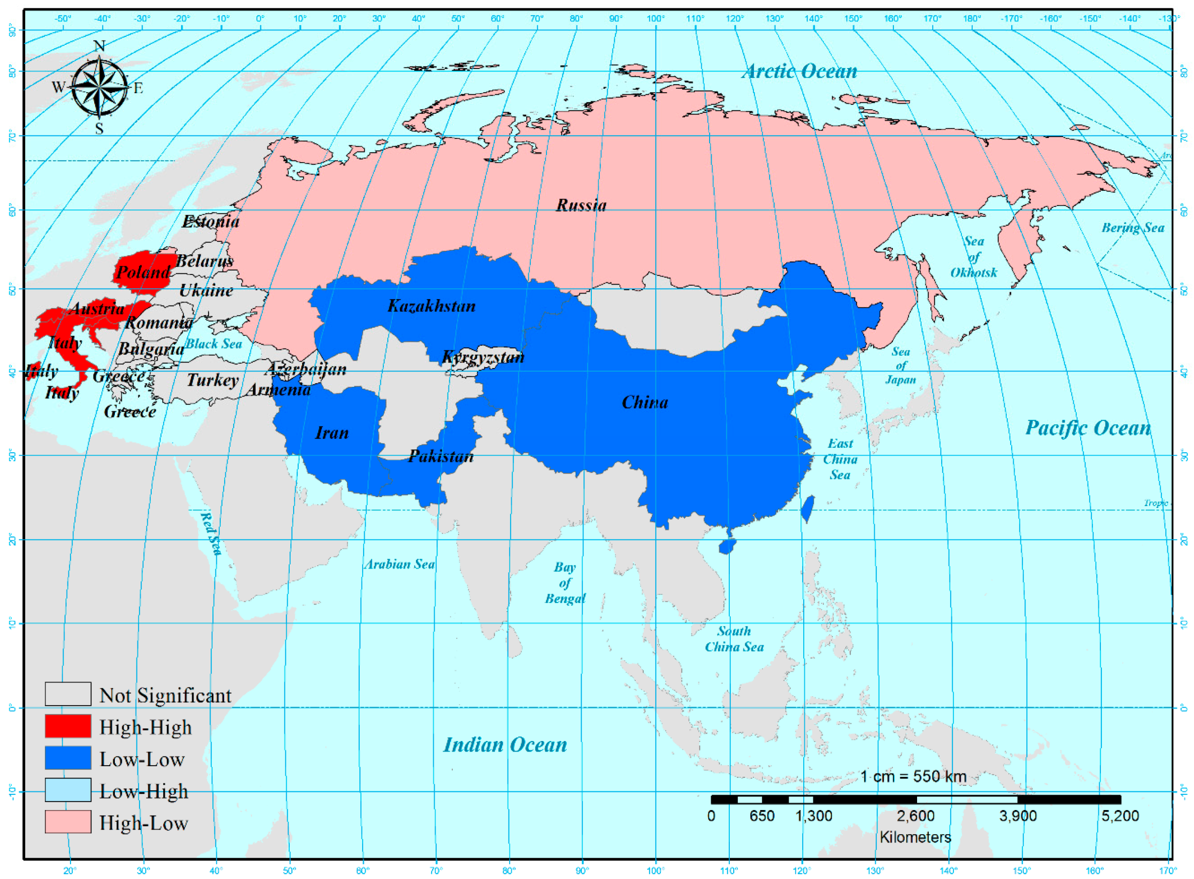
As presented in Figure 6, the local Moran’s I of the coupling coordinated degree in 1997 was in the form of a local indicators of spatial association (LISA) map. The result demonstrated that the spatial cluster phenomenon was evident in different sections. In East and Central Asia, China, Pakistan, Kazakhstan, and Iran exhibited low–low spatial autoregression relationship with neighboring countries. By contrast, the countries in Central and Southern Europe, such as Switzerland, Austria, Italy, and Poland, demonstrated high–high spatial autoregression relationship with their neighbors. The LISA map of Moran’s I in 1997 interpreted the global Moran’s I because the positive value of the global Moran’s I reflected the low–low and high–high types of spatial cluster. Thus, the global Moran’s I was positive when the low–low and high–high spatial cluster types were dominant. In 1997, the high–low spatial cluster phenomenon occurred in Russia. Meanwhile, the other countries in the research zone presented no evident spatial autoregression relationship.

The LISA map of the coupling coordinated degree in 2002 is shown in Figure 7. Compared with Figure 7, the spatial cluster type of Poland changed to a low–high relationship. The other countries in the research zone maintained the same spatial cluster types in 1997. As shown in Figure 8, the low–low spatial autoregression relationship was evident in Kyrgyzstan in 2008. The level of low–low spatial cluster was enhanced in Central Asia. 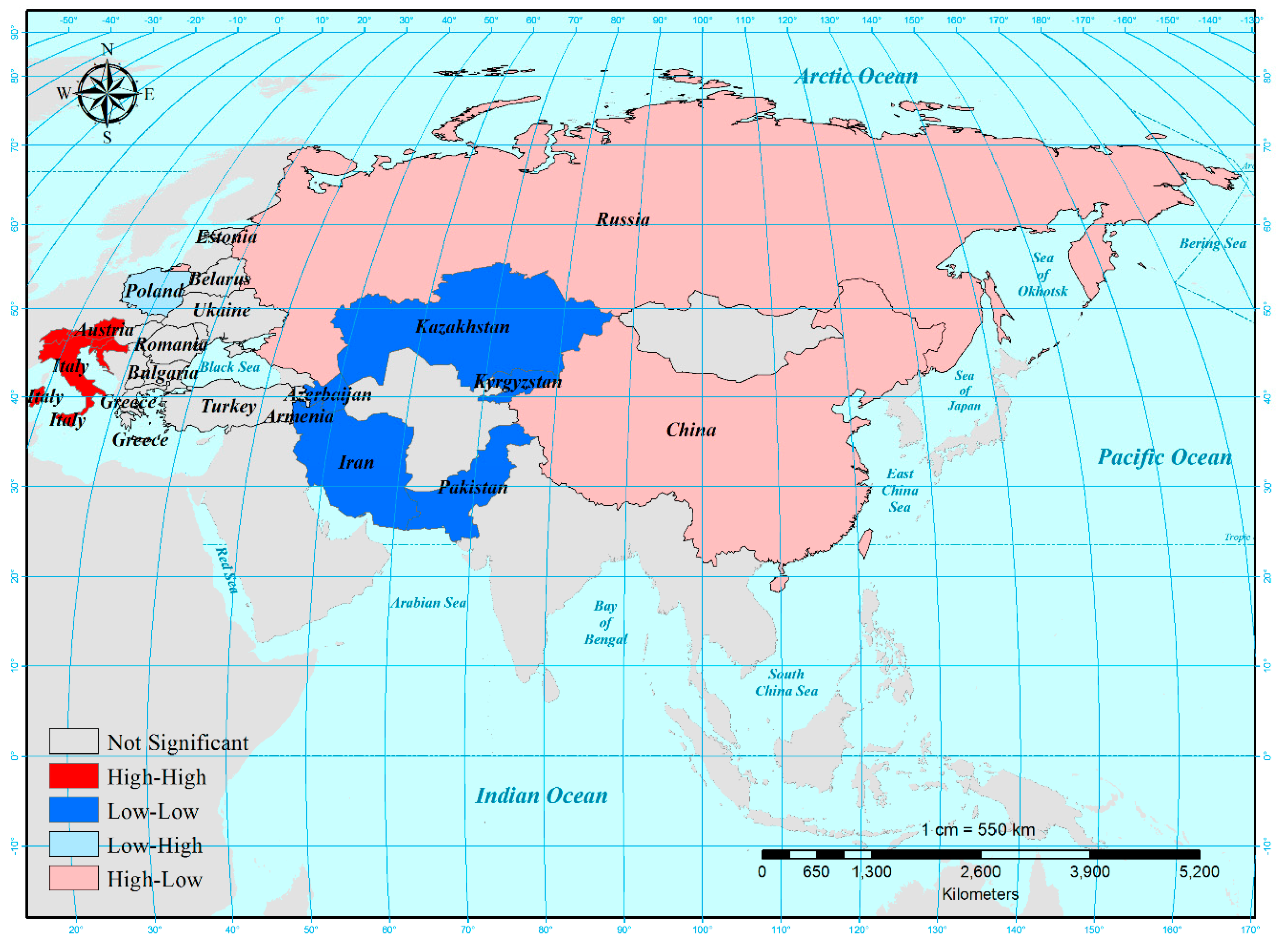Meanwhile, Figure 9 shows that the spatial cluster type in 2014 was transformed from low–low to high–low. The other countries maintained the same spatial autoregression relationships in 2008. Thus, the time series indicated that the spatial cluster phenomenon was evident in East and Central Asia and Central and Southern Europe. Similarly, Russia had a high–low spatial autoregression relationship from 1997 to 2014. The other countries had no evident relationship.

4.3. Spatial Panel Data Model

The results of Moran’s I indicated that spatial autoregression relationships existed in the research zone. However, the spatial spillover effect cannot be identified by Moran’s I. The spatial panel data model was applied to test the spatial relationship among countries in the research zone to determine the spatial spillover effect. A spatial panel dataset was constructed using the D, F(x), and G(y) of 23 countries from 1997 to 2014. D is the dependent variable, whereas F(x) and G(y) are the independent variables based on the calculation method of the coupling coordinated degree. The spatial autoregression and random effect of the panel data were tested based on the test principle proposed by Baltagi & Song [51]. The results are listed in

Table 3. The result of BSK test.

Null Hypothesis	Alternative Hypothesis	Statistic	p
spatial autoregression and random effect were nonexistent.	spatial autoregression or random effect were existent.	LMH = 2503.9	2.2 × 10−16
random effect was nonexistent.	random effect was existent.	LM1 = 19.86	2.2 × 10−16
spatial autoregression was nonexistent.	spatial autoregression was existent.	LM2 = 4.27	1.9 × 10−5

.

Table 3 shows the results of the BSK test, which indicate that the spatial autoregression and random effect occurred in the panel data. Therefore, the spatial lag model should be selected in this study. However, the random or fixed effect should be tested in accordance with the result of the Hausman test [52]. The result of this test is listed in

Table 4. The result of Hausman test.

Null Hypothesis	Alternative Hypothesis	Statistic	p
random effect was adopted	fixed effect was adopted	0.53	0.76

.

As shown in this table, the statistics and p value indicated that the null hypothesis could not be rejected. The spatial lag model with random effect was selected to interpret the spatial spillover effect. The coefficient and constant of the spatial lag model are listed in

Table 5. The estimate of spatial lag model.

Dependent Variable: log(D)	Coefficient	Std. Error	t-Value	p
μ	6.007	1.843	3.2605	0.0011
λ	0.014	0.004	3.4579	0.0005
intercept	0.157	0.0016	97.031	2.2 × 10−16
log (FX)	0.325	0.001	318.894	2.2 × 10−16
log (GY)	0.412	0.002	208.458	2.2 × 10−16

.

The estimated value and t-value in Table 4 showed that the coefficient of spatial autoregression (λ) was 0.014 and the p value of λ was 0.0005. Moreover, the λ value was positive. Thus, the coupling coordinated degree of one country demonstrated evident spatial spillover effect. The positive value indicated that the coupling coordinated degree of one country positively affected those of its neighboring countries.

4.4. Discussion

The development of the social economy was compared with the level of the energy environment in the research zone from 1997 to 2014. The result indicated that G(y) was considerably higher than F(x) in developing countries because a lower level of the social economy required less support of the energy environment. By contrast, developed countries had similar levels of the two subsystems. In Central and Southern Europe, developed countries, such as Switzerland, Austria, and Italy, completed the industrialization process, and the industrial structure of these countries was optimal. Accordingly, gaining economic success requires less energy consumption and environmental degradation in these countries. In similar developed countries, such as Croatia and Estonia, in Eastern Europe, the smaller population scale and the thriving high-value-added industry sector, such as tourism and telecommunications, accelerated economic success. Meanwhile, the development of these pillar industries was not based on the immense consumption of energy and environment. Therefore, these countries also had high levels of the two subsystems. The relationship between the two subsystems was more complex in moderately developing countries, such as Russia and China. The two subsystems in China exhibited opposite tendencies from 1997 to 2014. Benefiting from the unprecedented economic development, F(x) increased rapidly. Given the incomplete industrialization process, a high level of the social economy was required to be supported by a high level of energy consumption and environment degradation, which led to the descent in the trend of the energy environment subsystem. In Russia, energy export was the major source of income for the country. Energy price volatility directly affected the development of the social economy subsystem. From the time dimension, the phenomenon of the coupling coordinated development homogeneity was evident. The D value reflected the level of the coupling coordinated degree that increased in different degrees. Developed countries in Central and Southern Europe presented steady development of the coupling coordinated degree. Meanwhile, fluctuating development occurred in developed countries in Eastern Europe. Developing countries in Central Asia were dramatically unstable and development was slow. China and Russia, which represent moderately developing countries, exhibited fluctuating and accelerating development. Although the countries along BRI presented different forms of coupling coordinated development, the same developing tendency was observed in the entire region. Apart from the global development trend, the reason for the homogeneity in the region may not only be economic connection but also the energy and environment relationships among countries.

In the temporal dimension, the global Moran’s I showed the positive spatial cluster phenomenon in accordance with the tendency of the coupling coordinated degree. Homogeneity existed in the region. The relationship among the coupling coordinated development of countries in the research zone was proven quantitively based on the result of the global Moran’s I. However, the heterogeneity in the development of different countries could not be explained by the value of the global Moran’s I. Therefore, the local Moran’s I in the snapshots of 1997, 2002, 2008, and 2014 was adopted to indicate heterogeneity in the region. In time series, the difference in spatial distribution of the coupling coordinated degrees was evident in all periods, during which the countries in Central and Southern Europe exhibited high–high spatial cluster relationship among adjacent countries. In the Central and Southern Europe, the countries all finished the industrial process and urbanization. Switzerland, Austria, and Italy were all the developed countries with the optimal industrial structure and high productivity. Thus, the more economic success consumed, the less energy and the less pollution. Different from the three countries above, Croatia, Hungary and Slovenia had a small population and high-added-value industry such as tourism. Therefore, economic success was easier to prompt in these countries. The reverse condition occurred in East and Central Asia, where low–low spatial clusters dominated the relationships among countries. Kazakhstan, Kyrgyzstan, and Pakistan are developing countries with a low level of resource and an unreasonable industrial structure. The resources are a bottleneck of the economic development and high added value was difficult to achieve under the unreasonable industrial structure. In East Asia, the condition of China is different from the three countries in Central Asia. China had the highest scale of population, which gives it high energy consumption and pollution emissions meeting the need for huge population scale. The result indicated the heterogeneity in different sections of the region. From the change in the local Moran’s I in time series, Central and Southern Europe and Central Asia exhibited no change in spatial cluster types. By contrast, developed countries in Eastern Europe, such as Poland, presented dramatic changes in spatial relationships. However, the scope of the high–high spatial cluster in Central and Southern Europe had no tendency to expand in time series. Conversely, countries with low–low spatial cluster in East, Central, and West Asia increased by 2014. Thus, the spatial connections of the coupling coordinated development of the social economy and energy environment in this section were strengthened, although spatial clustering was low–low. In 2014, low–low spatial clustering type in China was converted to high–low. To test the connections of the coupling coordinated development in the entire research zone and the transformation of the spatial cluster types in the future, the spatial spillover effect was verified using the spatial panel data model. The result of the spatial panel data model showed that a positive spatial spillover effect existed in the research zone. Therefore, the advance of the coupling coordinated degree in one country was the driving factor of the increase in the coupling coordinated degrees of its neighboring countries. Combined with the result of the local Moran’s I, the scope of the spatial cluster would expand in the future, and the status of the spatial cluster in Asia from 1997 to 2014 verified the result of the spatial panel data model analysis. However, Central and Southern Europe, which had high–high spatial cluster type, did not expand. That is, the positive spatial spillover effect was significant in Asia. Meanwhile, the spatial cluster type of China was converted to high–low in 2014. Thus, the level of the coupling coordinated development of China was higher than those of adjacent countries. The high level of the coupling coordinated degree of China was the promoting factor that enhanced the level of the coupling coordinated degrees of its neighboring countries because of the positive spatial spillover effect in Asia.

5. Conclusions

To interpret the problem, the coupling coordinated degree model was adopted to estimate the direct relationship between the social economy and the energy environment. Then, the spatial econometric model was applied to test the spatial relationships among the countries in BRI. The result showed the indirect relationship among the coupling coordinated degrees of adjacent countries. The 23 typical countries along BRI constituted the research zone. The level of the coupling coordinated development from 1997 to 2014 was evaluated. In the spatial dimension, the coupling coordinated degrees of countries demonstrated the phenomenon of spatial heterogeneity based on the assessment result. By contrast, the coupling coordinated degrees of countries exhibited temporal homogeneity. Moran’s I was used to verify the spatial autoregression relationship, and the result of Moran’s I explained temporal and spatial heterogeneities. The spatial panel data model was adopted to test the spatial spillover effect. The result of the spatial panel data model determined the tendency of the coupling coordinated degree in the research zone.

The result showed that Central and Southern Europe obtained the highest level of coupling coordinated development. However, the spatial connection in this zone should be strengthened. By contrast, countries in Central Asia had the closest spatial relationship among adjacent countries. Meanwhile, a low level of development occurred in this zone. Therefore, the countries in Central, East, and West Asia should complete their industrialization process to enhance the social development level and reduce energy consumption and environment degradation. The countries in Central and Southern Europe strengthened regional connections to promote coordinated development in the region. Finally, the result showed that China positively affected the coupling coordinated development of its neighboring countries.

In the paper, the spatial lag model with random effect was selected as the tool to analyze the spatial connections. However, regional heterogeneity in the data was not considered to avoid bias in the non-spatial effects. Thus, the spatial Durbin panel model was adopted to estimate the local spatial spillover effects in our future work.