Urban Rail Timetable Optimization to Improve Operational Efficiency with Flexible Routing Plans: A Nonlinear Integer Programming Model

Abstract

At present, most urban rail transit systems adopt an operation mode with a single long routing. The departure frequency is determined by the maximum section passenger flow. However, when the passenger flow varies greatly within different sections, this mode will lead to a low load factor in some sections, resulting in a waste of capacity. In view of this situation, this paper develops a nonlinear integer programming model to determine an optimal timetable with a balanced scheduling mode, where the wasted capacity at a constant departure frequency can be reduced with a slight increase in passenger waiting time. Then, we simplify the original model into a single-objective integer optimization model through normalization. A genetic algorithm is designed to find the optimal solution. Finally, a numerical example is presented based on real-world passenger and operation data from Beijing Metro Line 4. The results show that the double-routing optimization model can reduce wasted capacity by 9.5%, with a 4.5% increase in passenger waiting time, which illustrates the effectiveness of this optimization model.

1. Introduction

With the growth of the urban population, traffic demand has gradually increased in China. Urban rail transit has become an important part of urban public transportation with the advantages of safety, high efficiency, convenience, reliability, low energy consumption and light environmental pollution [1]. Making full use of urban rail transit is an important way to relieve the pressure of modern urban traffic and to promote its sustainable development. The urban rail timetable is the core technical content for train operation organization. It is the guidance document for coordination among companies and its quality will affect passenger satisfaction and operation cost [2]. The idea of a reasonable timetable, which can command train operation, ensure traffic safety and improve transportation efficiency, is attracting more and more attention. Therefore, it is significantly important to optimize metro timetables in order to improve operational efficiency.

At present, urban rail transit is mostly operated on the single long routing mode. With the city gradually extending outwards, a lot of radial lines connecting the urban central area to the suburbs and radial lines connecting suburbs at both ends of the urban area, have been formed. The passenger flow on these lines is unevenly distributed in each section. If trains are still operated on a single long routing mode and the departure frequency is determined by the maximum section passenger flow, this will cause a great capacity waste in some sections. For this phenomenon, some cities are actively exploring the operation method of mixed operation on double routings—Shanghai Metro Line 1, Guangzhou Metro Line 2 and Tokyo Metro Line 3, for example. At present, train routing plans are mostly determined by the operator’s experience, based on the spatial distribution characteristics of passenger flow along the line, combined with the actual line condition, lacking systematic and quantitative research. Therefore, it is necessary to study train operation plans which systematically use mixed operation on long and short routings.

2. Literature Review

The method of mixed operation on double routings was first used in public bus services. As early as 1987, coordination modes to find the schedule offset between different routings were used to balance loads and minimize overall cost, where the primary objective was to minimize fleet size and the secondary objective was to minimize waiting time for a given fleet size. It was shown that even when overall capacity exceeds volume on every link, there may still be one or more patterns of trip schedule that are not systematically overcrowded [3]. Cristián et al. [4] found that the mixed routings strategy can be justified in many cases with uneven load patterns. Since then, an extensive variety of models for mixed operation on double routings have been proposed by researchers. The researches mainly focused on operation cost and the main purpose was either to minimize the total cost or maximize the total benefit. Ji et al. [5] studied an optimization model on bus routes to reduce the total cost. The model optimized the schedule coordination of a long routing service mode and a short-turning service mode and balanced the bus load along the route and between the two service patterns.

The relationship between operation cost and energy consumption is inseparable. With the widespread concern surrounding energy consumption, the issues of how to reduce energy consumption and capacity waste have become important for researchers. Yang et al. [6] developed a cooperative scheduling approach to optimize the timetable so as to improve the utilization of recovery energy. Yu et al. [7] established a two-stage model of a high-speed rail train operation plan. In the first stage, the proposed model aimed for the minimum total cost of train operation, which generated fewer train candidate sets, thereby improving the efficiency of the solution. In the second stage, the model gave an accurate flow distribution model to obtain the optimal economic efficiency and completed the design of the high-speed express train operation plan.

In addition to energy consumption, service level is also important for operators. Szeto and Wu [8] proposed a model to reduce the number of transfers and the total travel time of passengers, thereby improving upon existing bus services. An integrated solution method was achieved to simultaneously determine the departure frequency and operating route. Cadarso and Marín [9] developed an integrated planning model to readjust departure frequencies by recalculating the railway timetable and rolling stock. The purpose of the model was to cater for increasing passenger demand and to better adjust these flows to passenger demand, thereby alleviating traffic congestion around urban and suburban areas. Canca et al. [10] described a short-turning strategy to optimize train operation; the optimization objective was to diminish the passenger waiting time and preserve a certain level of service quality. The model determined the service offset and turn-back stations. Huang et al. [11] constructed a load balancing approach to optimize metro train operation. The model was based on an improved route which generalized the time utility function, considering the penalties of both in-vehicle congestion and transfers, thereby improving the service quality and reducing safety risks in metro systems, at the same time.

Many researchers considered reducing energy waste and improving service quality, at the same time. Sun et al. [12] put forward a multi-objective optimization model by studying specific methods on train routing to optimize high-speed railway network operation. The model considered energy consumption and trains’ average travel time and also took user satisfaction into account. Yang et al. [13] formulated a two-objective integer programming model to decrease the passenger waiting time and increase the utilization of regenerative energy, simultaneously. The model optimized the train timetable by controlling the train’s headway time and dwell time. D’Acierno and Botte [14] developed an analytical approach to deciding driving strategies. The framework could be used for properly supporting the implementation of eco-driving strategies, from a passenger-oriented perspective. The numerical examples showed that the proposed approach is useful in determining the optimal compromise between travel time increase and energy decrease. Wang et al. [15] investigated a multi-objective vehicle-routing optimization problem, where the objectives aimed to minimize total energy consumption and customer dissatisfaction, simultaneously. The study found a better balance between energy consumption diminishment and customer satisfaction and, finally, developed a mixed integer programming model to address the problem. Sun et al. [16] developed a multi-objective timetable optimization model to minimize total passenger waiting time and energy consumption. The model was verified by real-world smart-card automated fare collection data and it was shown that the developed model could improve passenger service and reduce pure energy consumption more efficiently in comparison with the timetable used currently.

Many researchers considered reducing operation cost and improving service quality, at the same time. Site and Filippi [17] chose the net benefit composed of user waiting times minus operator costs as the objective function and developed an optimization framework to obtain the maximum net benefit. The framework gave thought to variable vehicle size and service patterns over different operation periods so as to obtain an intermediate-level planning of bus operations. Chang et al. [18] applied mixed operation on double routings to rail transit and a multi-objective programming model was developed to minimize the total cost, combining the passengers’ total travel time loss and the operator’s total operating cost. Based on the analysis of an urban rail transit train plan and users’ travel expenses, Deng et al. [19] developed a multi-objective optimization model to reduce passengers’ general travel expenses and increase the operator’s benefits, simultaneously. Codina et al. [20] presented a model balancing construction costs, operational costs and passengers’ benefits. The mode optimized users’ travel times and designed a public transit network system using the traditional approach of transport demand coverage in bimodal scenarios of operation. An and Zhang [21] constructed a mixed integer programming model to minimize the cost while improving transit service. The model composited bus-holding and stop-skipping strategies to obtain a real-time optimal strategy and was solved by a Lagrangian relaxation algorithm. The study found a better balance between the quality of the transit service and the operation cost.

In some special cases, a mixed operation of double routing can also be used. Considering rotating maintenance, rolling stock circulation plans and a long-term maintenance policy, Canca et al. [22] proposed a mixed integer programming model to minimize wasted capacity caused by train empty movements and to balance the workload of the maintenance operation. Cadarso et al. [23] presented an integrated model for the recovery of the timetable and the rolling stock schedules, so that the recovery schedules could be easily implemented in practice and the operations could quickly return to the originally planned schedules after the recovery period. Cadarso et al. [24] proposed an approach synthetically considering the influence of passengers’ behavior, the timetable and rolling stock. It combined two models: one which was an integrated optimization model for the timetable and rolling stock and another which was a model for the passengers’ behavior. The proposed approach could quickly find the best solution in two steps and with a very good balance between various managerial goals.

In summary, a large number of double routing operation models have been developed and the main optimization is to determine the return site and the departure frequency. On the basis of the aforementioned models, the purpose of this study is to develop a double-routing optimization model to minimize the objective function combining the passenger waiting time and the wasted capacity on the balanced scheduling mode, so as to obtain better capacity matching.

Compared with previous studies, this study presents the following differences:

• Compared with Deng et al. [19], in which the turn-back station cannot be changed, the model established in this manuscript is used to first make decisions on the turn-back station.
• Compared with Deng et al. [19] and Chang et al. [18], this manuscript determines the routing which the train should be operated on at x_i time on the basis of considering the departure frequency and train capacity. Fleet size is not considered in this manuscript, because it changes infrequently in practice.
• Compared with Deng et al. [19] and Chang et al. [18], the single-objective model is obtained by weighted summation with two different dimensions of passenger waiting time and wasted capacity in the original model and the nonlinear integer programming model is solved based on genetic algorithms.
• Compared with Deng et al. [19] and Chang et al. [18], the relationship between the total passenger flow and the train’s optimum headway is obtained in this study, which makes it unnecessary to calculate the section passenger flow and find out the maximum section passenger flow specifically. In additional, this manuscript simplifies the algorithm for calculating departure frequency and analyzes the conditions for the double-routing operation.

Table 1. Detailed features of closely related studies.

	Turn-Back Station	Departure Frequency	Specific Departure Time	Fleet Size	Train Capacity	Implementation Method
Chang et al. (2000)	Considered	Considered	Not considered	Considered	Not considered	Fuzzy programming
Deng et al. (2013)	Not changed	Considered	Not considered	Considered	Not considered	Three-phase solving strategy
This paper	Considered	Considered	Considered	Not considered	Considered	Genetic algorithm

shows the detailed feature comparison between closely related studies.

By optimizing the train operation plan to meet the demands of different sections’ passenger flow, the cost of transportation enterprises is reduced, under the premise that the service quality is little affected, and the efficiency of the trains used is improved. At the same time, this operation mode can alleviate wasted capacity and make the operation organization economically reasonable.

The rest of this paper is organized as follows. In Section 3, we provide the problem statement. In Section 4, we formulate an integer optimization model with the objectives of passenger waiting time and wasted capacity. In Section 5, we design a genetic algorithm (GA) to solve the formulated optimization model. Based on real-world passenger and operation data from Beijing Metro Line 4, in Section 6 we conduct a numerical example. Section 7 concludes the work.

3. Problem Statement

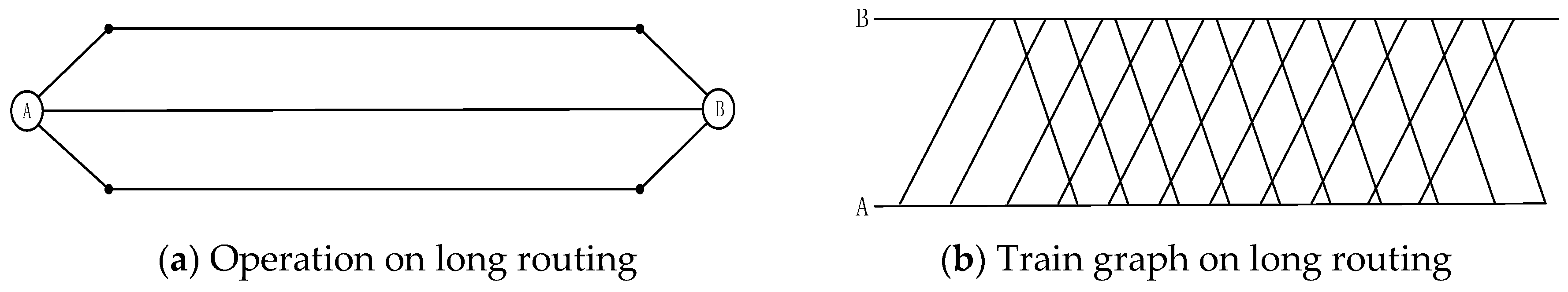
Transit timetable construction at the route level is generally based on the maximum observed passenger flow. In current practice, this maximum passenger flow is observed in a specified time period. It is divided by a load standard (desired occupancy, e.g., number of seats) to obtain the number of departures required [25]. At present, urban rail transit is mostly operated on a single long routing mode, as shown in Figure 1a and the train graph in Figure 1b. With the city gradually extending outwards, there are metro lines connecting suburbs at both ends of the urban area. The passenger flow in the urban area is very large but in the suburbs the flow is relatively small at both ends of the line, so it is suitable to use the double-routing operation mode, as shown in Figure 1c and the train graph in Figure 1d. In addition, there are metro lines connecting the urban central area to the suburbs and similarly, the passenger flow in the urban area is much larger than the passenger flow in the suburbs, so it is suitable to use a simpler double-routing operation mode, as shown in Figure 1e and the train graph in Figure 1f.

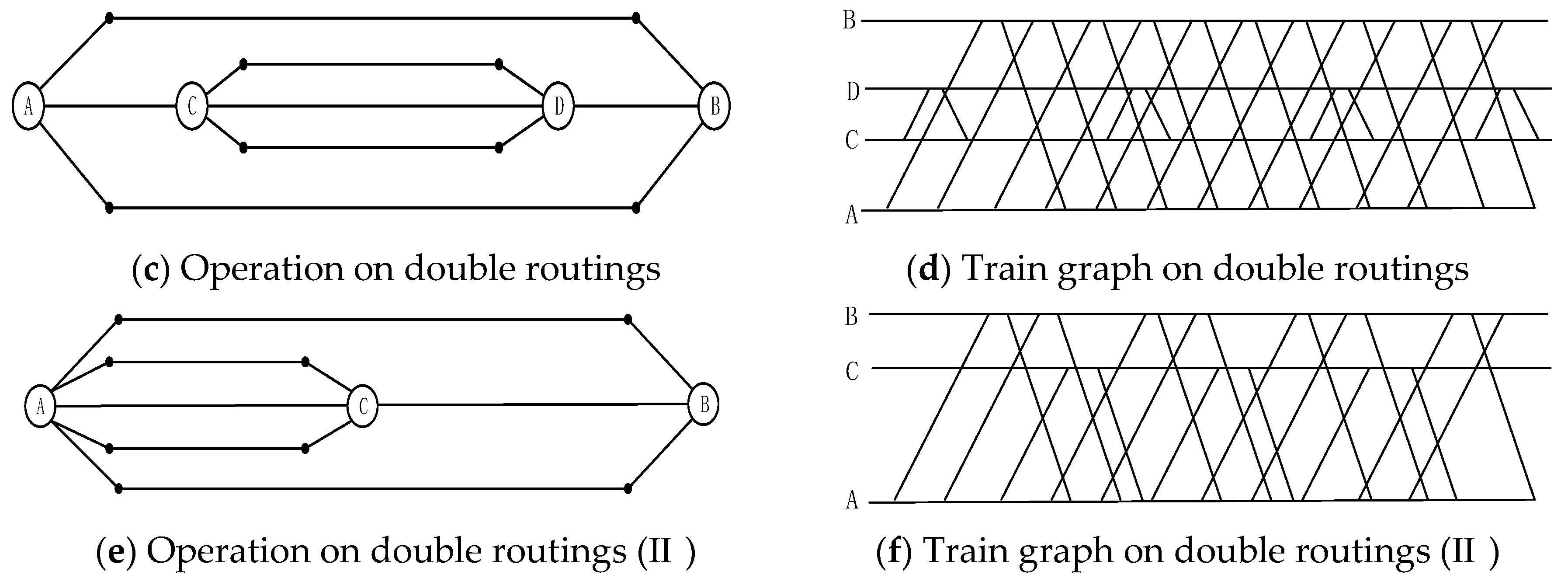
A brief description of the physical urban rail line and rolling stock is shown in Figure 2. The solid arrow stands for the long routing and the dotted arrow represents the short routing. The solid lines are the simple expression of the physical urban rail tracks. The reversing tracks have been built at station a, consequently, the train operated on the short routing can change the travel direction.

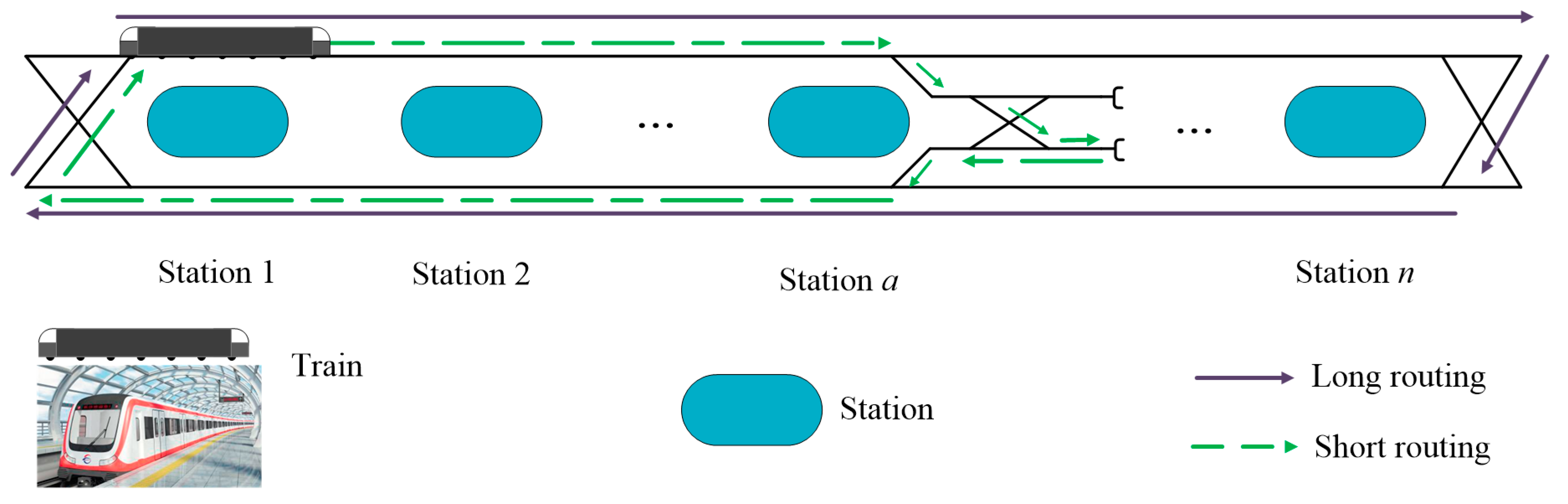
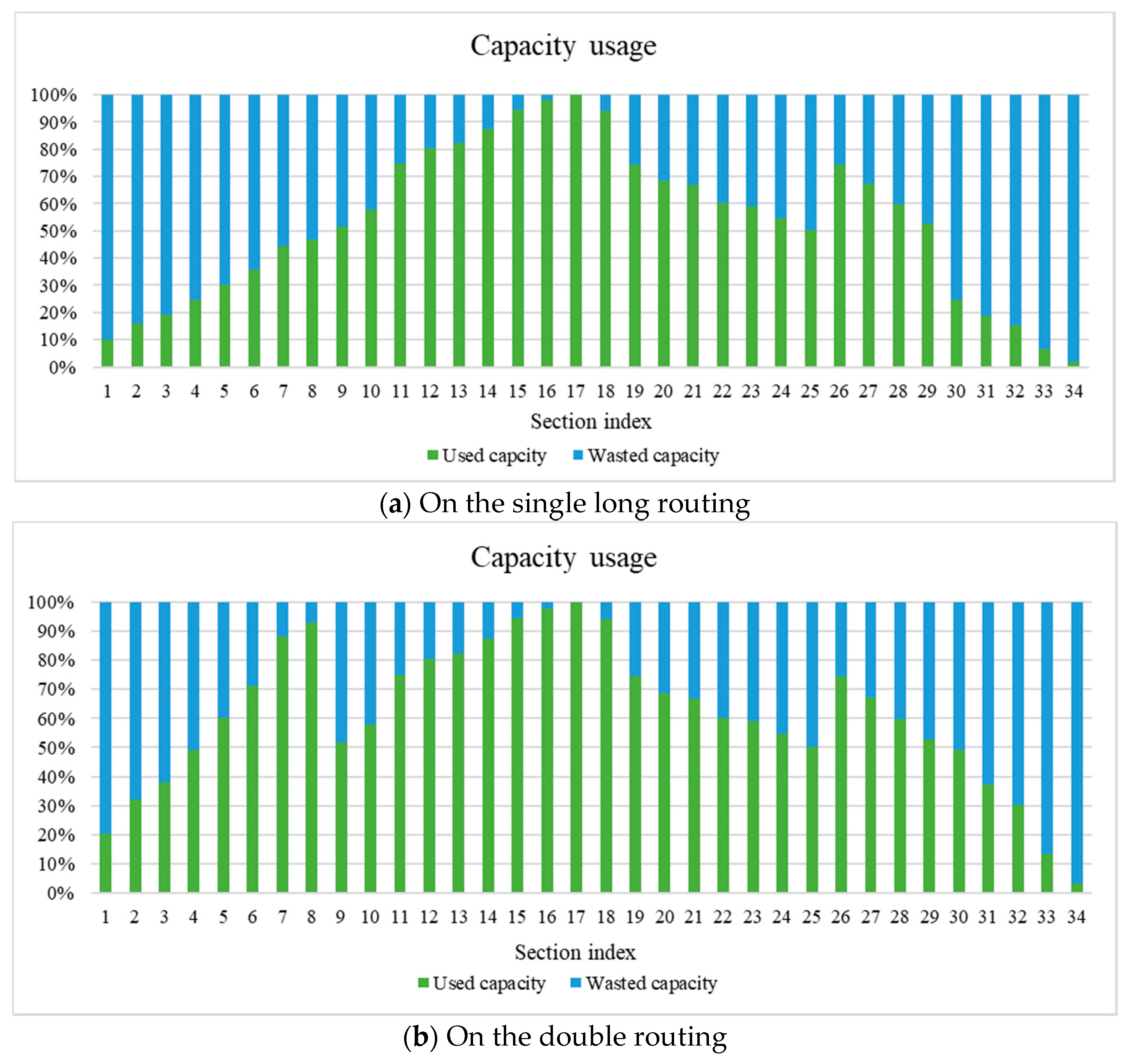
The train routing plan is an important part of the train operation plan in urban rail transit. Its formulation should be based on the full analysis of passenger flow, considering the operation organization conditions. It will directly affect the formulation of the train timetable and the rolling stock operation plan. The motivation for the double-routing operation is to promote a better match between capacity and demand. Passenger demand may vary at different times or sites. Figure 3 illustrates the spatial distribution of passenger flow and the capacity usage on each section. The spatial distribution of passenger flow reflects the difference in passenger flow in different directions and locations of the line. The usage of capacity in a single long routing is shown in Figure 3a and we can find that there is a lot of waste of capacity in many sections. In support of the idea that operators should use the double-routing operation and reduce the number of trains in sections with less passenger flow, the capacity usage on the double routing is shown in Figure 3b, in which the usage of capacity is improved on some sections.

Since many passenger demands can be met by a trip following either a full-length or short-turn pattern, schedule coordination between the patterns is essential [3]. The critical issue in short-turn service is to determine the turn-back point and the route schedule to balance passenger loads among the trips and to minimize the total fleet size and passenger waiting times. The train plan of urban rail transit under the multi-routing mode can be divided into three parts: train formation, train operation periods and the corresponding train counts of each routing in each period [19]. The design of strategies that guarantee reasonable user waiting times with small increases in operation costs is now an important research topic [10,26].

Through the above analysis, we construct a double-routing optimization model to determine the turn-back station of the short routing according to the uneven distribution of passenger flow. Then, we decide to operate on either the long or short routing at a particular time, based on the actual passenger flow. The trains on the long routing will turn back at the terminal, while the trains on the short routing will turn back at the middle station obtained by the model decision.

4. Model Formulation

This section develops a double-routing optimization model to reduce both passenger waiting time and wasted capacity, on a balanced scheduling mode. The following discussions focus on detailing each part of the formulation, that is, notions, model assumptions, objective function, system constraints and the optimization model.

4.1. Notations

To facilitate the presentation of the model in this paper, the parameters are listed below.

(1) Indices
h	station index, h = 1, 2, …, n
j	section index, j = 1, 2, …, n−1
(2) Parameters
i	the set of metro routes, I = {1, 2}, 1 on behalf of the long routing, 2 on behalf of the short routing
f	the departure frequency for operating the long routing
qo,d	the volume of passenger flow from station O to station D
Q	passenger flow matrix consisting of qo,d
tz,tz’	the minimum return time of the train at the terminal and intermediate station
I0	minimum tractive time
fmin	minimum departure frequency
Cz	rated passenger capacity
α	maximum section load factor
(3) Decision variables
X	Train operation plan, X = {xi | i = 1, 2, …, f}, xi = {1, 2}, 1 on behalf of the long routing, 2 on behalf of the short routing
a	index of return station in short routing, a ∈ {2, 3, …, n−1}
(4) Intermediate variables
Q1	total volume of passenger flow which the origin or destination is outside the short routing
Q2	total volume of passenger flow which the origin and destination are within the short routing
t1d,t2d	average passenger waiting time corresponding to Q1,Q2 respectively
Qm	actual passenger volume of metro
f1	the departure frequency of long routing
f2	the departure frequency of short routing
N1	actual capacity of long routing
N2	actual capacity of short routing

4.2. Model Assumptions

According to the actual operation characteristics of metro systems, the following assumptions are made to simplify the model formulation.

(A1). Each station in the line has the conditions for building a reversing track.

(A2). The rolling stocks are used independently for long routing and short routing.

(A3). Trains running on long routing and short routing are both operated in the mode of stopping at every station.

(A4). Trains running on long routing and short routing both have the same type and formation.

4.3. Objective Function

The purpose of this study is to reduce the wasted capacity at a constant departure frequency, with little increase in the passenger waiting time. The total waiting time for passengers across the board depends on the average waiting time and the number of waiting passengers. The wasted capacity depends on the actual capacity and passenger volume of the metro.

4.3.1. The Total Waiting Time for Passengers

Studies have shown that the average passenger waiting time is related to the status of passengers arriving at the station. The metro departure interval is relatively small: less than 10 min, generally. Passengers arriving at the station are in Random Normal distribution and not affected by the train timetable. The average waiting time of the overall passenger flow approaches half of the departure interval. Therefore, the average waiting time for passengers whose origin or destination is outside the short routing is shown in Equation (1a). The average waiting time for passengers whose origin and destination are within the short routing is shown in Equation (1b).

$$t_{1d}=\frac{1}{2}\times \frac{60}{f_1}$$

(1a)

$$t_{2d}=\frac{1}{2}\times \frac{60}{f_1+f_2}$$

(1b)

Automatic Fare Collection System (AFC) automates the ticket accounting and selling processes and it can give detailed data on system usage. We can obtain q_o,d through AFC data and then obtain the metro line passenger flow matrix composed of q_o,d. The expression of one direction is given in Equation (2).

$$Q={\left[\begin{array}{cccccc}0& q_{12}& \cdots & \cdots & q_{1,n-1}& q_{1,n}\\ 0& 0& q_{23}& \cdots & q_{2,n-1}& q_{2,n}\\ ⋮& 0& \ddots & & ⋮& ⋮\\ ⋮& ⋮& & \ddots & q_{n-2,n-1}& q_{n-2,n}\\ 0& 0& \cdots & 0& 0& q_{n-1,n}\\ 0& 0& \cdots & \cdots & 0& 0\end{array}\right]}_{n\times n}$$

(2)

The number of waiting passengers equals the passenger flow. In this paper, a is defined as the index of the return station on the short routing. The section with the maximum passenger flow in [a, n] and [1, a] is selected as the short routing. When the short routing is [a, n], the total passenger flow in the short routing is shown in Equation (3a). When the short routing is [1, a], the total passenger flow in the short routing is shown in Equation (3b). The total passenger flow which the origin or destination is outside the short routing is shown in Equation (4).

$$Q_2={\displaystyle \sum _{d=a}^{d=n}{\displaystyle \sum _{O=a}^{O=n}{q}_{o,d}}}$$

(3a)

$$Q_2={\displaystyle \sum _{d=1}^{d=a}{\displaystyle \sum _{O=1}^{O=a}{q}_{o,d}}}$$

(3b)

$$Q_1={\displaystyle \sum _{d=1}^{d=n}{\displaystyle \sum _{O=1}^{O=n}{q}_{o,d}-Q_2}}$$

(4)

Based on the calculations of the average waiting time of passengers and the number of waiting passengers, the total waiting time for passengers across the board can be expressed as Formula (5).

$$PT\left(X,a\right)=Q_1•t_{1d}+Q_2•t_{2d}$$

(5)

4.3.2. The Wasted Capacity

The transport capacity of urban rail transit can be generally defined as the total number of passengers that can be transported within a unit time (usually one hour) in a certain direction of the line. The actual transport capacity of the metro is closely related to the departure frequency. In this paper, the departure frequency of the long routing is shown in Equation (6a) and the departure frequency of the short routing is shown in Equation (6b).

$$f_1=2f-{\displaystyle \sum _{i=1}^f{x}_i}$$

(6a)

$$f_2={\displaystyle \sum _{i=1}^f{x}_i}-f$$

(6b)

Therefore, the actual capacity of the long routing is shown in Equation (7). When the short routing is [a, n], the actual capacity of the short routing is shown in Equation (8a). When the short routing is [1, a], the actual capacity of the short routing is shown in Equation (8b).

$$N_1=f_1\times C_z\times \alpha \times (n-1)$$

(7)

$$N_2=f_2\times C_z\times \alpha \times (n-a)$$

(8a)

$$N_2=f_2\times C_z\times \alpha \times (a-1)$$

(8b)

AFC data can be used to obtain information about passengers’ arrival and departure stations and times. To facilitate the calculation, we establish the Origin-Destination (OD) matrix of all stations based on the AFC data and then calculate the actual passenger volume from the passenger flow matrix. The actual passenger volume is shown in Equation (9).

$$Q_m={\displaystyle \sum _{d=1}^{d=n}{\displaystyle \sum _{O=1}^{O=n}{q}_{o,d}}}$$

(9)

In summary, the wasted capacity can be expressed as Formula (10).

$$WN(X,a)=N_1+N_2-Q_m$$

(10)

4.3.3. Weighted Summation

The purpose of this study is to reduce both passenger waiting time and wasted capacity on balanced scheduling mode but the dimension of the two objectives is different. Therefore, the two functions are first normalized into a common scale by using the following two equations, that is,

$$\widehat{PT}=\frac{P{T}_{\max }-PT}{P{T}_{\max }-P{T}_{\min }}$$

(11a)

$$\widehat{WN}=\frac{W{N}_{\max }-WN}{W{N}_{\max }-M{N}_{\min }}$$

(11b)

where PT_max, PT_min, WN_max and WN_min are the maximum and minimum values of the two objectives. $\widehat{PT} \mathrm{and} \widehat{WN}$ are the normalized values of the two objectives. Then, the bi-objective model is transformed into a single objective model by using the linear weighted compromise algorithm. The final objective function can be expressed as Formula (12).

$$z(X,a)={\omega }_1•\widehat{PT}+{\omega }_2•\widehat{WN}$$

(12)

where ω₁ and ω₂ are non-negative real numbers representing the importance of passenger waiting time and wasted capacity, respectively.

4.4. System Constraints

According to the actual operation characteristics of the metro system and considering the operation safety and service quality, we put forward the following constraints. The index of the return station in the short routing should meet the following constraint:

$$2\le a\le n-1$$

(13)

To ensure the safe operation of adjacent trains, the tracking time and the departure frequency should meet the following constraint:

$$f_1+f_2\le 3600/I_0$$

(14)

where I₀ is the minimum tracking time and f₁,f₂ ∈ N. The symbol 3600/I₀ is calculated to obtain the maximum departure frequency.

Considering that the return ability of the terminal or intermediate station is a major factor limiting the metro capacity, the departure frequency on each routing, consequently, cannot exceed the return ability of the return station. This can be expressed as:

$$f_1\le 3600/t_z$$

(15a)

$$f_2\le 3600/t_z{}^{\prime }$$

(15b)

where 3600/t_z and 3600/t_z^′ are calculated to obtain the maximum departure frequency of the long routing and the short routing, which are constrained by the return ability, respectively.

To fulfill the metro service requirements, the departure frequency on the long routing should meet the following constraint:

$$f_1\ge f_{\min }$$

(16)

The number of trains used is directly related to transport enterprise interests. Excessive trains required can result in increased business costs. To ensure that the interests of transport enterprise do not decline, the departure frequency on each routing should meet the following constraint:

$$f_1+f_2=f$$

(17)

where f can be derived from the maximum section passenger flow when a single long routing is in operation.

4.5. Optimization Model

Finally, combining the passenger waiting time and the wasted capacity, considering the constraints of the index of the return station in the short routing and the departure frequency on each routing, we give the double-routing optimization model in Equation (18).

$$\{\begin{array}{cc}\min & z(X,a)\\ s.t.& 2\le a\le n-1\\ & f_1+f_2\le 3600/I_0\\ & f_1\le 3600/t_z\\ & f_2\le 3600/t_z^{\prime }\\ & f_1\ge f_{\min }\\ & f_1+f_2=f\end{array}$$

(18)

Due to the differences in the turnover times of the long and short routings, the departure frequency in the short routing can increase in response, so as to reduce the passenger waiting time in these sections when the same number of trains are used. This situation is suitable for morning and evening rush hour. It is worth noting that trains’ departure frequency is the same with trains operated on a single long routing in this model. It can be observed from constraint (17) that trains’ departure frequency on the short routing sections is unchanged and on the long routing sections is decreased, specifically. This will cause the passenger waiting time on non-double-routed sections to increase. The purpose of this model is to reduce the wasted capacity at constant departure frequency with little increase in the passenger waiting time. It is suggested to further optimize the method of increasing the departure frequency with a particularly large passenger volume. The model can be generalized when the metro line connects suburbs at both ends of the urban area. Passenger flow in the urban area is very large but in the suburbs is relatively small, so it is suitable to use the improved double-routing operation mode which determines two ends at once. At this point, the total passenger flow in the short routing should be re-determined according to two stations, a and b, as shown in Equation (19) and the actual capacity of the short routing should also be re-determined, as shown in Equation (20).

$$Q_2={\displaystyle \sum _{d=a}^{d=b}{\displaystyle \sum _{O=a}^{O=b}{q}_{o,d}}}$$

(19)

$$N_2=f_2\times C_z\times \alpha \times \left|a-b\right|$$

(20)

5. Solution Procedure

The determination of efficient routes and schedules in public transport systems is complex due to the vast search space and the multiple constraints involved [27,28,29,30,31]. It can be seen from the above statement that the established model consists of the passenger waiting time and the wasted capacity, where minimizing the passenger waiting time is a nonlinear integer programming problem and the minimization of wasted capacity is a general linear mixed integer programming problem. To solve the general mixed integer model, the common solutions include the branch and bound method and the cutting-plane method; at the same time, there are also some stable solvers, such as WebSphere ILOG CPLEX and mixed integer linear programming solver-IPSOLVE. 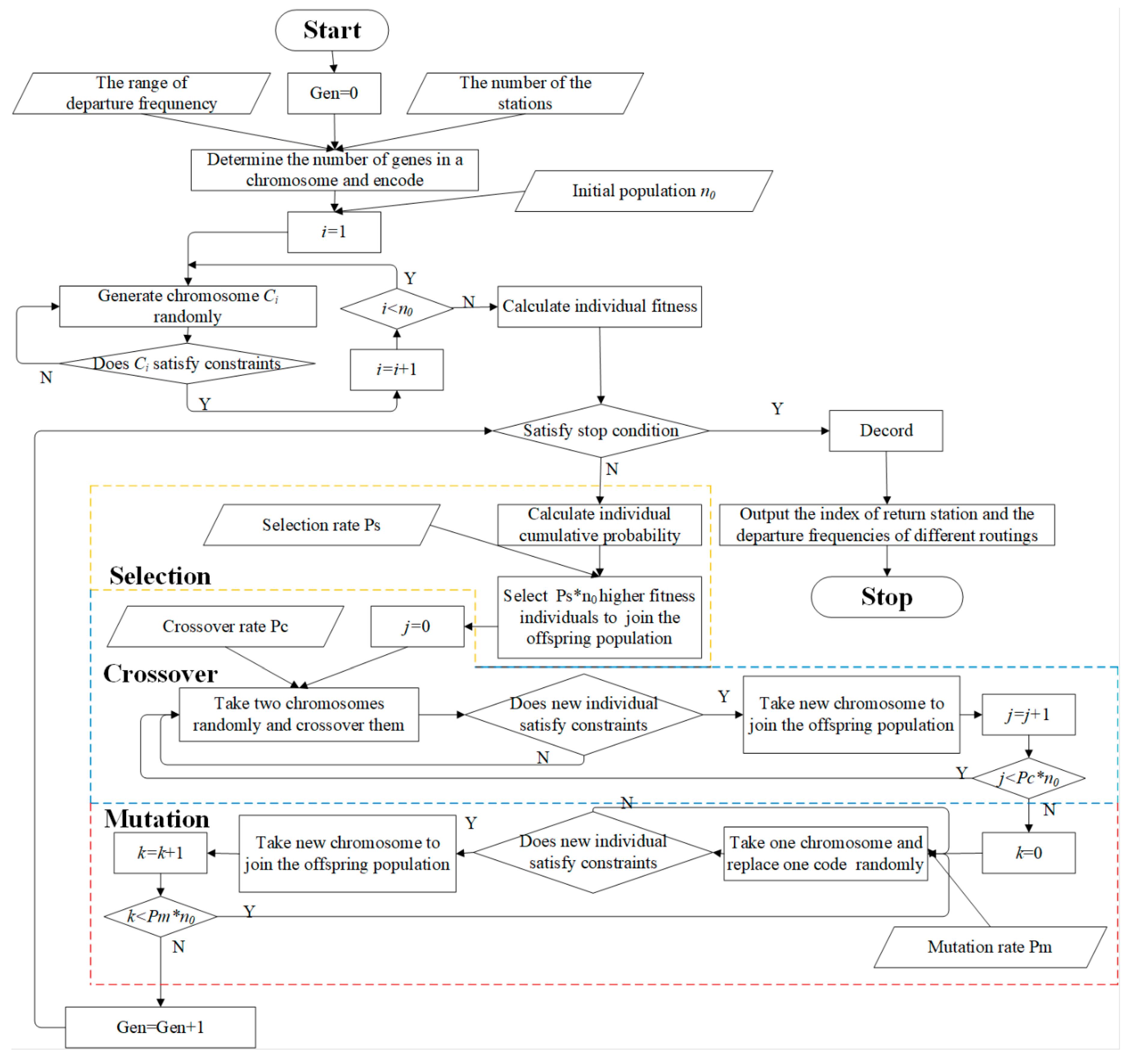Considering the actual situation of urban rail transit (e.g., multiple stations and large passenger flow), we select the CPLEX solver to try to solve the problem at first but unfortunately it takes a long time [32]. It can take up to half an hour for an optimal solution to optimize 35 stations and will be detrimental to the further development and expansion of the follow-up study. In addition, the solver does not solve the nonlinear optimization. Since with the developed double-routing optimization model it is difficult to find a good solution using the method of exhaustion or traditional optimization algorithms, we design a genetic algorithm (GA) in this study to solve the developed model, which greatly improves the solving efficiency and is more conducive to the expansion of the follow-up research. GA is a random global search algorithm and optimization method for seeking high-quality solutions. Due to its advantages of strong robustness, extensive generality and high efficiency, GA has been widely adopted for solving many urban rail optimization problems [16,33]. The basic steps of GA are coding, initial population generation, fitness evaluation, selection, crossover and mutation, as shown in Figure 4.

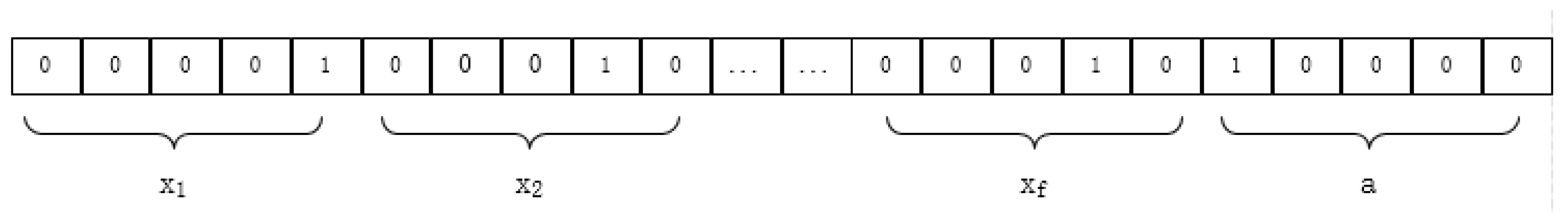
Step 1. Chromosome coding: The double-routing optimization model has f + 1 variables. The first f decision variables are the train operation plan, x₁, x₂, …, x_f; when x_i takes the value of 1, it means the train will operate on the long routing at time x_i; when the value is 2, it means the train will operate on the short routing at time x_i. The f + 1 decision variable is the index of the return station in the short routing. Therefore, the chromosome can be divided into f + 1 parts for coding, that is, one chromosome has f + 1 genes. We convert decimal variables into binary genes. In this way, a solution to the model is encoded as a solution of the GA. As shown in Figure 5, this chromosome represents that at time x₁ the train should operate on the long routing, at time x₂ the train should operate on the short routing and at time x_f the train should operate on the short routing. The index of the return station in the short routing is No.16.

Step 2. Initialization: According to the constraints of departure frequency and the return station in 18, initialize the population p₀, generate n₀ initial solutions randomly and ensure that each initial solution generated is a feasible solution.

Step 3. Evaluation function: Fitness evaluation is used to measure the quality of individual candidates. The GA is usually used to find the maximum value of the model; however, in this study we need to find the minimum value of the objective function of the double-routing optimization model. Here, we use the function f(x) = M − z(x) as the evaluation function, where M is a constant that ensures that the value of f(x) is positive. If the value of f(x) is bigger, the corresponding solution is better.

Step 4. Selection process: In this paper, the best reserved selection method is adopted. First, roulette is used for selection and then the individuals with the highest fitness in the current population are completely copied to the next generation. The cumulative probability that individual x_i is inherited to the next generation is

$$p(x_i)=f(x_i)/{\displaystyle \sum _{i=1}^{n_0}f(x_i)}$$

(21)

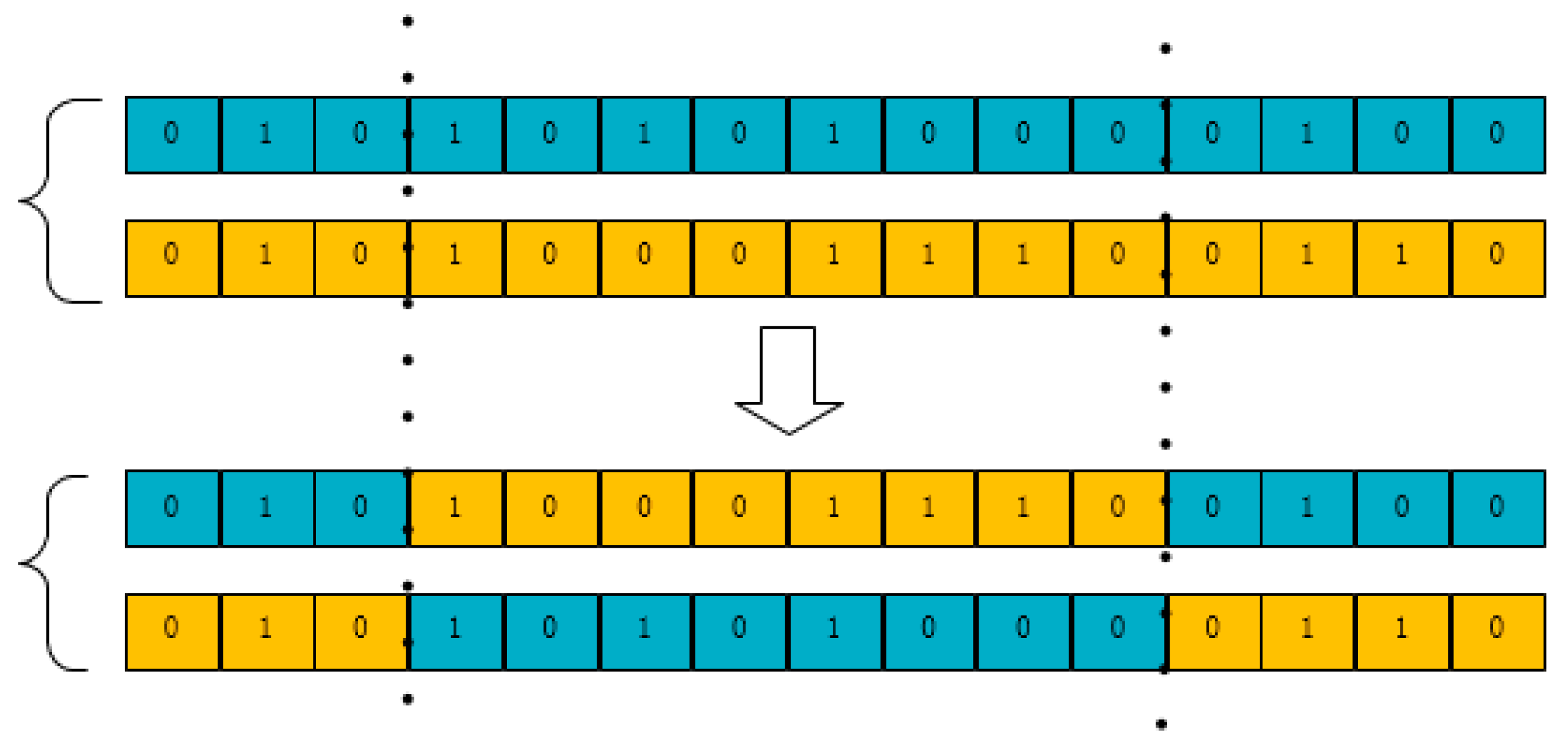
Step 5. Crossover process: The crossover is the most important step in the GA, which could generate new chromosomes in the population. This paper uses two points of crossover. First, two chromosomes are paired randomly and serve as parent chromosomes, which are selected for the new population according to the crossover probability. If the new chromosome meets all constrains, take it to replace the parent chromosome. Otherwise, keep the parent chromosome. The crossover process is shown in Figure 6.

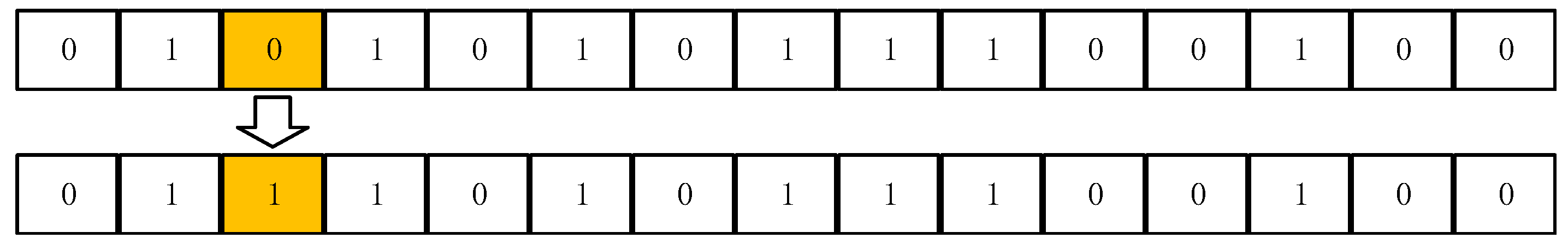
Step 6. Mutation process: The crossover process results in local optimum solutions. Thus, a mutation process is used to escape local optimums. For each chromosome in the population, we first determine whether it can be selected for the mutation operation by mutation rate. For the selected parent chromosome, randomly select a code of the chromosome. If the selected code is 0 (or 1), take 1 (or 0) to replace it. If the new chromosome meets all constrains, take it to replace the parent chromosome. Otherwise, keep the parent chromosome. The mutation process is shown in Figure 7.

6. Numerical Example

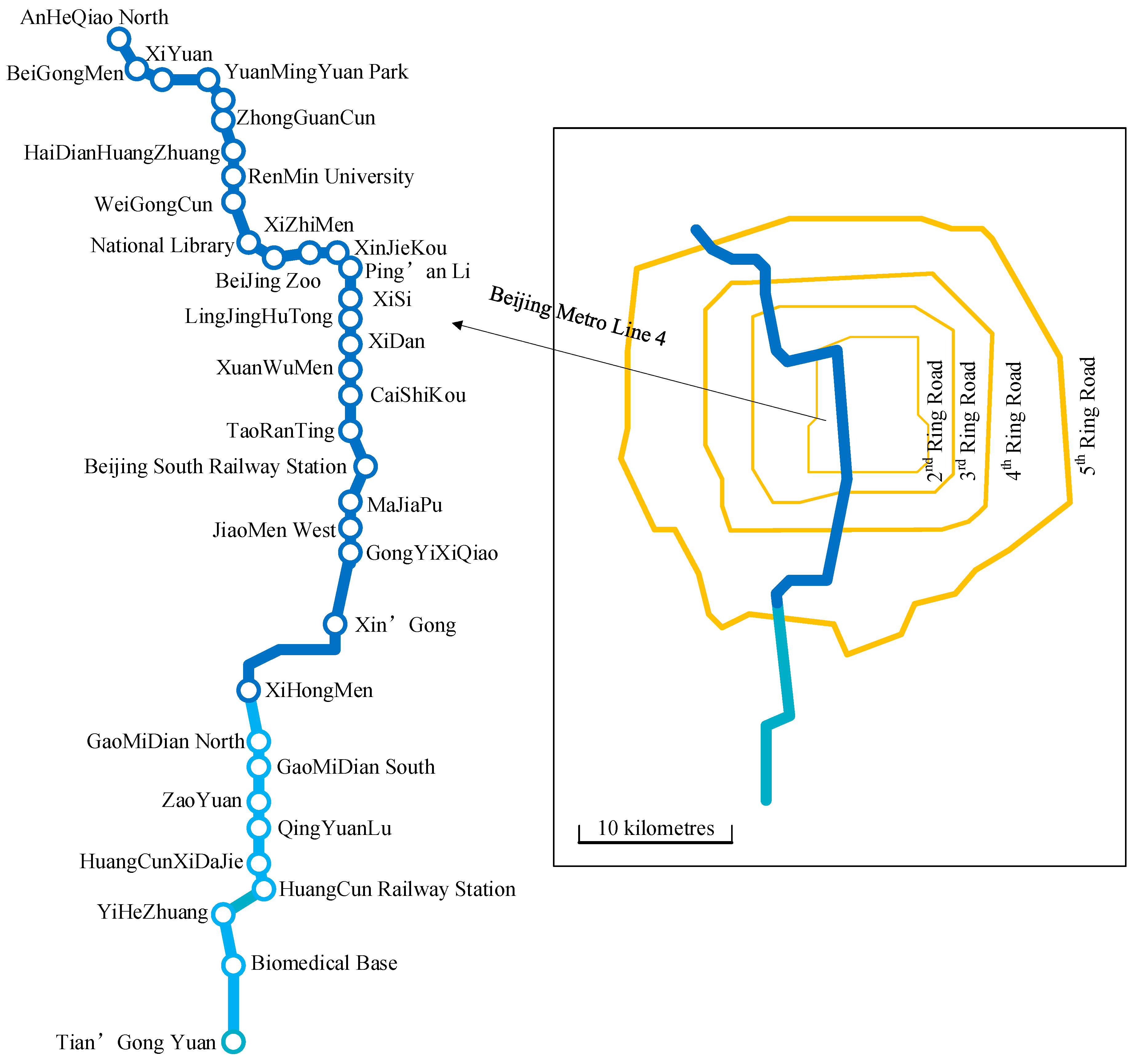
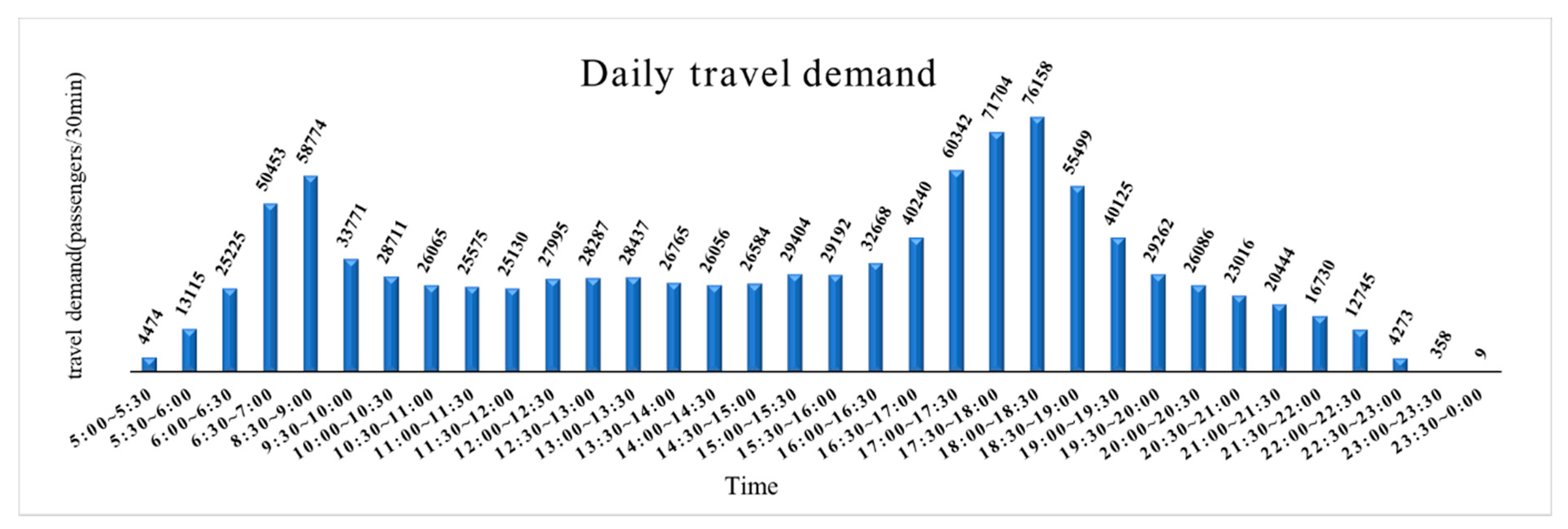
In this section, the GA is coded in Matlab programming language to verify the validity of the double-routing optimization model. This work mainly studies one direction. Beijing Metro Line 4 is a trunk line connecting the north and south areas of the western part of Beijing. We take Beijing metro line 4 as the research object, which is 50 km long and has 35 stations. First, we mark Tian’GongYuan Station as No. 1 and the Biomedical Base Station as No. 2, continuing the marking up to No. 35, in turn. The route diagram of Beijing Metro line 4 is shown in Figure 8 and the daily travel demand on line 4 is shown in Figure 9.

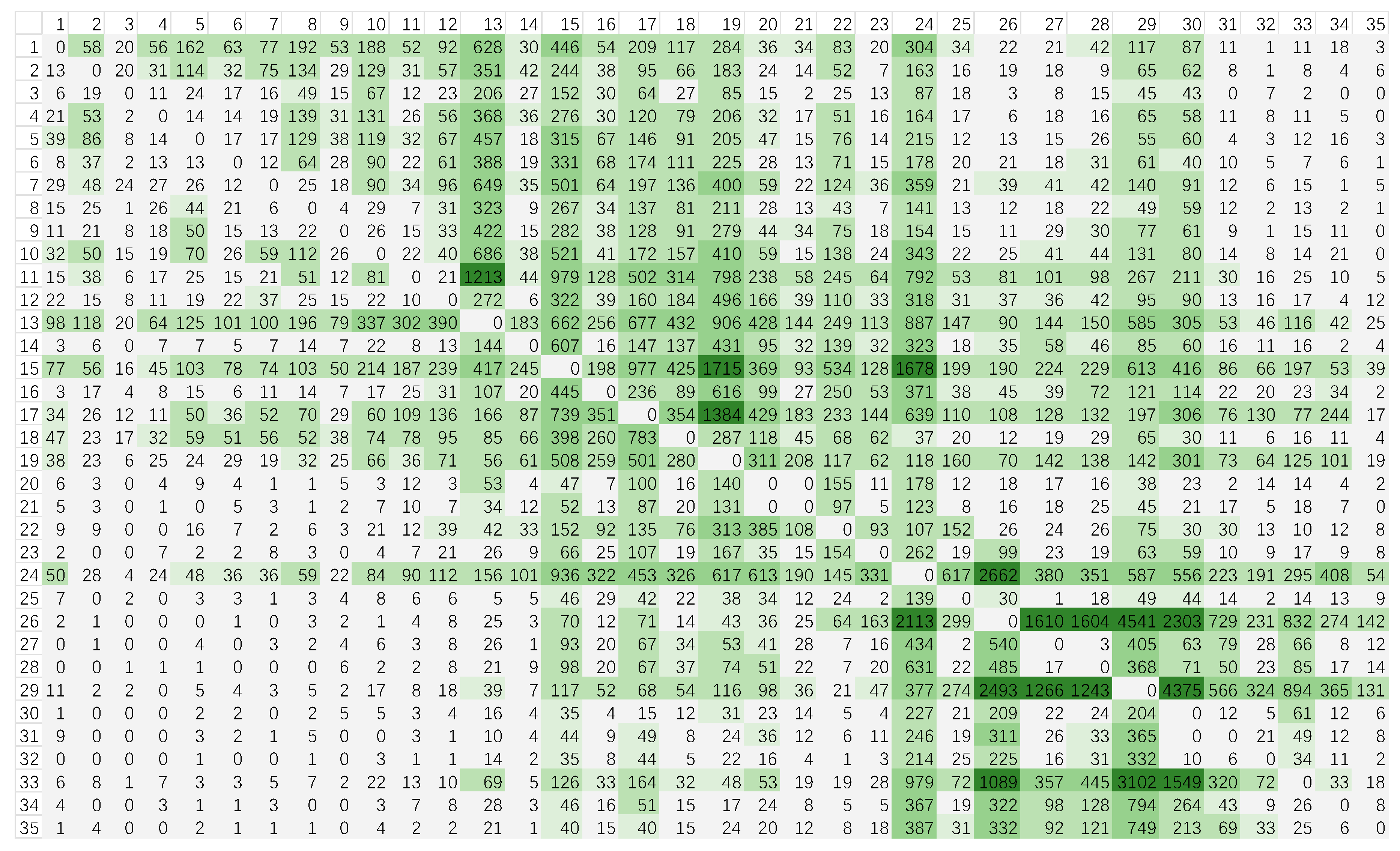
Given the OD data for Beijing metro line 4 for the whole day of 9 July 2018, this paper selects the OD data from 8:00 to 9:00 to form the OD matrix, as shown in Figure 10. The uneven distribution of OD is visually reflected by different shades of color.

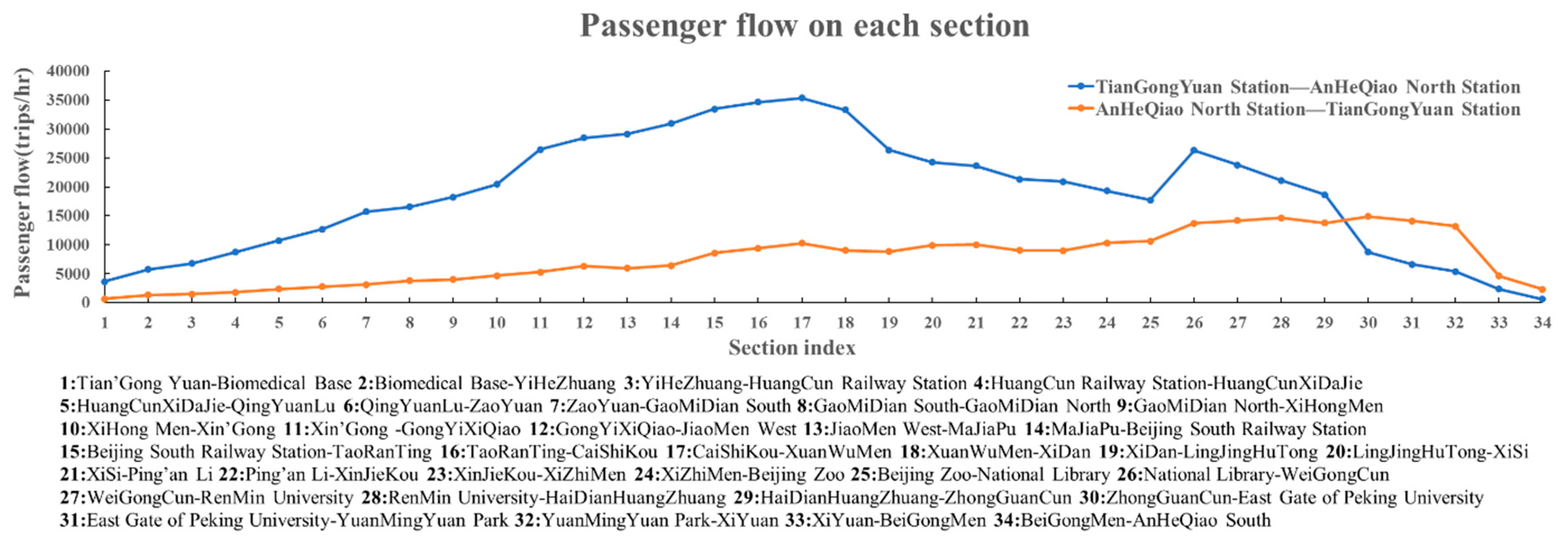
The passenger flow in each section is shown in Figure 11. During the research period, there were a total of 88,645 trips from Tian’GongYuan Station to AnHeQiao North Station and 49,681 trips from AnHeQiao North Station to Tian’GongYuan Station. The uneven passenger flow distribution in both directions is caused by the large number of morning commuters from the suburbs to the city. We choose the direction with high passenger flow from Tian’GongYuan Station to AnHeQiao North Station as the optimization target. It can be seen from Figure 10 that the maximum passenger flow is from CaiShiKou Station to XuanWuMen Station—in this section there were 35,391 passengers bound for AnHeQiao North Station and 10,273 passengers bound for Tian’GongYuan Station. For this reason, we choose [a, n] as the short routing.

According to the code for the design of the metro and combining the actual operation characteristics of the metro systems, the equipment operating data and some parameters in the model are shown in

Table 2. Equipment operating data and some parameters for Line 4.

Parameters	I0	tz	tz′	fmin	Cz	α	n	f
Value	120 s	150 s	180 s	12 tr/h	1460	100%	35	24

.

This paper implements GA with Matlab programming to optimize the double-routing optimization model. The relevant parameters of the GA are shown in

Table 3. Values of GA parameters.

Parameters	Maximum Number of Iterations	Initial Population Size	Crossover Rate	Mutation Rate
Value	100	100	0.9	0.05

.

When the objective is to minimize passenger waiting time, the decision variables are obtained as shown in

Table 4. Values of decision variables when taking passenger waiting time as the objective.

Decision Variables	1	2	3	4	5	6	7	8	9	10	11	12	13
Value	1	1	1	1	1	1	1	1	1	1	1	1	1
Decision Variables	14	15	16	17	18	19	20	21	22	23	24	25
Value	1	1	1	1	1	1	1	1	1	1	1	2

, which indicates that all trains should run on the long routing; at the same time this will cause a certain wasted capacity. When the objective is to minimize the wasted capacity, the decision variables are received as shown in

Table 5. Values of decision variables when taking wasted capacity as the objective.

Decision Variables	1	2	3	4	5	6	7	8	9	10	11	12	13
Value	1	2	2	1	1	2	2	2	1	2	2	2	2
Decision Variables	14	15	16	17	18	19	20	21	22	23	24	25
Value	1	2	2	2	2	1	1	2	1	1	2	26

, indicating that there are 15 trains running on the short routing and 9 trains on the long routing in an hour; this will cause the minimum wasted capacity and a greater passenger waiting time. A specific comparison of the effects on different objective functions is shown in

Table 6. Comparisons of the effects on different objective functions.

	Taking Passenger Waiting Time as the Objective Function	Taking Wasted Capacity as the Objective Function
Departure frequency	24 tr/h, where 24 tr/h are on the long routing	24 tr/h, where 10 tr/h are on the long routing and 14 tr/h are on the short routing [28,35]
Total waiting time for passengers	110,810	252,680
Wasted capacity	60,825	118
Total objective function	171,630	252,798

.

It can be seen that taking passenger waiting time or wasted capacity as the objective function is not enough, since this will either cause a certain wasted capacity or seriously affect the service quality. Therefore, the objective function combining passenger waiting time and wasted capacity is very necessary.

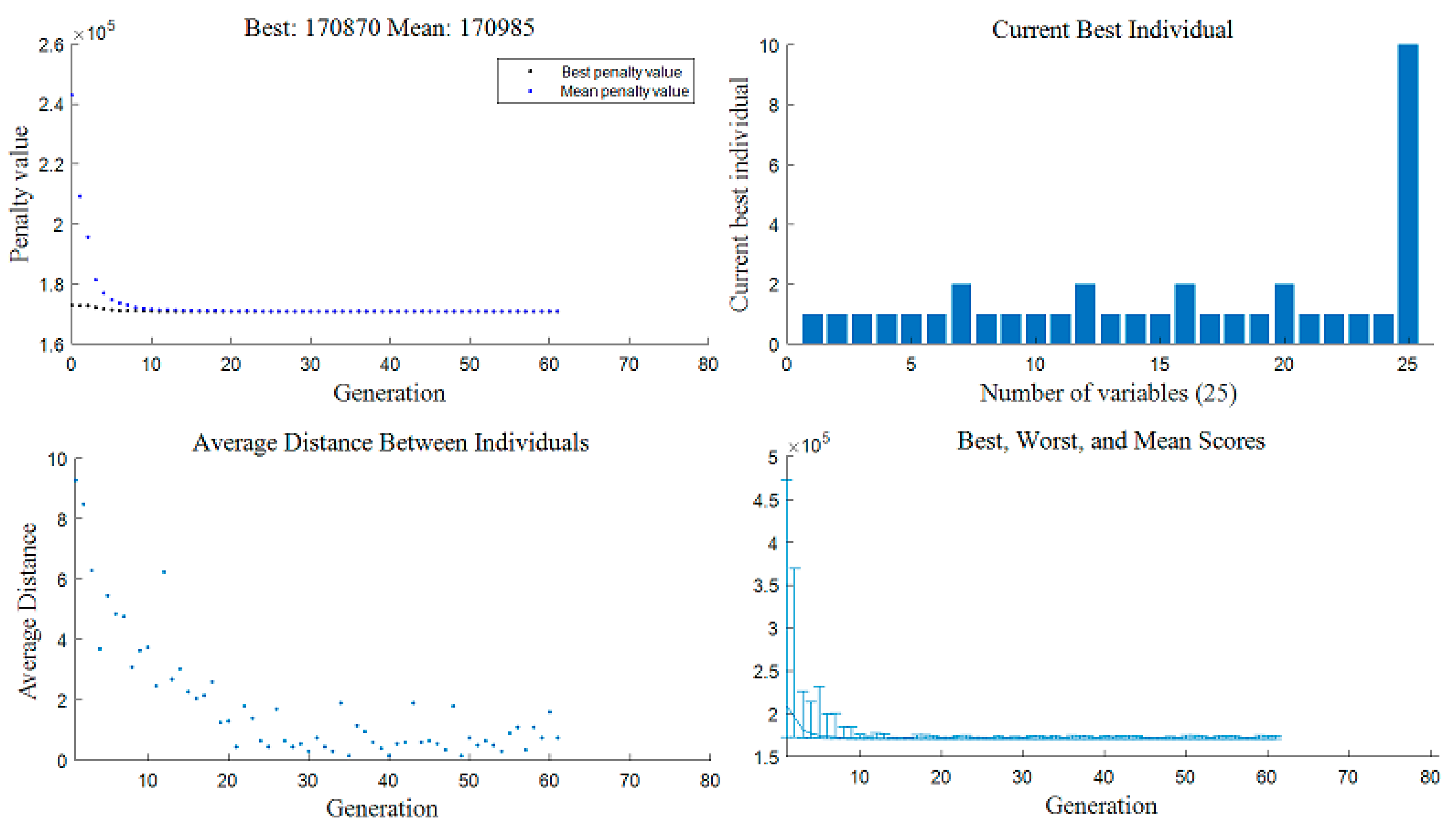
We substitute the parameters into the double-routing model and find the solution. The variation tendencies of average fitness, optimal fitness, the average distance between individuals and scores in the iteration process of the genetic algorithm are shown in Figure 11 and thus we obtain the current best individual.

It can be observed from Figure 12 that in the iteration process of the genetic algorithm, the average fitness and the optimal fitness show a downward trend and so do the scores and average distance between individuals. The variation tendencies of average fitness and optimal fitness show that the algorithm has good convergence. When the objective function takes the minimum value, the values of the decision variables are as shown in

Table 7. Values of decision variables with the objective function combining passenger waiting time and wasted capacity.

Decision Variables	1	2	3	4	5	6	7	8	9	10	11	12	13
Value	1	1	1	1	1	1	2	1	1	1	1	2	1
Decision Variables	14	15	16	17	18	19	20	21	22	23	24	25
Value	1	1	2	1	1	1	2	1	1	1	1	10

. The index of the return station in the short routing is No. 10, namely XiHongMen Station. The short routing is [XiHongMen Station, AnHeQiao North Station].

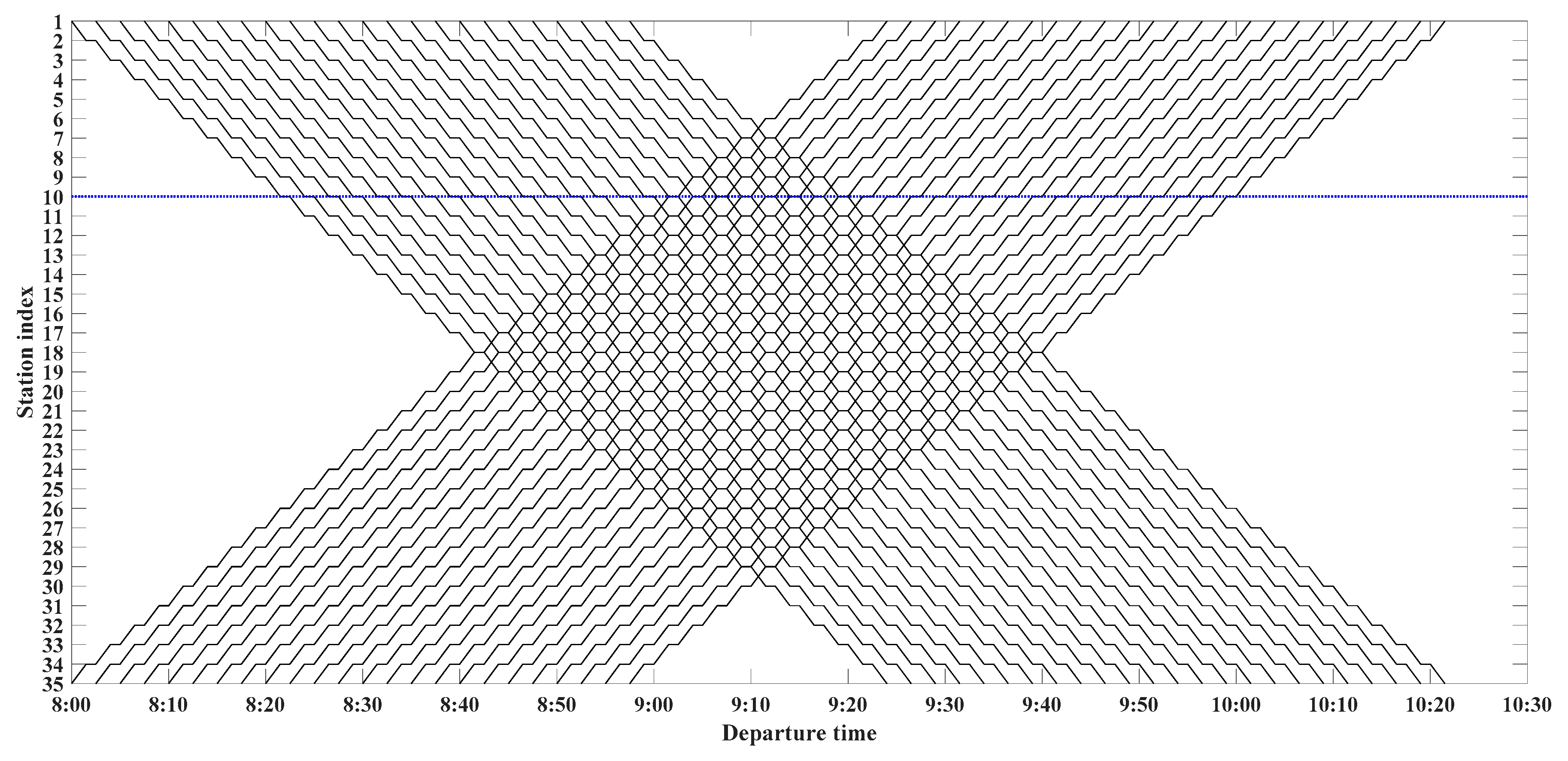
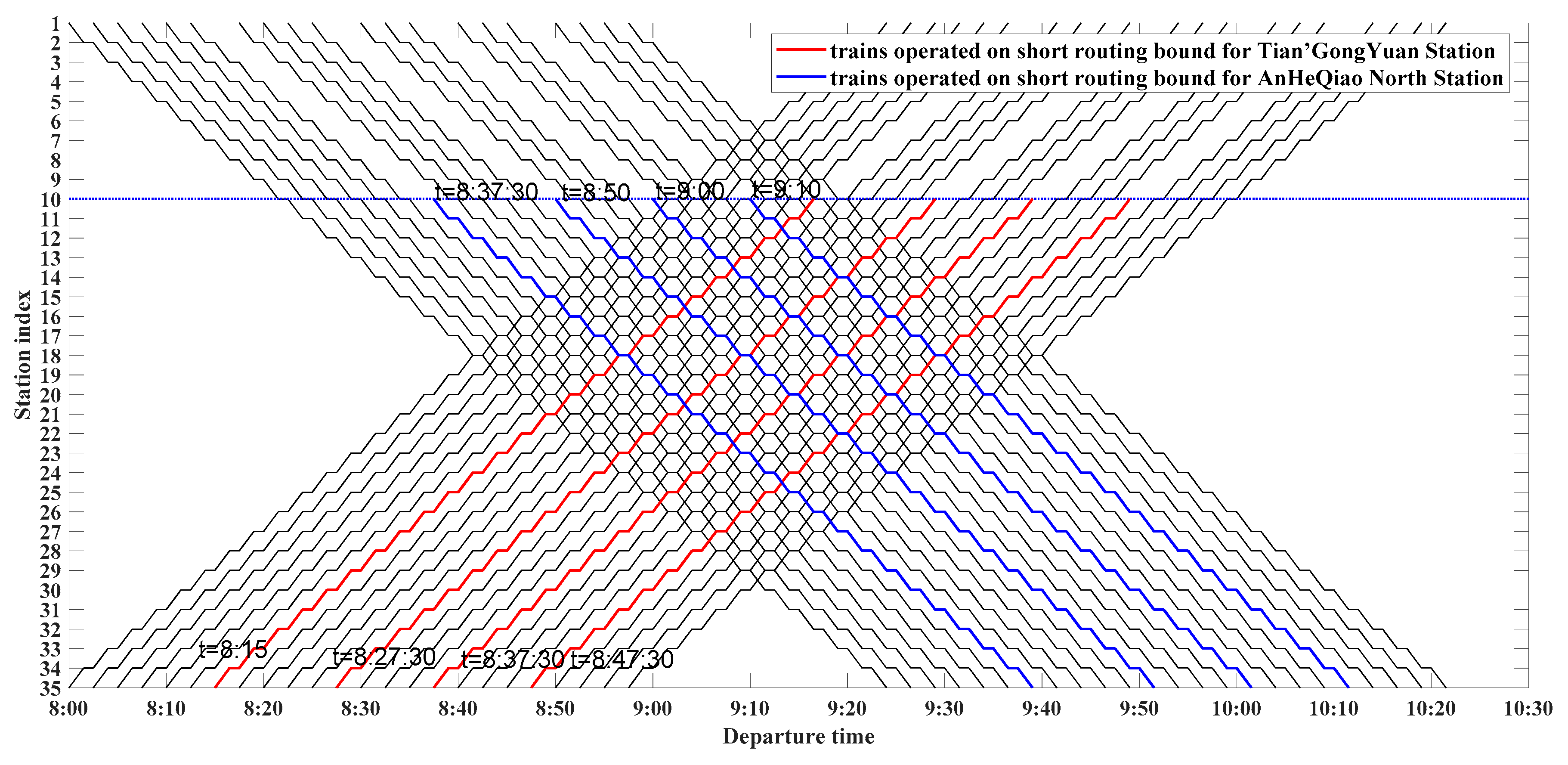
The train timetables before and after optimization are shown in Figure 13; Figure 14. The x-coordinate indicates the departure times of trains and the y-coordinate indicates the stations along Metro Line 4. It can be seen from Figure 13 and Figure 14 that for trains operated on balanced scheduling mode, every 2.5 min a train will be sent from AnHeQiao North Station and Tian’Gong Yuan Station. The blue line parallel to the X-axis in Figure 14 represents XiHongMen Station, which is the turn-back station of the short routing.

In Figure 14, there are four trains that turn back at XiHongMen Station; the rest of trains are operated on the same timetable as before the optimization. We compared the effects before and after optimization obtained by using the double-routing optimization model and the specific contents are shown in

Table 8. Comparison of effects before and after Optimization.

	Before Optimization	After Optimization
Operation mode	Single long routing	Mixed operation on long and short routings
Departure frequency	24 tr/h	24 tr/h, where the long routing has 20 tr/h and the short routing has 4 tr/h
Train operation plan	The trains run every 150 s from 8:00 to 9:00. Each train is operated on long routing	The trains run every 150 s from 8:00 to 9:00. At 8:15, 8:27:30, 8:37:30 and 8:47:30, trains will be operated on the short routing and at the rest of the time trains will be operated on the long routing
Total waiting time for passengers	110,810	115,830
Wasted capacity	60,825	55,043
Total objective function	171,630	170,873

.

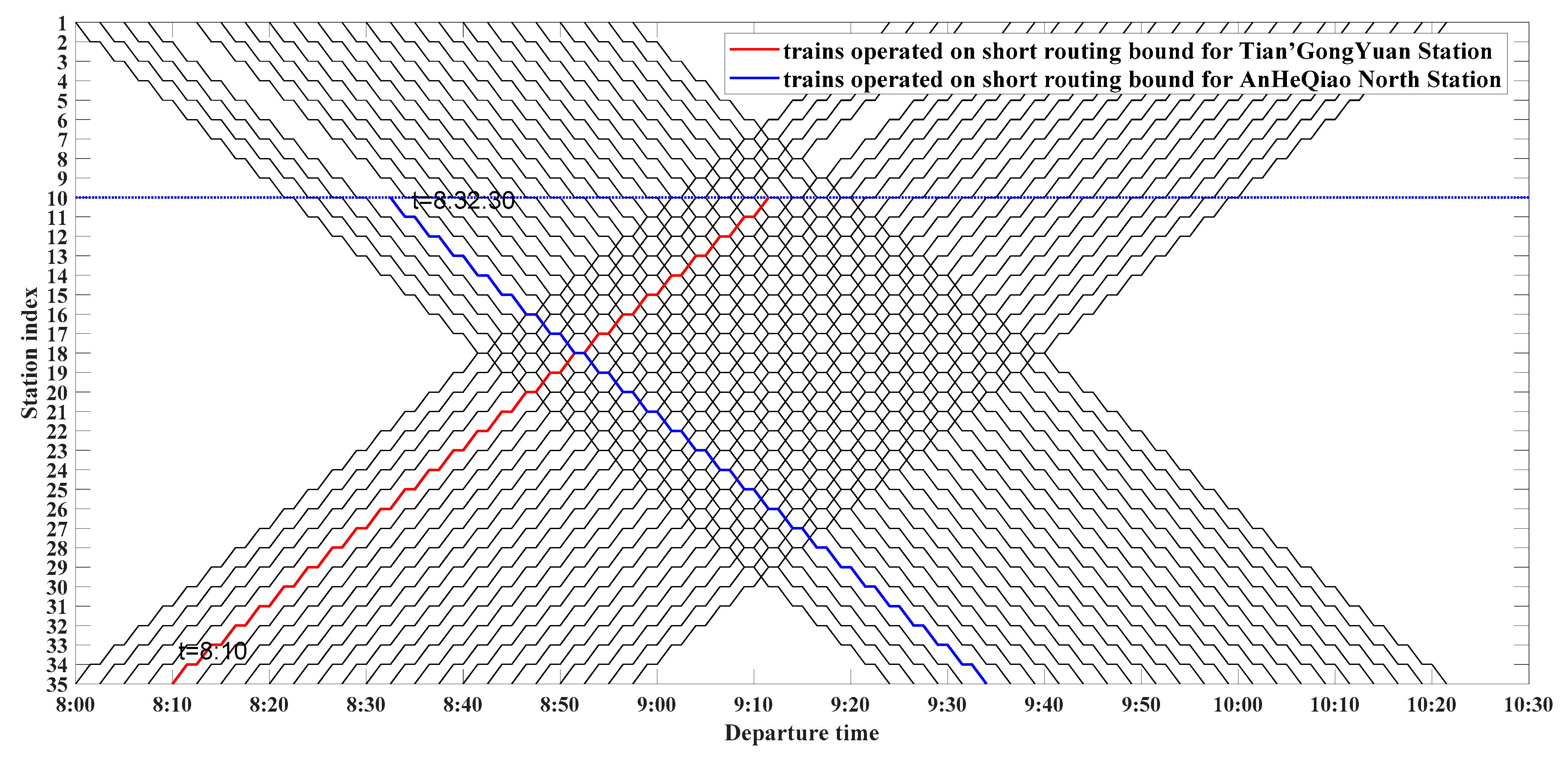
It can be observed from Figure 13, Figure 14 and Table 8 that the wasted capacity of Beijing Metro Line 4 decreased by 9.5% with the optimized train operation plan, while the passenger waiting time increased by 4.5%, which can verify that this optimization model is very effective. We take the passenger flow in two directions into consideration and substitute them into the model to obtain the result, as shown in

Table 9. Values of decision variables when taking two directions into account.

Decision Variables	1	2	3	4	5	6	7	8	9	10	11	12	13
Value	1	1	1	1	2	1	1	1	1	1	1	1	1
Decision Variables	14	15	16	17	18	19	20	21	22	23	24	25
Value	1	1	1	1	1	1	1	1	1	1	1	10

. In the best found train timetable, as shown in Figure 15, there is one train that turns back at XiHongMen Station, while the rest of trains are operated the same as before the optimization.

As can be seen from Table 9, when two directions are taken into consideration, the index of the return station does not change but the departure frequency on the short routing decreases and on the long routing it increases accordingly.

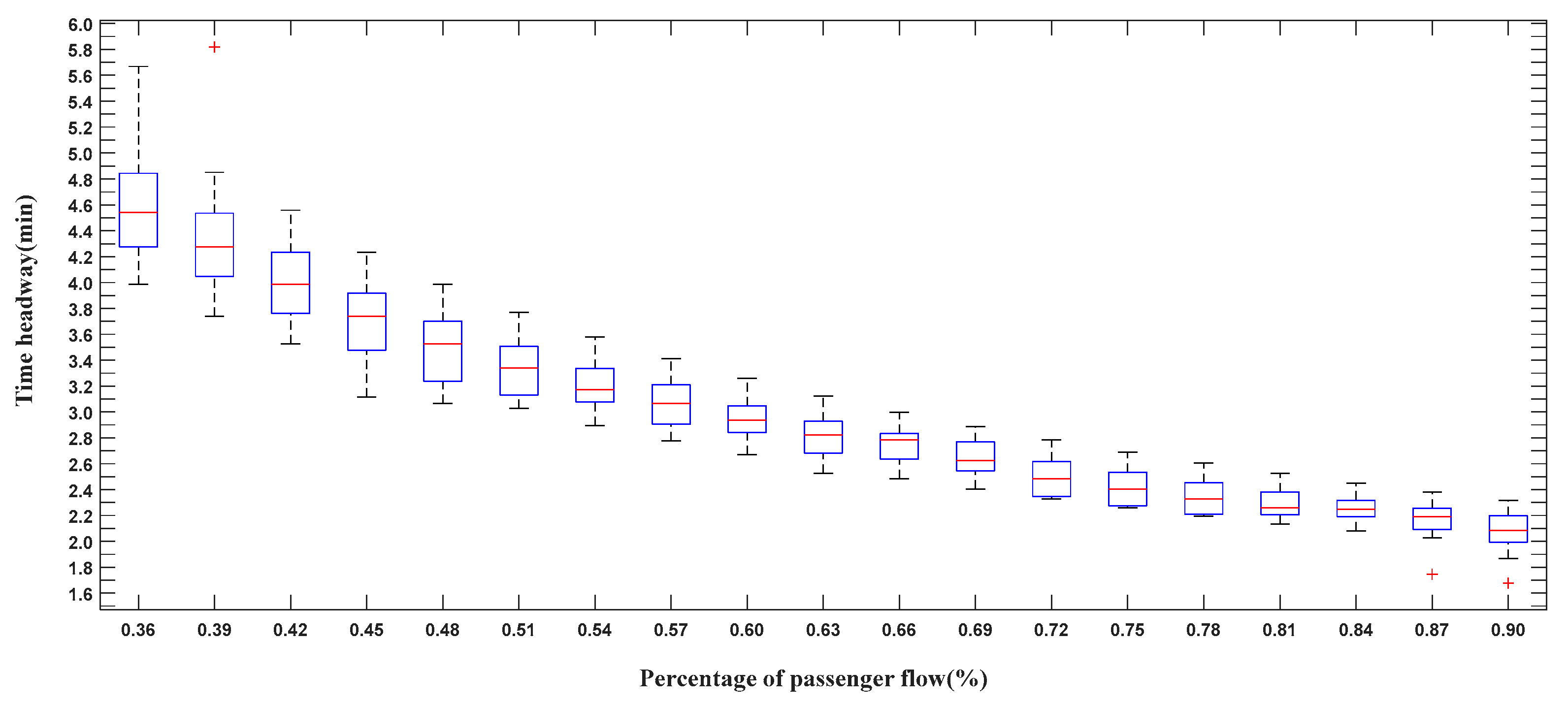
The departure frequency on a single long routing can be calculated by the maximum section passenger flow, which is our consensus. Through the in-depth study of this model, we obtain the relationship between the total passenger flow and trains’ optimum headway, which makes it unnecessary to calculate the section passenger flow and find out the maximum section passenger flow specifically. To some extent, this facilitates our calculation. As shown in Figure 16, the horizontal axis is the ratio of the total passenger flow to the maximum passenger flow; the maximum passenger flow here is calculated according to the maximum train operated on the single long routing and the load factor is 130%. The vertical axis is the optimal headway.

The following part will simulate some different compromise solutions and study some influencing factors of the model, such as the location of the return station in the short routing, the number of trains on the short routing, the ratio of passenger flow in the short routing and the upper limit of the load factor, in the hope of reaching recommendations for metro trains operated on the double routings.

The location of the short routing’s return station will affect the ratio of passenger flow and the short routing’s turnover time, which will have an impact on the optimal train routing plan and the passengers’ total waiting time. We set other variables as fixed and change the index of the return station. The optimal train routing plan and the influence of the return station’s location are shown in

Table 10. The optimal train routing plan and influence of the turn-back station’s location on optimal routing plans.

	Short Routing		Departure Frequency (tr/h)		The Optimization Effect
	Origin Station	Terminal Station	Long Routing	Short Routing	Total Passenger Waiting Time	Wasted Capacity	Combining Cost
1	35	8	21	3	113,770	57,452	171,222
2	35	9	21	3	114,050	56,971	171,021
3	35	10	20	4	115,830	55,043	170,865
4	35	11	21	3	114,940	56,007	170,947
5	35	12	22	2	114,150	57,292	171,442
6	30	10	20	4	117,988	51,831	169,810
7	31	10	20	4	117,460	52,474	169,930
8	32	10	20	4	117,140	53,116	170,260
9	33	10	19	5	118,150	51,992	170,142
10	34	10	20	4	115,960	54,401	170,360

.

From Table 10, it can be seen that the departure frequency on long and short routings changed when the location of the turn-back station moved. When the short routing is [10,35], the departure frequency on the short routing is 4 tr/h; at this point, we select h = 35 as the origin station and fix it, moving the terminal outwards or inwards and the frequency on the short routing reduces. When the short routing is [10,33], the departure frequency on the short routing is 5 tr/h; we select h = 10 as the terminal and fix it; when the origin station is moved outwards or inwards, the frequency on the short routing reduces. It can be found that when the short routing is [10,30] and the short routing’s departure frequency is 4 tr/h, the combined cost is at the minimum but at this time, there are two stations that need to be reconstructed. If we intend on achieving the optimization purpose by reconstructing only one station, the optimal routing plan is [10,35] and the departure frequency on the short routing is 4 tr/h.

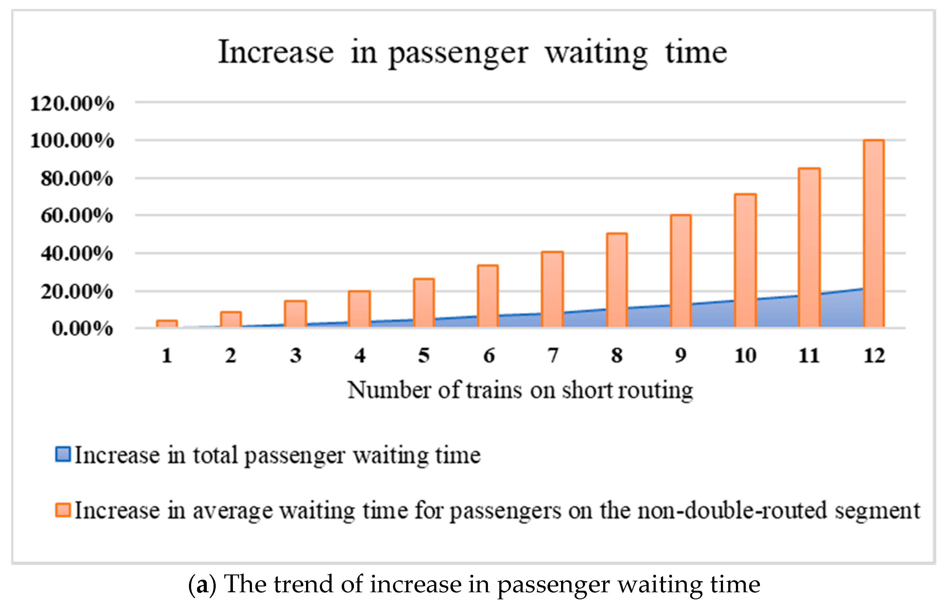
When the short routing is fixed, the proportion of trains on the short routing will directly affect the passenger’s total waiting time.

Table 11. Impact of the different proportion of trains.

Number of Trains on the Short Routing	Total Passenger Waiting Time	The Average Waiting Time for Passengers on the Non-Double-Routed Section	Increase in Average Waiting Time for Passengers on the Non-Double-Routed Section
1	111,900	1.30	4.00%
2	113,090	1.36	8.80%
3	114,390	1.43	14.40%
4	115,830	1.50	20.00%
5	117,410	1.58	26.40%
6	119,170	1.67	33.60%
7	121,140	1.76	40.80%
8	123,360	1.88	50.40%
9	125,867	2.00	60.00%
10	128,740	2.14	71.20%
11	132,050	2.31	84.80%
12	135,910	2.5	100.00%

and Figure 16 show the impact of the different train proportions on passenger waiting time. At this time, the total number of trains is 24 and the short routing is [10,35].

The service level is closely related to passenger waiting time. From Table 11 and Figure 17, it can be seen that the total passenger waiting time increases, with the number of trains on the short routing increased. In order to ensure the service quality, the number of trains on the short routing cannot be too many. Therefore, we can determine the maximum number of trains on the short routing based on the service quality requirements of the metro operation company.

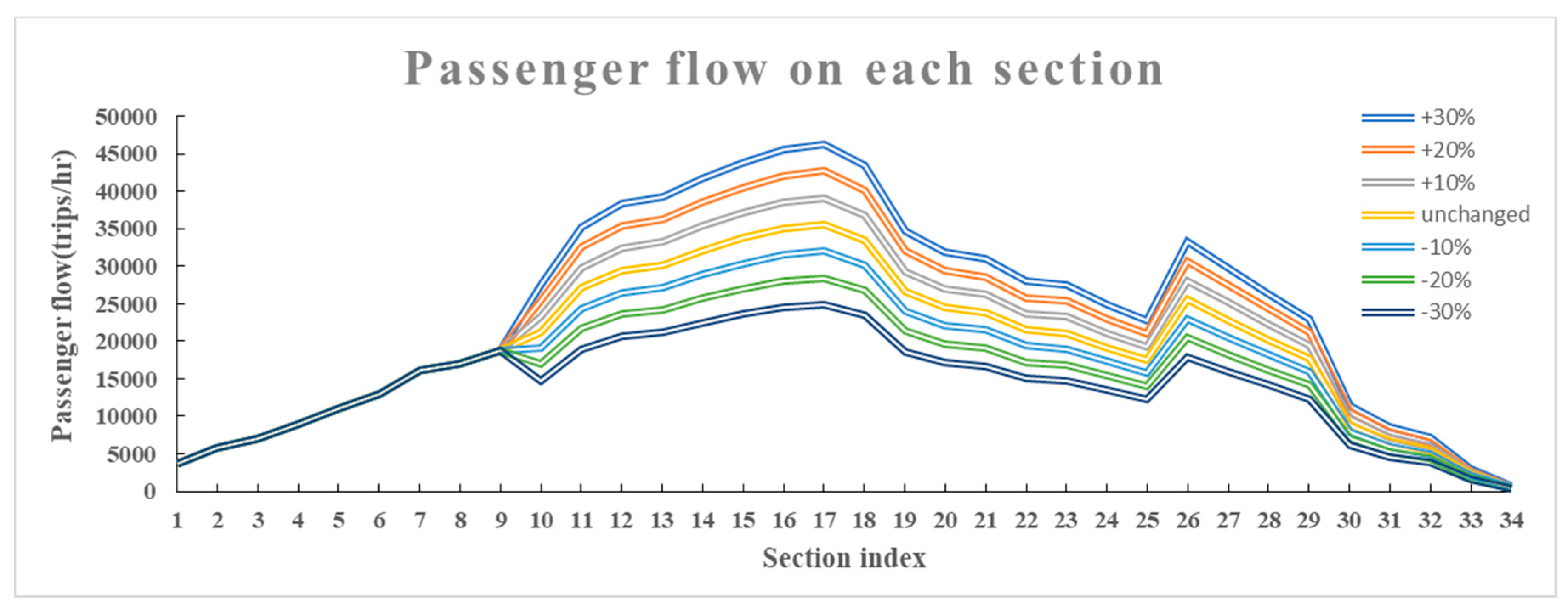
The passenger flow in the short routing refers to the flow of passengers whose origin and destination are both within the short routing, that is, In this case study, O ∈ [10,35] and D ∈ [10,35]. In order to study the influence of the ratio of the short routing’s passenger flow, the original data are processed by increasing or decreasing the passenger flow in [10,35] by 10% ,20% or 30%, successively. The different passenger flow distribution patterns are shown in Figure 18, which are +30%, +20%, +10%, −10%, −20% and −30% different from the original passenger flow, respectively. The optimal train routing plans under different passenger flow conditions are shown in

Table 12. The optimal train routing plans under different passenger flow conditions.

Magnitude of Change	+30%	+20%	+10%	0	−10%	−20%	30%
The Proportion of Passenger Flow in [10,35]	81.6%	80.4%	78.9%	77.3%	75.4%	73.2%	70.5%
Deviation from the Average Section Passenger Flow	+11.6%	+10.4%	+8.9%	+7.3%	+5.4%	+3.2%	+0.5%
Short Routing	[1,34]	[1,34]	[1,34]	[10,35]	[2,35]	[2,35]	[2,35]
Departure Frequency on the Long Routing	25	24	23	20	22	20	18
Departure Frequency on the Short Routing	5	6	4	4	0	0	0

.

By changing the passenger volume, it can be found that when the passenger flow in [10,35] is increased, the departure frequency is first determined according to the maximum section passenger flow and then the short routing with higher passenger flow is re-selected to complete optimization. When the passenger flow increases by 10%, the departure frequency increases to 27 tr/h. The departure frequency cannot keep increasing, due to the constraints of safe operation and the signal system, therefore, when the passenger flow increases by 20% or even 30%, it is determined as 30 tr/h. When the passenger flows in [10,35] are decreased by 10% and 20%, the volumes in the short routing are only 5.4% and 3.2% higher than the average section passenger volume. The optimal train routing plans obtained by the model are the same as the single long routing, indicating that in these cases, metro trains are not suitable for operating on the double routing. When the passenger flow in [10,35] decreases by 30%, the passenger flow of each section is basically the same. The wasted capacity caused by the single long routing will be relatively low and the requirement can be satisfied by trains operated on the single long routing. Therefore, we infer that when there are some sections whose passenger flow is more than 6% higher than the average section passenger flow, the double routing model can be considered.

The change in the upper limit of the load factor will directly affect the value range of feasible solutions. In

Table 13. The optimal train routing plans under different load factors.

The Upper Limit of the Load Factor	Short Routing	Departure Frequency on the Long Routing	Departure Frequency on the Short Routing
80%	[1,34]	24	1
90%	[10,35]	22	2
100%	[10,35]	20	4
110%	[10,35]	19	5
120%	[1,34]	20	4

, the optimal train routing plans under different load factors are shown.

The upper limit of the load factor will affect the passenger waiting time and the train departure frequency. When the load factor declines, the capacity of each train will decrease and passenger flow can be satisfied by increasing the departure frequency. With the increase of the load factor, the departure frequency on the short routing increases, while the frequency on the long routing decreases correspondingly. The reduction of the departure frequency on the long routing will reduce the waste of transportation capacity but at the same time will lead to the increase of passenger waiting time on non-double-routed sections, which is a mutual restriction process. When the upper limit of the load factor is 120%, the obtained short routing is very close to the complete long routing. The above experimental results basically agree with the theoretical analysis and the actual situation, which validates the feasibility of the optimization model.

7. Conclusions

According to the characteristics of the mixed operation on long and short routings, we develop a nonlinear integer optimization model to reduce both passenger waiting time and wasted capacity on the balanced scheduling mode. A genetic algorithm was used to solve the problem. Finally, we take the passenger data and operation data of Beijing Metro Line 4 as a numerical example. The train operation plan was optimized so that the wasted capacity decreased by 9.5%, in addition, the total objective function value decreases by 0.45% when the passenger waiting time increases by 4.5%, which can verify that this optimization model is very effective.

The work presented in this paper is by no means complete and further research is needed in the following directions. First, for the convenience of modeling, the departure frequency after optimization is the same as when the trains operated on the single long routing and for this reason, the passenger waiting time increases a little. In fact, when ensuring that the number of trains used does not increase and when considering the differences in the turnover times of the double routings, the departure frequency can increase, so that it can make passenger waiting time decrease and not affect transport enterprises’ interests. Second, the model in this paper is established based on the real-time information from smart cards. The real-time performance should be explored by improving the algorithm, so as to generate more accurate schemes to guide the mixed operation on long and short routings. Faster algorithms need to be developed to solve large size problems. Lastly, further research will take the actual conditions of each station into account and consider the influence of different train types and formations on the double routing optimization model.