Agriculture Sprawl Assessment Using Multi-Temporal Remote Sensing Images and Its Environmental Impact; Al-Jouf, KSA

Abstract

In this paper, multispectral and multi-temporal satellite data were used to assess the spatial and temporal evolution of the agriculture activities in the Al-Jouf region, Kingdom of Saudi Arabia (KSA). In the current study, an attempt was made to map the agriculture sprawl from 1987 to 2017 using temporal Landsat images in a geographic information system (GIS) environment for better decision-making and sustainable agriculture expansion. Our findings indicated that the agriculture activities developed through two crucial stages: high and low rise stages. Low rise stages occurred during three sub-stages from April 1987 to April 1988, from September 1993 to August 1998, and from April 2008 to May 2015, with overall change rates of 37.9, 44.4, and 30.5 km²/year, respectively. High rise stages occurred during three sub-stages from April 1988 to February 1993, from September 2000 to March 2006, and from April 2016 to August 2017, with overall change rates of 132.4, 159.1, and 119.5 km²/year, respectively. Different environmental problems due to uncontrolled agriculture activities were observed in the area, including substantial depletion of the groundwater table. Another environmental impact observed was the appearance of sinkholes that occurred suddenly with no warning signs. These environmental impacts will increase in the future if no regulated restrictions are implemented by decision-makers.

1. Introduction

Agriculture areas in most communities throughout history have played a vivid role in many countries’ prosperity [1]. Both developed and undeveloped countries are relying on agriculture for economic as well as food security [2]. Agriculture is a primary source for developing the economy. In many areas, human demands for food and accommodation have increased over time due to the increase in human population [3]. However, these agriculture expansions have significantly changed the natural landscape, leading to immense environmental impacts [4].

The unplanned and uncontrolled rapid growth in agriculture activities, particularly in developing countries, relies entirely on fossil water, which might lead to severe negative environmental impacts [5]. These impacts include intensive use of groundwater, which applies massive pressure on aquifer productivity due to over abstraction and depletion of the water table in many regions [6]. The intensive use of groundwater has caused severe depletion of the water table up to 2–3 m/yr in Baluchistan, Pakistan [7], and 1 m/yr in the Egyptian west Delta aquifer [8]. Significant drops in groundwater levels have been observed for many areas (e.g., the Beijing Plain, China, up to 20 m total drop since 1970 [9]; in the Beqaa valley, Lebanon, up to 40 m between 1970 and 2010 [10]). The excessive use of groundwater resources may also lead to a wide spectrum of social, economic and environmental consequences, such as, the drop in water level, the loss of water resources, and the appearance of sinkholes in some areas [11,12].

Remote sensing (RS) and geographical information systems (GIS) are very effective techniques for analyzing time series data, in addition to being cost-effective methods that can be applied to cover large areas [13,14,15,16,17]. Remote sensing data include satellite, radar, and light detection and ranging (LiDAR) data, as well as aerial photos that are acquired from different platforms, such as unmanned devices, airplanes, and space-borne satellites. The temporal analysis of satellite images can provide vital data on urban sprawl, agriculture dynamics, and land use changes, which can be determined using several modeling techniques [18,19,20,21,22,23,24,25].

Many studies have used advanced techniques in satellite image analysis to map agriculture and crop areas [26,27,28,29,30,31,32,33,34]. One such favorite technique is the normalized difference vegetation index (NDVI), which has been utilized for monitoring cropland and land use/land cover (LULC) changes over various time series [35,36,37,38,39,40]. However, NDVI can be influenced by many factors (e.g., soil exposure characteristics, the topography of the area, the senescence and density of vegetation, atmospheric pollutions, surface albedo, sun elevation angle, and the moisture content of exposed soil) [41,42]. Another technique, supervised classification, is widely used to derive land cover types, deforestation, fire detection, and crop production, as well as to monitor environmental pollution [43,44]. The supervised classification method uses many algorithms, including parallel pipeline, the maximum likelihood method, fuzzy-rule based techniques, artificial neural networks, and support vector machines [45,46].

Desert agriculture is quite booming in Saudi Arabia, which started in the 1960s with a total cultivated area of 3400 km² and increased to 34,218.54 km² in 2017 [47]. According to Ouda [48], this type of agriculture activity was encouraged by the government to achieve food self-sufficiency. Groundwater is the main source for irrigation (up to 97% of irrigation water comes from groundwater resource) [49]. The Al-Jouf region is one of the agriculture areas in Saudi Arabia. It is characterized by Sirhan Formation, which is composed of limestone rocks. This formation is prone to sinkhole development through dissolution by water [11,12]. Since 2010, there have been many sinkholes reported in the Al-Jouf area. The occurrence of sinkholes can threaten the environment and cause severe damage to the area [50]. Many authors have reported that the phenomena of land subsidence and sinkholes are the result of groundwater extraction for agricultural and industrial use [5,11,12,51,52,53,54].

Due to the unexpected acceleration of agriculture activities in the Al-Jouf area, there is an urgent interest in understanding their development over time and their environmental impacts. Accordingly, the main objectives of this study were to monitor agriculture changes in the Al-Jouf region over a period of ~31 years, from 1987 to 2017, and thereby capture and determine the environmental impact of agriculture sprawl (the impact of agriculture expansion on groundwater level drop and the occurrence of different types of sinkholes in the area).

The current work represents a crucial method for connecting changes in agriculture activities with the environmental problems in the area, which will help decision-makers to identify the amount of groundwater that is exploited from the aquifer, anticipate the future changes in the groundwater level, and take appropriate action to minimize or prevent any future environmental impacts.

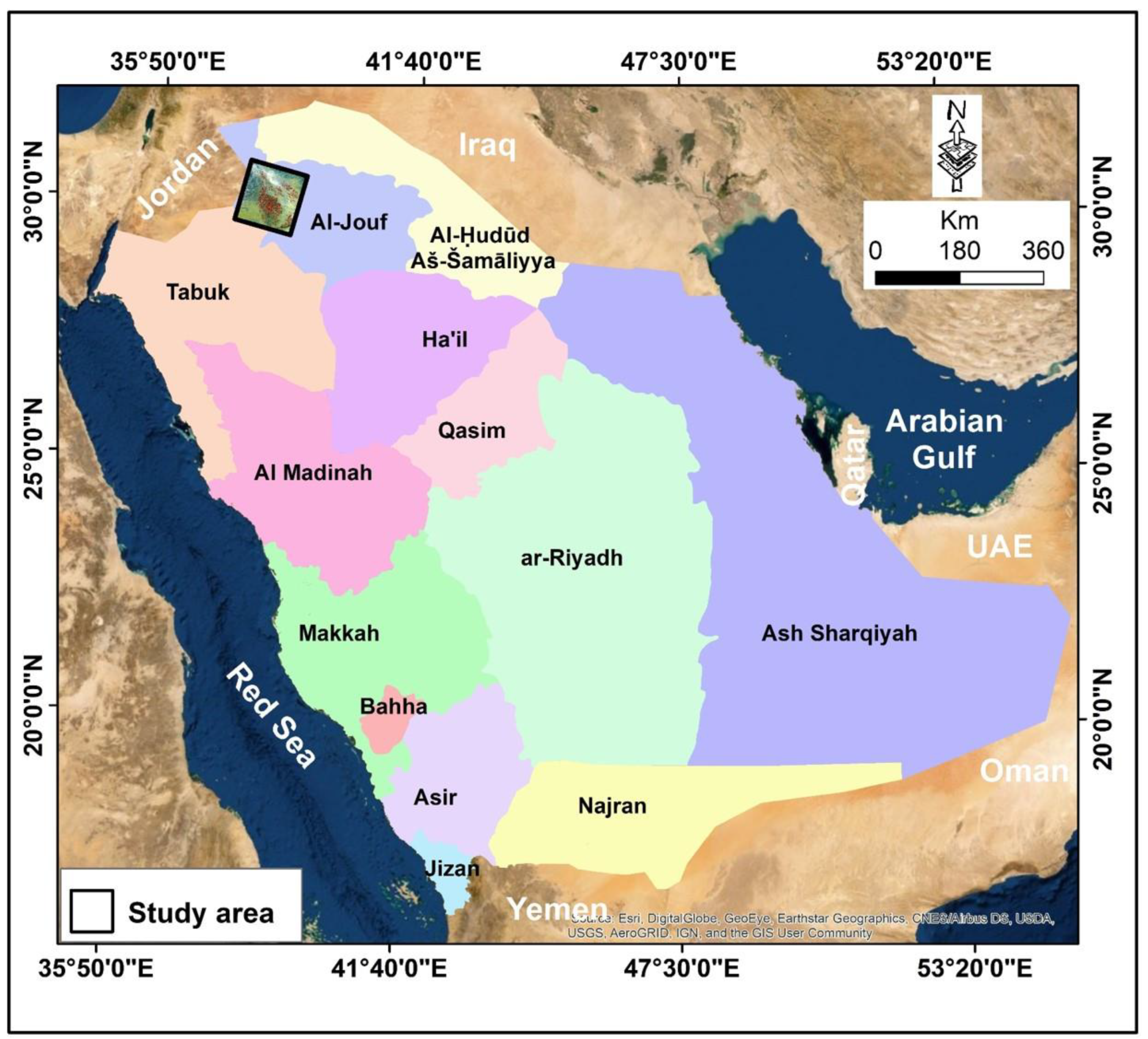
2. Study Area and Its Characteristics

The Al-Jouf agriculture area is located in the Al-Jouf region in the northern portion of the Kingdom of Saudi Arabia (KSA), occupying a vast stretch along the Wadi as Sirhan (Figure 1). It lies between latitudes 29°30′19″ and 30°56′2.0″ N and between longitudes 37°50′57″ and 39°02′13″ E. The study area is located mostly on the Southwestern fringe and along the Wadi as Sirhan. The agriculture activities in the area essentially depend on the groundwater aquifer (fossil water).

Al-Jouf region is characterized by hot desert climatic conditions, with limited precipitation and high temperatures [55]. The average yearly temperature in Al-Jouf is about 22.2 °C and the average rainfall is 59 mm.

Geologically, the study area is distinguished by different lithological units. The Sirhan Formation, dating from the Miocene–Pliocene Epochs, consists of friable calcareous sandstone, limestone, and shale beds that contain minor chert and clay beds [56]. The Harrat al Harrah rocks, the Upper Tertiary and Quaternary rocks, are composed of flood basalts that overlie the Tertiary sedimentary rocks (Sirhan Formation) [57]. The Quaternary deposits include calcareous and gypsiferous duricrusts, gravel, eolian sand, alluvium, and sabkha deposits. These deposits are very hard to map separately because they overlap each other and have broad and vague boundaries [58,59]. The area is dominated mainly by unconsolidated gravel deposits, eolian sand, and alluvium (silt, sand, and gravel). The calcareous duricrust is massive, consolidated, hard, and has a rough weathering rubbly surface that resembles massive limestone. The eolian sediments commonly occur as sand sheets or dunes above the alluvial materials. These dunes are a combination of barchanoid ridge-type and linear (sief) dunes trending in an east to southeast direction as the result of northwesterly and southwesterly wind directions. Alluvial silt, sand, and gravel form extensive deposits in the Wadi as Sirhan and the smaller basins. These deposits are mostly interlayered sheets and lenticular masses of poorly sorted gravels and gravelly sands, moderately sorted sands, and clayey silts. The prominent elongated sabkhas are located along the northeast trending axis of the Wadi as Sirhan and are composed of silt and clay layers interbedded with gypsum and calcite.

3. Data and Methods

A multi-temporal data of Landsat Thematic Mapper (TM), an Enhanced Thematic Mapper Plus (ETM+), and an Operational Land Imager (OLI) were used in this study (

Table 1. Main characteristics of the remote sensing data applied in this study.

Factor	Landsat TM	Landsat ETM+	Landsat OLI
Date launched	March 1984	April 1999	February 2013
Orbit platform	Satellite	Satellite	Satellite
Life time	Minimum 5 years	Minimum 5 years	Minimum 5 years
Organization	NASA	NASA	NASA
Scene size	170 × 185 km	170 × 185 km	170 × 185 km
Altitude	919 km	919 km	705 km
Class	Optical	Optical	Optical
Spectral region and spatial resolution	VNIR 1, 2, 3, 4 (30 m) SWIR 5, 7 (30 m) TIR 6 (120 m)	VNIR 1, 2, 3, 4, 5 (30 m) SWIR 5, 7 (30 m) TIR 6 (60 m) Pan 8 (15 m)	VNIR 1, 2, 3, 4, 5 (30 m) SWIR 6, 7 (30 m) TIR 10, 11 (100 m) Cirrus 9 (30 m) Pan 8 (15 m)
Band wavelengths (µm)	○ B1: 0.45–0.52 µm ○ B2: 0.52–0.60 µm ○ B3: 0.63–0.69 µm ○ B4: 0.76–0.90 µm ○ B5: 1.55–1.75 µm ○ B6: 10.40–12.50 µm ○ B7: 2.08–2.35 µm	○ B1: 0.45–0.52 µm ○ B2: 0.52–0.60 µm ○ B3: 0.63–0.69 µm ○ B4: 0.76–0.90 µm ○ B5: 1.55–1.75 µm ○ B6: 10.40–12.50 µm ○ B7: 2.08–2.35 µm ○ B8: 0.52–0.90 µm	○ B1: 0.43–0.45 µm ○ B2: 0.45–0.51 µm ○ B3: 0.53–0.59 µm ○ B4: 0.64–0.67 µm ○ B5: 0.85–0.88 µm ○ B6: 1.57–1.65 µm ○ B7: 2.11–2.29 µm ○ B8: 0.50–0.68 µm ○ B9: 1.36–1.38 µm ○ B10: 10.6–11.19 µm ○ B11: 11.5–12.51 µm
Identification and dates of data used in this study	○ P/R/172/39 ○ 20 April 1988 ○ 28 April 1988 ○ 1 September 1990 ○ 18 February 1993 ○ 13 May 1998 ○ 29 September 2003 ○ 13 March 2006 ○ 19 April 2008	○ P/R/172/39 ○ 12 September 2000 ○ 27 March 2011	○ P/R/171/39 ○ 9 May 2015 ○ 19 April 2016 ○ 2 August 2017

Note: NASA = U.S. National Aeronautics and Space Agency; ETM+ = Enhanced Thematic Mapper Plus; OLI = Operational Land Imager; VNIR = very near infrared; SWIR = shortwave infrared; TIR = thermal infrared; P/R = path/raw; Pan = panchromatic; B = band.

). These data have 30 m special resolution and cover a time span from April 1987 to August 2007. Bands 4, 3, and 1 of the Landsat TM and ETM+ data and bands 5, 4, and 1 of the Landsat OLI were used to extract the areal extent of the agriculture areas of the Al-Jouf region and to create a time series for the evolution of agriculture activities between 1987 and 2017. Different techniques were applied to extract the agriculture areas, including the NDVI, which was used to predict all changes that occurred in the agriculture activities using the ENVI 5.0 program. NDVI was derived from the satellite images. It was calculated from the red band and the NIR band for each sensor type, according to Equation (1) [60].

$$NDVI=\frac{NIR-Red}{NIR+Red}$$

(1)

This appeared very clearly in the 4–3–1 bands (band 4 is the NIR band; band 3 is the red band; and band 1 is the blue band) of Landsat TM and ETM+ images and in the 5–4–1 bands (band 5 is the NIR band; band 4 is the red band; and band 1 is the coastal aerosol band) of Landsat OLI, wherein the agriculture areas of the Al-Jouf region (red) can be distinguished from the surrounding geologic units of the region (Figure 2). A high NDVI value indicates that the density of vegetation is high, and a lower NDVI value means lower density or no vegetation. The NDVI images were exported into ArcGIS 10.2, then the agriculture areas were extracted from the NDVI images using a threshold value of 0.35. The results were validated by applying visual comparisons with high-resolution Google Earth images. However, according to the limitation in the application of the NDVI technique [41,42], the maximum likelihood technique (supervised classification techniques) was used [45,46] in ArcGIS 10.2 to extract all agriculture areas. The results of NDVI and supervised classification were compared with each other and with the original image for each period. Visual inspection was conducted to ensure that all of the agriculture areas were taken into account. Comparison of these techniques with the original images for each time period show that ~1% to 7% of the agriculture areas were not identified. So, hand digitization was applied on the ArcGIS screen to produce more accurate agriculture maps. The final results were subsequently used to calculate the area of the total agriculture activities for each image. The change in the agriculture areas was presented as a function of time. A relationship between the agriculture activities and the extraction of groundwater from the aquifer was established due to the documented data concerning the drawdown effect. To calculate the total volume of the groundwater extraction for each time interval of agriculture activities four equations were applied (Equations (2)–(5)).

First: Equation (2) was used to calculate the number of agriculture circles for each change rate:

$$N=\frac{\Delta \mathrm{A}}{0.503}$$

(2)

where N is the number of agriculture circles for each rate value; $\Delta \mathrm{A}$ is the rate of agriculture changes per year; and the average area of each agriculture circle was assumed to be 0.503 km².

Second: The total number of agriculture circles (Nt) during the time interval (Tn) can be calculated using Equation (3):

$$Nt=N\left(first year\right)+N\ast 2 \left(second year\right)+\cdots N\ast n \left(last year\right)$$

(3)

where n = 1, 2, 3, ……n.

For example, Nt for the time interval from 1988 to 1990 (time interval (Y) of 2.5 years with the number of agriculture circles (N = 121.95)) can be calculated using Equation (3): Nt = 121.95 + 121.95 × 2 + 121.95 × 3 × 0.5 = 548.79.

This methodology was applied for all the time intervals to estimate the number of agriculture circles at each time interval.

Third: As we assumed that each agriculture circle would be irrigated by one water well, the volume of water (V) (million cubic meters (MCM)) that was extracted from the aquifer for each time interval could then be estimated using Equation (4):

$$V=\frac{Nt\ast 16\ast 200\ast 192}{1000000}$$

(4)

where V is the volume of extracted water from the aquifer (MCM); Nt is the total number of agriculture circles planted during the time interval (Y); 16, 200, and 192 are the assumptions for number of hours per day, number of days per year, and well-pumping rate per hour (cubic meter per hour).

Fourth: The total volume of water extracted from the aquifer (Vt) for the total number of agriculture years (Yt) at each time interval up until August 2017 was calculated using Equation (5).

$$Vt=V\ast Yt$$

(5)

where (Yt) is the total number of agriculture years from each interval until the end of the recorded time period (August 2017).

In addition, fieldwork was conducted to map different types of sinkholes in the study area.

4. Results

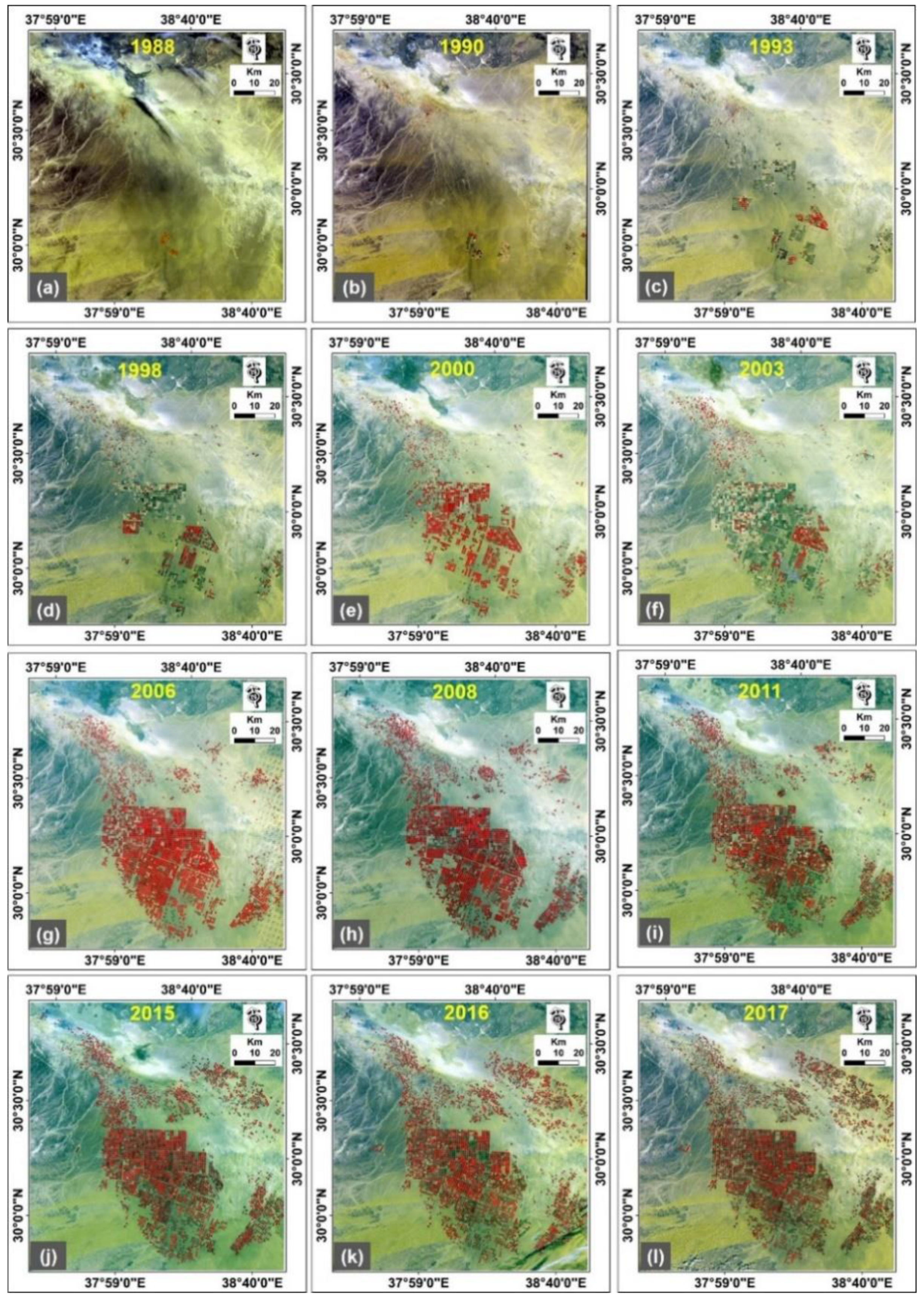
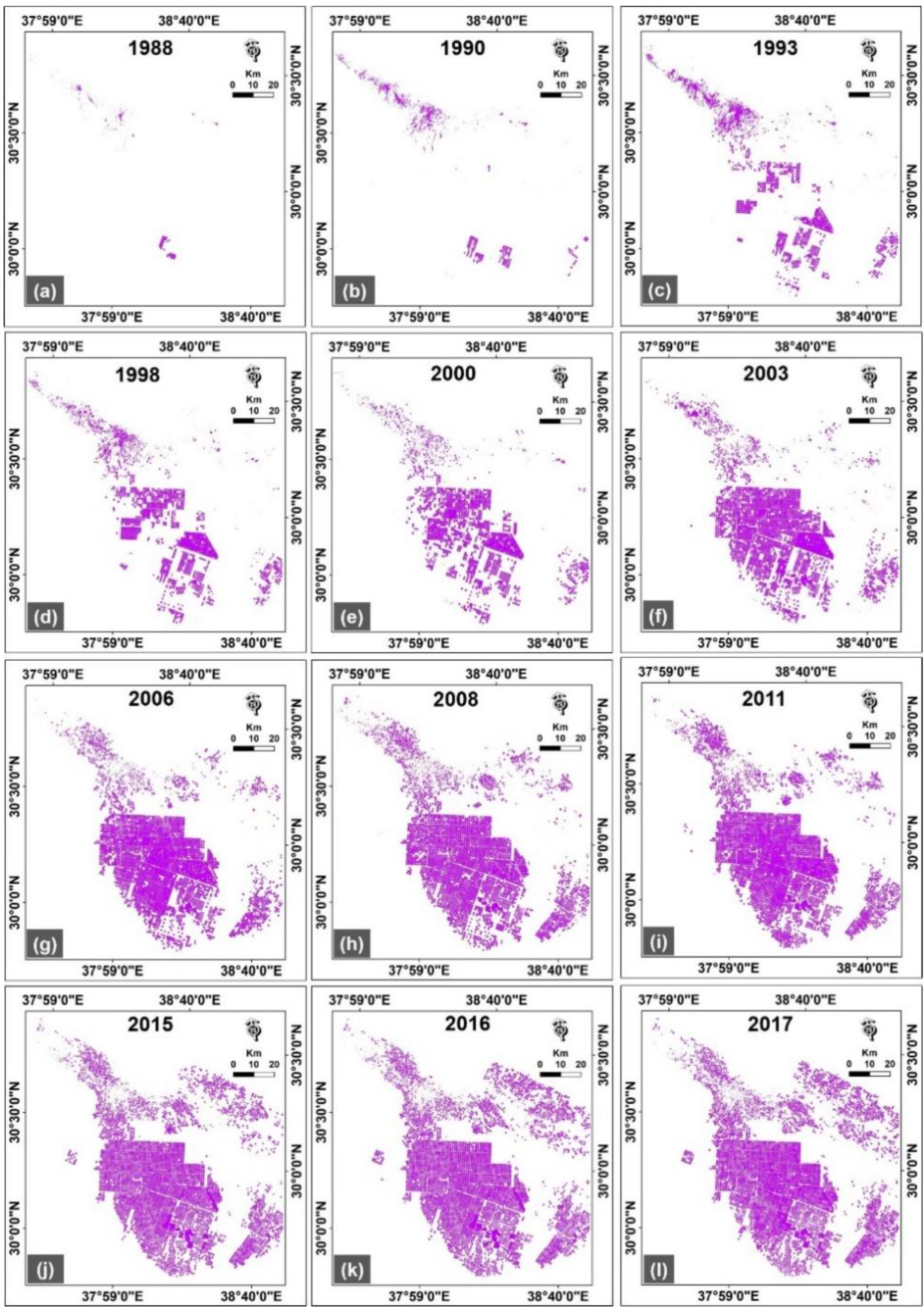
4.1. Temporal Evolution of Agriculture Activities Using RS and GIS

Agriculture activity development will have an impact on the environment. The current study area has been subjected to substantial agricultural changes over the last few decades. To detect these agricultural changes, the temporal evolution of the agriculture activities of the Al-Jouf region was mapped out over 12 periods from 1987 to 2017 (Figure 2 and Figure 3 and

Table 2. Changes in agriculture areas between 1987 and 2017.

A	B	C	D (km2)	E (Year)	F (km2)	G (Year)	H (km2/Year)	I (km2/Year)
1	S1-1	28/4/1988	37.9	From 20 April 1987 to 28 April 1988	37.9	1	37.9	37.9
2	S2-1	01/9/1990	191.3	From 28 April 1988 to 01 September 1990	153.4	2.5	61.3	132.4
	S2-2	18/2/1993	700.0	From 01 September 1990 to 18 February 1993	508.8	2.5	203.5
3	S3-1	13/5/1998	935.5	From 18 February 1993 to 13 May 1998	235.5	5.3	44.4	44.4
4	S4-1	12/9/2000	1119.5	From 13 May 1998 to 12 September 2000	184.0	2.3	79.9	159.1
	S4-2	29/9/2003	1807.4	From 12 September 2000 to 29 September 2003	687.9	3	229.3
	S4-3	13/3/2006	2176.2	From 29 September 2003 to 13 March 2006	368.8	2.5	147.5
5	S5-1	19/4/2008	2266.2	From 13 March 2006 to 19 April 2008	90.0	2.1	42.9	30.5
	S5-2	27/3/2011	2410.5	From 19 April 2008 to 27 March 2011	144.3	3	48.1
	S5-3	9/5/2015	2459.6	From 27 March 2011 to 9 May 2015	49.1	4.2	11.7
6	S6-1	19/4/2016	2651.6	From 9 May 2015 to 19 April 2016	191.9	1	191.9	119.5
	S6-2	02/8/2017	2734.6	From 19 April 2016 to 02 August 2017	83.0	1.3	63.9

A= sub-stage number; B = steps; C = image date; D = total agriculture area (km²); E = span interval (Year); F = changes of each interval (km²); G = number of years in each interval (Year); H = rate of changes (km²/year); I= overall change rate (km²/year).

).

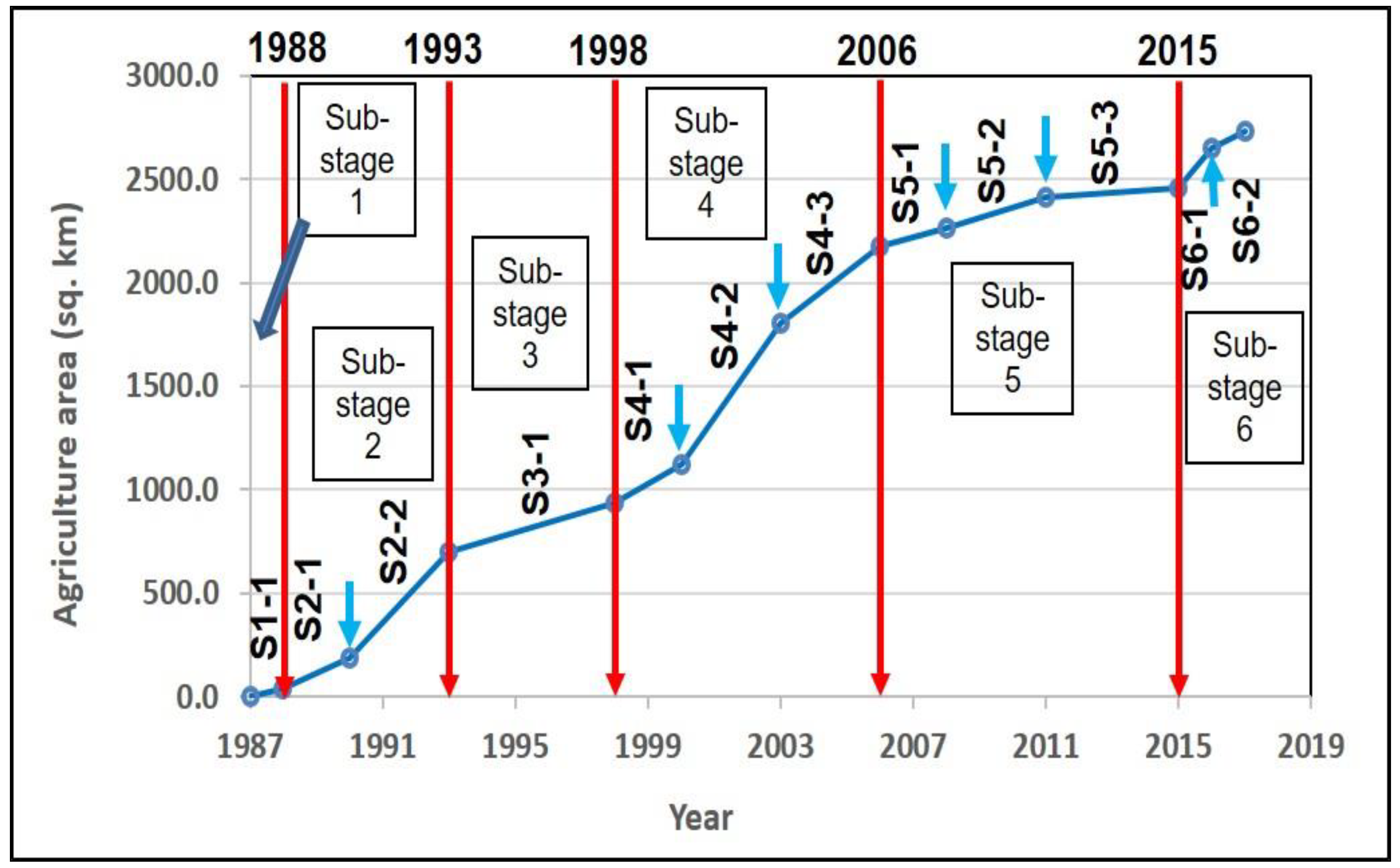
4.2. Stages of Agriculture Sprawl of the Al-Jouf Region

Results indicated that two main stages characterize the agriculture activities in the study area: 1) A low rising stage, which includes three sub-stages (1, 3, and 5) (Table 2 and Figure 4). This stage is marked by less development of the agriculture activities in the area as the agriculture activities during this stage started to decrease rapidly. 2) A high rise stage, which includes three sub-stages (2, 4, and 6) (Table 2 and Figure 4). This stage is distinguished by a rapid development rate of agriculture activities in the area.

The overall change for each sub-stage was calculated as ~37.9, ~132.4, ~44.4, ~159.1, ~30.0, and ~119.5 km²/year for sub-stages 1, 2, 3, 4, 5, and 6, respectively (Table 2). In the following parts, these sub-stages will be discussed chronologically, from sub-stage 1 (old) to sub-stage 6 (recent).

Sub-stage (1) has an overall change of 37.9 km² per year. It is characterized by one step (S1-1), which started on 20 April 1987 and ended on 28 April 1988, and covered an area of ~37.9 km² for the span of one year (Table 2 and Figure 4).

Sub-stage (2) has an overall average agriculture change of 132.4 km² per year. It is characterized by two steps S2-1 and S2-2 (Table 2 and Figure 4). Step S2-1 coves an area of ~153.4 km² for a span of 2.5 years, with a change rate of ~61.3 km² per year. In step S2-2, the sprawl of agriculture activities occurred toward the northwest and east directions resulting in the agriculture development covering an area of ~508.8 km² for a span of 2.5 years with a rate of ~203.5 km² per year.

Sub-stage (3) has an overall change of 44.4 km² per year. It is characterized by one step (S3-1), covering an area of ~235.5 km² for a span of 5.3 years, with a change rate of ~44.4 km² per year (Table 2 and Figure 4).

Sub-stage (4) has an overall change of 159.1 km² per year, and consists of three steps (S4-1, S4-2, and S4-3) (Table 2 and Figure 4). In this sub-stage, the agriculture activities started sprawling in the northwest and east directions. Step (S4-1) covers an area of ~184 km², for a span of 2.3 years, with a change rate of ~79.9 km² per year. Step (S4-2) of this sub-stage represents the main abrupt change in the agriculture activities, at which point Saudi Arabia encouraged local people and private sectors to develop agriculture activities. The agriculture area in this step reaches an area of ~687.9 km² for a span of three years with a change rate of ~229.3 km² per year. In step (S4-3) the agriculture activities cover an area of ~368.8 km² for a span of 2.5 years, with a change rate of ~147.5 km² per year.

Sub-stage (5) has an overall change of 30 km² per year. The agriculture activities in this sub-stage are characterized by three steps (S5-1, S5-2, and S5-3) (Figure 4 and Table 2). Step (S5-1) occupied an area of ~90.0 km² for a span of 2.1 years with a change rate of ~42.9 km² per year. Step (S5-2) covers an area of ~144.3 km² for a span of three years with a change rate of ~48.1 km² per year. Step (S5-3) has an area of ~49.1 km² for a span of 4.2 years with an agriculture change rate of ~11.7 km² per year.

Sub-stage (6) has an overall change of 119.5 km² per year. The agriculture activities in this sub-stage followed two steps (S6-1 and S6-2) (Table 2 and Figure 4). In step (S6-1), the rate of the agriculture activities dramatically increased, covering an area of ~191.9 km² for a span of 1 year, with a change rate of ~191.9 km² per year. In step (S6-2), the agriculture development covers an area of ~83 km² for a span of 1.3 years, with a change rate of ~63.9 km² per year.

4.3. Environmental Impact of Uncontrolled Agriculture Activities

4.3.1. Groundwater Extraction Quantity and Drawdown

According to the analysis of the agriculture sprawl in the Al-Jouf region, it was found that the agricultural land increased from ~37.9 to 2734.6 km² during the period from 1988 to 2017. The agriculture areas solely depended on irrigation using the groundwater aquifer (fossil groundwater). Water extracted from the aquifer increased dramatically in three sub-stages including sub-stage (2) from 1988 to 1993 (a span of 5 years, with an overall agriculture change rate of ~132.4), sub-stage (4) from 1998 to 2006 (a span of 7.8 years, with an overall agriculture change rate of ~159.1), and sub-stage (6) from 2016 to 2017 (span of 2.3 years with an overall agriculture change rate of ~119.5). The groundwater level drop reached 150 meters by August 2017 according to data acquired from the farmers in the area. The average groundwater quantity extracted from the aquifer during the period from 1987 to 2017 was estimated according to the agriculture areas at each time interval. The current study is based on the data collected by the authors of [61,62]. They indicated that the groundwater extraction reached 2000 million cubic meter per year (MCM/year) in 2004 which used for an agriculture area covering ~1640 km². According to that, some assumptions were utilized in the current study due to a lack of detailed data about the number of wells, pumping capacity, the number of working hours for each well per day, and the number of operating days per year. These assumptions were determined, according to various field visits and the information acquired from the farmers in the area, and the following assumptions were considered: (1) the number of wells was estimated according to the total agriculture area divided by the area of the average agriculture circle (the average agriculture circle diameter was ~800 m with an area of ~0.503 km², and it included one water well for irrigation); (2) the rate of operation for each well was assumed to be 16 h per day, working approximately 200 days each year (according to the information acquired from the farmers, where more than 165 days were excluded due to the time between planting crops, harvesting, and winter time, when some days were taken off due to low evaporation values).

Accordingly, the average rate of each water well was calculated to be ~192 cubic meter per hour. The total amount of groundwater extracted from the subsurface aquifer was calculated according to the application of the above assumptions using Equations (2)–(5).

Our findings revealed that the total volume of water extracted from the subsurface aquifer reached ~119,118.5 MCM in August 2017 (

Table 3. Calculation of water consumptions due to agriculture activities from 1987 to 2017.

Period (Interval)	ΔA (km2/year)	N	Y (Year)	Nt	V (MCM)	Yt (Year)	Vt (MCM)
From 24 April 1987 to 28 April 1988	37.9	75.40	1	75.40	46.33	30.7	1422.19
From 28 April 1988 to 01 September 1990	61.3	121.95	2.5	548.79	337.17	29.7	10,014.07
From 01 September 1990 to 18 February 1993	203.5	404.85	2.5	1821.83	1119.33	27.2	30,445.77
From 18 February 1993 to 13 May 1998	44.4	88.33	5.3	1483.96	911.75	24.7	22,520.10
From 13 May 1998 to 12 September 2000	79.9	158.96	2.3	619.93	380.88	19.4	7389.15
From 12 September 2000 to 29 September 2003	229.3	456.18	3	2737.07	1681.65	17.1	28,756.27
From 29 September 2003 to 13 March 2006	147.5	293.44	2.5	1320.49	811.31	14.1	11,439.44
From 13 March 2006 to 19 April 2008	42.9	85.35	2.1	281.64	173.04	11.6	2007.29
From 19 April 2008 to 27 March 2011	48.1	95.69	3	574.15	352.76	9.5	3351.21
From 27 March 2011 to 9 May 2015	11.7	23.28	4.2	256.04	157.31	6.5	1022.52
From 9 May 2015 to 19 April 2016	191.9	381.77	1	381.77	234.56	2.3	539.49
From 19 April 2016 to 02 August 2017	83	165.12	1.3	264.20	162.32	1.3	211.02
The total amount of water consumed from the aquifer (MCM)							119,118.5

ΔA = rate of change of agriculture area; N = number of used circles per year for each rate; Y = number of years for each span interval; N_t = total number of used circles during the time span; V = volume of water consumed, million cubic meters (MCM); Yt = total number of agriculture years; Vt = total volume of water consumed up to August 2017.

). This value represents a tremendous amount of water pumped out of the subsurface aquifer.

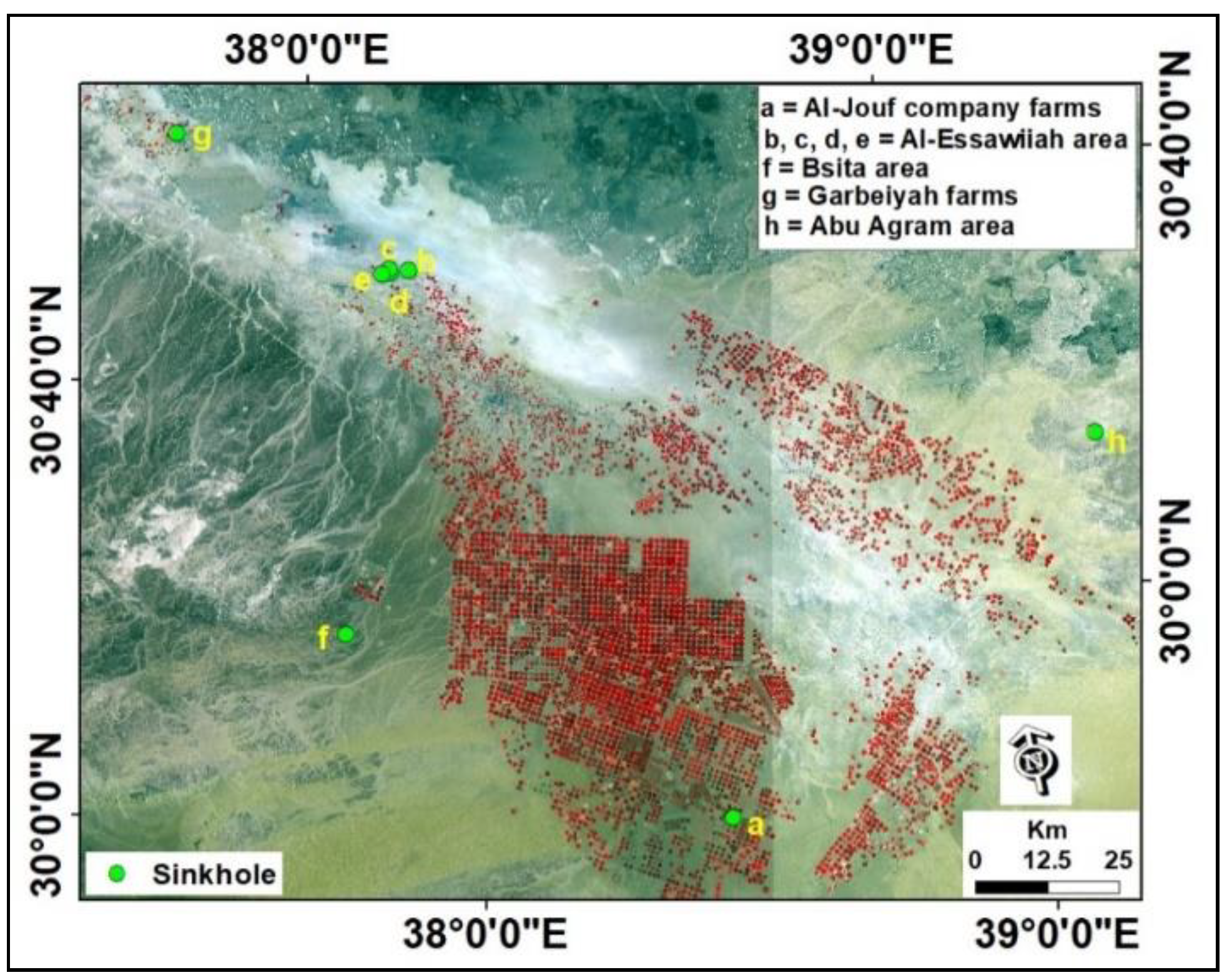
4.3.2. Human-Induced Sinkholes

Sinkholes are considered to be the most frequently recognized phenomena causing geological and environmental hazards in the KSA [11,12]. They are formed in carbonate and evaporite rocks. Many sinkholes have been encountered in the Al-Jouf region (

Table 4. The main characteristics of different sinkholes in the Al-Jouf region.

S. No.	Area Name	Lat. (North)	Long. (East)	Dimensions (Meters)	Mechanism Type	Year of Occurrence
a	Al-Jouf farms	29°46′44″	38°27′37″	Di = 40 m, De = 15 m	Cover-collapse	~2013
b	Essawiah area	30°43′31″	38°06′01″	Di = 27 m, De = 23 m	Caprock-collapse	~2004
c	Essawiah area	30°43′39″	38°04′05″	Di = 30 m, De = 2.5 m	Cover-collapse	~2012
d	Essawiah area	30°44′06″	38°04′04″	Di = 45 m, De = 0.5 m	New-formed	~2012
e	Essawiah area	30°43′43″	38°03′14″	Di = 30 m, De = 1 m	New-formed	~2012
f	Bsita area	30°11′17″	37°51′02″	L= 100 m, W = 60 m, De = 30 m	Sagging-collapse	Before 1984
g	Al Nasfah area	30°0′47″	37°44′43″	Di = 25 m, De = 25 m	Caprock-collapse	2018
h	Abu Agram area	30°14′39″	39°14′58″	Di = 3 m, De = 20 m	Dallin type	~2010

S. No. = sinkhole number; Lat. = latitude; Long. = longitude; Di = diameter; De = depth; L = length; W = width; ~ = around.

). These subsidence processes, including sinkhole formation, can be triggered or accelerated by various human activities such as severe groundwater extraction from the subsurface aquifer system [63,64,65]. This aquifer system holds nonrenewable water (fossil water). Most of the Al-Jouf sinkholes have appeared in and are surrounded by agriculture activities (Figure 5). Many authors have indicated that the main karst limestone rock in the Al-Jouf region is Sirhan Formation, which is located in the northern portion of the Arabian Platform [11]. These sinkholes are associated with different mechanisms [11,12]. Some of them are extremely dangerous and occur suddenly with no warning. However, others show some clear evidence (tension cracks and small subsidence features) before occurring. Studies carried out by Youssef et al. [11] indicated that Al-Jouf sinkholes are related to the subsidence mechanism. The term subsidence sinkhole applies to both carbonate and evaporite karst territories. It was classified by Gutiérrez et al. [64,66,67]. This classification uses two titles: the first description applies to the materials influenced by subsidence (cover, bedrock, and caprock), and the second term indicates the subsidence mechanism (collapse, suffosion, and sagging). The term "cover" demonstrates the unconsolidated deposits, bedrock to karst rocks, and caprock to non-karst rocks. Collapse is the brittle deformation of soils or rock materials, either by brecciation or the evolution of distinct failure planes. Suffosion is the downward movement of the unconsolidated top deposits through the conduits and its gradual settling, and sagging is the descending bending of the ductile sediments. Complex sinkholes, including more than one material type and numerous subsidence mechanisms, are illustrated using the combinations of the proposed terms, with the predominant material and process followed by the secondary ones.

4.4. The Future Trend of Agriculture Activities and Groundwater Drawdown

If the agriculture activity rate becomes constant, as the rate between 2016 and 2017 (83 km²/year) did, we can easily calculate the amount of water that could be extracted from the aquifer for the next 10 years as follows:

• The amount of water extracted in 2017 can be calculated using the following equation, taking into account the aforementioned assumptions. Total area in 2017 is ~2734 km²; the number of agriculture circles is 5446, which is equal to the number of water wells; so the quantity of extracted groundwater from the subsurface aquifer is ~5440.3 × 16 × 200 × 192 = ~3342.5 MCM. This amount after 10 years is equal to ~33,425.0 MCM.
• The amount of water for the change rate of 83 km²/year for 10 years can be calculated according to the previous equation to be ~5579.8 MCM.
• The predicted total amount extracted from the aquifer will thus be 33,425.0 + 5579.8 = ~39005.1 MCM.
• The amount of extracted water for the future 10 years will be about 32.7% of the amount of water extracted in the last 31 years (~119,118.5 MCM). This amount of extracted water will contribute to more groundwater depletion by the end of the next 10 years. The increase in groundwater depletion will trigger more sinkholes in the area.
• The current study can be an outstanding base for future groundwater modeling study to understand the value and trend of the groundwater depletion. This can be done by studying the monitoring wells in the study area and its surroundings, which are operated by the Water Resources Development Department in the Ministry of Environment, Water and Agriculture.

5. Conclusions

In the current study, an integrated approach utterly relying on readily available remote sensing data sets was used to map the agriculture sprawl in the Al-Jouf area. The relationship between the agriculture activities and the total volume of groundwater extraction was discussed. Finally, environmental consequences of these agriculture activities (the depletion of the aquifer and occurrence of sinkholes) were explained.

Since 1987, the Al-Jouf region has expanded its agriculture activities dramatically and it is expected that more areas will undergo agriculture expansion in the region in future years, leading to excessive and increasing exploitation of fossil aquifers, which will subsequently cause aquifer depletion and increase the number of sinkholes. This study illustrates that the land deformation-features (sinkholes) are related to water extraction due to agricultural sprawl in the northern part of Saudi Arabia (Al-Jouf region). Pumping groundwater from limestone aquifers in the study area, the Sirhan Formation, was associated with a drop in water levels in the area. The substantial drop of the groundwater table leads to removal of the fine sediments and water from the subsurface preexisting cavities, leaving them empty. This could result in the loss of buoyant support causing a “non-equilibrium” in the area, causing a collapse of the above sediments and rocks due to gravity (weight) or other external effects (irrigation water, rainfall, flood water). Some of these cavities may remain hidden under the cover of materials, but over time they will collapse (some have appeared recently in 2018).

Managing the agriculture expansion in the area plays a critical role in ensuring the future of the local groundwater aquifer system. There is thus an urgent need for a groundwater management system to alleviate the impact that accelerated agriculture development will have on natural resources (groundwater aquifer) in the Al-Jouf region. In addition, environmental problems (sinkholes) are associated with the drop of the water table in the area. Our procedures could potentially be used to predict the future trend of agriculture activities, groundwater depletion and land deformation in the area. Finally, this study could provide a replicable result for decision-makers to ensure optimum utilization of fossil aquifers and to minimize the associated environmental impacts.

References

1. International Food Policy Research Institute (IFPRI). Global Food Policy Report; IFPRI: Washington, DC, USA, 2017; Available online: http://www.Ifpri.Org/publication/2017-global-food-policy-report (accessed on 12 October 2017).
2. Vibhute, A.D.; Gawali, B.W. Analysis and Modeling of Agricultural Land use using Remote Sensing and Geographic Information System: A Review. Int. J. Eng. Res. Appl. 2012, 3, 81–91. [Google Scholar]
3. Şatir, O. Mapping the Land-Use Suitability for Urban Sprawl Using Remote Sensing and GIS under Different Scenarios. In Sustainable Urbanization; Ergen, M., Ed.; InTech: Horwich, UK, 2016; pp. 205–226. [Google Scholar]
4. Yu, J.; Wu, J. The Sustainability of Agricultural Development in China: The Agriculture—Environment Nexus. Sustainability 2018, 10, 1776. [Google Scholar] [CrossRef]
5. Othman, A.; Sultan, M.; Becker, R.; Alsefry, S.; Alharbi, T.; Gebremichael, E.; Alharbi, H.; Abdelmohsen, K. Use of Geophysical and Remote Sensing Data for Assessment of Aquifer Depletion and Related Land Deformation. Surv. Geophys. 2018, 39, 543–566. [Google Scholar] [CrossRef] [PubMed] [Green Version]
6. Konikow, L.F.; Kendy, E. Groundwater depletion: A global problem. Hydrogeol. J. 2005, 13, 317–320. [Google Scholar] [CrossRef]
7. Khair, S.M.; Culas, R.J.; Hafeez, M. The causes of groundwater decline in upland Balochistan region of Pakistan: Implication for water management policies. In Proceedings of the Australian Conference of Economists (ACE10), Sydney, Australia, 27–29 September 2010. [Google Scholar]
8. Dixon, M. Plastics and Agriculture in the Desert Frontier. Comp. Stud. S. A Afr. Middle E 2017, 37, 86–102. [Google Scholar] [CrossRef] [Green Version]
9. Zhou, Y.; Dong, D.; Liu, J.; Li, W. Upgrading a regional groundwater level monitoring network for Beijing Plain, China. Geosci. Front. 2013, 4, 127–138. [Google Scholar] [CrossRef] [Green Version]
10. Nassif, M. Groundwater Governance in the Central Bekaa, Lebanon; IWMI Project Report No. 10; USAID: Washington, DC, USA, 2016; p. 129. [Google Scholar]
11. Youssef, A.M.; Al-Harbi, H.M.; Zabramwi, Y.A.; El-Haddad, B.A. Human-Induced Geo-Hazards in the Kingdom of Saudi Arabia: Distribution, Investigation, Causes and Impacts. In Geohazards Caused by Human Activity; Farid, A., Ed.; InTech: Horwich, UK, 2016; pp. 37–61. [Google Scholar]
12. Youssef, A.M.; Al-Harbi, H.M.; Gutiérrez, F.; Zabramwi, Y.A.; Bulkhi, A.B.; Zahrani, S.A.; Bahamil, A.M.; Zahrani, A.J.; Otaibi, Z.A.; El-Haddad, B.A. Natural and human-induced sinkhole hazards in Saudi Arabia: Distribution, investigation, causes, and impacts. Hydrogeol. J. 2016, 24, 625–644. [Google Scholar] [CrossRef]
13. Ramachandra, T.V.; Kumar, U. Geographic Resources Decision Support System for land use/land cover dynamics analysis. In Proceedings of the FOSS/GRASS Users Conference, Bangkok, Thailand, 12–14 September 2004; pp. 12–14. [Google Scholar]
14. Abdelsalam, M.G.; Youssef, A.M.; Arafat, S.M.; Alfarhan, M. The Rise and Demise of the New Lakes of Sahara. Geosphere 2008, 4, 375–386. [Google Scholar] [CrossRef]
15. Im, J.; Jensen, J.; Tullis, J. Object-based change detection using correlation image analysis and image segmentation. Int. J. Remote Sens. 2008, 29, 399–423. [Google Scholar] [CrossRef]
16. Şatir, O.; Berberoğlu, S. Land use/cover classification techniques using optical remotely sensed data in landscape planning. In Landscape Planning. Rijeka; Özyavuz, M., Ed.; InTech: Horwich, UK, 2012; pp. 21–54. [Google Scholar]
17. Raziq, A.; Xu, A.; Li, Y.; Zhao, Q. Monitoring of land use/land cover changes and urban sprawl in Peshawar City in Khyber Pakhtunkhwa: An application of geo-information techniques using of multi-temporal satellite data. J. Remote Sens. 2016, 5, 174. [Google Scholar] [CrossRef]
18. Berberoglu, S.; Satir, O.; Atkinson, P.M. Mapping percentage tree cover from Envisat MERIS data using linear and non-linear techniques. Int. J. Remote Sens. 2009, 30, 4747–4766. [Google Scholar] [CrossRef]
19. Donmez, C.; Berberoglu, S.; Curran, P. Modelling the current and future spatial distribution of NPP in a Mediterranean watershed. Int. J. Appl. Earth Obs. Geoinf. 2011, 13, 336–345. [Google Scholar] [CrossRef]
20. Akin, A.; Sunar, F.; Berberoğlu, S. Urban change analysis and future growth of Istanbul. Environ. Monit. Assess. 2015, 187, 506. [Google Scholar] [CrossRef] [PubMed]
21. Alqurashi, A.; Kumar, L.; Sinha, P. Urban land cover change modeling using time-series satellite images: A case study of urban growth in five cities of Saudi Arabia. Remote Sens. 2016, 8, 838. [Google Scholar] [CrossRef]
22. Liu, F.; Zhang, Z.; Wang, X. Forms of urban expansion of Chinese municipalities and provincial capitals, 1970s–2013. Remote Sens. 2016, 8, 930. [Google Scholar] [CrossRef]
23. Cao, H.; Liu, J.; Fu, C.; Zhang, W.; Wang, G.; Yang, G.; Luo, L. Urban expansion and its impact on the land use pattern in xishuangbanna since the reform and opening up of China. Remote Sens. 2017, 9, 137. [Google Scholar] [CrossRef]
24. Gumma, M.K.; Mohammad, I.; Nedumaran, S.; Whitbread, A.; Lagerkvist, C.J. Urban Sprawl and Adverse Impacts on Agricultural Land: A Case Study on Hyderabad, India. Remote Sens. 2017, 9, 1136. [Google Scholar] [CrossRef]
25. Parece, T.E.; Campbell, J.B. Geospatial evaluation for urban agriculture land inventory: Roanoke, Virginia USA. Int. J. Appl. Geospat. Res. 2017, 8, 43–63. [Google Scholar] [CrossRef]
26. Ambast, S.K.; Keshari, A.K.; Gosain, A.K. Satellite Remote Sensing to support management of irrigation systems: Concepts and approaches. Irrig. Drain. 2002, 51, 25–39. [Google Scholar] [CrossRef]
27. Waldner, F.; Canto, G.S.; Defourny, P. Automated annual cropland mapping using knowledge-based temporal features. ISPRS J. Photogramm. Remote Sens. 2015, 110, 1–13. [Google Scholar] [CrossRef]
28. Kingra, P.K.; Majumder, D.; Singh, S.P. Application of Remote Sensing and GIS in agriculture and natural resource management under changing climatic conditions. Agric. Res. J. 2016, 53, 295–302. [Google Scholar] [CrossRef]
29. Wójtowicz, M.; Wójtowicz, A.; Piekarczyk, J. Application of Remote Sens. methods in agriculture. Commun. Biometry Crop Sci. 2016, 11, 31–50. [Google Scholar]
30. Sonobe, R.; Yamaya, Y.; Tani, H.; Wang, X.; Kobayashi, N.; Mochizuki, K. Assessing the suitability of data from Sentinel-1A and 2A for crop classification. GISci. Remote Sens. 2017, 54, 918–938. [Google Scholar] [CrossRef]
31. Xiong, J.; Thenkabail, P.S.; Gumma, M.K.; Teluguntla, P.; Poehnelt, J.; Congalton, R.G.; Yadav, K.; Thau, D. Automated cropland mapping of continental Africa using Google earth engine cloud computing. ISPRS J. Photogramm. Remote Sens. 2017, 126, 225–244. [Google Scholar] [CrossRef]
32. Belgiu, M.; Csillik, O. Remote Sensing of Environment Sentinel-2 cropland mapping using pixel-based and object-based time-weighted dynamic time warping analysis. Remote Sens. Environ. 2018, 204, 509–523. [Google Scholar] [CrossRef]
33. Pareeth, S.; Karimi, P.; Shafiei, M.; De Fraiture, C. Mapping agricultural landuse patterns from time series of Landsat 8 using random forest based hierarchial approach. Remote Sens. 2019, 11, 601. [Google Scholar] [CrossRef]
34. Shanmugapriya, P.; Rathika, S.; Ramesh, T.; Janaki, P. Applications of Remote Sensing in Agriculture—A Review. Int. J. Curr. Microbiol. Appl. Sci. 2019, 8, 2270–2283. [Google Scholar] [CrossRef]
35. Hamel, S.; Garel, M.; Festa-Bianchet, M.; Gaillard, J.M.; Côté, S.D. Spring Normalized Difference Vegetation Index (NDVI) predicts annual variation in timing of peak faecal crude protein in mountain ungulates. J. Appl. Ecol. 2009, 46, 582–589. [Google Scholar] [CrossRef]
36. Byomkesh, T.; Nakagoshi, N.; Dewan, A.M. Urbanization and green space dynamics in Greater Dhaka, Bangladesh. Landsc. Ecol. Eng. 2012, 8, 45–58. [Google Scholar] [CrossRef]
37. Dewan, A.M.; Yamaguchi, Y.; Ziaur Rahman, M. Dynamics of land use/cover changes and the analysis of landscape fragmentation in Dhaka Metropolitan Bangladesh. GeoJournal 2012, 77, 315–330. [Google Scholar] [CrossRef]
38. Gray, J.; Friedl, M.; Frolking, S.; Ramankutty, N.; Nelson, A.; Gumma, M. Mapping Asian cropping intensity with MODIS. IEEE J. Sel. Top. Appl. Earth Obs. Remote Sens. 2014, 7, 3373–3379. [Google Scholar] [CrossRef]
39. Xu, D.; Guo, X. Compare NDVI Extracted from Landsat 8 Imagery with that from Landsat 7 Imagery. Am. J. Remote Sens. 2014, 2, 10–14. [Google Scholar] [CrossRef]
40. Gumma, M.K.; Kajisa, K.; Mohammed, I.A.; Whitbread, A.M.; Nelson, A.; Rala, A.; Palanisami, K. Temporal change in land use by irrigation source in Tamil Nadu and management implications. Environ. Monit. Assess. 2015, 187, 1–17. [Google Scholar] [CrossRef] [PubMed]
41. Matsushita, B.; Yang, W.; Chen, J.; Onda, Y.; Qiu, G. Sensitivity of the Enhanced Vegetation Index (EVI) and Normalized Difference Vegetation Index (NDVI) to topographic effects: A case study in high-density cypress forest. Sensors 2007, 7, 2636–2651. [Google Scholar] [CrossRef] [PubMed]
42. Tittebrand, A.; Spank, U.; Bernhofer, C.H. Comparison of satellite and ground-based NDVI above different land-use types. Theor. Appl. Climatol. 2009, 98, 171–186. [Google Scholar] [CrossRef]
43. Joshi, P.K.K.; Roy, P.S.; Singh, S.; Agrawal, S.; Yadav, D. Vegetation cover mapping in India using multi-temporal IRS Wide Field Sensor (WiFS) data. Remote Sens. Environ. 2006, 103, 190–202. [Google Scholar] [CrossRef]
44. Potapov, P.; Hansen, M.C.; Stehman, S.V.; Loveland, T.R.; Pittman, K. Combining MODIS and Landsat imagery to estimate and map boreal forest cover loss. Remote Sens. Environ. 2008, 112, 3708–3719. [Google Scholar] [CrossRef]
45. McLachlan, G. Discriminant Analysis and Statistical Pattern Recognition; John Wiley & Son: New York, NY, USA, 1992. [Google Scholar]
46. Richards, J.A.; Jia, X. Remote Sensing Digital Image Analysis: An Introduction, 4th ed.; Springer: Secaucus, NJ, USA, 2006; p. 439. [Google Scholar] [CrossRef]
47. Ministry of Agriculture and Water (MOAW). Number and Area of Agricultural Holdings with Land by Source of Irrigation in the Kingdom. Ministry of Water and Agriculture; Saudi Arabia Online Data; 2017. Available online: http://www.mewa.gov.sa (accessed on 2 August 2019).
48. Ouda, O.K. Impacts of agricultural policy on irrigation water demand: A case study of Saudi Arabia. Int. J. Water Resour. Dev. 2014, 30, 282–292. [Google Scholar] [CrossRef]
49. Food and Agriculture Organization (FAO). Groundwater Management in Saudi Arabia; Draft Synthesis Report; FAO: Rome, Italy, 2009; p. 14. [Google Scholar]
50. Scheidt, J.; Lerche, I.; Paleologos, E. Environmental and economic risks from sinkholes in west-central Florida. Environ. Geosci. 2005, 12, 207–217. [Google Scholar] [CrossRef]
51. Sun, H.; Grandstaff, D.; Shagam, R. Land subsidence due to groundwater withdrawal: Potential damage of subsidence and sea level rise in southern New Jersey, USA. Environ. Geol. 1999, 37, 290–296. [Google Scholar] [CrossRef]
52. Zektser, S.; Loaiciga, H.A.; Wolf, J.T. Environmental impacts of groundwater overdraft: Selected case studies in the southwestern United States. Environ. Geol. 2005, 47, 396–404. [Google Scholar] [CrossRef]
53. Wolkersdorfer, C.; Thiem, G. Groundwater withdrawal and land subsidence in Northeastern Saxony (Germany). Mine Water Environ. Assoc. 2006, 18, 81–92. [Google Scholar] [CrossRef]
54. Xu, Y.S.; Shen, S.L.; Cai, Z.Y.; Zhou, G.Y. The state of land subsidence and prediction approaches due to groundwater withdrawal in China. Nat. Hazards 2008, 45, 123–135. [Google Scholar] [CrossRef]
55. Peel, M.C.; Finlayson, B.L.; McMahon, T.A. Updated world map of the Köppen-Geiger climate classification. Hydrol. Earth Syst. Sci. 2007, 11, 1633–1644. [Google Scholar] [CrossRef]
56. Wallace, C.A.; Dini, S.M.; Al-Farasani, A.A. Geological map of the Wadi as Sirhan Quadrangle, Sheet 30C, Kingdom of Saudi Arabia with explanatory notes: Saudi Geological Survey, Geoscience Map, 2000, GM-127C, scale 1: 250,000. Available online: https://shop.sgs.org.sa/geologic-map-of-wadi-as-sirhan-quadrangle-sheet-30c-kingdom-of-saudi-arabia-with-explanatory-notes (accessed on 2 August 2019).
57. Coleman, R.G.; Gregory, R.T.; Brown, G.F. Cenozoic Volcanic Rocks of SAUDI Arabia. Saudi Arabian Deputy Minister of Mineral Resources; Open File Report USGS-OF93; USGS: Virginia, VA, USA, 1983; p. 86. [Google Scholar]
58. Meissner, C.R., Jr.; Griffin, M.B.; Riddler, G.P.; van Eck, M.; Aspinall, N.C.; Farasani, A.M.; Dini, S.M. Preliminary Geologic Map of the Wadi as Sirhan Quadrangle, Sheet 30 C, Kingdom of Saudi Arabia: Saudi Arabian Directorate General of Mineral Resources Open-File Report; USGS-OF-08-3; USGS: Virginia, VA, USA, 1988. [Google Scholar]
59. Meissner, C.R., Jr.; Dini, S.M.; Farasani, A.M.; Riddler, G.P.; van Eck, M.; Aspinal, N.C. Preliminary Geologic Map of the Al JAWF Quadrangle, Sheet 29 D, Kingdom of Saudi Arabia: Saudi Arabian Directorate General of Mineral Resources Open-File Report; USGS-OF-89-342; USGS: Virginia, VA, USA, 1989. [Google Scholar]
60. Rouse, J., Jr.; Haas, R.; Schell, J.; Deering, D. Monitoring Vegetation Systems in the Great Plains with ERTS, NASA; Goddard Space Flight Center 3d ERTS-1 Symp 1, Sect A: Greenbelt, MD, USA, 1974; pp. 309–317. [Google Scholar]
61. Ministry of Agriculture and Water (MOAW). Agriculture Statistical Yearbook; Department of Economic Studies and Statistics: Riyadh, Saudi Arabia, 2004. [Google Scholar]
62. Abunayyan Trading Corporation and BRGM (Bureau de Recherches Géologiques et Minières). Investigations for Updating the Groundwater Mathematical Model(s) of the Saq and Overlying Aquifers (Main Report) and (Geology). Published by the Ministry of Water and Electricity in Saudi Arabia. 2008. Available online: https://www.scribd.com/document/16845648/Saq-Aquifer-Saudi-Arabia-2008 (accessed on 17 March 2012).
63. Hu, R.L.; Yue, Z.Q.; Wang, L.C.; Wang, S.J. Review on current status and challenging issues of and subsidence in China. Eng. Geol. 2004, 76, 65–77. [Google Scholar] [CrossRef]
64. Gutiérrez, F.; Parise, M.; De Waele, J.; Jourde, H. A review on natural and human-induced geohazards and impacts in karst. Earth Sci. Rev. 2014, 138, 61–88. [Google Scholar] [CrossRef]
65. Alfarrah, N.; Berhane, G.; Hweesh, A.; Walraevens, K. Sinkholes Due to Groundwater Withdrawal in Tazerbo Wellfield, SE Libya. Groundwater 2017, 55, 593–601. [Google Scholar] [CrossRef]
66. Gutiérrez, F.; Cooper, A.H.; Johnson, K.S. Identification, prediction, and mitigation of sinkhole hazards in evaporite karst areas. Environ. Geol. 2008, 53, 1007–1022. [Google Scholar] [CrossRef]
67. Gutiérrez, F.; Guerrero, J.; Lucha, P. A genetic classification of sinkholes illustrated from evaporite paleokarst exposures in Spain. Environ. Geol. 2008, 53, 993–1006. [Google Scholar] [CrossRef]
Figure 1. Location of the study area.
Sustainability 11 04177 g001
Figure 2. (al) A 12-year time series of Landsat images used for the evolution of agriculture activities between 1988 and 2017 (note that the 1987 image was not included because no agriculture activities appear in it).
Sustainability 11 04177 g002
Figure 3. (al) A 12-year time series of the development of the agriculture activities between 1988 and 2017.
Sustainability 11 04177 g003
Figure 4. Graph showing area embraced by the agriculture activities versus time between 1987 and 2017. The graph clearly shows that the agriculture activities of Al-Jouf have developed through two main stages: a high rise stage (consisting of three sub-stages 2, 4, and 6), and a low rise stage (consisting of three sub-stages 1, 3, and 5).
Sustainability 11 04177 g004
Figure 5. Landsat mosaic image of 2017 showing agriculture activities and sinkhole distribution in the Al-Jouf area (note that the sinkhole numbers in Figure 5, Table 4, and Figure 6 are same).
Sustainability 11 04177 g005
Figure 6. Photographs for different sinkholes in the Al-Jouf region: (a) the cover-collapse sinkhole at the Al-Jouf Company farms area—this image was taken from a helicopter; (b) the caprock collapse sinkhole in the Al-Essawiah area; (c) the cover collapse sinkhole in the Al-Essawiah area; (d,e) the newly-formed sinkholes in the Al-Essawiah area; (f) this photograph was taken from a helicopter, showing the bedrock sag and the collapsed sinkhole at the Bsita area; (g) the caprock collapse sinkhole in the Al Nasfah area; (h) the dolline-type sinkhole in the Abu-Agram area.
Sustainability 11 04177 g006