Crop Mapping Based on Historical Samples and New Training Samples Generation in Heilongjiang Province, China

 , , , and
Abstract
:1. Introduction
2. Materials
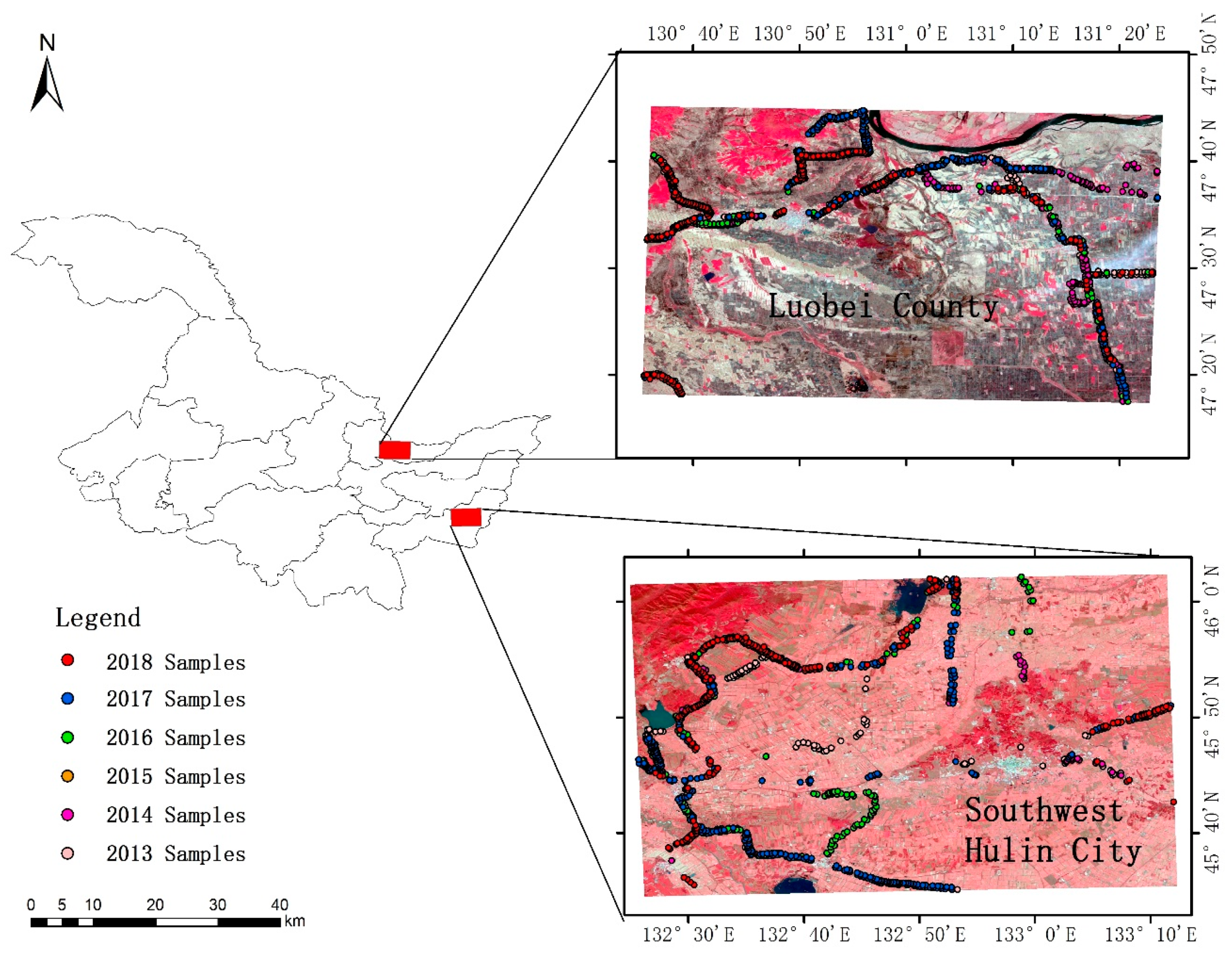
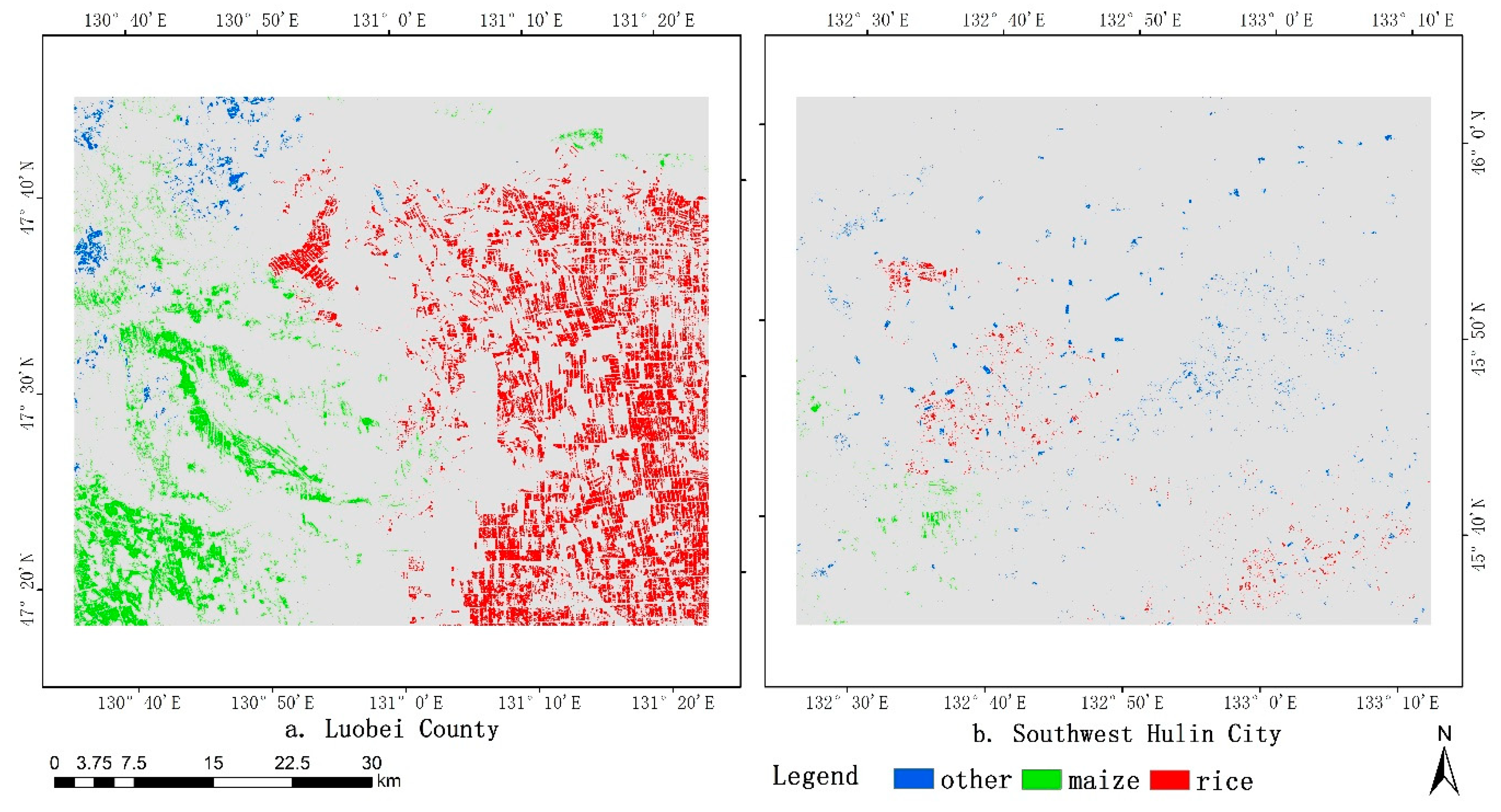
2.1. Study Area
2.2. Data Sources
2.2.1. Remote Sensing Data
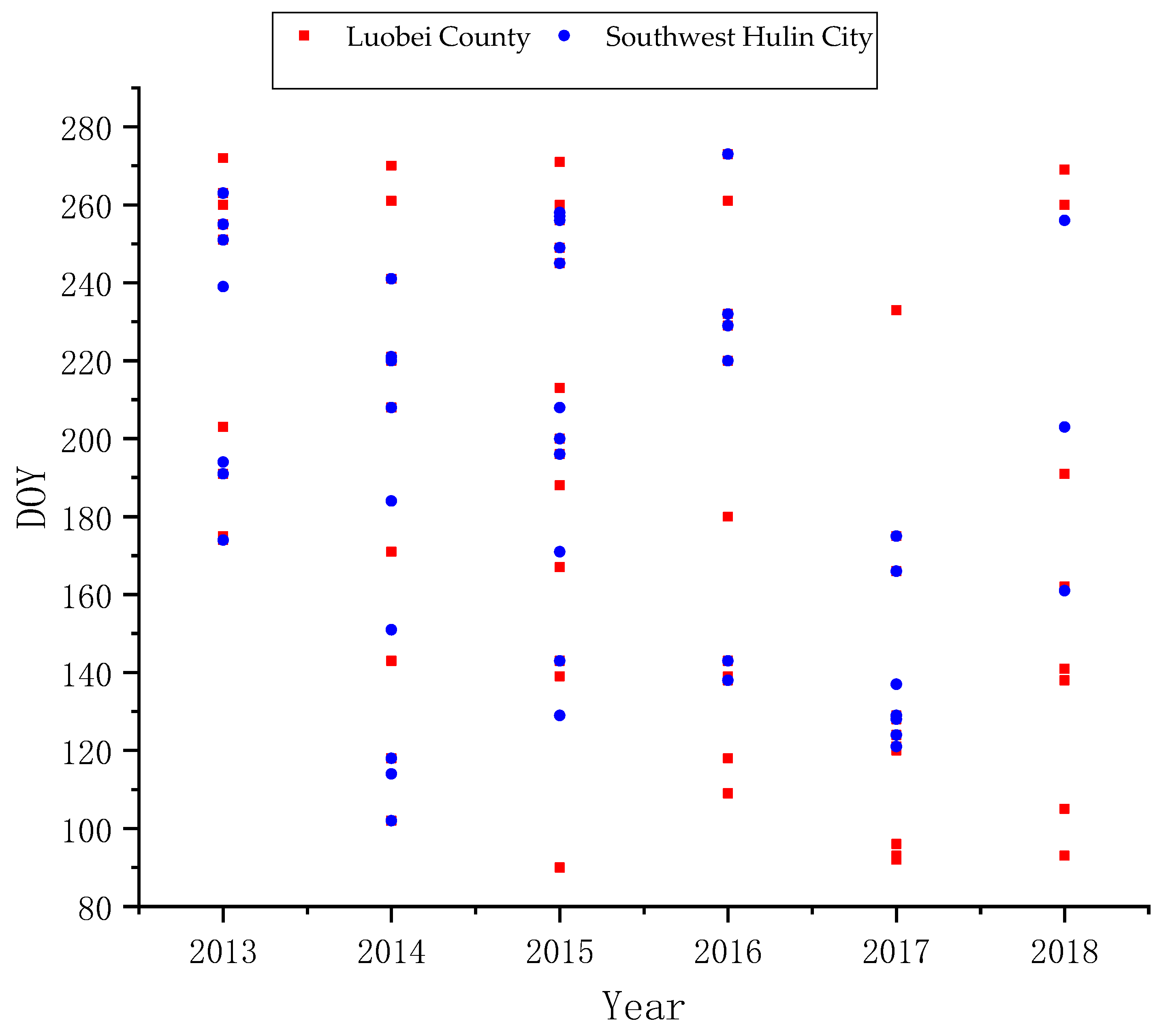
2.2.2. Field Sample Data
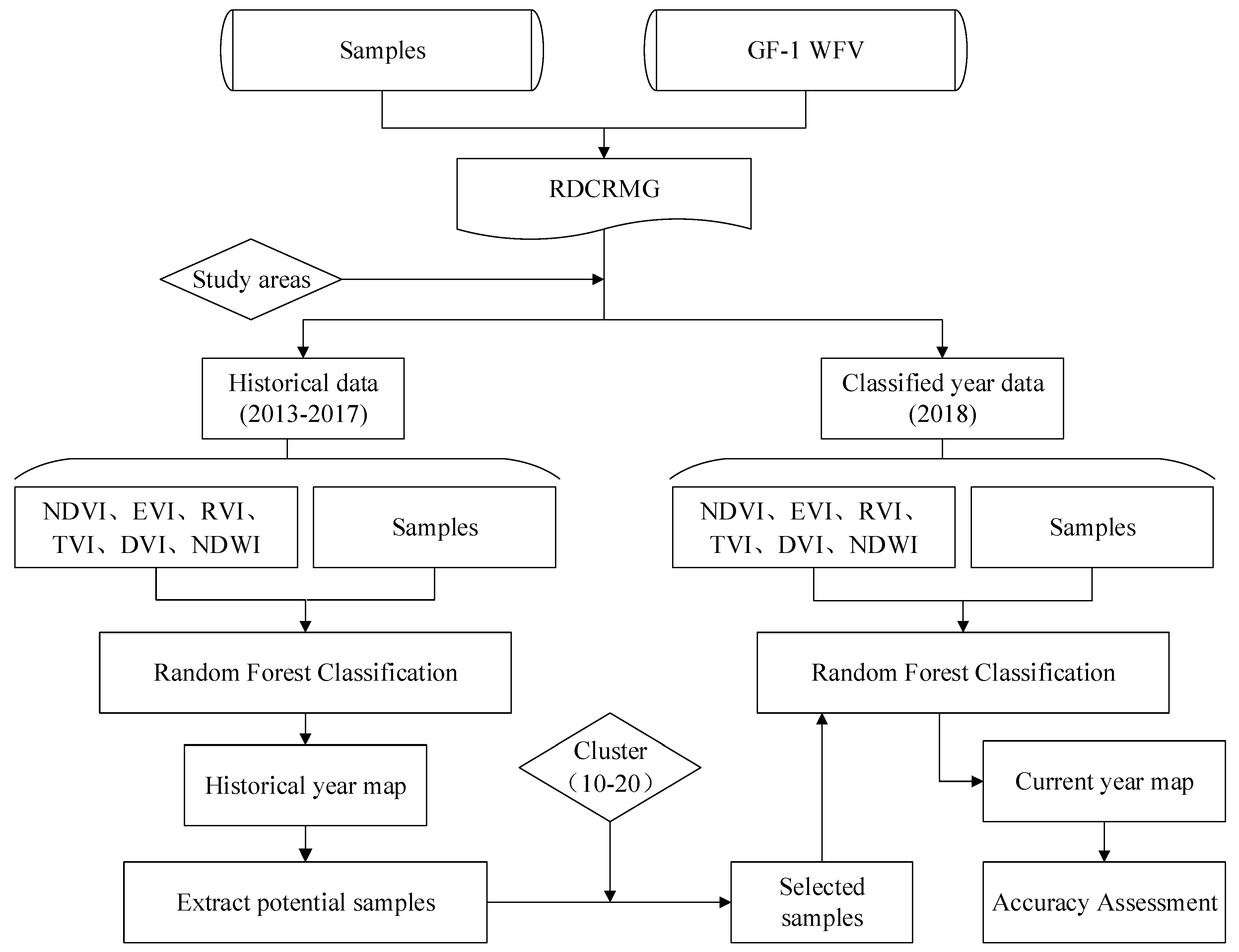
3. Methods
3.1. Data Preprocessing
3.2. Historical Year Crop Classification and Sampling Procedures
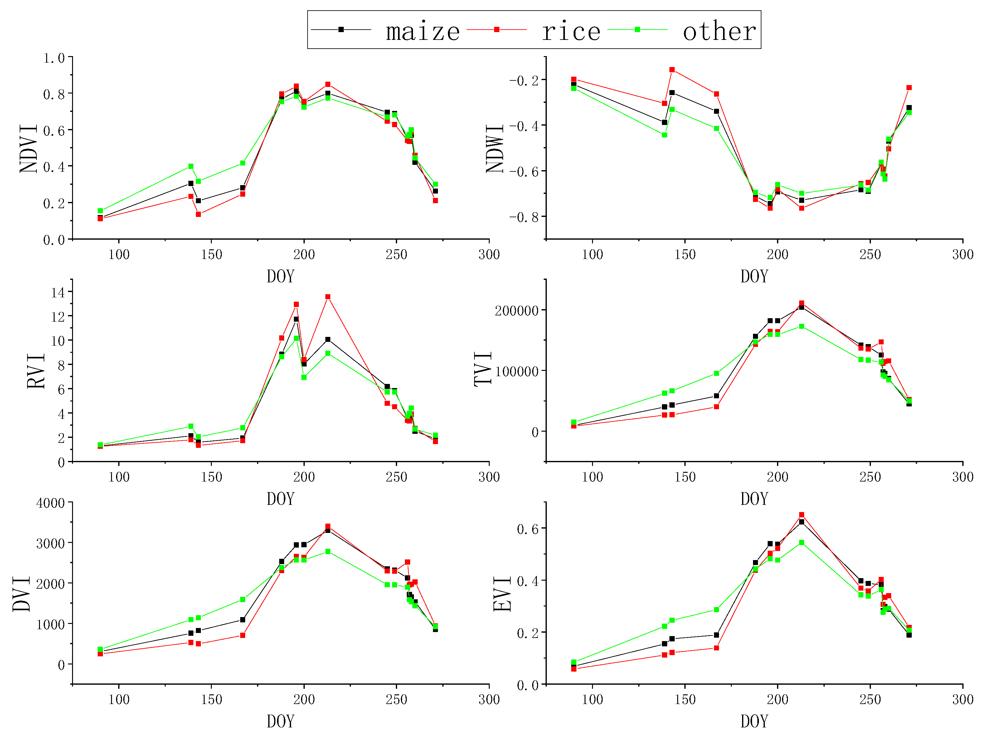
3.3. Classification Feature Selection and Calculation
3.4. Random Forest Classification
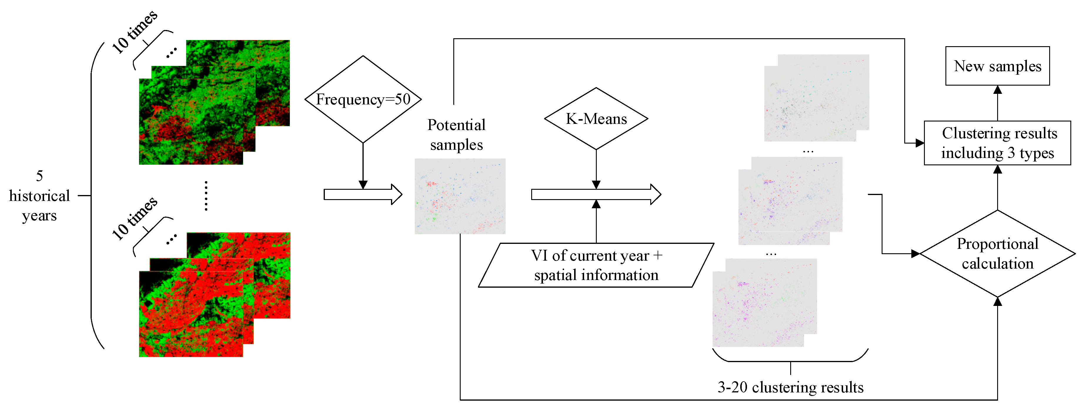
3.5. New Sample Generation and Screening
3.6. Accuracy Assessment
4. Results
4.1. Classification Results of Historical Years and Potential Sample Extraction
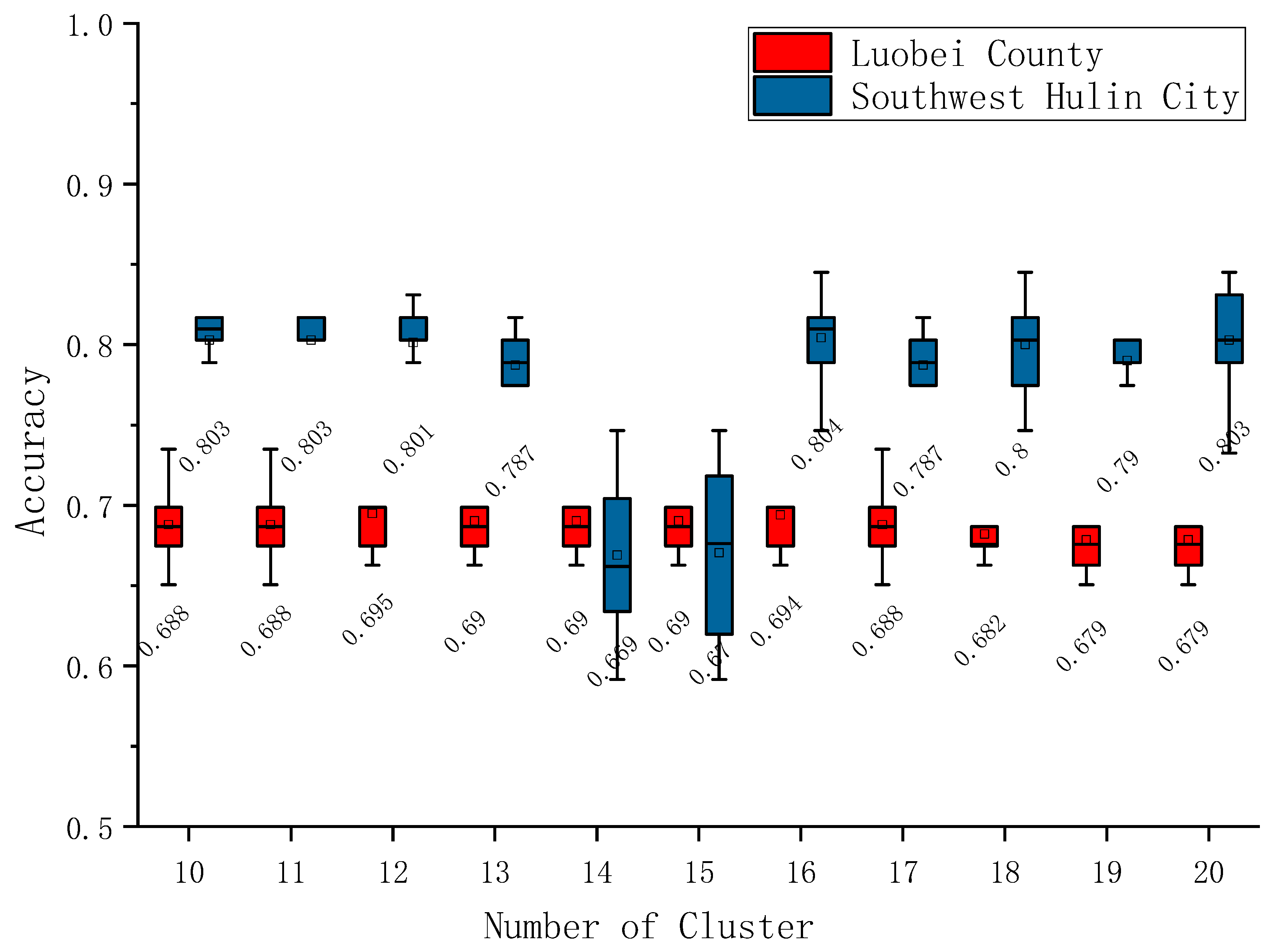
4.2. Effect of Clustering Number on New Sample Structure and Classification Accuracy
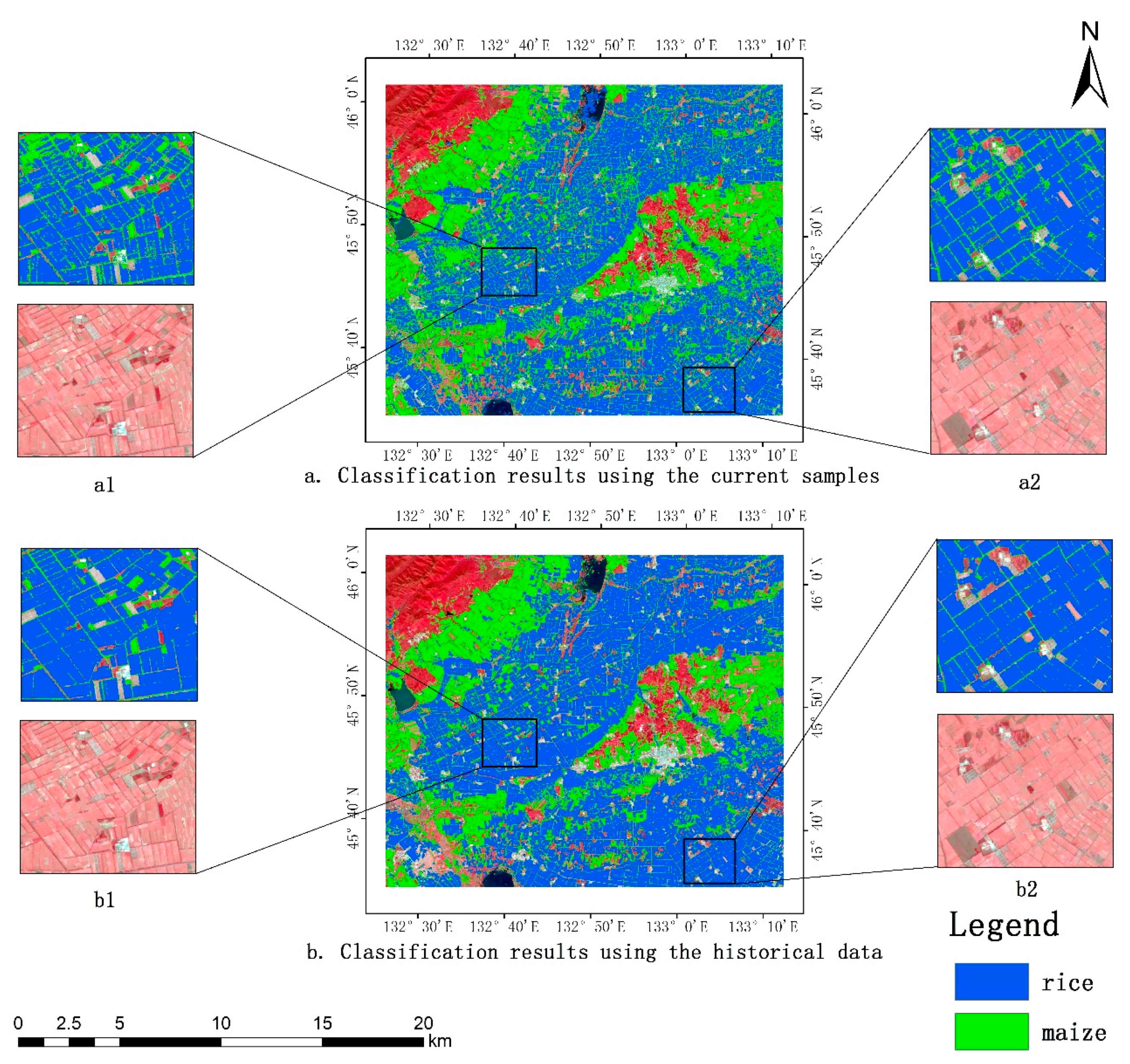
4.3. Accuracy Assessment and Analysis
5. Discussion
6. Conclusions
Author Contributions
Funding
Conflicts of Interest
References
- Hao, P.; Zhan, Y.; Wang, L.; Niu, Z.; Shakir, M. Feature Selection of Time Series MODIS Data for Early Crop Classification Using Random Forest: A Case Study in Kansas, USA. Remote Sens. 2015, 7, 5347–5369. [Google Scholar] [CrossRef] [Green Version]
- Doraiswamy, P.C.; Hatfield, J.L.; Jackson, T.J.; Akhmedov, B.; Prueger, J.; Stern, A. Crop condition and yield simulations using Landsat and MODIS. Remote Sens. Environ. 2004, 92, 548–559. [Google Scholar] [CrossRef]
- Haboudane, D.; Miller, J.R.; Tremblay, N.; Zarco-Tejada, P.J.; Dextraze, L. Integrated narrow-band vegetation indices for prediction of crop chlorophyll content for application to precision agriculture. Remote Sens. Environ. 2002, 81, 416–426. [Google Scholar] [CrossRef]
- Thenkabail, P.S.; Biradar, C.M.; Noojipady, P.; Dheeravath, V.; Li, Y.; Velpuri, M.; Gumma, M.; Gangalakunta, O.R.P.; Turral, H.; Cai, X.; et al. Global irrigated area map (GIAM), derived from remote sensing, for the end of the last millennium. Int. J. Remote Sens. 2009, 30, 3679–3733. [Google Scholar] [CrossRef]
- Huang, J.; Ma, H.; Su, W.; Zhang, X.; Huang, Y.; Fan, J.; Wu, W. Jointly Assimilating MODIS LAI and ET Products Into the SWAP Model for Winter Wheat Yield Estimation. IEEE J.-Stars. 2015, 8, 4060–4071. [Google Scholar] [CrossRef]
- Song, X.; Potapov, P.V.; Krylov, A.; King, L.; Di Bella, C.M.; Hudson, A.; Khan, A.; Adusei, B.; Stehman, S.V.; Hansen, M.C. National-scale soybean mapping and area estimation in the United States using medium resolution satellite imagery and field survey. Remote Sens. Environ. 2017, 190, 383–395. [Google Scholar] [CrossRef]
- Rudorff, B.F.T.; Sugawara, L.M.; Adami, M.; Freitas, R.M.; Aguiar, D.A.; Mello, M.P. Remote Sensing Time Series to Evaluate Direct Land Use Change of Recent Expanded Sugarcane Crop in Brazil. Sustainability 2012, 4, 574–585. [Google Scholar] [CrossRef] [Green Version]
- Belgiu, M.; Csillik, O. Sentinel-2 cropland mapping using pixel-based and object-based time-weighted dynamic time warping analysis. Remote Sens. Environ. 2018, 204, 509–523. [Google Scholar] [CrossRef]
- Wardlow, B.D.; Egbert, S.L.; Kastens, J.H. Analysis of time-series MODIS 250 m vegetation index data for crop classification in the U.S. Central Great Plains. Remote Sens. Environ. 2007, 108, 290–310. [Google Scholar] [CrossRef] [Green Version]
- Chen, Y.; Lu, D.; Moran, E.; Batistella, M.; Dutra, L.V.; Sanches, I.D.; Bicudo Da Silva, R.F.; Huang, J.; Barreto Luiz, A.J.; Falcao De Oliveira, M.A. Mapping croplands, cropping patterns, and crop types using MODIS time-series data. Int. J. Appl. Earth Obs. 2018, 69, 133–147. [Google Scholar] [CrossRef]
- Yang, N.; Liu, D.; Feng, Q.; Xiong, Q.; Zhang, L.; Ren, T.; Zhao, Y.; Zhu, D.; Huang, J. Large-Scale Crop Mapping Based on Machine Learning and Parallel Computation with Grids. Remote Sens. 2019, 11, 1500. [Google Scholar] [CrossRef]
- Brown, J.C.; Kastens, J.H.; Coutinho, A.C.; Victoria, D.D.C.; Bishop, C.R. Classifying multiyear agricultural land use data from Mato Grosso using time-series MODIS vegetation index data. Remote Sens. Environ. 2013, 130, 39–50. [Google Scholar] [CrossRef] [Green Version]
- Massey, R.; Sankey, T.T.; Congalton, R.G.; Yadav, K.; Thenkabail, P.S.; Ozdogan, M.; Sánchez Meador, A.J. MODIS phenology-derived, multi-year distribution of conterminous U.S. crop types. Remote Sens. Environ. 2017, 198, 490–503. [Google Scholar] [CrossRef]
- Sakamoto, T.; Wardlow, B.D.; Gitelson, A.A.; Verma, S.B.; Suyker, A.E.; Arkebauer, T.J. A Two-Step Filtering approach for detecting maize and soybean phenology with time-series MODIS data. Remote Sens. Environ. 2010, 114, 2146–2159. [Google Scholar] [CrossRef]
- Liu, J.; Huffman, T.; Shang, J.; Qian, B.; Dong, T.; Zhang, Y. Identifying Major Crop Types in Eastern Canada Using a Fuzzy Decision Tree Classifier and Phenological Indicators Derived from Time Series MODIS Data. Can. J. Remote Sens. 2016, 42, 259–273. [Google Scholar] [CrossRef]
- Pan, Z.; Huang, J.; Zhou, Q.; Wang, L.; Cheng, Y.; Zhang, H.; Blackburn, G.A.; Yan, J.; Liu, J. Mapping crop phenology using NDVI time-series derived from HJ-1 A/B data. Int. J. Appl. Earth Obs. 2015, 34, 188–197. [Google Scholar] [CrossRef]
- Roy, D.P.; Yan, L. Robust Landsat-based crop time series modelling. Remote Sens. Environ. 2018, 110810. [Google Scholar] [CrossRef]
- Soudani, K.; le Maire, G.; Dufrêne, E.; François, C.; Delpierre, N.; Ulrich, E.; Cecchini, S. Evaluation of the onset of green-up in temperate deciduous broadleaf forests derived from Moderate Resolution Imaging Spectroradiometer (MODIS) data. Remote Sens. Environ. 2008, 112, 2643–2655. [Google Scholar] [CrossRef]
- Zhong, L.; Hawkins, T.; Biging, G.; Gong, P. A phenology-based approach to map crop types in the San Joaquin Valley, California. Int. J. Remote Sens. 2011, 32, 7777–7804. [Google Scholar] [CrossRef]
- Zhong, L.; Gong, P.; Biging, G.S. Phenology-based Crop Classification Algorithm and its Implications on Agricultural Water Use Assessments in California’s Central Valley. Photogramm. Eng. Remote Sens. 2012, 78, 799–813. [Google Scholar] [CrossRef]
- Wu, W.; Yang, P.; Tang, H.; Zhou, Q.; Chen, Z.; Shibasaki, R. Characterizing Spatial Patterns of Phenology in Cropland of China Based on Remotely Sensed Data. Agric. Sci. China 2010, 9, 101–112. [Google Scholar] [CrossRef]
- Zheng, H.; Cheng, T.; Yao, X.; Deng, X.; Tian, Y.; Cao, W.; Zhu, Y. Detection of rice phenology through time series analysis of ground-based spectral index data. Field Crops Res. 2016, 198, 131–139. [Google Scholar] [CrossRef]
- Hao, P.; Wang, L.; Zhan, Y.; Niu, Z. Using Moderate-Resolution Temporal NDVI Profiles for High-Resolution Crop Mapping in Years of Absent Ground Reference Data: A Case Study of Bole and Manas Counties in Xinjiang, China. ISPRS Int. J. Geo-Inf. 2016, 5, 67. [Google Scholar] [CrossRef]
- Zhong, L.; Gong, P.; Biging, G.S. Efficient corn and soybean mapping with temporal extendability: A multi-year experiment using Landsat imagery. Remote Sens. Environ. 2014, 140, 1–13. [Google Scholar] [CrossRef]
- Zhong, L.; Hu, L.; Yu, L.; Gong, P.; Biging, G.S. Automated mapping of soybean and corn using phenology. ISPRS J. Photogramm. 2016, 119, 151–164. [Google Scholar] [CrossRef] [Green Version]
- Muhammad, S.; Zhan, Y.; Wang, L.; Hao, P.; Niu, Z. Major crops classification using time series MODIS EVI with adjacent years of ground reference data in the US state of Kansas. Optik 2016, 127, 1071–1077. [Google Scholar] [CrossRef]
- Cai, Y.; Guan, K.; Peng, J.; Wang, S.; Seifert, C.; Wardlow, B.; Li, Z. A high-performance and in-season classification system of field-level crop types using time-series Landsat data and a machine learning approach. Remote Sens. Environ. 2018, 210, 35–47. [Google Scholar] [CrossRef]
- Wang, S.; Azzari, G.; Lobell, D.B. Crop type mapping without field-level labels: Random forest transfer and unsupervised clustering techniques. Remote Sens. Environ. 2019, 222, 303–317. [Google Scholar] [CrossRef]
- Luciano, A.C.D.S.; Picoli, M.C.A.; Rocha, J.V.; Franco, H.C.J.; Sanches, G.M.; Leal, M.R.L.V.; le Maire, G. Generalized space-time classifiers for monitoring sugarcane areas in Brazil. Remote Sens. Environ. 2018, 215, 438–451. [Google Scholar] [CrossRef]
- Hao, P.; Wang, L.; Zhan, Y.; Wang, C.; Niu, Z.; Wu, M. Crop classification using crop knowledge of the previous-year: Case study in Southwest Kansas, USA. Eur. J. Remote Sens. 2016, 49, 1061–1077. [Google Scholar] [CrossRef]
- Zan, X.; Zhao, Z.; Liu, W.; Zhang, X.; Liu, Z.; Li, S.; Zhu, D. The Layout of Maize Variety Test Sites Based on the Spatiotemporal Classification of the Planting Environment. Sustainability 2019, 11, 3741. [Google Scholar] [CrossRef]
- Huang, N.; Liu, D.; Wang, Z.; Song, K.; Zhang, B.; Li, F.; Ren, C. Process of Transformation from Wetland to Farmland and Driving Mechanism Analysis in Luobei County of Sanjiang Plain. J. Geo-Inf. Sci. 2009, 11, 382–389. [Google Scholar] [CrossRef]
- Yang, J.; Lei, G. An Evaluation Study on Comprehensive Benefits of Land Use of Jixi Coal City in Heilongjiang Province. Res. Soil Water Conserv. 2012, 19, 176–179. [Google Scholar]
- Ye, S.; Liu, D.; Yao, X.; Tang, H.; Xiong, Q.; Zhuo, W.; Du, Z.; Huang, J.; Su, W.; Shen, S.; et al. RDCRMG: A Raster Dataset Clean & Reconstitution Multi-Grid Architecture for Remote Sensing Monitoring of Vegetation Dryness. Remote Sens. 2018, 10, 1376. [Google Scholar] [Green Version]
- Chen, D.M.; Stow, D. The effect of training strategies on supervised classification at different spatial resolutions. Photogramm. Eng. Remote Sens. 2002, 68, 1155–1161. [Google Scholar]
- Zhang, C.; Tong, L.; Liu, Z.; Qiao, M.; Liu, D.; Huang, J. Identification method of seed maize plot based on multi-temporal GF-1 WFV and kompsat-3 texture. Trans. Chin. Soc. Agric. Mach. 2019, 50, 163–168. [Google Scholar]
- Liu, J.; Feng, Q.; Gong, J.; Zhou, J.; Liang, J.; Li, Y. Winter wheat mapping using a random forest classifier combined with multi-temporal and multi-sensor data. Int. J. Digit. Earth 2018, 11, 783–802. [Google Scholar] [CrossRef]
- Tatsumi, K.; Yamashiki, Y.; Canales Torres, M.A.; Taipe, C.L.R. Crop classification of upland fields using Random forest of time-series Landsat 7 ETM+ data. Comput. Electron. Agric. 2015, 115, 171–179. [Google Scholar] [CrossRef]


| Year | Luobei County | Southwest Hulin City | ||||||
|---|---|---|---|---|---|---|---|---|
| Maize | Rice | Other | Total | Maize | Rice | Other | Total | |
| 2013 | 224 | 102 | 58 | 384 | 77 | 17 | 162 | 256 |
| 2014 | 284 | 146 | 123 | 553 | 131 | 36 | 75 | 242 |
| 2015 | 234 | 91 | 50 | 375 | 163 | 105 | 47 | 315 |
| 2016 | 234 | 91 | 49 | 374 | 146 | 102 | 45 | 293 |
| 2017 | 137 | 99 | 160 | 396 | 111 | 194 | 150 | 455 |
| 2018 | 128 | 32 | 78 | 237 | 122 | 37 | 47 | 206 |
| Year | Luobei County | Southwestern of Hulin City | ||||||
|---|---|---|---|---|---|---|---|---|
| Maize | Rice | Other | Total | Maize | Rice | Other | Total | |
| 2013 | 75 | 34 | 19 | 128 | 26 | 6 | 54 | 85 |
| 2014 | 95 | 49 | 41 | 184 | 44 | 12 | 25 | 81 |
| 2015 | 78 | 30 | 17 | 125 | 54 | 35 | 16 | 105 |
| 2016 | 78 | 30 | 16 | 125 | 49 | 34 | 15 | 98 |
| 2017 | 46 | 33 | 53 | 132 | 37 | 65 | 50 | 152 |
| 2018 | 43 | 11 | 26 | 79 | 41 | 12 | 16 | 69 |
| Luobei County | Southwest Hulin City | ||
|---|---|---|---|
| 2013 | Overall Accuracy (OA) | 85.77% ± 2.69% | 85.06% ± 4.60% |
| F-Score of Maize | 89.55% ± 2.28% | 76.31% ± 8.31% | |
| F-Score of Rice | 87.78% ± 3.40% | 76.15% ± 16.15% | |
| 2014 | OA | 87.17% ± 2.67% | 86.42% ± 6.17% |
| F-Score of Maize | 88.74% ± 2.45% | 88.64% ± 4.55% | |
| F-Score of Rice | 88.93% ± 2.91% | 90.00% ± 10.00% | |
| 2015 | OA | 86.22% ± 4.33% | 88.68% ± 3.77% |
| F-Score of Maize | 89.81% ± 2.96% | 89.57% ± 4.12% | |
| F-Score of Rice | 89.28% ± 5.64% | 94.50% ± 4.09% | |
| 2016 | OA | 85.32% ± 2.78% | 80.50% ± 5.50% |
| F-Score of Maize | 89.04% ± 1.98% | 82.15% ± 5.23% | |
| F-Score of Rice | 88.60% ± 4.73% | 88.11% ± 5.04% | |
| 2017 | OA | 76.49% ± 2.61% | 81.91% ± 3.62% |
| F-Score of Maize | 75.80% ± 3.80% | 70.97% ± 6.18% | |
| F-Score of Rice | 82.66% ± 5.47% | 91.04% ± 5.93% |
| Luobei County | Southwest Hulin City | |||||
|---|---|---|---|---|---|---|
| Other | Maize | Rice | Other | Maize | Rice | |
| 10 | 3.93% | 33.91% | 62.16% | 52.91% | 16.04% | 31.05% |
| 11 | 3.94% | 33.86% | 62.21% | 70.54% | 15.56% | 13.90% |
| 12 | 3.97% | 30.01% | 66.02% | 54.31% | 14.58% | 31.11% |
| 13 | 3.97% | 30.01% | 66.02% | 54.89% | 14.18% | 30.93% |
| 14 | 3.97% | 30.01% | 66.02% | 51.15% | 9.08% | 39.77% |
| 15 | 3.97% | 30.01% | 66.02% | 51.55% | 8.95% | 39.50% |
| 16 | 3.97% | 29.97% | 66.06% | 47.81% | 14.76% | 37.43% |
| 17 | 3.84% | 35.72% | 60.44% | 50.39% | 12.30% | 37.31% |
| 18 | 3.71% | 36.44% | 59.85% | 48.46% | 14.42% | 37.13% |
| 19 | 3.44% | 26.44% | 70.12% | 48.62% | 14.42% | 36.96% |
| 20 | 3.44% | 26.44% | 70.12% | 48.57% | 14.48% | 36.95% |
| Predictive Value | ||||||||
|---|---|---|---|---|---|---|---|---|
| Other | Maize | Rice | Producer Accuracy (PA) (%) | Other | Maize | Rice | PA (%) | |
| South of Luobei County | Southwest Hulin City | |||||||
| Using Sample of 2018, OA: 77.59%, Kappa: 0.61 | Using Sample of 2018, OA: 82.94%, Kappa: 0.71 | |||||||
| Other | 20 | 7 | 0 | 72.22% | 11 | 4 | 1 | 67.36% |
| Maize | 6 | 38 | 1 | 85.23% | 4 | 37 | 1 | 89.15% |
| Rice | 0 | 4 | 7 | 61.67% | 2 | 1 | 11 | 82.05% |
| User Accuracy (UA) (%) | 76.77% | 76.53% | 86.05% | 65.54% | 88.22% | 88.07% | ||
| Using sample of historical data, OA: 69.35%, Kappa: 0.42 | Using sample of historical data, OA: 80.44%, Kappa: 0.65 | |||||||
| Other | 8 | 19 | 0 | 28.89% | 10 | 6 | 0 | 59.72% |
| Maize | 1 | 42 | 1 | 94.78% | 5 | 37 | 1 | 87.04% |
| Rice | 1 | 3 | 8 | 66.91% | 2 | 0 | 11 | 84.62% |
| UA (%) | 80.78% | 65.31% | 85.11% | 58.90% | 85.01% | 63.40% | ||
© 2019 by the authors. Licensee MDPI, Basel, Switzerland. This article is an open access article distributed under the terms and conditions of the Creative Commons Attribution (CC BY) license (http://creativecommons.org/licenses/by/4.0/).
Share and Cite
Zhang, L.; Liu, Z.; Liu, D.; Xiong, Q.; Yang, N.; Ren, T.; Zhang, C.; Zhang, X.; Li, S. Crop Mapping Based on Historical Samples and New Training Samples Generation in Heilongjiang Province, China. Sustainability 2019, 11, 5052. https://0-doi-org.brum.beds.ac.uk/10.3390/su11185052
Zhang L, Liu Z, Liu D, Xiong Q, Yang N, Ren T, Zhang C, Zhang X, Li S. Crop Mapping Based on Historical Samples and New Training Samples Generation in Heilongjiang Province, China. Sustainability. 2019; 11(18):5052. https://0-doi-org.brum.beds.ac.uk/10.3390/su11185052
Chicago/Turabian StyleZhang, Lin, Zhe Liu, Diyou Liu, Quan Xiong, Ning Yang, Tianwei Ren, Chao Zhang, Xiaodong Zhang, and Shaoming Li. 2019. "Crop Mapping Based on Historical Samples and New Training Samples Generation in Heilongjiang Province, China" Sustainability 11, no. 18: 5052. https://0-doi-org.brum.beds.ac.uk/10.3390/su11185052