Evaluating Agricultural Sustainability Based on the Water–Energy–Food Nexus in the Chenmengquan Irrigation District of China


Abstract
:1. Introduction
2. Case Study
3. Methods
3.1. Index System
3.1.1. Water
3.1.2. Energy
3.1.3. Food
3.2. Calculation of the Weights
3.2.1. The G1 Method
3.2.2. The Entropy Method
3.2.3. Combination Weighting Rule
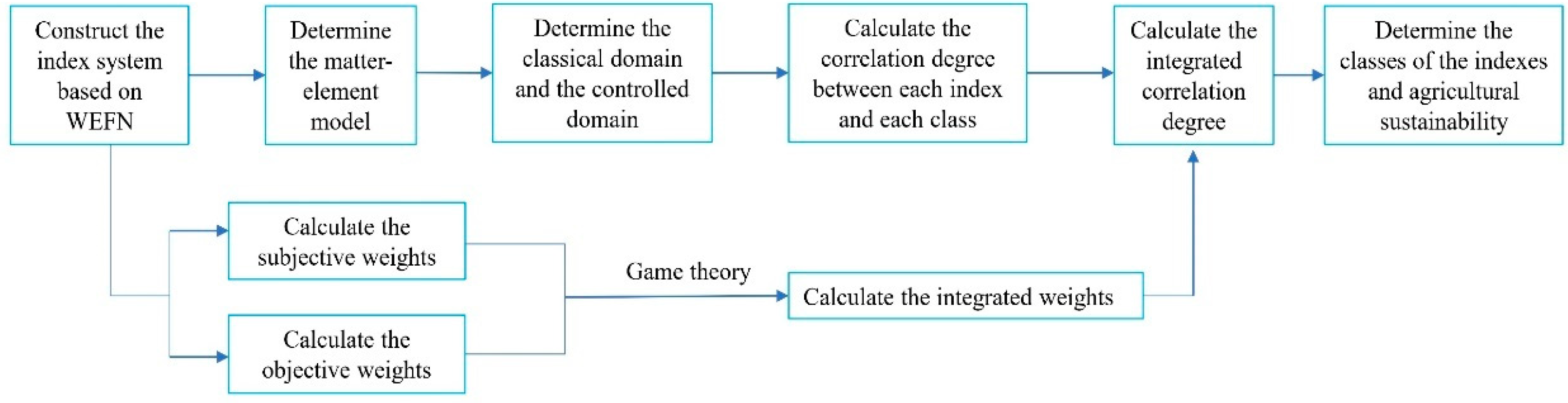
3.3. Matter–Element Model
3.3.1. Determining the Matter–Element
3.3.2. Determining the Classical Domain and the Controlled Domain Matter–Element Matrix
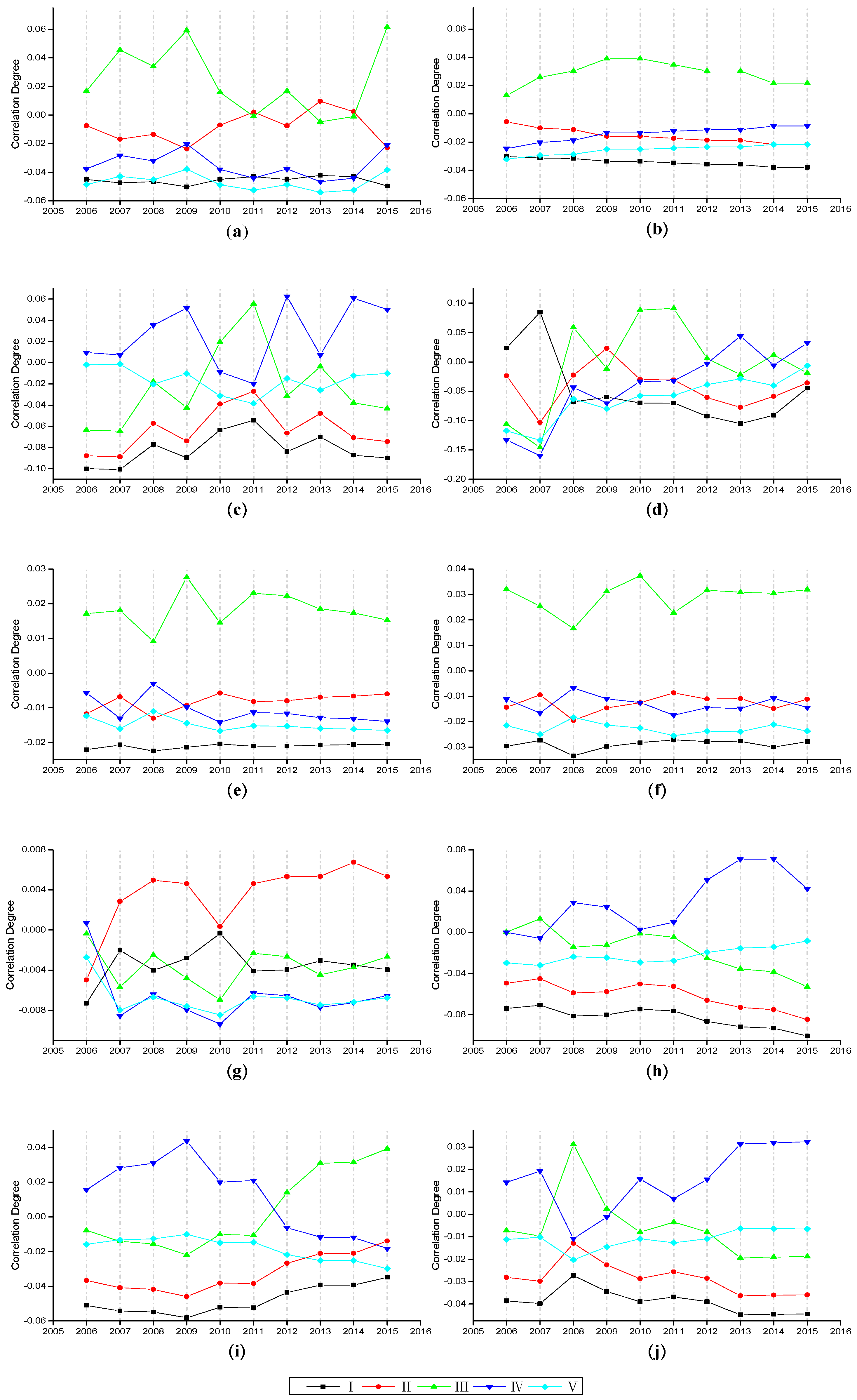
3.3.3. Correlation Degree between Each Index and Each Class
4. Results
4.1. The Weights of Indexes
4.2. The Classical Domain and the Controlled Domain
4.3. Determination of the Sustainability Class
5. Analysis and Discussion
6. Conclusions
Author Contributions
Funding
Conflicts of Interest
References
- Agathokleous, E.; Calabrese, E.J. Hormesis can enhance agricultural sustainability in a changing world. Global Food Sec. 2019, 20, 150–155. [Google Scholar] [CrossRef]
- FAO. Climate-Smart Agriculture Sourcebook. Available online: http://www.fao.org/3/i3325e/i3325e.pdf (accessed on 22 September 2019).
- FAO. The State of World’s Land and Water Resources for Food and Agriculture. Available online: http://www.fao.org/docrep/017/i1688e/i1688e.pdf (accessed on 22 September 2019).
- Xue, J.; Huo, Z.; Huang, Q.; Wang, F.; Boll, J.; Huang, G.; Qu, Z. Assessing sustainability of agricultural water saving in an arid area with shallow groundwater. Irrig. Drain. 2019, 68, 205–217. [Google Scholar] [CrossRef]
- Byomkesh, T.; Blay-Palmer, A. Comparison of Methods to Assess Agricultural Sustainability. In Sustainable Agriculture Reviews 13; Springer: Cham, Switzerland, 2017. [Google Scholar]
- Gomez-Limon, J.A.; Sanchez-Fernandez, G. Empirical evaluation of agricultural sustainability using composite indicators. Ecol. Econ. 2010, 69, 1062–1075. [Google Scholar] [CrossRef]
- Kamali, F.P.; Borges, J.A.R.; Meuwissen, M.P.M.; de Boer, I.J.M.; Lansink, A. Sustainability assessment of agricultural systems: The validity of expert opinion and robustness of a multi-criteria analysis. Agric. Syst. 2017, 157, 118–128. [Google Scholar] [CrossRef]
- Talukder, B.; Blay-Palmer, A.; Hipel, K.; Van Loon, G. Elimination Method of Multi-Criteria Decision Analysis (MCDA): A Simple Methodological Approach for Assessing Agricultural Sustainability. Sustainability 2017, 9, 287. [Google Scholar] [CrossRef]
- Bertocchi, M.; Demartini, E.; Marescotti, M.E. Ranking farms using quantitative indicators of sustainability: The 4Agro method. In 2nd International Symposium New Metropolitan Perspectives—Strategic Planning, Spatial Planning, Economic Programs and Decision Support Tools, through the Implementation of Horizon/Europe 2020; Calabro, F., Della Spina, L., Eds.; Elsevier Science Bv: Amsterdam, The Netherlands, 2016; pp. 726–732. [Google Scholar]
- Talukder, B.; Hipel, K.W. The PROMETHEE Framework for Comparing the Sustainability of Agricultural Systems. Resources 2018, 7, 74. [Google Scholar] [CrossRef]
- Van Cauwenbergh, N.; Biala, K.; Bielders, C.; Brouckaert, V.; Franchois, L.; Cidad, V.G.; Hermy, M.; Mathijs, E.; Muys, B.; Reijnders, J.; et al. SAFE—A hierarchical framework for assessing the sustainability of agricultural systems. Agric. Ecosyst. Environ. 2007, 120, 229–242. [Google Scholar] [CrossRef]
- Wohlfender-Bühler, D.; Feusthuber, E.; Wäger, R.; Mann, S.; Aubry, S.J. Genetically modified crops in Switzerland: Implications for agrosystem sustainability evidenced by multi-criteria model. Agron. Sustain. Dev. 2016, 36, 33. [Google Scholar] [CrossRef]
- Von Wiren-Lehr, S. Sustainability in agriculture—An evaluation of principal goal-oriented concepts to close the gap between theory and practice. Agric. Ecosyst. Environ. 2001, 84, 115–129. [Google Scholar] [CrossRef]
- Hoff, H. Understanding the Nexus: Background Paper for the BONN2011 Nexus Conference; SEI: Stockholm, Sweden, 2011; 51p. [Google Scholar]
- Li, M.; Fu, Q.; Singh, V.P.; Ji, Y.; Liu, D.; Zhang, C.; Li, T. An optimal modelling approach for managing agricultural water-energy-food nexus under uncertainty. Sci. Total Environ. 2019, 651, 1416–1434. [Google Scholar] [CrossRef]
- FAO. Walking the Nexus Talk: Assessing the Water-Energy-Food Nexus. Available online: http://www.fao.org/3/a-i3959e.pdf (accessed on 22 September 2019).
- Smajgl, A.; Ward, J.; Pluschke, L. The water-food-energy Nexus—Realising a new paradigm. J. Hydrol. 2016, 533, 533–540. [Google Scholar] [CrossRef]
- Han, H.; Li, H.; Zhang, K. Urban Water Ecosystem Health Evaluation Based on the Improved Fuzzy Matter-Element Extension Assessment Model: Case Study from Zhengzhou City, China. Math. Prob. Eng. 2019, 2019, 1–14. [Google Scholar] [CrossRef]
- Gebler, D.; Wiegleb, G.; Szoszkiewicz, K. Integrating river hydromorphology and water quality into ecological status modelling by artificial neural networks. Water Res. 2018, 139, 395–405. [Google Scholar] [CrossRef] [PubMed]
- Sun, D.; Wu, J.; Zhang, F.; Su, W.; Hui, H. Evaluating Water Resource Security in Karst Areas Using DPSIRM Modeling, Gray Correlation, and Matter-Element Analysis. Sustainability 2018, 10, 3934. [Google Scholar] [CrossRef]
- Qian, C.; Zhang, M.; Chen, Y.; Wang, R. A Quantitative Judgement Method for Safety Admittance of Facilities in Chemical Industrial Parks based on G1-Variation Coefficient Method. Procedia Eng. 2014, 84, 223–232. [Google Scholar] [CrossRef] [Green Version]
- Shemshadi, A.; Shirazi, H.; Toreihi, M.; Tarokh, M.J. A fuzzy VIKOR method for supplier selection based on entropy measure for objective weighting. Expert Syst. Applic. 2011, 38, 12160–12167. [Google Scholar] [CrossRef]
- Dong, L.; Gu, X.; Wu, X.; Liao, H. An improved MULTIMOORA method with combined weights and its application in assessing the innovative ability of universities. Expert Syst. 2019, 36, e12362. [Google Scholar] [CrossRef]
- Wen, C.; Dong, W.; Meng, Y.; Li, C.; Zhang, Q. Application of a loose coupling model for assessing the impact of land-cover changes on groundwater recharge in the Jinan spring area, China. Environ. Earth Sci. 2019, 78, 13. [Google Scholar] [CrossRef]
- Cao, X.; Ren, J.; Wu, M.; Guo, X.; Wang, Z.; Wang, W. Effective use rate of generalized water resources assessment and to improve agricultural water use efficiency evaluation index system. Ecol. Indic. 2018, 86, 58–66. [Google Scholar] [CrossRef]
- Hoekstra, A.Y.; Mekonnen, M.M. The water footprint of humanity. Proc. Natl. Acad. Sci. USA 2012, 109, 3232. [Google Scholar] [CrossRef]
- Pachauri, S.; Spreng, D. Direct and indirect energy requirements of households in India. Energy Policy 2002, 30, 511–523. [Google Scholar] [CrossRef]
- De Vito, R.; Portoghese, I.; Pagano, A.; Fratino, U.; Vurro, M. An index-based approach for the sustainability assessment of irrigation practice based on the water-energy-food nexus framework. Adv. Water Resour. 2017, 110, 423–436. [Google Scholar] [CrossRef]
- Daccache, A.; Ciurana, J.S.; Rodriguez Diaz, J.A.; Knox, J.W. Water and energy footprint of irrigated agriculture in the Mediterranean region. Environ. Res. Lett. 2014, 9, 124014. [Google Scholar] [CrossRef]
- Wang, M.; Tang, D.; Bai, Y.; Xia, Z. A compound cloud model for harmoniousness assessment of water allocation. Environ. Earth Sci. 2016, 75, 11. [Google Scholar] [CrossRef]
- Talukder, B.; Hipel, K.W.; VanLoon, G.W. Developing Composite Indicators for Agricultural Sustainability Assessment: Effect of Normalization and Aggregation Techniques. Resources 2017, 6, 66. [Google Scholar] [CrossRef]
- Islam, A.R.M.T.; Ahmed, N.; Bodrud-Doza, M.; Chu, R. Characterizing groundwater quality ranks for drinking purposes in Sylhet district, Bangladesh, using entropy method, spatial autocorrelation index, and geostatistics. Environ. Sci.Pollut. Res. 2017, 24, 26350–26374. [Google Scholar] [CrossRef] [PubMed]
- Busing, F.M.T.A.; Groenen, P.J.K.; Heiser, W.J. Avoiding degeneracy in multidimensional unfolding by penalizing on the coefficient of variation. Psychometrika 2005, 70, 71–98. [Google Scholar] [CrossRef]
- Pourghasemi, H.R.; Pradhan, B.; Gokceoglu, C. Application of fuzzy logic and analytical hierarchy process (AHP) to landslide susceptibility mapping at Haraz watershed, Iran. Nat. Hazards 2012, 63, 965–996. [Google Scholar] [CrossRef]
- Okoli, C.; Pawlowski, S.D. The Delphi method as a research tool: An example, design considerations and applications. Inf. Manag. 2004, 42, 15–29. [Google Scholar] [CrossRef]
- Zhang, W.; Chen, J.-P.; Wang, Q.; An, Y.; Qian, X.; Xiang, L.; He, L. Susceptibility analysis of large-scale debris flows based on combination weighting and extension methods. Nat. Hazards 2013, 66, 1073–1100. [Google Scholar] [CrossRef]
- Szeszlér, D. Hitting a path: A generalization of weighted connectivity via game theory. J. Combin. Optim. 2019, 38, 72–85. [Google Scholar] [CrossRef]
- Madani, K. Game theory and water resources. J. Hydrol. 2010, 381, 225–238. [Google Scholar] [CrossRef]
- Liu, D.; Zou, Z. Water quality evaluation based on improved fuzzy matter-element method. J. Environ. Sci. 2012, 24, 1210–1216. [Google Scholar] [CrossRef]
- He, Y.-X.; Dai, A.-Y.; Zhu, J.; He, H.-Y.; Li, F. Risk assessment of urban network planning in china based on the matter-element model and extension analysis. Int. J. Electric. Power Energy Syst. 2011, 33, 775–782. [Google Scholar] [CrossRef]
- Gong, J.; Liu, Y.; Chen, W. Land suitability evaluation for development using a matter-element model: A case study in Zengcheng, Guangzhou, China. Land Use Policy 2012, 29, 464–472. [Google Scholar] [CrossRef]
- Yang, R.; Cui, B.; Zhao, H.; Lei, X. An Integrated Act for Groundwater Protection of Jinan City, China. Procedia Environ. Sci. 2010, 2, 1745–1749. [Google Scholar] [CrossRef] [Green Version]
- Nemati, H.; Shokri, M.R.; Ramezanpour, Z.; Ebrahimi Pour, G.H.; Muxika, I.; Borja, Á. Sensitivity of indicators matters when using aggregation methods to assess marine environmental status. Mar. Poll. Bull. 2018, 128, 234–239. [Google Scholar] [CrossRef]
- Alvarez, M.C.; Franco, A.; Pérez-Domínguez, R.; Elliott, M. Sensitivity analysis to explore responsiveness and dynamic range of multi-metric fish-based indices for assessing the ecological status of estuaries and lagoons. Hydrobiologia 2013, 704, 347–362. [Google Scholar] [CrossRef]


| Sector | Index (unit) |
|---|---|
| Water | c1 Agricultural blue water proportion |
| c2 Water-use efficiency | |
| c3 Irrigation proportion of arable land | |
| Energy | c4 Energy utilization for irrigation amount per arable land (kWh/ha) |
| c5 Agricultural machinery power per arable land (kW/ha) | |
| c6 Fertilizer utilization amount per arable land(kg/ha) | |
| c7 Pesticide utilization amount per arable land(kg/ha) | |
| Food | c8 Yield per unit area of Wheat(t/ha) |
| c9 Yield per unit area of Maize(t/ha) | |
| c10 Yield per unit area of Vegetable(t/ha) |
| ri | Instruction |
|---|---|
| 1.0 | The index ci−1 and index ci are equally important |
| 1.2 | The index ci−1 is slightly more important than index ci |
| 1.4 | The index ci−1 is fairly more important than index ci |
| 1.6 | The index ci−1 is strongly more important than index ci |
| 2.0 | The index ci−1 is extremely more important than index ci |
| Index | c1 | c2 | c3 | c4 | c5 | c6 | c7 | c8 | c9 | c10 |
|---|---|---|---|---|---|---|---|---|---|---|
| wi1 | 0.095 | 0.114 | 0.079 | 0.137 | 0.079 | 0.114 | 0.114 | 0.095 | 0.079 | 0.095 |
| wi2 | 0.133 | 0.084 | 0.142 | 0.193 | 0.055 | 0.072 | 0.005 | 0.153 | 0.096 | 0.068 |
| wi | 0.13 | 0.087 | 0.137 | 0.188 | 0.057 | 0.075 | 0.014 | 0.148 | 0.094 | 0.07 |
| Index | The Classical Domain | The Controlled Domain | ||||
|---|---|---|---|---|---|---|
| Very Low | Low | Moderate | High | Very High | ||
| c1 | [0.8, 1] | [0.6, 0.8] | [0.4, 0.6] | [0.2, 0.4] | [0, 0.2] | [0, 1] |
| c2 | [0, 0.2] | [0.2, 0.4] | [0.4, 0.6] | [0.6, 0.8] | [0.8, 1] | [0, 1] |
| c3 | [0, 0.2] | [0.2, 0.4] | [0.4, 0.6] | [0.6, 0.8] | [0.8, 1] | [0, 1] |
| c4 | [1.6, 2] | [1.2, 1.6] | [0.8, 1.2] | [0.4, 0.8] | [0, 0.4] | [0, 2] |
| c5 | [25, 30] | [20, 25] | [15, 20] | [10, 15] | [0, 10] | [0, 30] |
| c6 | [800, 1000] | [600, 800] | [400, 600] | [200, 400] | [0, 200] | [0, 1000] |
| c7 | [16, 20] | [12, 16] | [8, 12] | [4, 8] | [0, 4] | [0, 20] |
| c8 | [2, 3] | [3, 4] | [4, 5] | [5, 6] | [6, 7] | [2, 7] |
| c9 | [3, 4] | [4, 5] | [5, 6] | [6, 7] | [7, 8] | [3, 8] |
| c10 | [30, 42] | [42, 54] | [54, 66] | [66, 78] | [78, 90] | [30, 90] |
| Index | Very Low | Low | Moderate | High | Very High | CLASSES |
|---|---|---|---|---|---|---|
| c1 | −0.050 | −0.023 | 0.062 | −0.021 | −0.038 | moderate |
| c2 | −0.038 | −0.022 | 0.022 | −0.009 | −0.022 | moderate |
| c3 | −0.090 | −0.074 | −0.043 | 0.050 | −0.010 | high |
| c4 | −0.111 | −0.085 | −0.034 | 0.069 | −0.024 | high |
| c5 | −0.020 | −0.006 | 0.015 | −0.014 | −0.017 | moderate |
| c6 | −0.028 | −0.011 | 0.032 | −0.014 | −0.024 | moderate |
| c7 | −0.004 | 0.005 | −0.003 | −0.007 | −0.007 | low |
| c8 | −0.100 | −0.085 | −0.053 | 0.042 | −0.008 | high |
| c9 | −0.035 | −0.014 | 0.039 | −0.018 | −0.030 | moderate |
| c10 | −0.044 | −0.036 | −0.019 | 0.032 | −0.006 | high |
| Index | 2006 | 2007 | 2008 | 2009 | 2010 | 2011 | 2012 | 2013 | 2014 | 2015 |
|---|---|---|---|---|---|---|---|---|---|---|
| c1 | Ⅲ | Ⅲ | Ⅲ | Ⅲ | Ⅲ | Ⅱ | Ⅲ | Ⅱ | Ⅱ | Ⅲ |
| c2 | Ⅲ | Ⅲ | Ⅲ | Ⅲ | Ⅲ | Ⅲ | Ⅲ | Ⅲ | Ⅲ | Ⅲ |
| c3 | Ⅳ | Ⅳ | Ⅳ | Ⅳ | Ⅲ | Ⅲ | Ⅳ | Ⅳ | Ⅳ | Ⅳ |
| c4 | Ⅰ | Ⅰ | Ⅲ | Ⅱ | Ⅲ | Ⅲ | Ⅲ | Ⅳ | Ⅲ | Ⅳ |
| c5 | Ⅲ | Ⅲ | Ⅲ | Ⅲ | Ⅲ | Ⅲ | Ⅲ | Ⅲ | Ⅲ | Ⅲ |
| c6 | Ⅲ | Ⅲ | Ⅲ | Ⅲ | Ⅲ | Ⅲ | Ⅲ | Ⅲ | Ⅲ | Ⅲ |
| c7 | Ⅳ | Ⅱ | Ⅱ | Ⅱ | Ⅱ | Ⅱ | Ⅱ | Ⅱ | Ⅱ | Ⅱ |
| c8 | Ⅲ | Ⅲ | Ⅳ | Ⅳ | Ⅳ | Ⅳ | Ⅳ | Ⅳ | Ⅳ | Ⅳ |
| c9 | Ⅳ | Ⅳ | Ⅳ | Ⅳ | Ⅳ | Ⅳ | Ⅲ | Ⅲ | Ⅲ | Ⅲ |
| c10 | Ⅳ | Ⅳ | Ⅲ | Ⅲ | Ⅳ | Ⅳ | Ⅳ | Ⅳ | Ⅳ | Ⅳ |
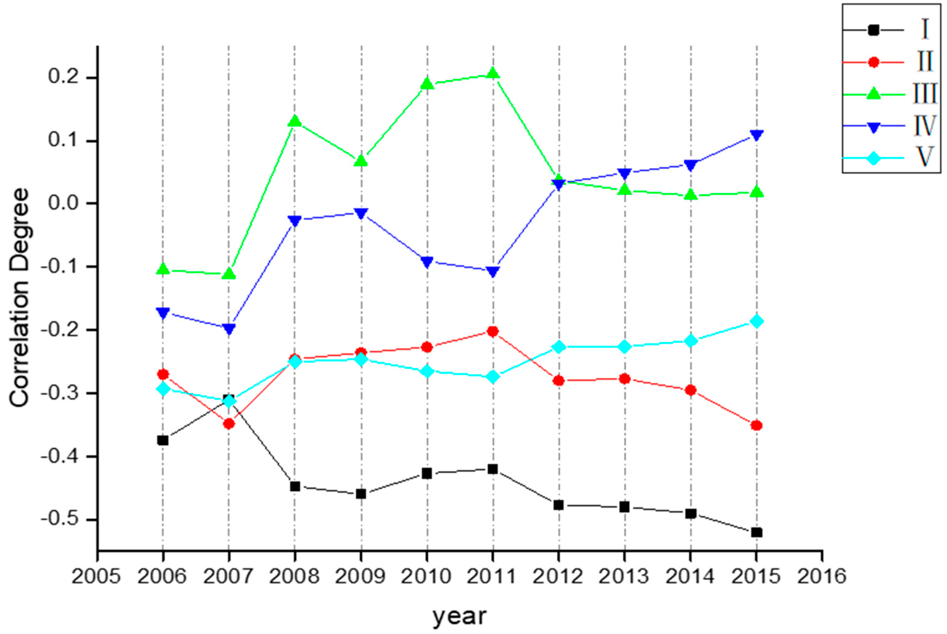
| Object | Very Low | Low | Moderate | High | Very High | Classes |
|---|---|---|---|---|---|---|
| 2006 | −0.374 | −0.270 | −0.105 | −0.172 | −0.293 | moderate |
| 2007 | −0.310 | −0.348 | −0.112 | −0.197 | −0.312 | moderate |
| 2008 | −0.447 | −0.246 | 0.130 | −0.026 | −0.250 | moderate |
| 2009 | −0.460 | −0.236 | 0.067 | −0.014 | −0.246 | moderate |
| 2010 | −0.427 | −0.227 | 0.189 | −0.091 | −0.265 | moderate |
| 2011 | −0.420 | −0.202 | 0.205 | −0.106 | −0.274 | moderate |
| 2012 | −0.477 | −0.28 | 0.0363 | 0.032 | −0.227 | moderate |
| 2013 | −0.480 | −0.277 | 0.021 | 0.049 | −0.226 | high |
| 2014 | −0.490 | −0.295 | 0.013 | 0.062 | −0.217 | high |
| 2015 | −0.521 | −0.351 | 0.018 | 0.110 | −0.186 | high |
| Index | Variation Range | ||||
|---|---|---|---|---|---|
| −5% | −10% | +5% | +10% | 0 | |
| c2 | III | III | III | IV | III |
| c8 | IV | IV | Ⅴ | Ⅴ | IV |
| c9 | III | II | III | III | III |
| c10 | IV | III | IV | Ⅴ | IV |
© 2019 by the authors. Licensee MDPI, Basel, Switzerland. This article is an open access article distributed under the terms and conditions of the Creative Commons Attribution (CC BY) license (http://creativecommons.org/licenses/by/4.0/).
Share and Cite
Liu, C.; Zhang, Z.; Liu, S.; Liu, Q.; Feng, B.; Tanzer, J. Evaluating Agricultural Sustainability Based on the Water–Energy–Food Nexus in the Chenmengquan Irrigation District of China. Sustainability 2019, 11, 5350. https://0-doi-org.brum.beds.ac.uk/10.3390/su11195350
Liu C, Zhang Z, Liu S, Liu Q, Feng B, Tanzer J. Evaluating Agricultural Sustainability Based on the Water–Energy–Food Nexus in the Chenmengquan Irrigation District of China. Sustainability. 2019; 11(19):5350. https://0-doi-org.brum.beds.ac.uk/10.3390/su11195350
Chicago/Turabian StyleLiu, Chang, Zhanyu Zhang, Shuya Liu, Qiaoyuan Liu, Baoping Feng, and Julia Tanzer. 2019. "Evaluating Agricultural Sustainability Based on the Water–Energy–Food Nexus in the Chenmengquan Irrigation District of China" Sustainability 11, no. 19: 5350. https://0-doi-org.brum.beds.ac.uk/10.3390/su11195350