Order Acceptance and Scheduling Problem with Carbon Emission Reduction and Electricity Tariffs on a Single Machine

Abstract

Order acceptance and scheduling (OAS) problems are realistic for enterprises. They have to select the appropriate orders according to their capacity limitations and profit consideration, and then complete these orders by their due dates or no later than their deadlines. OAS problems have attracted significant attention in supply chain management. However, there is an issue that has not been studied well. To our best knowledge, no prior research examines the carbon emission cost and the time-of-use electricity cost in the OAS problems. The carbon emission during the on-peak hours is lower than the one in mid-peak and off-peak hours. However, the electricity cost during the on-peak hours is higher than the one during mid-peak and off-peak hours when time-of-use electricity (TOU) tariff is used. There is a trade-off between sustainable scheduling and the electricity cost. To calculate the objective value, a carbon tax and carbon dioxide emission factor are included when we evaluate the carbon emission cost. The objective function is to maximize the total revenue of the accepted orders and then subtract the carbon emission cost and the electricity cost under different time intervals on a single machine with sequence-dependent setup times and release date. This research proposes a mixed-integer linear programming model (MILP) and a relaxation method of MILP model to solve this problem. It is of importance because the OAS problems are practical in industry. This paper could attract the attention of academic researchers as well as the practitioners.

1. Introduction

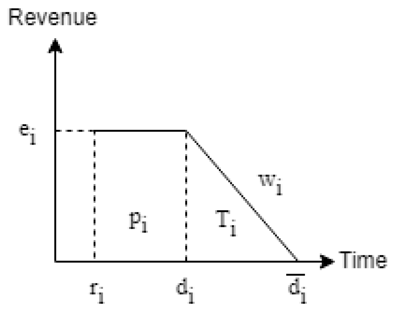
Numerous traditional scheduling problems assume a set of n orders to be accepted and scheduled in a specified production environment. An order i typically quotes a due date $d_i$ and a deadline $\overline{d_i}$. The due date is less than or equal to deadline. After an order i is completed at time $C_i$, the company receives a profit $e_i$ if $C_i$ is before $d_i$ and may get weighted penalties in the case of late delivery [1]. This profit calculation is depicted in Figure 1. A firm, nonetheless, must often choose the appropriate orders according to its available capacity, market focus, competitive advantage, or a combination of these [2]. This scheduling problem has transformed into an order acceptance and scheduling (OAS) problem involving the decision of accepting or rejecting orders and then scheduling the accepted orders on machines. Engels et al. [3] defined the OAS problem to be a combination of the knapsack and scheduling problems. The general objective is to maximize the total revenue $Q_i$ minus the tardiness penalties. Because OAS is a practical problem for enterprises in the supply chain, it has gained increasing research attention in recent decades [3,4,5,6,7,8].

OAS problems may involve a single machine [3,9,10], parallel machines [6,11,12,13], or a permutation flow shop [5,8,14]. To address these three machine types, some studies have proposed exact algorithms, such as the branch-and-bound algorithm [9], mixed integer programming [15], and dynamic programming [3,16]. Oğuz et al. [1] found some useful upper bound equations which reduce the computational effort in the branch-and-bound algorithm. However, if the number of job is larger than 15, branch-and-bound algorithm cannot solve them in 1 h. Nobibon and Leus [9] proposed the time-indexed formulations in a branch-and-bound algorithm with up to 50 jobs in a reasonable time.

For large-size and NP-hard problems [17], no algorithm can solve the problem in polynomial time. Many researchers have employed metaheuristic methods, such as genetic algorithms [2,18,19,20], tabu search [4], estimation of distribution algorithm (EDAs) [21], simulated annealing [15], and the artificial bee colony algorithm [8]. Cesaret et al. [4] proposed a tabu search algorithm, which was effective compared with m-ATCS and ISFAN based on the deviation from the UBs provided by MILP. The work of Wattanapornprom et al. [21] might be the first research to solve the OAS problem by EDAs. Their node based EDAs gain better results compared to GA with local search. In addition, Wattanapornprom et al. [21] found the consideration of OAS which increased the utilization rate in the supply chain. Finally, Slotnick [7] wrote an extensive review of the OAS problem, which is a good reference to understand the background.

Even though OAS problems have been studied extensively [7], prior OAS studied have not adopted the concept of green manufacturing that has received increasing attention among enterprises [22,23,24,25]. In particular, some recent works studied the carbon emission in the scheduling problems [26,27,28]. This paper focuses on the electricity power and excludes fuel consumption. Electricity power suppliers use gas-fired generation plants to supplement coal-fired generation plants during on-peak hours [29]. Because gas-fired generation plants usually emit less carbon per kilowatt hour of electricity produced than coal-fired generation plants, carbon emission during on-peak hours is lower than that during mid-peak and off-peak hours [30,31].

By contrast, the electricity cost during the on-peak hours is higher than that during mid-peak and off-peak hours if time-of-use electricity (TOU) tariff is used. The electricity cost of coal-fired generation plants is lower than that of gas-fired generation plants. There is an apparent trade-off between green scheduling and the electricity cost. To the best of our knowledge, although Zhang et al. [31] studied the trade-off for flowshop scheduling problems, no study on OAS has investigated sustainable scheduling, TOU costs, and a combination of both. The present study aims to solve the OAS problem and achieve carbon footprint reduction and minimization of electricity fees, which are the major contributions of this study.

To address the trade-off between carbon footprint reduction and TOU electricity costs, the carbon emission tax was introduced. In some countries, the carbon emission tax is defined per tonne (https://en.wikipedia.org/wiki/Carbon_tax). This study examined the carbon emission tax of selected countries, and they are listed in

Table 1. The CO₂ tax per ton in some selected countries.

Country	Price	Currency	USD (2019/5)
Japan	2400	Yen	21.852
Korea	31,828	KRW	27.0664
India	400	INR	5.7288
Denmark	13	Euro	14.5997
Ireland	20	Euro	22.4571
Netherlands	27	NLG	14.4
Sweden	930	SEK	96.39
Switzerland	36	CHF	35.49
Canada/Quebec	3.5	CDN	2.6

. For example, in Japan, the carbon emission tax per tonne is 2400 Yen (US$21.852 as of May 2019). Sweden charges the highest carbon emission tax. The average carbon emission tax per ton is $26.73155 (Table 1). Given the average carbon emission tax, the revenue of each accepted order is subtracted from the TOU electricity cost and carbon emission tax according to the power consumption of each order.

This paper proposes a new OAS problem considering the carbon emission cost and the TOU tariff. To solve this problem, a mathematical model of mixed-integer linear programming (MILP) was formulated and solved using IBM CPLEX 12.9. MILP normally requires a higher computational time to obtain an optimal solution. Prior studies investigated linear programming (LP) relaxation and applying less binary variables [32], preprocessing [33], objective scaling [34], Lagrangian Relaxation [12], MILP-based heuristics, an evolutionary algorithm within MILP [35,36], executing primal or the dual simplex method at the child nodes and different types of cuts [33,37], and so on. In this research, we use LP to obtain an initial solution which was input to the MILP model. This proposed method is MIPStart. We compared the performance of the original MILP model and that with an LP and MIPStart method.

The remainder of the paper is organized as follows. Section 2 shows the related works of order acceptance scheduling problems on a single machine. Section 3 presents the MILP formulations of the proposed problem. Section 3 presents LP relaxation and MIPStart method. Section 4 describes the LP relaxation and data generation procedures. Section 4 presents the experimental result obtained using the original MILP model and that with an initial solution. Section 5 concludes the paper and presents future research directions.

2. Literature Review

Regarding the OAS problem on a single machine, numerous works can be found. Stemming from Bartal et al. [16], Engels et al. [3] studied the objective function of minimizing the total weighted completion time and the penalty of the rejected jobs, ${\sum }_{i\in S}{w}_i{C}_i+{\sum }_{i\in \overline{S}}{e}_i$, instead of the makespan and sum of the penalty of the rejected orders, $C_{max}+{\sum }_{i\in \overline{S}}{e}_i$. This paper proves that the studied problem is weak NP-Complete. Most importantly, this is the first research that proposes the idea of a rejection machine. The rejected orders are sent to the rejection machine. That is, a single machine scheduling problem becomes a parallel machine scheduling problem. Due to this important characteristic, they demonstrate a dynamic programming algorithm that also yields a factor approximation algorithm (FPTAS). Because this paper does not conduct any experiments on the dynamic programming algorithm and the FPTAS, we do not know whether the two algorithms could solve the maximum jobs.

Rom and Slotnick [2] studied a genetic algorithm solving the OAS with tardiness penalties. The genetic algorithm employs the random key approach and determines the rejection orders when they evaluate the completion time of the orders. Additionally, some techniques are used to increase the population diversity, including clone removal, mutation, immigration, and changing the population size. Two local search operators are also used in the GAs. In their design-of-experiment (DOE), they suggested setting the population size to 200, randomly interchanging successive jobs when they perform the mutation, using the clone removal, and not applying immigration in the GAs. They compared a heuristic with the GAs. The results show the GAs outperform the myopic heuristic.

Oğus et al. [1] examined the release time, due day, deadlines, and the sequence-dependent setup times on a single machine. The objective function is to maximize the total revenue from a function of the total tardiness and deadline. They solved this problem by mixed-integer linear programming (MILP) in the small size problems up to 15 orders. Oğus et al. [1] also developed three heuristics to solve larger size problems up to 300 orders.

Unlike Engels et al. [3], when the single machine scheduling problem is transformed into a parallel machine scheduling problem, Tanaka [10] converted the sum of job completion cost into the general scheduling problem that modifies the job completion costs. The primary approach is to remove jobs i with the completion cost $f\left(\widehat{C_i^S}\right)$ being more than the revenue $Q_i$. Furthermore, the rejected jobs are moved to the end of the schedule. Tanaka [10] integrated this approach in the branch-and-bound algorithm for solving six sets with different objective functions of the single machine scheduling problems. Their experimental results show the significant efficiency when compared with the branch-and-bound algorithm in Nobibon and Leus [9]. In [10], 50 orders may take less than 1 s on average; however, Nobibon and Leus [9] required at least 24 s. We could see the significant difference of their branch-and-bound algorithm even though the latter considers some firm planned orders and the computer performance is not the same either. The only two conditions this method currently does not solve are when jobs are give deadlines and the idle times are forbidden.

Cesaret et al. [4] maximized total revenue on a single machine with sequence-dependent setup times and release date. The objective function is to maximize the total revenue, ${\sum }_{i\in S}(x_i{Q}_i-w_i{T}_i)$. A tabu search algorithm and two heuristics are compared on the instances up to 100 jobs. Because they supply the testing instances of 10, 15, 25, 50, and 100, this research adopts their instances to test our unified approach.

Chen et al. [38] proposed improved GAs with a local search for solving the single machine order acceptance problems. Later, Chen et al. [39] presented a new diversity metric to control population diversity. Both papers apply a same-site-copy-first principle [19] in their GAs. However, the performance improvement due to this operator is not reported when compared with other crossover operators. That is why we to apply the same-site-copy-first principle in our proposed crossover operator.

For a detailed review, Slotnick [7] wrote an excellent survey of the OAS problems. This paper points out five taxonomies of the related works. According to this review and the above referred articles, there is no research study on the time-of-tariff energy cost and CO₂ emission cost. Hence, the two new considerations are the significant contribution of this research.

3. Mathematical Formulations

Let n be a set of orders in the OAS problem for the three machine types. An order i has its own due date $d_i$, deadline $\overline{d_i}$, processing time $p_i$, and arrival time $r_i$. When order i is accepted and processed, if the completion time $C_i$ is before $d_i$, the company receives a revenue $e_i$. When tardiness occurs, $T_i$ must be equal to $max(0,C_i-d_i)$ and $C_i$ must be less than $\overline{d_i}$. If not, the order must be rejected without processing.

To model the formulations of the OAS problems, we employed the model provided by Oğuz et al. [1], as shown in Section 3.1. Then, we added constraints for calculating the carbon emission cost and electricity tariff (Section 3.2). In the model of Oğuz et al. [1], dummy order 0 and n+1 were added, denoted as $O_0$ and $O_{n+1}$. $O_0$ is the first position in the sequence, and $O_{n+1}$ occupies the last position. The two dummy orders are available at time zero. In addition, the processing time, due date, deadline, and revenue are also 0. ${\overline{d}}_{n+1}$ is set as the maximum due date among all the orders. We adopted the aforementioned settings proposed by Oğuz et al. [1]. We assumed that a factory works 24 h a day and the total manufacturing hours are no more than 24 h. Please access the variables used in MILP model in the abbreviation.

Finally, the time unit is the minutes for the arrival time, processing time, due day, and deadline. If an order arrives at 08:00, the value of $r_i$ is 240 min because the starting time is 0 at the midnight. The unit of profit, TOU cost and tax are in US dollars.

3.1. Basic Model of Order Acceptance Problem

Oğuz et al. [1] defined two decision variables. $a_i$ represents whether the order is accepted or not. $u_{ij}$ is the decision variable indicating whether order i is processed by order j.

$$a_i=\left\{\begin{array}{cc}1\hfill & \mathrm{When}\mathrm{order}i\mathrm{is}\mathrm{accepted}i\in O\hfill \\ 0\hfill & \mathrm{Otherwise}\hfill \end{array}\right.$$

$$u_{ij}=\left\{\begin{array}{cc}1\hfill & \mathrm{If}\mathrm{order}i\mathrm{is}\mathrm{processed}\mathrm{before}\mathrm{order}ji,j\in O,i\ne j\hfill \\ 0\hfill & \mathrm{Otherwise}\hfill \end{array}\right.$$

The following equations are the constraints for the OAS problems. A variable $R_i$ is used to evaluate the final profit of each order. The objective function in Equation (1) is used to maximize the total profit of each order.

$$\begin{array}{c}\hfill max\sum _{i=1}^n{R}_i\end{array}$$

(1)

S.T.

$$\begin{array}{cc}\hfill & {\sum }_{j=1,j\ne i}^{n+1}{u}_{ij}=a_i\forall i=0,\cdots ,n\end{array}$$

(2)

$$\begin{array}{cc}\hfill & {\sum }_{j=0,j\ne i}^n{u}_{ji}=a_i\forall i=1,\cdots ,n+1\end{array}$$

(3)

$$\begin{array}{cc}\hfill & C_i+(s_{ij}+p_j)u_{ij}+{\overline{d}}_i(u_{ij}-1)\le C_j\forall i=0,\cdots n,\forall j=1,\cdots n+1,i\ne j\end{array}$$

(4)

$$\begin{array}{cc}\hfill & (r_j+p_j)a_j+s_{ij}{u}_{ij}\le C_j\forall i=0,\cdots n,\forall j=1,\cdots n+1,i\ne j\end{array}$$

(5)

$$\begin{array}{cc}\hfill & C_i\le {\overline{d}}_i{a}_i\forall i=0,\cdots n+1\end{array}$$

(6)

$$\begin{array}{cc}\hfill & T_i\ge C_i-d_i\forall i=0,\cdots n+1\end{array}$$

(7)

$$\begin{array}{cc}\hfill & T_i\le ({\overline{d}}_i-d_i)a_i\forall i=0,\cdots n+1\end{array}$$

(8)

$$\begin{array}{cc}\hfill & T_i\ge 0\forall i=0,\cdots n+1\end{array}$$

(9)

$$\begin{array}{cc}\hfill & R_i\ge 0\forall i=1,\cdots n\end{array}$$

(10)

$$\begin{array}{cc}\hfill & C_0=0,C_{n+1}\le {max}_{i\in O}{\overline{d}}_i\end{array}$$

(11)

Equation (2) reveals that if order i is accepted, the order i precedes only one order, and Equation (3) shows that order i is preceded only by one order. If the order is rejected, it is not included in the sequence. Both constraints also forbid the preemption of orders. The constraint in Equation (4) indicates that, if order j is preceded by order i, order j has a greater completion time than order i; in addition, the sequence-dependent setup time $s_{ij}$ and processing time $p_j$ are higher. If order j is not preceded by order i, $C_j\ge$ 0 is the only constraint. The constraint in Equation (4) ensures this result, which prevents subtour in the sequence.

Equation (5) specifies that, if the order j is accepted and begins with sequence number i in the timetable, then the completion time of order j should be at least the sum of the release date, processing time, and sequence-dependent setup cost between orders i and j. If order i does not precede order j, the completion time of order j has a relaxed limit. The constraint in Equation (6) ensures that any orders completed after the due date are not accepted. If order j is not accepted, the limit is reduced to $C_j\ge$ 0. These constraints allow us to calculate the correct completion time of the order.

The constraints in Equations (7)–(9) define the tardiness for each order. Equations (11) and (12) set the completion time of dummy orders 0 and n+1, and the constraint in Equation (13) defines that both dummy orders are accepted.

$$\begin{array}{cc}\hfill & a_0=1,a_{n+1}=1\hfill \end{array}$$

(12)

$$\begin{array}{cc}\hfill & a_i\in \{0,1\},u_{ij}\in \{0,1\}\forall i=0,\cdots n,\forall j=1,\cdots n+1,i\ne j\hfill \end{array}$$

(13)

$$\begin{array}{cc}\hfill & C_{n+1}\ge \underset{i\in O}{min}{r}_i+\sum _{i\in O}(p_i{a}_i+\sum _{j\in O}{s}_{ji}{u}_{ji})\hfill \end{array}$$

(14)

$$\begin{array}{cc}\hfill & C_i\ge (r_i+p_i)a_i+\sum _{j\in O}{s}_{ji}{u}_{ji},\forall i=1,\cdots n\hfill \end{array}$$

(15)

Oğuz et al. [1] explored the possibility of using an effective inequality to improve the upper bound of LP relaxation in Equations (14) and (15). These inequalities ensure that the model does not break the variable $u_{ij}$ into too many small pieces and cause some orders to be rejected.

3.2. Mathematical Formulations for Considering the TOU Cost and Carbon Emission

Previous studies on OAS problems have considered that the completion time $C_i$ is associated with due day $d_i$. The present research studied the duration of each job in different TOU electricity hours and CO₂ emission intervals. To solve the problem more effectively, we introduce the starting time $S{T}_i$ of order i by considering TOU and CO₂ emission hours. Equation (16) can be used to calculate the starting time of order i based on its processing time, setup cost, and acceptance status $a_i$. The constraint in Equation (17) indicates that the starting time of job i must be greater than or equal to its arrival time. Equations (16) and (17) provide the correct calculation of $S{T}_i$.

$$\begin{array}{cc}\hfill & C_i-p_i{a}_i-\sum _{j=0}^n{s}_{ji}{u}_{ji}\ge S{T}_i\forall i\in O\forall i\ne j\hfill \end{array}$$

(16)

$$\begin{array}{cc}\hfill & r_i{a}_i\le S{T}_i\forall i\in O\hfill \end{array}$$

(17)

$$\begin{array}{cc}\hfill & \sum _{i=1}^{n+1}{x}_{ik}\le b_k-b_{k-1}\forall k=1,\cdots ,m\hfill \end{array}$$

(18)

$$\begin{array}{cc}\hfill & \sum _{k=1}^m{x}_{ik}\ge C_i-S{T}_i\forall i\in O\hfill \end{array}$$

(19)

$$\begin{array}{cc}\hfill & x_{ik}\ge min(C_i,a_i{b}_k)-max(S{T}_i,a_i{b}_{k-1})\forall i\in O\forall k=1,\cdots ,m\hfill \end{array}$$

(20)

$$\begin{array}{cc}\hfill & \sum _{i=1}^{n+1}{z}_{ik}\le q_k-q_{k-1}\forall k=1,\cdots ,h\hfill \end{array}$$

(21)

$$\begin{array}{cc}\hfill & \sum _{k=1}^h{z}_{i,k}\ge C_i-S{T}_i\forall i\in O\hfill \end{array}$$

(22)

$$\begin{array}{cc}\hfill & z_{ik}\ge min(C_i,a_i{q}_k)-max(S{T}_i,a_i{q}_{k-1})\forall i\in O\forall k=1,\cdots ,h\hfill \end{array}$$

(23)

$$\begin{array}{cc}\hfill & R_i\le a_i(e_i-T_i{w}_i)-\sum _{k=1}^m(\frac{x_{ik}}{60}\times E{C}_k\times {\Omega }_i)-\sum _{k=1}^h(\frac{z_{ik}}{60}\times tax\times q_k\times {\Omega }_i)\forall i\in O\hfill \end{array}$$

(24)

Using Equations (18)–(20), we calculate the $x_{ik}$ according to the time-of-use electricity hours. Equation (18) indicates that, when some jobs are allocated within the period $b_{k-1}$ to $b_k$, the total processing time cannot exceed the duration of this period. Equation (19) indicates that the total processing time of job i across different electricity hours must be greater than or equal to the completion time of the job minus the starting time. This equation keeps the integrity of the processing time of each job. Equation (20) indicates that, when the job cross-interval processing occurs, it is necessary to separately calculate the processing time in which the current interval is allocated and the processing time to be allocated in the span. The parameter $x_{i,k}$ during this process is defined by the time spent between $S{T}_i$ and $C_i$. If the job i starts and ends in the same interval, $x_{ik}$ is reduced to $C_i-S{T}_i$ in Equation (20). By using Equation (20), we assume that the processing time of each order would not exceed more than two TOU emission periods.

Similarly, we use Equations (21)–(23) to calculate the production time of job i in the carbon emission period k. For most cases, we use Equation (22) to calculate $z_{i,k}$ because only a few orders would span different time intervals. Equation (22) also keeps the integrity of $z_{i,k}$. If an order is processed across two intervals, Equation (23) can be used to calculate the first and second parts of the processing time. We also assume that the processing time of each order does not span more than two CO₂ emission periods.

In Equation (24), the first term provides the accepted order i minus the tardiness cost. The tardiness penalty is $w_i{T}_i$, where $w_i$ is the customer weight represented as a proportional lateness discount [2]. The second part of Equation (24) indicates the corresponding electricity bill generated by each accepted order according to the amount of time and power consumption during TOU periods. Finally, the last part is used to calculate the carbon emission cost of each order.

4. LP Relaxation and MIPStart Method

Although we can calculate an optimal solution in the proposed MILP optimization model, obtaining such solutions for large problems would be a time-consuming process. Relaxing the conditions for the integer decision variables $u_{ij}$ and $a_i$ might yield the upper-bound values in a short time. We can designate such a relaxed model as our LP model to represent the obtained results from this approach. Because $u_{ij}$ and $a_i$ are no longer integer values, the objective function values or upper-bound values might be higher than those derived in the MILP version. Specifically, our LP model may generate infeasible solutions. The reason is some $u_{ij}$ and $a_i$ are no longer 0, which increase the total revenue. However, the deadline of LP solution may not meet the real case.

In addition to our LP relaxation method, we propose another approach named MIPStart, which takes advantage of CPLEX. In this approach, the solution $u_{ij}$ obtained by LP relaxation is injected into the MILP as the starting solution. Because the value of $u_{ij}$ is a real number between 0 and 1, we convert the $u_{ij}$ into the integer value. If $u_{ij}$ is greater than or equal to 0.5, we set the $u_{ij}$ as 1. Otherwise, the revised $u_{ij}$ is 0. After this transformation, $u_{ij}$ is turned into the one-dimensional array required by CPLEX. CPLEX does not support an initial solution with two-dimensions.

When we inject the array, $a_i$ is obtained immediately. Because of the existence of infeasible solutions, we use an automatic model in CPLEX, which can convert an infeasible solution into a feasible solution. It is a built-in characteristic provided by CPLEX. We conducted evaluations to determine whether we could produce solutions of relatively high quality or reduce the computation time by using the mentioned models and approaches.

5. Testing Instances and Electricity Data

Cesaret et al. [4] supplied the testing OAS instances on a single machine. The order sizes are 10, 15, 25, 50, and 100. The problem comprises $\tau$ and R parameters of values 1, 3, 5, 7, and 9. Each problem combination has 10 instance replications. The total number of instances is 1250. The objective is to maximize the total revenue on a single machine with sequence-dependent setup times and release date. Because no study has investigated the TOU tariff for OAS problems, we generated the corresponding energy consumption requirements for the above instances. The power consumption (kW) of each order ${\Omega }_i$ is in the range $U(1,20)$. The generated instances are available at Github (https://github.com/worldstar/OpenGA/tree/master/instances/SingleMachineOASWithTOU). In our experiments, we selected $\tau$ and R with values 1, 5, and 9. In addition, the first instance replication was used because the MILP model takes a long time to yield results.

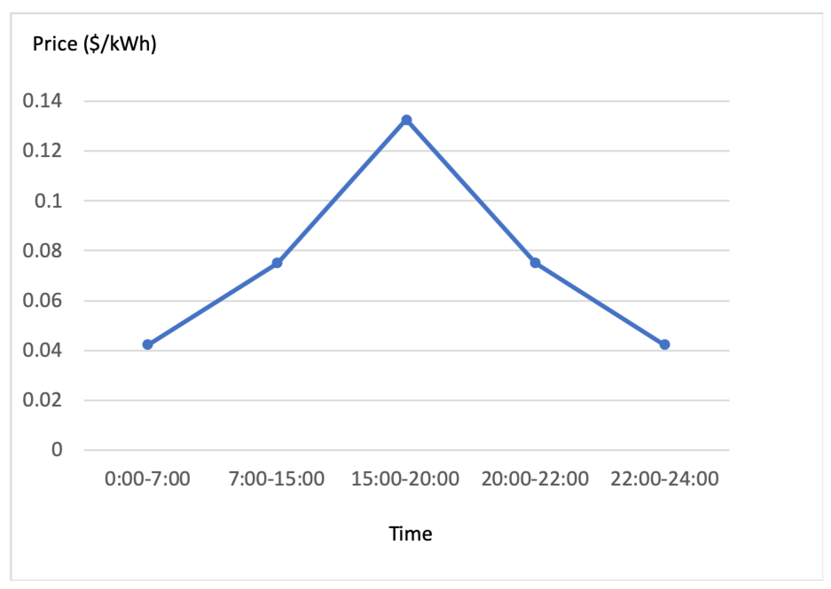
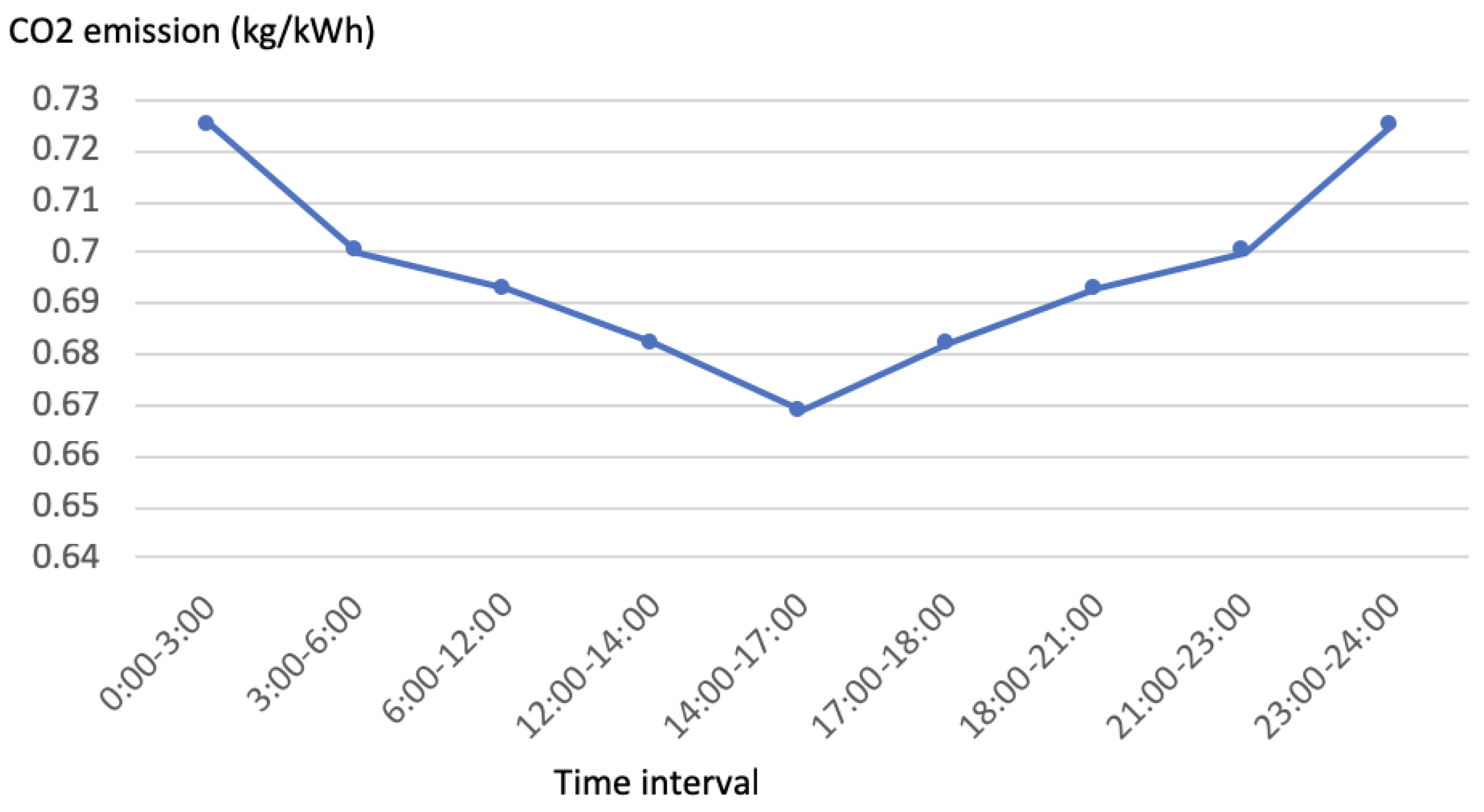
We calculated the TOU tariff and CO₂ emission cost by using data provided by Zhang et al. [31]. They provided the TOU tariff and CO₂ emissions in the summer season data shown in

Table 2. The time-of-use tariff in a summer day.

Time	Period	Price ($/kWh)
00:00–07:00	Off-peak	0.0422
07:00–15:00	Mid-peak	0.075
15:00–20:00	On-peak	0.1327
20:00–22:00	Mid-peak	0.075
22:00–24:00	Off-peak	0.0422

and

Table 3. The CO₂ emissions per kWh periods throughout 24 h.

Time Interval	CO2 Emission (kg/kWh)
00:00–03:00	0.725
03:00–06:00	0.7
06:00–12:00	0.693
12:00–14:00	0.682
14:00–17:00	0.669
17:00–18:00	0.682
18:00–21:00	0.693
21:00–23:00	0.7
23:00–24:00	0.725

, respectively. Figure 2 and Figure 3 represent the results of the two tables. A summer day contains five TOU periods from Monday to Saturday and nine CO₂ emission periods. The carbon dioxide emission factors ($q_k$) for electricity are from 0.682 to 0.725. It is quite similar to the one of Ireland. Liu et al. [40] adopted the average carbon dioxide emission factors for 1991–2006, which was 0.785 kgCO₂/kWh, while $q_i$ is 0.468 in the report for 2016 (https://www.seai.ie/resources/publications/Dublin-City-Baseline-Report.pdf). On Sunday, the off-peak is all day, hence, the electricity price does not influence the production sequence. Therefore, we only considered the TOU cost from Monday to Saturday.

The two tables clearly show that the carbon emission during the off-peak periods is higher than that during the on-peak period. We employed these electricity data to evaluate the objective function in Equation (24). In addition, based on the average carbon tax in Table 1, the average tax of carbon emission is $0.02673155 per kg.

6. Experiment Results

This section presents the results obtained by our proposed MILP mathematics model, LP relaxation model, and MIPStart method; these methods were run in IBM CPLEX 12.9 on an iMac 2017 with an Intel i5 3.4 GHz CPU and 16 GB of RAM. We applied the default setting of optimal gap value, which is 1e-06. Because problems with orders of magnitude larger than 25 are associated with high total computation times, each run of the program was limited to 1 h. Moreover, because we obtained the LP results before running any MIPStart experiments, we determined that the computation time of a problem with a 100-job order is 1 h instead of a few minutes. Hence, we set the computation time for both MILP and LP to 0.5 h when solving the 100-job instances.

In

Table 4. Comparison of the small orders.

Instances	UBMin	B				LP				MIPStart
		MILPUB	Obj	Gap	Time	LPUB	Obj	Gap	Time	MIPStartUB	Obj	Gap	Time
10-Tao1R1_1	118.719	118.719	118.707	0.01	0.9	122.627	122.627	3.29	0.0	118.719	118.707	0.01	0.8
10-Tao1R5_1	107.518	107.519	107.510	0.01	13.4	118.135	118.135	9.87	0.0	107.518	107.510	0.01	15.3
10-Tao1R9_1	93.627	93.629	93.619	0.01	3.2	93.646	93.646	0.02	0.0	93.627	93.619	0.01	3.6
10-Tao5R1_1	98.536	98.536	98.536	0.00	0.1	106.497	106.497	8.08	0.0	98.536	98.536	0.00	0.2
10-Tao5R5_1	98.626	98.632	98.623	0.00	0.6	105.641	105.641	7.11	0.0	98.626	98.623	0.00	0.6
10-Tao5R9_1	102.476	102.476	102.466	0.01	0.8	107.495	107.495	4.90	0.0	102.476	102.466	0.01	0.7
10-Tao9R1_1	57.697	57.697	57.697	0.00	0.0	94.688	94.688	64.11	0.0	57.697	57.697	0.00	0.0
10-Tao9R5_1	75.337	75.337	75.337	0.00	0.0	112.009	112.009	48.68	0.0	75.337	75.337	(0.00)	0.0
10-Tao9R9_1	106.506	106.506	106.506	0.00	0.1	137.544	137.544	29.14	0.0	106.506	106.506	0.00	0.1
15-Tao1R1_1	135.480	135.481	135.469	0.01	141.2	139.527	139.527	2.99	0.0	135.480	135.466	0.01	121.5
15-Tao1R5_1	212.594	212.602	212.582	0.01	3.7	218.160	218.157	2.62	0.1	212.594	212.582	0.01	3.4
15-Tao1R9_1	160.104	160.104	160.088	0.01	15.0	163.105	163.104	1.87	0.1	160.104	160.088	0.01	8.7
15-Tao5R1_1	147.337	147.337	147.322	0.01	160.7	157.799	157.799	7.10	0.1	147.337	147.322	0.01	158.1
15-Tao5R5_1	160.262	160.263	160.247	0.01	102.3	171.500	171.500	7.01	0.0	160.262	160.246	0.01	106.8
15-Tao5R9_1	135.759	135.759	135.746	0.01	27.1	143.246	143.243	5.51	0.1	135.759	135.746	0.01	30.2
15-Tao9R1_1	117.446	117.446	117.436	0.01	0.1	165.853	165.853	41.22	0.1	117.446	117.445	0.00	0.1
15-Tao9R5_1	138.584	138.584	138.584	0.00	0.1	182.657	182.657	31.80	0.0	138.584	138.584	0.00	0.2
15-Tao9R9_1	90.640	90.640	90.640	0.00	0.3	151.211	151.211	66.83	0.0	90.640	90.640	0.00	0.3

, the second column presents the minimum result of UB${}_{Min}$ obtained from MILP${}_{UB}$, LP${}_{UB}$, and MIPStart${}_{UB}$ for orders with 10, 15, and 20 jobs. UB${}_{Min}$ ensures that we have a tight upper-bound collection in the three methods. The abbreviation Obj represents the objective functions of the three algorithms within 1 h of CPU time. The percentage difference between the objective of each algorithm and UB${}_{Min}$ is presented in the Gap column. The gap of MILP can be calculated through Equation (25). Obj is the value of the objective function of the MILP model. Consider, for example, the instance 10-Tao1R1_1; the percentage difference between the objective value and the global upper bound UB${}_{Min}$ is 0.01%. All the small instances can be solved in 1 h, except for 20-Tao5R1_1 and 20-Tao5R9_1. This thus explains why the Gap of MILP is close to 0. Both 20-Tao5R1_1 and 20-Tao5R9_1 may need additional CPU time to obtain optimal solutions.

Because LP relaxation usually yields infeasible solutions, the objective value or upper-bound value is larger than UB${}_{Min}$. Hence, we can use Equation (26) to calculate the error ratio between the objective value of LP relaxation and UB${}_{Min}$. Of 27 instances, 15 have error ratios that are higher than 3%, despite the maximum CPU time being less than 0.2 s. The last four columns in the table present the results obtained for MIPStart; among 27 instances, 15 (e.g., 10-Tao1R1_1, 10-Tao1R9_1, and 10-Tao5R1_1) are associated with lower upper bounds than those provided by MILP. (The MILP${}_{UB}$ value observed for 10-Tao1R1_1 is larger than the MIPStart${}_{UB}$ value by 0.0001168.) The error ratio of MIPStart can also be derived using Equation (25).

$$\begin{array}{c}\hfill Gap=\frac{U{B}_{Min}-Obj}{U{B}_{Min}}\end{array}$$

(25)

$$\begin{array}{c}\hfill Ga{p}_{LP}=\frac{Ob{j}_{LP}-U{B}_{Min}}{U{B}_{Min}}\end{array}$$

(26)

Table 5. Comparison of the median to large-size orders.

Instances	UBMin	MILP				LP				MIPStart
		MILPUB	Obj	Gap	Time	LPUB	Obj	Gap	Time	MIPStartUB	Obj	Gap	Time
25-Tao1R1_1	308.001	308.001	301.016	2.27	3600.1	309.966	309.940	0.63	0.3	308.014	301.986	1.95	3600.8
25-Tao1R5_1	244.003	244.003	241.009	1.23	3601.2	244.007	244.006	0.00	0.2	244.003	241.013	1.23	3600.5
25-Tao1R9_1	286.120	286.120	280.100	2.10	3601.7	286.126	286.124	0.00	0.4	286.120	280.130	2.09	3605.9
25-Tao5R1_1	282.109	282.109	274.119	2.83	3600.2	285.873	285.872	1.33	0.2	282.110	260.254	7.75	3600.6
25-Tao5R5_1	263.781	263.905	242.698	7.99	3602.7	264.686	264.685	0.34	0.4	263.781	242.707	7.99	3601.2
25-Tao5R9_1	282.544	282.544	278.560	1.41	3600.2	298.088	298.072	5.50	0.3	285.553	277.510	1.78	3600.8
25-Tao9R1_1	207.053	207.058	207.053	0.00	1.9	264.676	264.676	27.83	0.3	207.053	207.053	0.00	1.9
25-Tao9R5_1	231.910	231.921	231.906	0.00	9.9	279.105	279.105	20.35	0.3	231.910	231.906	0.00	16.1
25-Tao9R9_1	262.167	262.168	262.142	0.01	22.4	294.743	294.741	12.42	0.3	262.167	262.142	0.01	62.2
50-Tao1R1_1	531.230	531.230	511.192	3.77	3600.1	532.380	532.339	0.21	6.0	531.230	510.045	3.99	3610.1
50-Tao1R5_1	591.570	591.570	573.514	3.05	3600.1	591.574	591.519	−0.01	10.1	591.570	548.438	7.29	3620.0
50-Tao1R9_1	555.901	555.901	535.844	3.61	3601.2	555.902	555.868	−0.01	6.2	555.902	540.640	2.75	3612.2
50-Tao5R1_1	524.979	524.979	480.088	8.55	3600.6	524.981	524.934	−0.01	5.0	524.979	499.832	4.79	3610.8
50-Tao5R5_1	581.880	581.884	553.080	4.95	3600.1	581.940	581.921	0.01	6.9	581.880	553.102	4.95	3609.1
50-Tao5R9_1	599.947	599.947	573.082	4.48	3600.1	599.989	599.985	0.01	3.3	599.950	567.067	5.48	3603.4
50-Tao9R1_1	416.004	416.004	380.781	8.47	3600.1	461.414	461.414	10.92	2.2	419.325	383.797	7.74	3602.2
50-Tao9R5_1	504.190	504.190	443.509	12.04	3600.1	535.789	535.788	6.27	2.3	507.442	441.458	12.44	3602.6
50-Tao9R9_1	542.467	542.954	492.117	9.28	3600.1	551.504	551.450	1.66	2.5	542.467	491.711	9.36	3602.6
100-Tao1R1_1	1075.388	1075.388	840.820	21.81	3601.0	1076.136	1070.835	−0.42	3600.5	1075.449	742.110	30.99	3601.0
100-Tao1R5_1	1163.011	1163.011	803.485	30.91	3601.5	1163.011	1162.542	−0.04	3600.7	1163.011	819.510	29.54	3601.5
100-Tao1R9_1	1158.153	1158.153	881.603	23.88	3601.2	1158.153	1157.813	−0.03	3600.8	1158.153	785.852	32.15	3601.2
100-Tao5R1_1	1222.156	1222.157	830.270	32.07	3600.3	1223.027	1222.905	0.06	3417.6	1222.156	818.226	33.05	3601.3
100-Tao5R5_1	1050.809	1050.809	660.690	37.13	3600.2	1051.055	1049.860	−0.09	3600.4	1050.809	501.685	52.26	3600.4
100-Tao5R9_1	1111.769	1111.769	509.713	54.15	3600.2	1111.809	1107.973	−0.34	3601.0	1111.769	362.242	67.42	3600.6
100-Tao9R1_1	1050.089	1050.089	983.831	6.31	3600.2	1057.981	1057.979	0.75	52.5	1050.311	950.074	9.52	1856.9
100-Tao9R5_1	963.598	964.714	841.833	12.64	3600.2	972.796	972.779	0.95	48.7	963.598	799.409	17.04	1849.0
100-Tao9R9_1	1024.393	1024.393	843.175	17.69	3600.2	1041.876	1041.777	1.70	79.4	1024.445	833.004	18.68	1880.6

presents the results of medium to large problems. Only four instances can be solved in 1 h. Our LP model can solve 25-job and 50-job problems in a few seconds; nevertheless, six orders require at least 1 h of computation time. Therefore, when solving the 100-job problem, we limited the CPU time for the LP and MILP optimization processes to 0.5 h for MIPStart. We observed that, for 16 instances, MILP provides a lower upper bound than that provided by MIPStart. For 11 instances, MIPStart provides superior upper bounds to those provided by MILP. As indicated in Table 4 and Table 5, the average error ratios derived for MILP, LP, and MIPStart are 5.97%, 9.59%, and 7.08%, respectively. The LP model has the highest error ratio among the three methods and generates some infeasible solutions; accordingly, LP optimization is not suitable for our studied problem. The MIPStart method has a higher error ratio (higher by 1.1%) than does the MILP optimization algorithm. The reason is that some infeasible solutions generated by LP are injected into MIPStart, and those injected solutions are not useful for pruning nodes in CPLEX 12.9. Hence, future research could employ some metaheuristic algorithms, such as genetic algorithms [2,18,20], Tabu search [4], and simulated annealing [15], to solve this new problem first and then inject the new solution into MILP.

7. Conclusions and Future Research

Even though OAS problem has been studied extensively [4,7,9,33], no previous research has studied the effects of the carbon footprint reduction and the TOU tariff. As a result, the major contribution of this paper is to solve the new OAS problem considering the two effects. Because a trade-off exists between carbon emission and electricity cost, a practical implication for electricity policy maker is that they cannot promote one direction alone. To calculate the CO₂ emission cost, a per-kilogram carbon tax was introduced so that the carbon emissions were transformed into the cost function. We extended the MILP formulations of Oğuz et al. [1] to solve this problem with CPLEX. If the conditions for two decision variables were relaxed, this MILP optimization would be converted into an LP model.

LP model usually solves a problem in a short time compared to MILP model. We further use LP relaxation to obtain an initial solution and then inject that initial solution into the MILP model, thus yielding a third method, namely MIPStart. When we compared the performance of the three methods, we determined that MILP is often significantly superior to LP because LP cannot feasibly solve many solutions. MIPStart would obtain few tighter upper bounds, which might be not useful to improve computational burden. Original structure of MILP is slightly superior to MIPStart in terms of the error ratio. The result is similar to the one of Alemany et al. [32]. We recommend that practitioners first use an algorithm to derive a feasible constructed solution in a short time and then adopt this constructed solution in MILP optimization.

For future research, we suggest that scholars employ some mathematical methods that could enhance the solution quality of the MILP model [9,41], including time-indexed formulations [9], preprocessing, cover cuts [33], and Lagrangian Relaxation [12]. Nobibon and Leus [9] employed time-indexed formulations, and solved problems with up to 50 jobs in a reasonable time. Other promising techniques include preprocessing and cover cuts in commercial solvers [33] and Lagrangian Relaxation [12]. Moreover, we could apply real-world requirements to simplify the proposed problem, which considers an OAS with carbon footprint reduction or with a TOU tariff separately. Metaheuristic algorithms, such as Tabu search [4], simulated annealing [15], and genetic algorithms [2,20], have also been proven effective for OAS problems. These algorithms are suitable for generating suitable initial solutions in a short time; such solutions can be injected into an MILP model. Deriving lower UBs and calculating an optimal solution in a reasonable time would be valuable.