Effects of Roadside Trees and Road Orientation on Thermal Environment in a Tropical City

Abstract

Emerging tropical cities are experiencing rapid population growth and development, which can greatly affect the thermal environments. The effects of roadside trees and road orientation on the outdoor thermal environment were investigated on four different roads in Kuala Lumpur, Malaysia. Field measurements were conducted to assess outdoor thermal environments, where the selection of sites was based on different roadside tree morphological features and road orientations. Outdoor air temperature (T_a), relative humidity (RH), globe temperature (T_g), wind speed (WS), and wind direction (WD) were measured. Absolute humidity (AH) was estimated based on relative humidity and air temperature. Planting dense canopy trees with an average sky view factor (SVF) of 0.07 reduced the mean radiant temperature (T_mrt) by 35% and the physiological equivalent temperature (PET) by 25%. East–West (E–W) and Northwest–Southeast (NW–SE) oriented roads had high PET values of 41 °C and 43 °C, respectively. North–South (N–S) and Northeast–Southwest (NE–SW) orientated roads had lower PET values (37 °C), providing improved outdoor microclimate. Roadside trees provided greater cooling potential in E–W and NW–SE oriented roads. The findings are useful for urban road design in tropical cities in order to improve the outdoor thermal environment and pedestrian comfort.

1. Introduction

Climate change has affected human health through heat-related illnesses, which will continue based on future predictions [1,2]. This includes an increase in the frequency and intensity of heat waves and thermal stress, which can result in an increase in human mortality rates [1]. For example, in August 2003, France experienced a heat wave event that caused approximately 14,800 heat-related deaths [3]. Heat stress mortality has been shown to increase in urban or developing areas [4]. In addition to climate change, outdoor air temperatures in urban areas have increased significantly due to rapid development and contribution from anthropogenic heat, such as heat release from automobiles, air conditioning, and industrial facilities. These factors have resulted in urban areas having higher temperatures than their rural counterparts, known as the urban heat island (UHI) phenomenon [5,6]. UHI is the most significant thermal environmental modification caused by urbanization [7] and is a major future factor in heat-stress-related mortality. Therefore, in order to mitigate further events that could negatively affect human health, urban environments need to be modified [8]. To this end, the UHI effect and the outdoor thermal environment have been studied extensively worldwide [9,10,11,12].

The outdoor thermal environment is governed by microclimate parameters, which have more diverse and complex interactions compared to an indoor environment [13]. Hence, improving the outdoor thermal environment can reduce heat-related illness and mortality while elevating the comfort level of pedestrians. These changes can also benefit the physical, environmental, economic, and social aspects of a city [14,15]. Studies of outdoor thermal environments have been conducted in both temperate [16,17,18,19] and tropical regions [20,21,22,23], where trees and urban green areas are popular solutions for mitigating the UHI effect [24,25,26]. Urban vegetation provides shelter and shade, while lowering the temperature of the urban areas [7,27,28,29]. However, the value and potential role of roadside trees in mitigating UHI effects are often underestimated [30,31]. Moreover, planting roadside trees in limited and constrained spaces is expected to result in poor drainage, root drowning, insufficient soil, and lack of growth space [32,33,34].

In the capital city of Malaysia, Kuala Lumpur, it has been proposed that the thermal environment of the city’s urban areas could be improved by planting roadside trees. While research regarding the mitigating effects of urban greenery has taken place, and guidelines for improving the outdoor thermal environment have been published, most of these studies were conducted in temperate climates. These studies hypothesized that the findings could not be easily adopted in tropical countries like Malaysia due to distinct climate differences, including higher outdoor temperatures and humidity. Changes in the solar angle in tropical regions are also small compared to regions of higher latitudes. Therefore, the main objectives of this study were to (1) investigate the effects of different roadside tree configurations and road orientations on the outdoor thermal environment and (2) evaluate the outdoor thermal comfort under such conditions in a tropical city by means of field measurements.

2. Materials and Methods

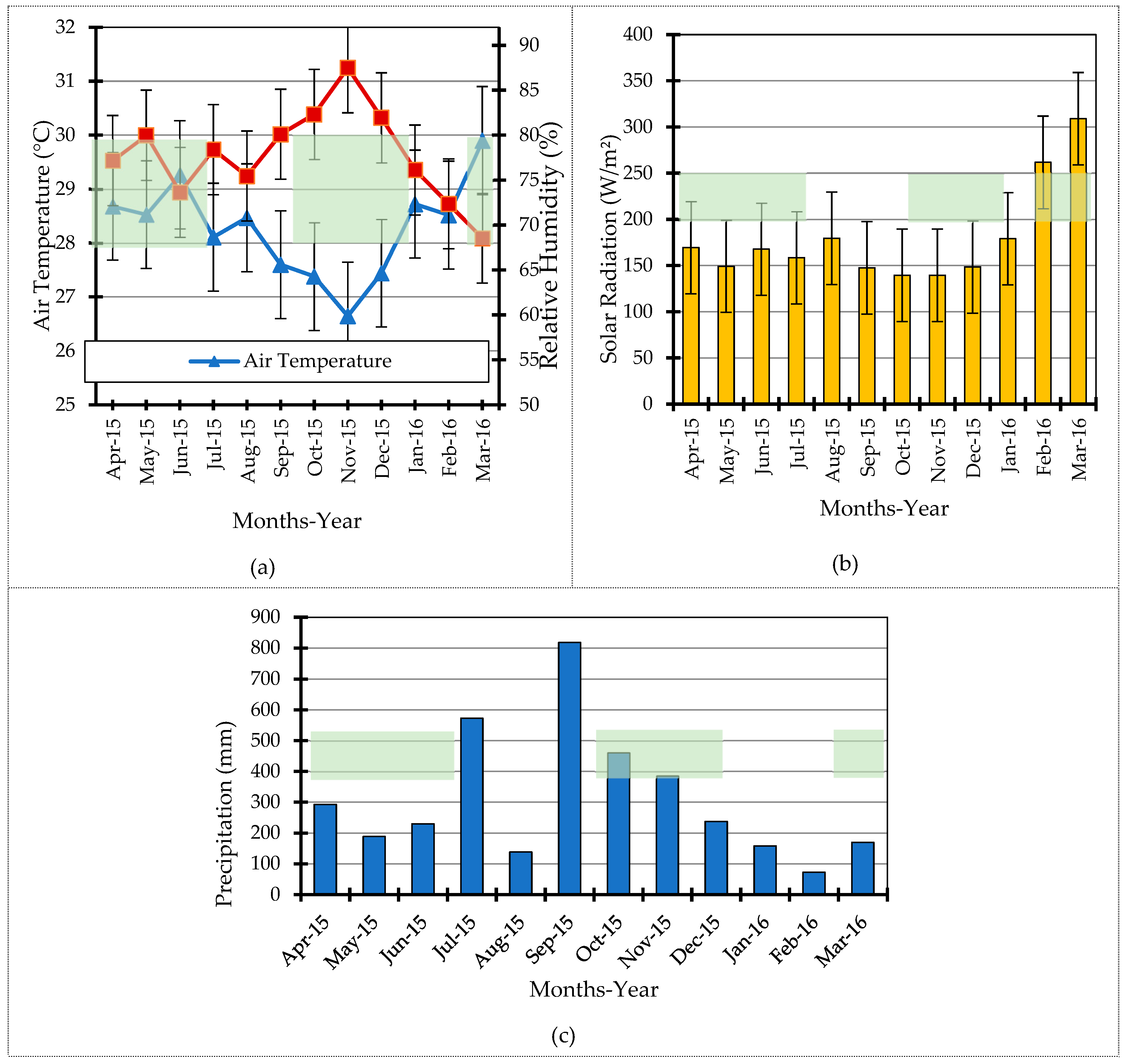
2.1. Climatic Conditions

Malaysia is located between 1° and 7° North (latitude) and 100° and 120° East (longitude), near the equator in Southeast Asia on the South China Sea. The climate is classified as tropical rainforest, (Af), based on the Köppen-Geiger climate classification [35] with no distinct seasonal variation.

Figure 1 shows the variation in outdoor climate conditions from April 2015 to March 2016, which is within the period of field measurement, as measured at a weather station mounted on the rooftop of the Malaysia-Japan International Institute of Technology (MJIIT) building. The average outdoor temperature is relatively constant throughout the year (27–30 °C). The humidity is generally high (~78% average relative humidity), with a total annual precipitation of 3727 mm, and the average monthly solar radiation is 139–309 W/m².

As the field-measurements were conducted during different months. The solar radiation at each measurement site began to increase at 07:00, continued to rise steadily, peaked from 11:00–13:00, and then began to descend until 19:00. The outdoor air temperatures showed a similar pattern to the diurnal cycle of the solar radiation as shown in Figure 2.

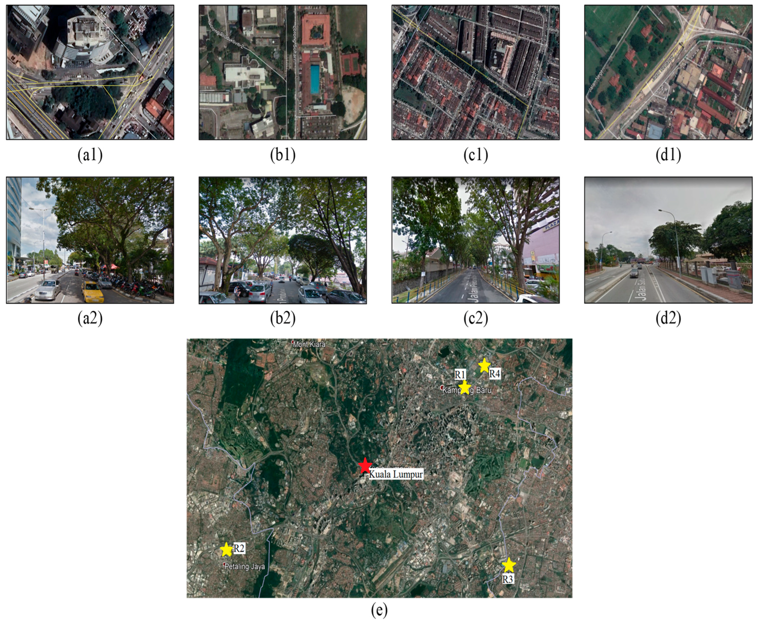
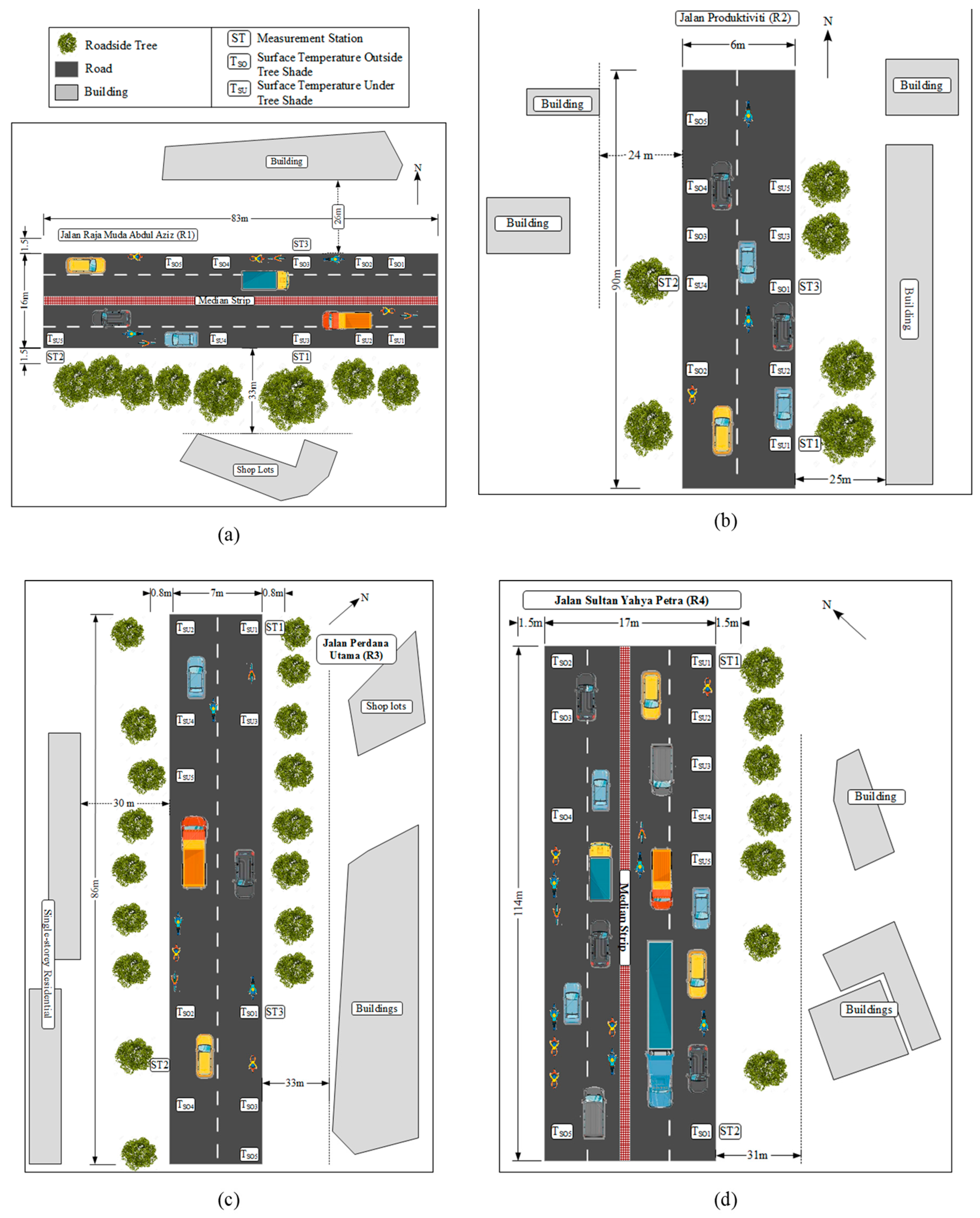
2.2. Measurement Sites and Periods

Selection of the urban roads for this study was based on roadside tree canopy coverage and tree height. In addition, different road orientations were selected, including the main orientations of East–West (E–W) and North–South (N–S) and intermediate orientations of Northwest–Southeast (NW–SE) and Northeast–Southwest (NE–SW), in order to incorporate the most common orientations. Four roads were chosen as measurement locations—Jalan Raja Muda Abdul Aziz (R1) (E–W), Jalan Produktiviti (R2) (N–S), Jalan Perdana Utama (R3) (NW–SE), and Jalan Sultan Yahya Petra (R4) (NE–SW). All roads within this study are situated within a 7 km radius of Kuala Lumpur city centre (Figure 3). The road segment length ranged from 83.0 m to 113.6 m, while the road width ranged from 6.2 to 16.6 m. The trees were located at both sides of the road for R2 and R3. In contrast, trees at R1 and R4 were only on one side which approximately 0.5–1.2 m distance.

All streets contained two tree species, Narra (Pterocarpus indicus; a broad-leafed deciduous tree) and Monkey pod tree (Samanea saman; a wide-canopied tree with a large symmetrical umbrella-shaped crown) (Figure 4). The location of roadside trees were randomly selected within close proximity of the urban city center of Kuala Lumpur. This was due to the difficulty of finding an ideal location for real measurement of an emerging tropical country.

As the focus of this study was on the urban roads with roadside trees, all selected road segments were located approximately 24.9–33.1 m from surrounding buildings to ensure that they were not shading the roads. This ensured that the data collected was not affected by any other factors, apart from the roadside trees. The tallest building (~46 m) was located at R1, while the lowest was situated at R2 (4 m). Field measurements were conducted to collect data from each site for two selected clear sunny days between April 2015 and March 2016. Field measurements for R1 and R2 were conducted between April 2015 and June 2015, while for R3 and R4, field measurements were conducted between October 2015 and November 2015. One extra field measurement was conducted for R3 in March 2016 to substitute the for the field measurement conducted on October 2015 due to incomplete data. Although the measurement of each road was conducted with a large time gap between April, June, October, and November, and measurement took two days for each location. The time disparities did not lead to uncertainties in weather conditions because of the consistent hot and humid climate experienced throughout the year. The mean annual outdoor air temperature and relative humidity (RH) were reported as 28 ± 2 °C and 80 ± 7%, respectively [36]. The measurement periods are limited to 09:30–13:30, 07:30–09:30, and 16:00–18:00 based on different locations that will be further describe in Section 2.3.

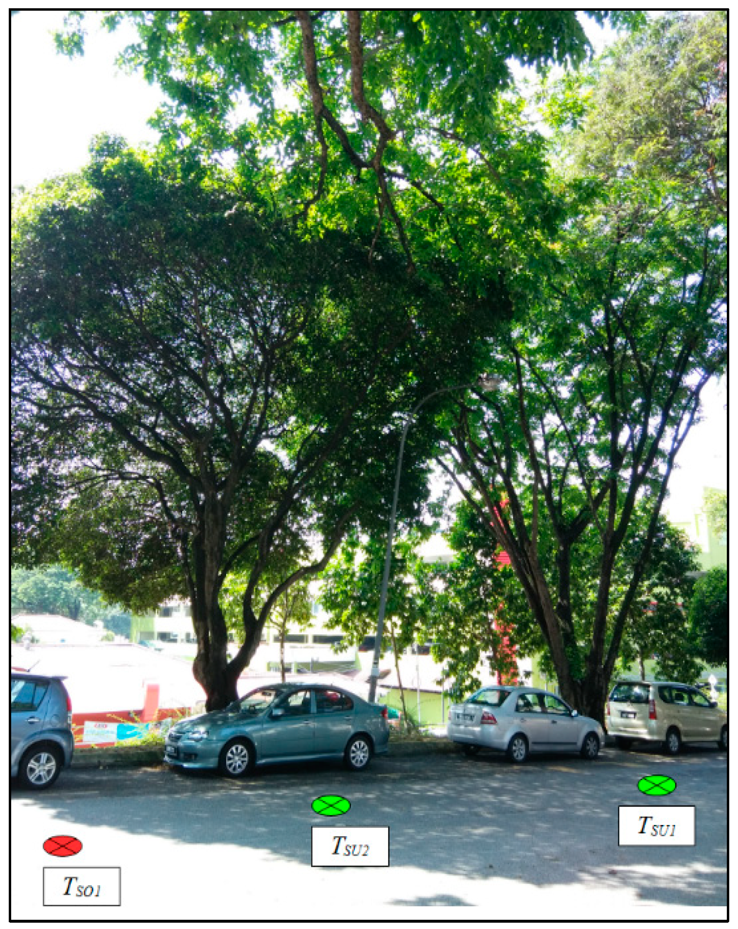
2.3. Microclimate Measurements

Five outdoor microclimate parameters were measured during each field study to assess outdoor thermal comfort: outdoor air temperature (T_a), relative humidity (RH), globe temperature (T_g), wind speed (WS), and wind direction (WD). Three measurement stations were placed along each selected road to capture the various values of tree canopy coverage. The first station (ST1) had all of the aforementioned measurement sensors, where one setup measured WS and WD, and a second setup consisted of T_a, RH, and T_g sensors. Due to limited instruments, the second (ST2) and third (ST3) stations only had T_a, RH, and T_g sensors. As there was only one station measuring WS and WD, these data could not be compared for different configurations of roadside trees along the same road. However, these factors were used as one of the main inputs to estimate the mean radiant temperature (T_mrt) and physiological equivalent temperature (PET). All instruments were placed 1.5 m above ground level [37] and were left for 30 min prior to data collection to equilibrate with local conditions. T_a and RH were measured by thermistor thermometer and capacitive hygrometer sensor respectively, and both sensors were mounted in the same data logger (Hobo U12 by Onset Computer Corporation, Bourne, United States of America (USA)) and covered in solar radiation shield to prevent the exposure to direct solar radiation and data interference. T_g was measured by a thermistor thermometer sensor (T&D TR-52i by T&D Corporation, Japan), with the external sensor sealed in a black celluloid globe of 40 mm diameter. The two-axis (2-D) ultrasonic anemometer (R.M. Young 86000 by R. M. Young Company, Michigan, USA) measured WS and WD, and both shared the same data logger (Campbell CR800 by Campbell Scientific Inc., Logan, USA). All sensors logged data automatically every minute and were placed 1.0 m away from the sidewalk curb. The focus of the field measurements was to analyze daytime microclimate variations to reveal the thermal benefits of roadside trees when their cooling effects were at the maximum level in the presence of high-intensity solar radiation [28,29,38,39,40]. For this study, the peak hours were between 11:00 and 13:00 [19], and therefore, measurements were taken for R1, R2, and R3 were taken between 09:30 and 13:30. The measurements at R4 were divided into early morning (07:30–09:30) and evening (16:00–18:00) sessions to investigate the effect of roadside trees on outdoor microclimate conditions for both early morning and evening hours.

In addition to the continuous measurements, periodic measurements of the road surface temperature (T_s) were made every four hours using an infrared thermal camera (InfRec Thermo Gear G100EX by Nippon Avionics Co., Ltd., Tokyo, Japan). Ten selected measurement locations were measured five times per day (approximately 08:00, 11:00, 14:00, and 17:00) for each selected road. The surface temperature measurements were conducted under (T_su) and outside (T_so) areas of tree shade (Figure 5). The stations and spots measurement locations for surface temperature are shown in Figure 6.

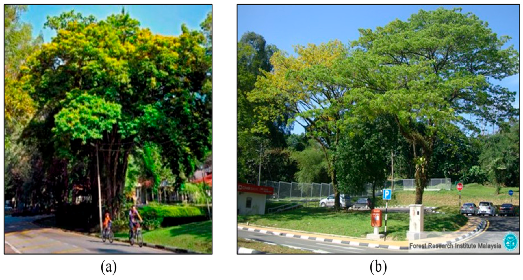
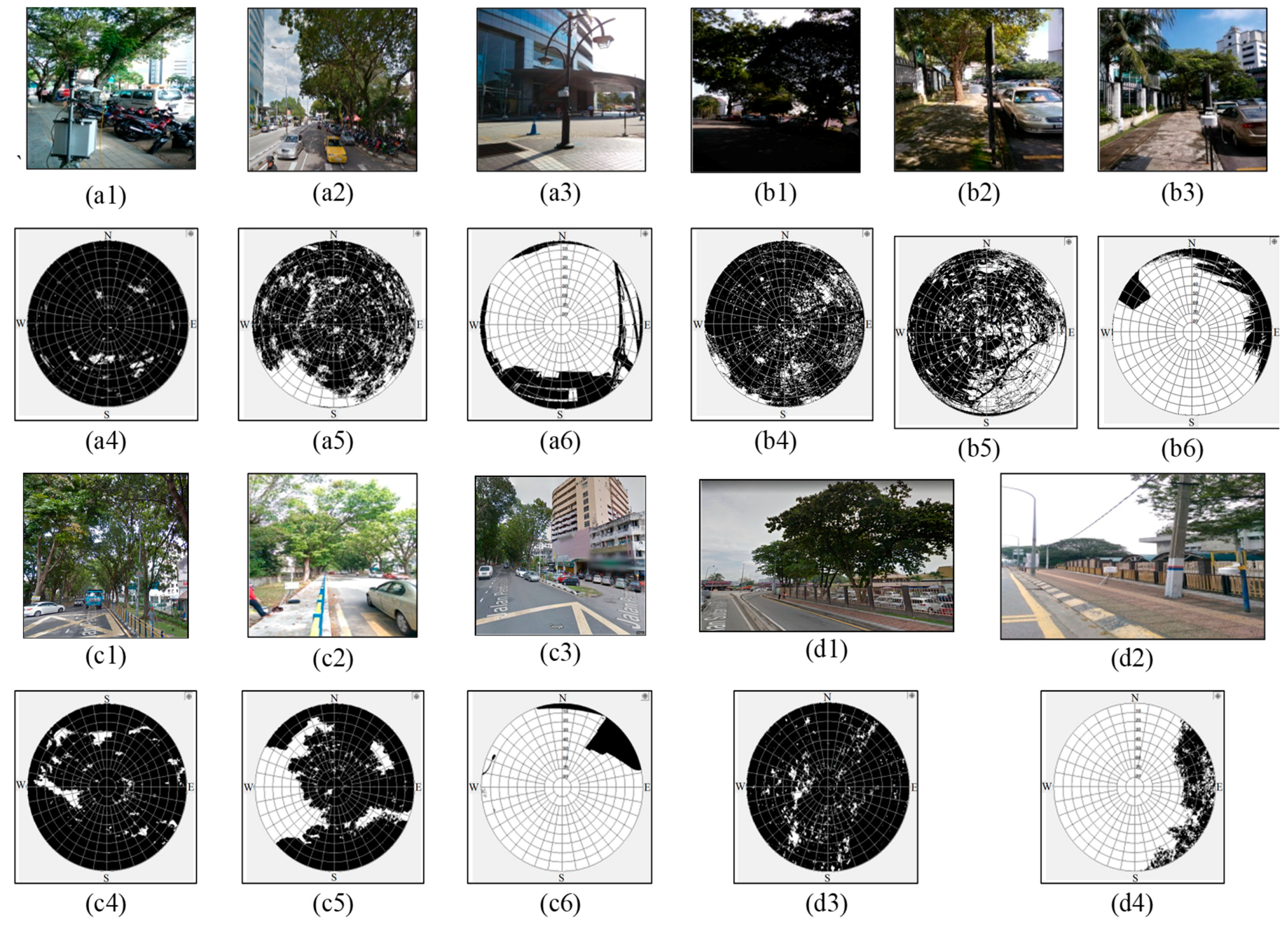
2.4. Measurement of Tree Canopy Coverage and Tree Height

The tree canopy coverage at the measurement locations was represented by the sky view factor (SVF), which was obtained using a digital single-lens reflex camera (DSLR, Canon COS 1200D by Canon Inc., Tokyo, Japan) equipped with a fisheye lens (Meike 6.5 mm F/2.0 by Hong Kong Meike Digital Technology Co., Ltd, Hong Kong, China). This enabled hemispherical or fisheye photos to be taken at all monitoring stations (ST1, ST2, and ST3) for each selected location of roadside trees. All SVF measurements were performed on the same day as the accompanying field survey. The photos were imported into RayMan software (version 1.2, Freiburg, Germany) to calculate the SVF [41]. Here, the roads were divided into three categories depending on the SVF: low SVF (R-LS) (SVF < 0.10) represents dense tree canopy; medium SVF (R-MS) (0.10 ≤ SVF < 0.79) represents sparse tree canopy; and high SVF (R-HS) (SVF ≥ 0.80). The SVF represents tree canopy coverage, except for a reference location with minor sky view obstruction by trees and other anthropogenic features, such as buildings and lampposts. The sky view obstruction was based on tree-canopy elements only (e.g., branches, leaves, and twigs). Therefore, to investigate the effects of different tree canopy densities on the thermal environment, R-HS with low sky obstruction (SVF ≥ 0.80) was chosen as a reference location for comparison with R-LS and R-MS (with tree canopies). Unless measurements were taken in the middle of a road, or in a location at a great distance from the site, it was very difficult to find a reference location where SVF = 1. The SVF measurement locations are denoted throughout the study as R1-LS (low SVF on R1), and every SVF level was available for all roads, except for R4 where only R4-LS and R4-HS were selected for measurements due to a lack of suitable R-MS tree canopy. The average SVF values for R-LS, R-MS, and R-HS are 0.07, 0.31, 0.86, respectively (Figure 7).

Tree height (H_T) was also investigated as a factor to fully consider the shading effects on the road thermal environment. The H_T values were measured using a laser range finder (TruPulse 200L by Laser Technology Inc., Colorado, USA) on the same day as the field survey. The total H_T was obtained from the sum of the crown thinness and height of the tree trunk, and varied from 6 to 21 m. The trees were categorized into the following four groups: short (6 to 9 m), medium (10 to 13 m), tall (14 to 17 m), and very tall (18 to 21 m) (

Table 1. Categories of roadside trees based on tree height.

Crown Thickness (m)	Number of Trees	Trunk Height (m)	Number of Trees	Total Tree Height (m)	Category	Number of Trees
4–5	3	2–3	1	6–9	Short	2
6–7	9	4–5	8	10–13	Medium	9
8–9	5	6–7	8	14–17	Tall	7
10–11	3	8–10	3	18–21	Very Tall	2

).

2.5. Estimation of Mean Radiant Temperature

T_mrt values were estimated considering the effects of convection and conduction on the black globe. The globe temperature is the weighted average of radiant and ambient temperatures. Since T_a, T_g, and WS are known, T_mrt was estimated based on Equation (1) [42]:

$$T_{mrt}={[{\left(T_g+273.15\right)}^4+\frac{h_{cg}}{\epsilon D_g^{0.4}}\left(T_g-T_a\right)]}^{\frac{1}{4}}-273.15,$$

(1)

where h_cg is the mean convective coefficient (1.10 × 10⁸WS^0.6), D_g is the globe diameter (m), and ɛ is emissivity (0.95).

2.6. Thermal Comfort Index

The PET was chosen as the thermal comfort index in this study and was calculated using RayMan software (version 1.2), which is suitable for the calculation of the radiation fluxes and thermal indices such as PET in both simple and complex environments. The software includes the Munich energy balance model for individuals (MEMI) and the calculation procedure for PET [39,43]. The required microclimate inputs were T_a, RH, WS, and T_mrt.

The PET classification ranges defined by Matzarakis and Mayer [44] were used as a reference to assess the outdoor thermal comfort and heat stress categories of urban spaces in Malaysia, as this reference is actually applicable for temperate regions. These PET ranges were also used in a similar study investigating thermal comfort of shaded outdoor spaces on a university campus in Malaysia [35].

3. Results

3.1. Relationship between Roadside Tree Configuration and Outdoor Thermal Environment

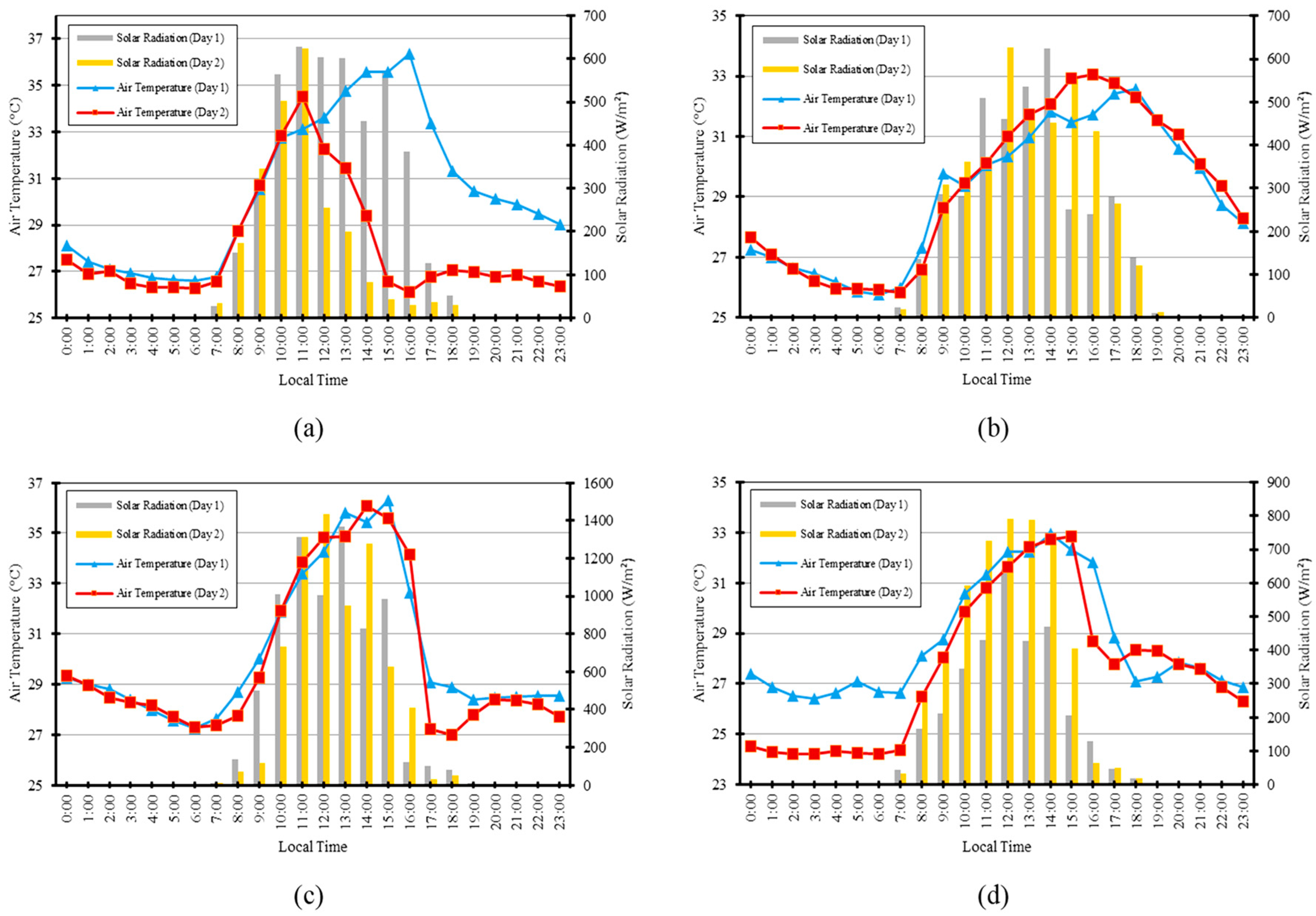
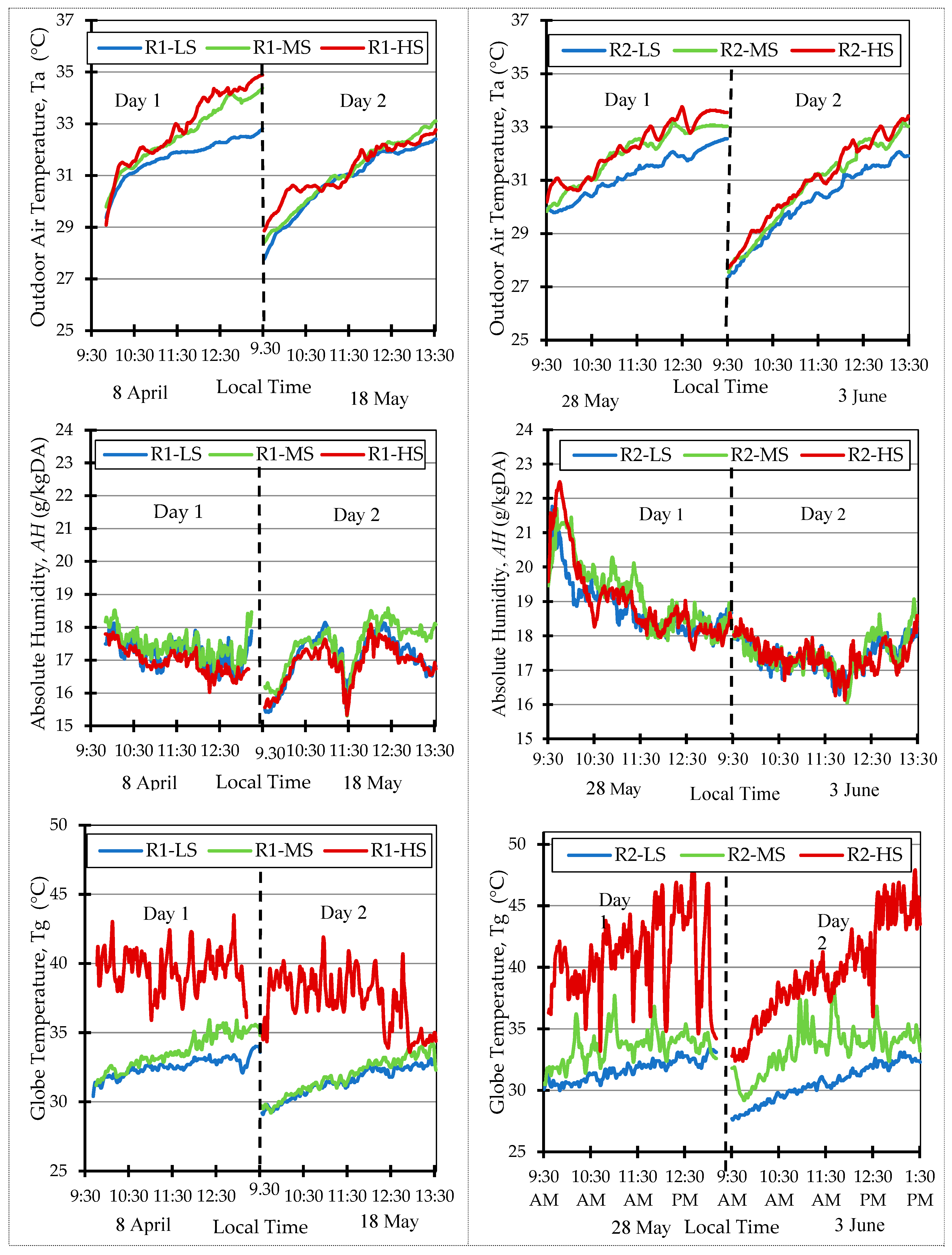
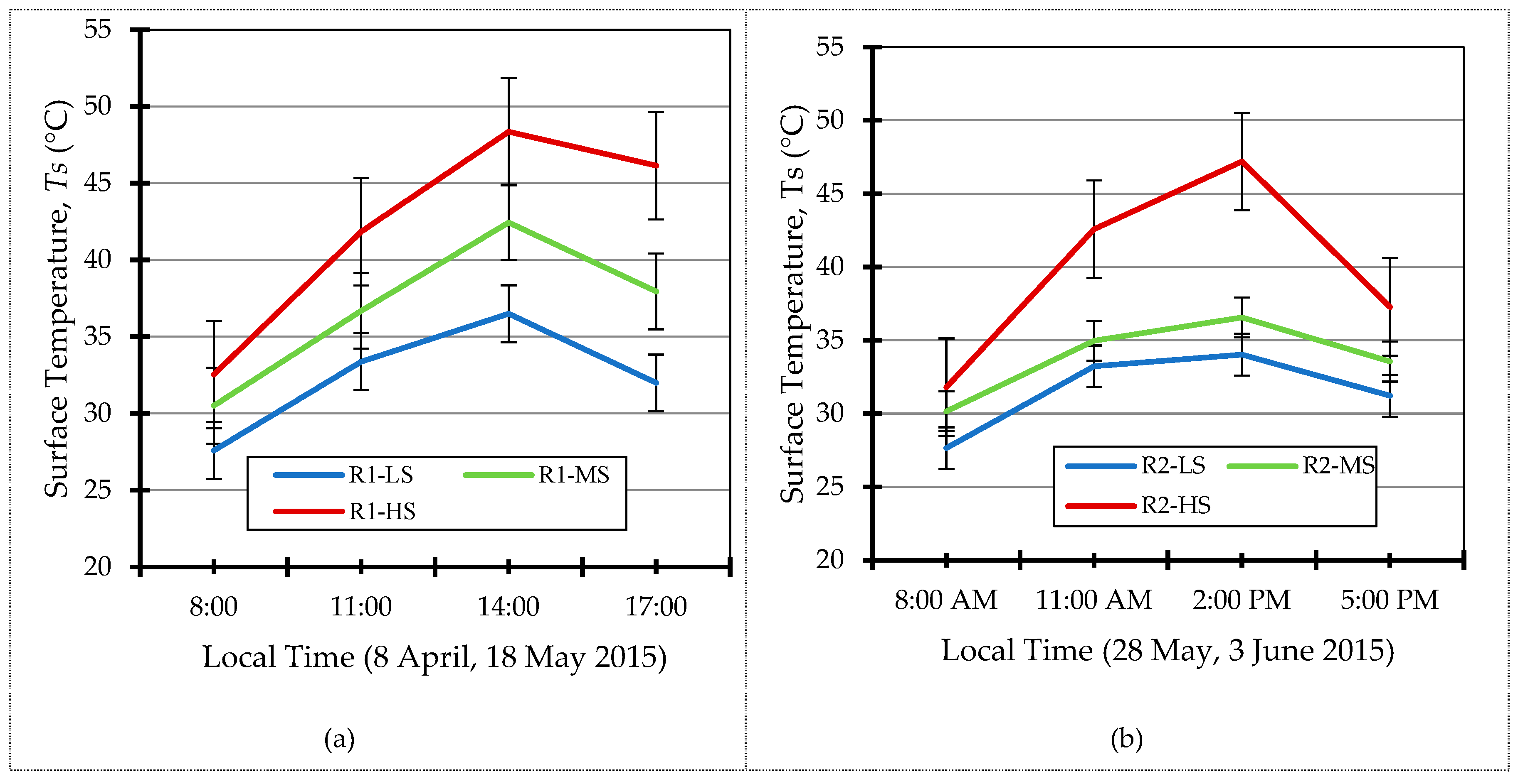
3.1.1. Variation in Outdoor Microclimate Parameters

The microclimate data for the two different measurement days for regions of different tree canopy densities (R-LS and R-MS) were compared to the reference location (R-HS). The roadside tree canopy coverage at R1 affected T_a and AH (Figure 8a). From 09:30 to 13:30, T_a gradually increased while AH decreased over time. The T_a values did not vary significantly for different roadside tree conditions, where a maximum T_a difference between R1-LS and R1-HS of 2.1 °C was observed (8 April at 13:30) (Figure 8a). Similarly, the difference in AH values between different tree canopy densities was small (<9%) (Figure 8a). Conversely, T_g showed a large dependence on tree canopy coverage. For R1-LS and R1-MS, T_g values were much lower than measured at R1-HS, with a maximum difference of 11.3 °C (Figure 8a). It was also observed that T_g was higher than T_a for all tree canopy densities.

At R2 (Figure 8b), T_a steadily increased, while AH decreased over time. Similar to results for R1, the differences in T_a and AH between R2-LS, R2-MS, and R2-HS were small, with maximum variations of 1.8 °C and 6%, respectively (Figure 8b). However, variations in T_g were large, with a maximum difference of 15.3 °C recorded on 28 May. The microclimate variation at R3 is shown in Figure 9a. T_a and AH showed similar trends as other roads. However, the differences in T_a and AH were noticeably larger, 4.3 °C and 16%, respectively. This may be due to the high number of roadside trees on both sides of R3, which reduced the wind speed, and increased differences in AH between locations with trees and the reference location. Furthermore, because surrounding buildings were blocked off, this may have influenced changes in wind effect, as well as changes due to the traffic flow of vehicles, and thus may not be due to the absolute effect from the high number of roadside trees. Wind is a very dynamic microclimatic parameter, and the value is always changing. Among all selected roads in this study, R3 contained the greatest number of trees and large difference in T_g, with a maximum of 14.1 °C on 19 March (11:06) (Figure 9a).

Figure 9b shows the variations in T_a, AH and T_g at R4. On day 1, the maximum T_a recorded at R4-HS was 32.4 °C, while under the same spatial and temporal conditions, the maximum T_a on day 2 was 34.8 °C. Both T_a and T_g found higher than T_a. The T_s for the R-LS, R-MS, and R-HS locations were compared to assess the effect of tree canopy coverage on T_s. The results show the effect of tree canopy coverage on T_s (Figure 8 and Figure 9). For all roads, T_s values under the tree canopy were always lower than those outside tree-shaded areas or at the reference location at any given time. The temperature difference between different SVF conditions was minimal during the early morning. The maximum difference in temperature (indicating the cooling effect of the trees) occurred at 2:00 pm for all roads. In summary, denser tree canopies resulted in lower T_s values, implying that roadside tree density affects T_s.

The following implications have been concluded. Firstly, the fluctuation of T_a was small, with a similar trend and difference of < 7% across all road conditions (R1‒R4). Higher AH values were measured for R-LS and R-MS sites compared to R-HS ones, likely due to the effect of tree transpiration (release of water vapor into the atmosphere). Comparison of the T_g values indicated that the cooling effect of roadside trees during the daytime was mainly due to a decrease in radiation flux due to the shade provided by the trees. Although an effect of wind reduction on the globe thermometer was observed, radiation effects were dominant. Several studies noted the insignificance of air temperature differences when comparing measurements under tree canopies with reference locations [17,45,46]. The findings of Narita et al. [17] demonstrated that the difference in air temperature was negligible throughout the day when compared to a parallel street without tree crowns. However, there was a clear shielding effect for solar radiation and downward long wave radiation, resulting in a lower road surface temperature. This implies that the main reason pedestrians feel thermally comfortable under tree crowns was not due to lower T_a values but where instead due to radiation effects. Our results indicate that the density of roadside trees affected T_g, which in turn affected the outdoor thermal environment.

3.1.2. Relationship between Roadside Tree Height and Road Surface Temperature

Figure 10 shows the average reduction in T_s with respect to tree height, where larger changes in T_s were observed with increasing tree height. Tall trees provided better shade quality than short trees by preventing solar exposure, resulting in lower T_s values. Loyde et al. [47] stated that large trees provide maximum shade coverage due to their height. Additional research also reported that the species and height of the tree affect the density of the shade, which consequently influences the road surface temperature [35,48,49]. In summary, our results showed that tall roadside trees (18–21 m) reduced T_s, more effectively by an average of 5.4 °C, corresponding to a 14% reduction compared to the unshaded T_s values.

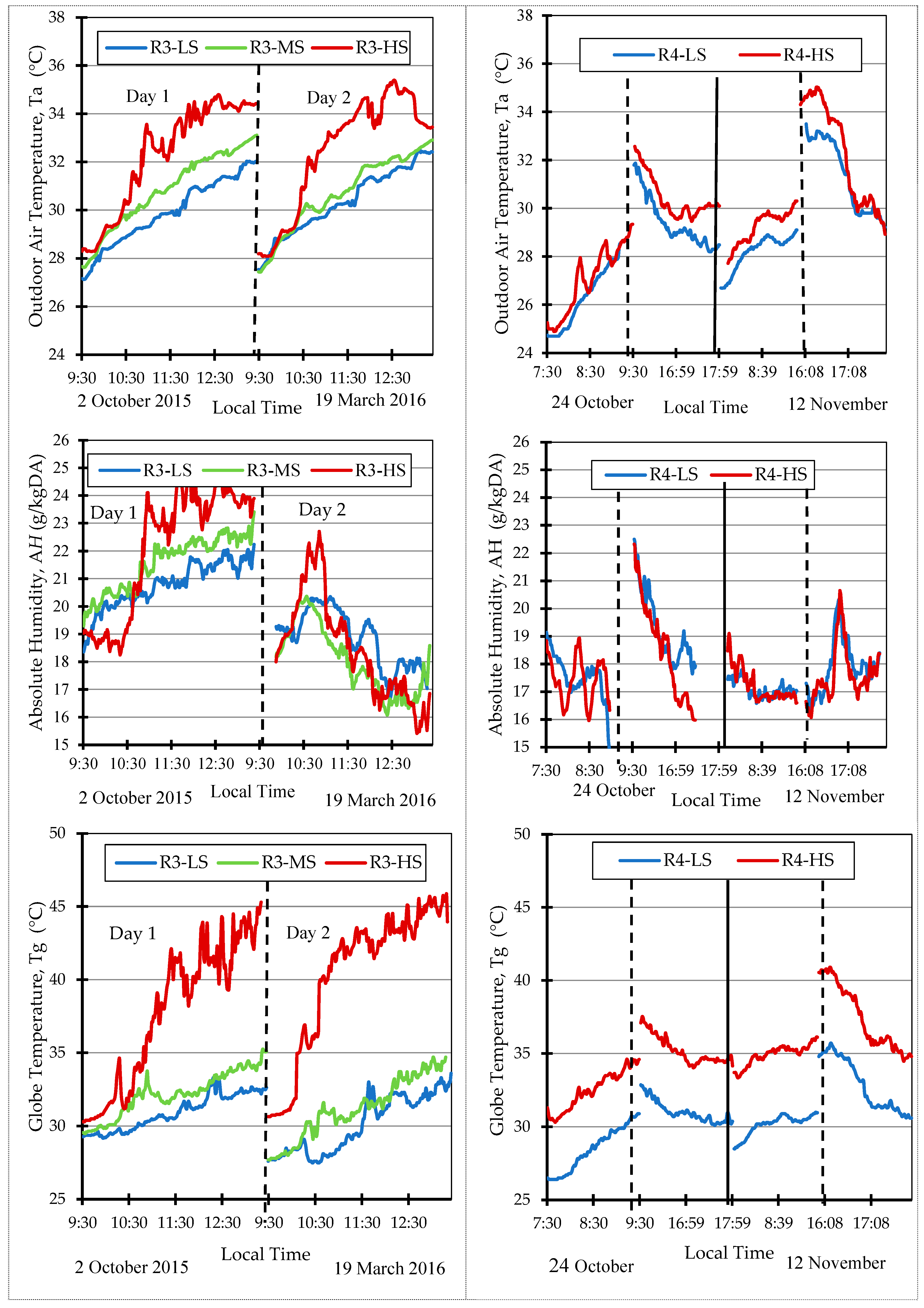
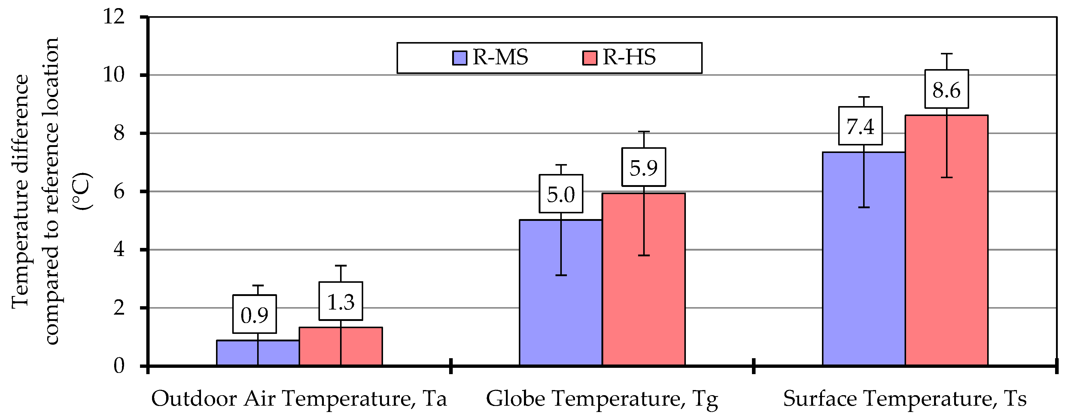
3.2. Relationship between Road Orientation and Outdoor Thermal Environment

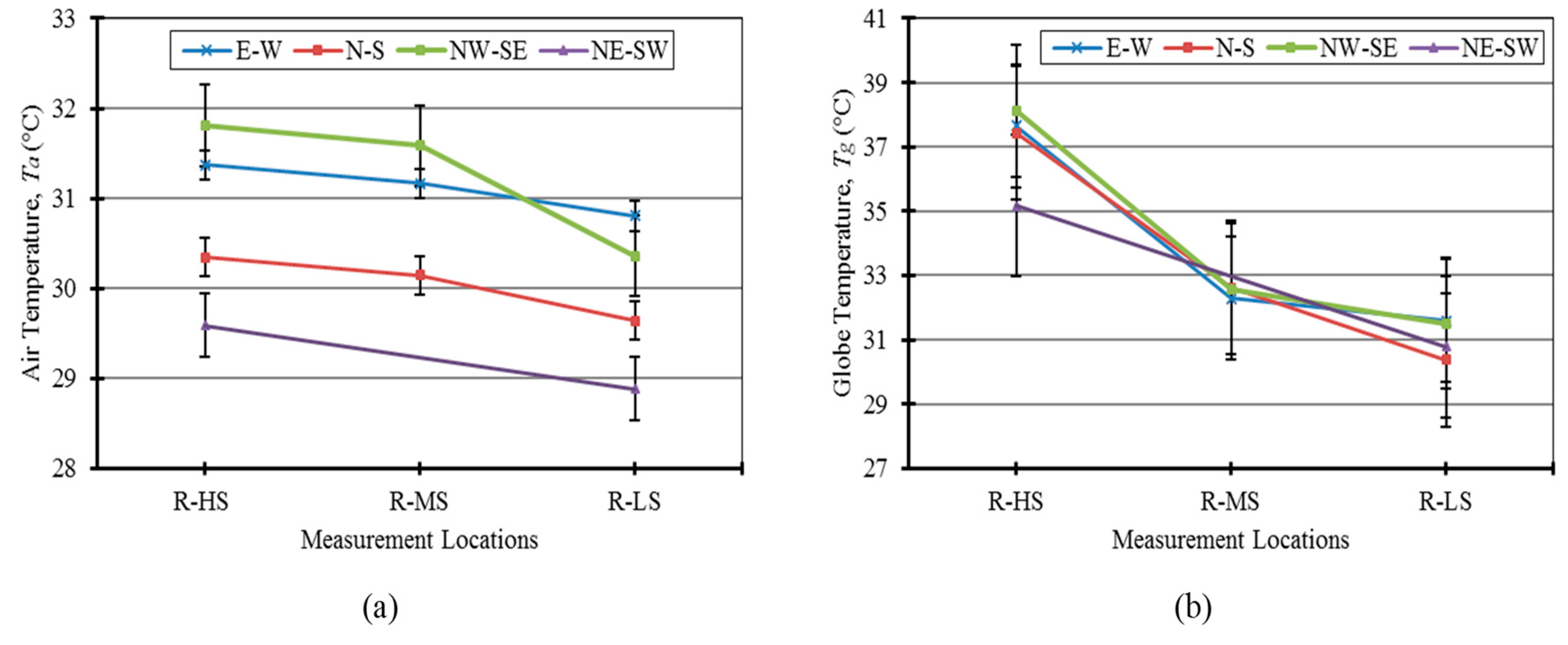
3.2.1. Outdoor air temperature and globe temperature

T_a data was collected over eight sunny days to investigate the effect of road orientation and roadside trees on the outdoor thermal environment. The values are displayed as the overall average of T_a for different roadside tree canopy densities (Figure 11a). The measurement results showed that road orientation affected T_a. At R3-HS, R3 (NW–SE) had the highest average T_a of 31.8 °C, while R3-LS showed a lower value of 30.4 °C, indicating the effect of roadside trees on lowering air temperature. Roads with E–W orientation showed the second-highest average T_a, followed by roads with N–S orientation, while the lowest T_a was measured for roads with NE–SW orientation. These results are consistent with previous simulation results [50], where the average temperature was lowest for 45°-oriented (NE–SW) streets, and highest for 90°-oriented (E–W) streets. According to Ali-Toudert and Mayer [51], E–W streets are slightly warmer than N–S streets due to longer exposure to solar radiation, leading to higher T_a. Overall, the results of this study showed that NW–SE and E–W oriented roads have higher T_a, while N–S and NE–SW roads have lower T_a.

Figure 11b shows the average T_g for various tree canopy conditions. Road orientation affected T_g. At the reference location, T_g exhibited a similar trend to that of T_a, with the highest T_g measured for the NW–SE oriented road (38.1 °C) and the lowest value measured on the NE–SW oriented road (35.2 °C). However, a steep decrease in T_g was observed with increasing canopy cover (R-HS to R-MS to R-LS). At the sites with R-LS, a similar trend was observed for both the E–W and NW–SE oriented roads, where the highest T_g values were 31.6 °C and 31.5 °C, respectively, while the N–S and NE–SW roads showed lower T_g values of 30.4 °C and 30.8 °C, respectively. The higher T_g at E–W and NW–SE oriented roads could be correlated with the higher exposure to solar radiation. Shishegar [52] indicated that NW–SE oriented roads are exposed to direct solar radiation for a longer period of time, especially in the afternoon hours during intense sunlight. In summary, the N–S and NE–SW oriented roads displayed better thermal performance, while E–W and NW–SE oriented roads had higher outdoor air and globe temperatures.

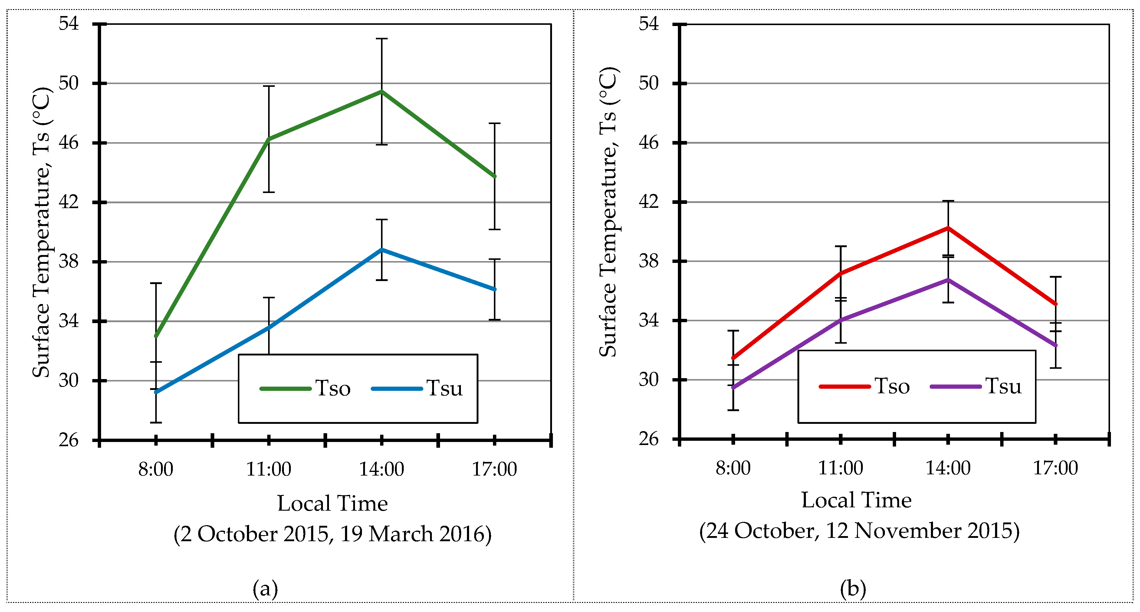
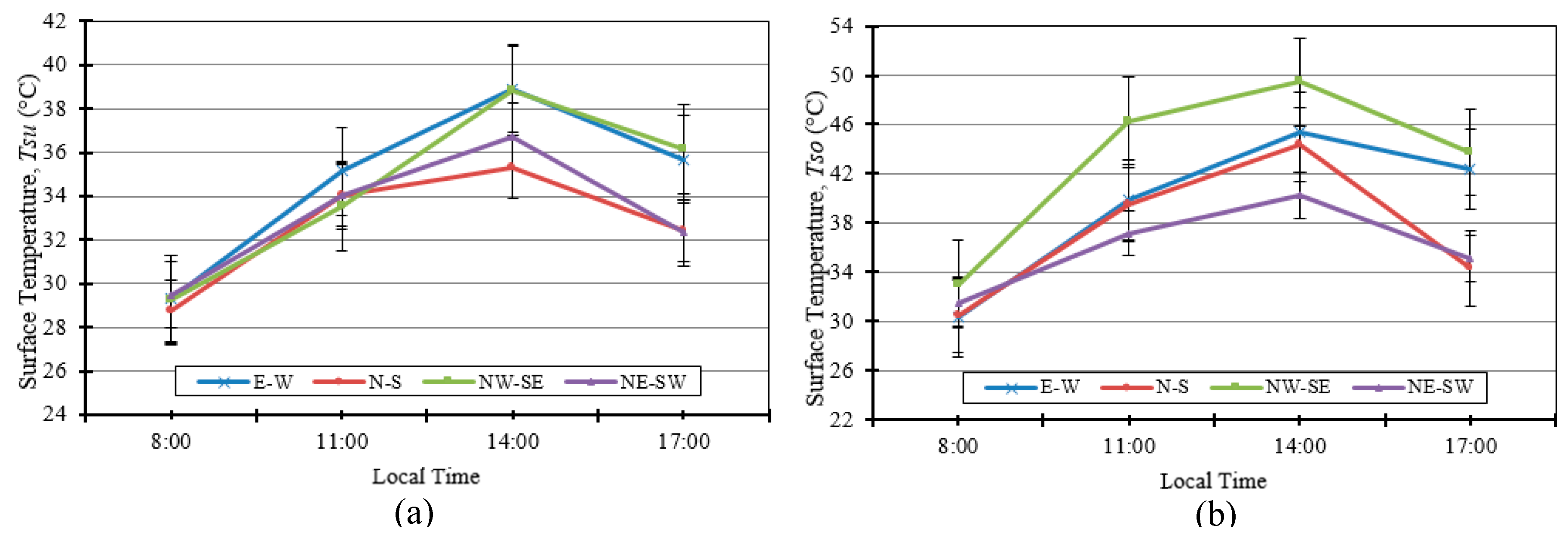
3.2.2. Road Surface Temperature

The average road surface temperature values under tree shade, T_su, and their standard deviations from five points measured for each location are shown in Figure 12a. The measurement results showed that road orientation affected T_su. In the morning, minimal differences were observed between the T_su values measured at different road orientations, while the differences were significant during peak hours in the afternoon. At 14:00, the maximum T_su values were 38.9 °C and 38.8 °C for E–W and NW–SE oriented roads, respectively, while the T_su for a N–S oriented road was only 35.3 °C. The N–S oriented road had the lowest average T_su, while the E–W oriented road had the highest average T_su. Considering the surface temperature under tree shade, the results showed that N–S and NE–SW oriented roads provide a more optimal thermal environment compared to other road orientations.

Figure 12b shows the average road surface temperatures outside of tree shade, T_so, and their standard deviations from five points measured at each location. Similar to the trend of T_su, the difference in T_so for the various road orientations was negligible in the morning and significant during peak hours in the afternoon. The average T_so for the NW–SE oriented road was noticeably higher than the values for the other orientations when the measurement was made outside the tree shade. The maximum and minimum T_so values occurred at 14:00 and 08:00, respectively. We observed that the NW–SE oriented road was the warmest and the NE–SW oriented road was the coolest.

4. Discussion

4.1. Effect of Roadside Tree Configuration

The average T_mrt and PET values at R-LS, R-MS and R-HS areas were calculated from microclimatic measurement data (Figure 13). The data show that T_mrt calculated with the actual wind speed had a significantly greater range (29.3–67.0 °C) than those calculated with the average wind speed (31.2–61.1 °C), although both showed similar average values (Figure 13a,b). This implies that the wind speed influenced the T_mrt value and, consequently, the thermal comfort of pedestrians. The trends in the T_mrt curve were notably similar to those for T_g. Theoretically, faster wind speeds over the globe thermometer result in T_g approaching T_a. In addition, we confirmed that roadside trees provide significant microclimate benefits (by reducing T_mrt), as reported in other similar studies [19,53,54].

During the daytime, PET values at the reference location with R-HS conditions exceeded the upper thermal comfort range limit of 30 °C, and hence, exhibited poor thermal comfort (Figure 13c,d). The PET values were rarely classified as moderate heat stress, except for a short period around 09:50. For the remainder of the measurement period, they fluctuated between strong and extremely strong heat stress. In contrast, PET values under sparse and dense tree canopy with R-MS and R-LS conditions, respectively, provided much better thermal comfort as the heat stress was reduced to a moderate level. The R-LS location showed the lowest PET values, which corresponded to slight heat stress throughout the warmest period of the day. These findings indicate that the presence of roadside trees was able to improve the outdoor thermal comfort tremendously by effectively shielding the incoming solar radiation.

4.2. Effect of Road Orientation

The estimated T_mrt and PET values for the four different road orientations are shown in Figure 14. T_mrt showed similar trends to T_g, with the highest T_mrt at the reference location (R-HS) occurring for the NW–SE oriented road (51.8 °C), while the lowest value was found for the NE–SW oriented road (46.6 °C), as shown in Figure 14a. Roadside trees showed a remarkable cooling effect, indicated by a greatly reduced T_mrt, is when moving from the reference location to sparse (R-MS) and dense (R-LS) tree canopy locations. Hence, T_mrt is dependent on road orientation, and roadside trees greatly improve the thermal environment by reducing T_mrt.

The road orientation also affects the thermal comfort (Figure 14b) when referring to thermal comfort and heat stress categories given by Matzarakis and Mayer [55,56]. At the reference location, PET values were significantly greater for NW–SE and E–W oriented roads. For example, PET values reached extreme heat stress levels in the NW–SE oriented road and strong heat stress in the E–W oriented road. However, for R-MS conditions, the PET values dropped to moderate heat stress levels for the NW–SE oriented road and slight heat stress levels for the other roads. Under R-LS conditions, the N–S oriented road provided the best thermal comfort with PET values corresponding to comfortable or no heat stress levels, while the other roads maintained a slight heat stress level. In addition, roadside trees had a greater cooling potential in NW–SE and E–W oriented roads. By comparing PET at R-LS and R-HS, average PET reductions of 9.7 °C and 9.2 °C were observed for NW–SE and E–W oriented roads, respectively, while the lowest PET reductions of 8.1 °C and 6.2 °C were for the N–S and NE–SW oriented roads, respectively. This demonstrates the dominant effect of the sun’s zenith, which has the same orientation as E–W roads, allowing dense tree canopy to reduce solar radiation exposure during the daytime. Roads with E–W and NW–SE orientation have greater potential for high human heat stress, while the cooling potential and microclimate benefits provides by trees are greater. Therefore, it is important to prioritize roadside tree planting for such roads as the PET can be greatly reduced.

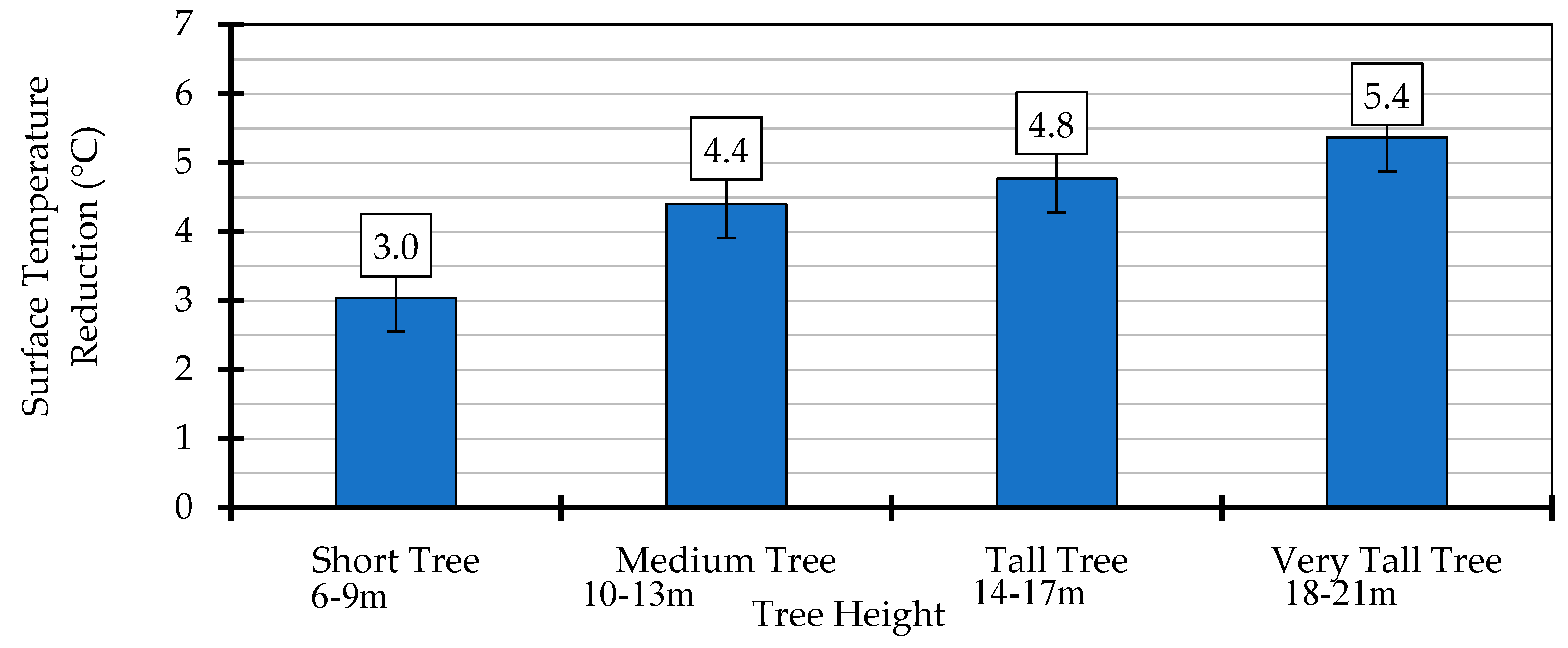
4.3. Effect of Tree Canopy Coverage

Roadside trees provided microclimate and outdoor thermal comfort benefits. On average, planting trees with a dense tree canopy (average SVF of 0.07) can reduce T_mrt significantly by 18.7 °C (35%) and PET by 10.6 °C (25%) compared to the reference location (average SVF of 0.86). Although not as effective as a dense tree canopy, the sparse tree canopy (average SVF of 0.31) also reduced T_mrt and PET considerably, by 15.7 °C and 8.5 °C, respectively, compared to the reference condition. Thermal benefits of roadside trees were revealed in this study, particularly for the hot and humid tropical climate of Kuala Lumpur. Our results are consistent with those of several similar studies that investigated the influences of urban vegetation and roadside trees on microclimates [37,54,57]. Other studies also reported the reduction of PET by trees. For example, in Freiburg, Germany, PET was reduced by 4.6 °C [56] whereas in Campinas, Brazil, tree canopies reduced midday summer PET by 16 °C [47].

4.4. Effect of Tree Canopy Densities on Average Temperature Reduction

On average, the reductions in T_a and T_g under dense tree canopies compared to the reference location with high SVF were 1.3 °C and 5.9 °C, respectively (Figure 15). According to Bowler et al. [58], on average, the air temperature at green sites under canopy is approximately 1 °C cooler than sites without greenery, which confirms the findings of this study. This further affirms the fact that the cooling effect provided by roadside trees improves the outdoor thermal environment by reducing the air and globe temperatures. The density of tree canopy was found to affect T_s. On average, when compared to R-HS, T_s decreased by 7.4 °C and 8.6 °C under R-MS and R-LS conditions, respectively. Nasibeh [23] determined an average reduction of road surface temperature of 7.3 °C under tree shade. Previous studies investigated how canopy density can modify the microclimate environment [17,22,37,59] and showed that dense canopies provide high-quality shade, which effectively reduces the incoming solar radiation during daytime hours. These studies validate the findings of this work, which showed constant reduction in temperatures under dense and sparse canopies compared to the reference location.

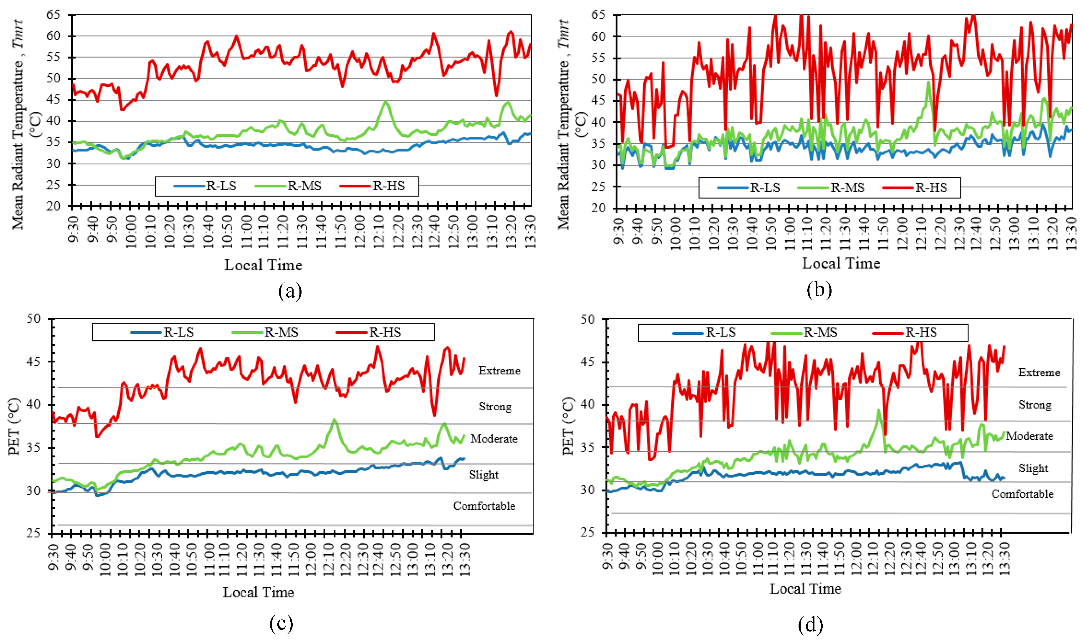
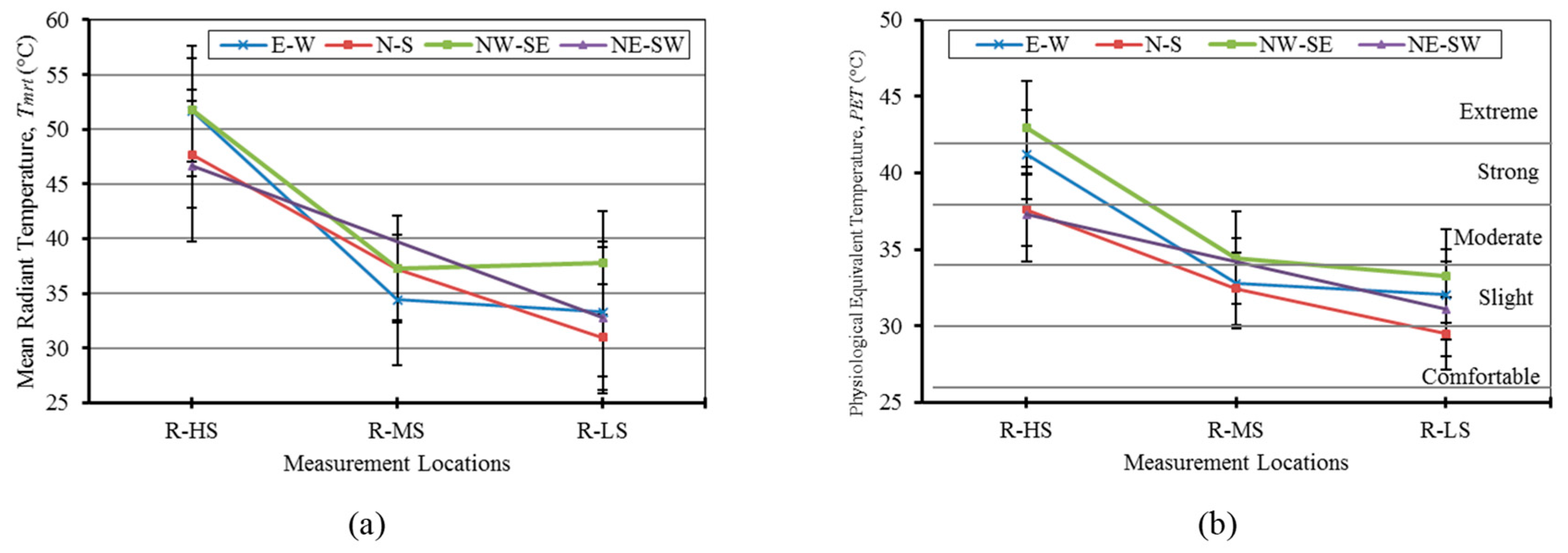
4.5. Microclimate and Outdoor Thermal Comfort

The microclimate benefits from denser tree canopies were predominantly due to the lower SVF and reduction in solar radiation exposure, ground surface heat accumulation, air temperature, and globe temperature. The reduction in solar radiation transmittance decreases the radiant heat incident on a pedestrian [45]. This was indicated by the reduced T_mrt and PET calculated in this study. T_mrt represents the most significant meteorological parameter, which directly affects outdoor thermal comfort [40] and had a stronger correlation than the outdoor air temperature with PET. Therefore, roadside trees are important for both reducing the surrounding air temperature, and greatly reducing T_mrt. Overall, this results in a reduction in outdoor thermal stress.

In addition to tree canopy shade, the tree transpiration process also benefits the microclimate, which has been determined via sap flow measurements [38]. Although sap flow was not investigated in this study, higher AH values in areas of dense and sparse tree canopy compared to the reference location were measured. This data suggested that the release of water vapor into the atmosphere from the transpiration process increased the air humidity. Therefore, it could also be assumed that the lower air temperature measured under the tree canopies was partly due to the transpiration of the trees [60]. However, McNall et al. [61] indicated that higher air humidity is not considered a benefit for pedestrians at high levels of physical activity, as it reduces the efficiency of sweat evaporation from the human body.

Chen et al. [62] proposed that the effect of urban trees on outdoor thermal comfort and daytime microclimate (e.g., air temperature, surface temperature, and mean radiant temperature) is the combined result of two counteracting mechanisms: (i) the reduction in road surface temperature due to tree shade; and (ii) the reduced wind speed due to the tree canopy (which results in less ventilation and an increase in T_a). However, this study demonstrated that the first effect was dominant, as nearly all of the temperatures measured under the tree canopy were significantly lower than the reference values. Similarly, a study by Cohen et al. [57] showed that wind speed did not contribute significantly to the outdoor PET as wind speeds were small and could not outweigh the thermal benefit of trees on other parameters, such as globe temperature and solar radiation.

Previous studies have shown that the road orientation affects the road thermal environment [39,51]. The results of this study confirmed that the road orientation significantly affects the thermal environment and road microclimate. In our case, E–W and NW–SE oriented roads had a greater potential for high human thermal stress, whereas the opposite was shown for N–S and NE–SW roads. The findings of this study align with those reported by Ali-Toudert and Mayer [51] for E–W and N–S oriented roads, but not for NW–SW oriented roads. Their simulation results showed that intermediate road orientations (NW–SE and NE–SW) offered thermal conditions similar to N–S oriented roads. In this study, however, NW–SE oriented road showed the highest temperature due to the exposure to intense sunlight during afternoon hours [51]. This could be because the study by Ali-Toudert and Mayer [51] was conducted in a temperate climate versus the tropical climate this study was performed in. This would suggest that results from different climate regions are not interchangeable, as we originally hypothesized. Depending on the level and duration of solar radiation exposure, road orientation affects the microclimate and outdoor thermal comfort. E–W oriented roads allow longer duration of solar exposure compared to N–S oriented roads [39,63]. In the case of intermediate orientations, NW–SE oriented roads are exposed to high-intensity solar radiation in the afternoon, resulting in the high temperatures measured here. Norton et al. [64] suggested that it should be a priority to plant roadside trees along E–W oriented roads; however, roadside trees provide benefits for the microclimate and outdoor thermal comfort, regardless of the orientation of the road.

5. Conclusions

There are three main conclusions based on the research objectives and findings of this study. First, mitigation effects of roadside trees on outdoor meteorological parameters were shown, with T_a, T_g, and T_s values decreasing on average by 4%, 16%, and 21%, respectively, for dense roadside tree canopies comparing to the reference location. Under sparse tree canopy, the reduction in T_a, T_g, and T_s values was slightly lower, with values of 3%, 14%, and 18%, respectively. In contrast, higher AH values were observed for areas of higher tree density. Despite the tendency of previous similar studies to focus on the reduction of T_a, the reduction of T_g and T_s were observed, suggesting that radiation was the dominant factor affecting the thermal environment, where the tree canopy effectively blocks the incoming direct solar radiation and cools the environment. In addition, taller and more mature trees provided a larger shade area than smaller trees, resulting in a larger cooling effect. In this study, tall trees (18–21 m) reduced T_s by 14%, compared with a reduction of 8% under short trees (6–9 m). Therefore, we recommend the use of mature tall trees with a dense canopy for future urban road planning to ensure the maximum benefits.

Second, different road orientations were found to influence the road thermal environment. T_a, T_g, T_s, and T_mrt were all lower for N–S and NE–SW oriented roads, whereas E–W and NW–SE oriented roads had the highest temperatures at the studied latitude and solar path. Therefore, urban planners could consider building fewer E–W and NW–SE oriented roads in new urban development areas. However, the microclimate benefits of roadside trees were still significant, irrespective of the road orientation. For example, the presence of trees with high canopy density along N–S roads reduced midday T_g and T_s by a considerable 7.0 °C and 3.8 °C, respectively, compared to the reference location. Notably, T_s was 7.1 °C lower on average for the NW–SE orientated road under tree shade compared to the uncovered road. T_mrt showed similar trends to other parameters (i.e., lower values for N–S and NE–SW roads).

Finally, we confirmed that roadside trees contributed to lower temperatures and better thermal environments by investigating the thermal comfort level expressed by the PET, which showed a decrease from strong heat stress to slight heat stress with the presence of roadside trees. Specifically, PET decreased by 25% and 20% under dense and sparse canopies, respectively, compared to the reference location. Although N–S and NE–SW roads had lower PET values, the cooling effects of roadside trees were observed for NW–SE and E–W roads, with an average PET reduction of 23%, compared to 18% and 17% for N–S and NE–SW oriented roads, respectively.

The findings of this study are expected to be beneficial and applicable for planning similar future studies, as they provide evidence for urban planners and policy makers on the extent and magnitude of the cooling effects of roadside trees. The proposed measure of planting roadside trees is useful for both new urban developments and existing urban areas in Malaysia. However, this study has limitations in terms of daily measurement periods and could be expanded and improved to incorporate more elements. This could include incorporating and comparing different tree species with distinct features, such as leaf size, branching arrangement, and canopy shape. In addition, various road widths and road pavement surface materials could be considered to investigate their effects on the road thermal environment. Furthermore, future studies could incorporate additional data collection techniques, such as daily continuous measurement and mobile measurements, in order to visualize the diurnal and nocturnal effects of roadside trees and to cover a larger area.

References

1. McMichael, A.J.; Woodruff, R.E.; Hales, S. Climate change and human health: Present and future risks. Lancet 2006, 367, 859–869. [Google Scholar] [CrossRef]
2. Semenza, C.J. Climate change and human health. Int. J. Environ. Res. Pub. Health. 2014, 11, 7347–7353. [Google Scholar] [CrossRef] [PubMed] [Green Version]
3. Dhainaut, J.F.; Claessens, Y.E.; Ginsburg, C.; Riou, B. Unprecedented heat-related deaths during the 2003 heat wave in Paris: Consequences on emergency departments. Crit. Care. 2004, 8, 1–2. [Google Scholar] [CrossRef] [PubMed] [Green Version]
4. Smoyer, K.E.; Rainham, D.G.C.; Hewko, J.N. Heat-stress-related mortality in five cities in Southern Ontario: 1980–1996. Int. J. Biometeorol. 2000, 44, 190–197. [Google Scholar] [CrossRef]
5. Oke, T.R. Chandler, TJ 1965: The climate of London. London: Hutchinson. Prog. Phys. Geogr. 2009, 33, 437–442. [Google Scholar] [CrossRef]
6. Mills, G. Luke Howard and the Climate of London. Weather 2003, 63, 153–157. [Google Scholar] [CrossRef]
7. Roth, M. Urban Heat Islands. In Handbook of Environmental Fluid Dynamics; Fernando, H.J.S., Ed.; CRC Press/Taylor & Francis Group, LLC.: Boca Raton, FL, USA, 2013. [Google Scholar]
8. Luber, G.; McGeehin, M. Climate change and extreme heat events. Am. J. Prev. Med. 2008, 35, 429–435. [Google Scholar] [CrossRef]
9. Oke, T.R. City size and the urban heat island. Atmos. Environ. 1973, 7, 769–779. [Google Scholar] [CrossRef]
10. Oke, T.R. Street design and urban canopy layer climate. Energy Build. 1988, 11, 103–113. [Google Scholar] [CrossRef]
11. Tran, H.; Uchihama, D.; Ochi, S.; Yasuoka, Y. Assessment with satellite data of the urban heat island effects in Asian mega cities. Int. J. Appl. Earth Obs. Geoinf. 2006, 8, 34–48. [Google Scholar] [CrossRef]
12. Gartland, L. Heat Islands: Understanding and Mitigating Heat in Urban Areas; Routledge: London, UK, 2012. [Google Scholar]
13. Honjo, T. Thermal comfort in outdoor environment. Glob. Environ. Res. AIRIES. 2009, 13, 43–47. [Google Scholar]
14. Hass-Klau, C. Impact of pedestrianization and traffic calming on retailing: A review of the evidence from Germany and the UK. Transp. Policy. 1993, 1, 21–31. [Google Scholar] [CrossRef]
15. Hakim, A.A.; Petrovitch, H.; Burchfiel, C.M.; Ross, G.W.; Rodriguez, B.L.; White, L.R.; Yano, K.; Curb, J.D.; Abbott, R.D. Effects of Walking on Mortality among Nonsmoking Retired Men. N. Engl. J. Med. 1998, 100, 9–13. [Google Scholar] [CrossRef] [PubMed]
16. Kikuchi, A.; Hataya, N.; Mochida, A.; Yoshino, H.; Tabata, Y.; Watanabe, H.; Jyunimura, Y. Field study of the influences of roadside trees and moving automobiles on turbulent diffusion of air pollutants and thermal environment in urban street canyons. In Proceedings of the 6th International Conference on Indoor Air Quality, Ventilation & Energy Conservation in Buildings (IAQVEC ′07), Sendai, Japan, 28–31 October 2007. [Google Scholar]
17. Narita, K.; Sugawara, H.; Honjo, T. effects of roadside trees on the thermal environment within a street canyon. Geogr. Rep. Tokyo Metrop. Univ. 2008, 43, 41–48. [Google Scholar]
18. Tsiros, I.X. Assessment and energy implications of street air temperature cooling by shade tress in Athens (Greece) under extremely hot weather conditions. Renew. Energy. 2010, 35, 1866–1869. [Google Scholar] [CrossRef]
19. Park, M.; Hagishima, A.; Tanimoto, J.; Narita, K.-I. Effect of urban vegetation on outdoor thermal environment: Field measurement at a scale model site. Build. Environ. 2012, 56, 38–46. [Google Scholar] [CrossRef]
20. Wong, P.P.Y.; Lai, P.C.; Low, C.T.; Chen, S.; Hart, M. The impact of environmental and human factors on urban heat and microclimate variability. Build. Environ. 2016, 95, 199–208. [Google Scholar] [CrossRef] [Green Version]
21. Wong, N.H.; Jusuf, S.K. Study on the microclimate condition along a green pedestrian canyon in Singapore. Archit. Sci. Rev. 2010, 53, 196–212. [Google Scholar] [CrossRef]
22. Shahidan, M.F.; Jones, P.J.; Gwilliam, J.; Salleh, E. An evaluation of outdoor and building environment cooling achieved through combination modification of trees with ground materials. Build. Environ. 2012, 58, 245–257. [Google Scholar] [CrossRef]
23. Nasibeh, F.M. Effects of road geometry and roadside trees on urban road thermal performance in Penang. Doctor Philosophy, Universiti Sains Malaysia, Penang, Malaysia, 2016. [Google Scholar]
24. Yang, G.; Yu, Z.; Jørgensen, G.; Vejre, H. How can urban blue-green space be planned for climate adaption in high-latitude cities? A seasonal perspective. Sustain. Cities Soc. 2020, 53, 152–162. [Google Scholar] [CrossRef]
25. Fan, H.Y.; Yu, Z.W.; Yang, G.Y.; Liu, T.Y. How to cool hot-humid (Asian) cities with urban trees? An optimal landscape size perspective. Agric. For. Meteorol. 2019, 265, 338–348. [Google Scholar] [CrossRef]
26. Yu, Z.; Xu, S.; Zhang, Y.; Jørgensen, G.; Vejre, H. Strong contributions of local background climate to the cooling effect of urban green vegetation. Sci. Rep. 2018, 8, 6798. [Google Scholar] [CrossRef] [PubMed]
27. Givoni, B. Impact of planted areas on urban environmental quality: A review. Atmos. Environ. Part B Urban Atmos. 1991, 25, 289–299. [Google Scholar] [CrossRef]
28. Gonçalves, A.; Castro Ribeiro, A.; Maia, F.; Nunes, L.; Feliciano, M. Influence of Green Spaces on Outdoors Thermal Comfort—Structured Experiment in a Mediterranean Climate. Climate 2019, 7, 20. [Google Scholar] [CrossRef] [Green Version]
29. Takács, Á.; Kiss, M.; Hof, A.; Tanács, E.; Gulyás, Á.; Kántor, N. Microclimate Modification by Urban Shade Trees – An Integrated Approach to Aid Ecosystem Service Based Decision-making. Procedia Environ. Sci. 2016, 32, 97–109. [Google Scholar] [CrossRef] [Green Version]
30. Pauleit, S. Urban street tree plantings: identifying the key requirements. Proc. Inst. Civ. Eng. - Munic. Eng. 2003, 56, 43–50. [Google Scholar] [CrossRef]
31. Dumbaugh, E. Safe streets, livable streets. J. Am. Plan. Assoc. 2005, 71, 283–300. [Google Scholar] [CrossRef]
32. Ware, G.H. Ecological bases for selecting urban trees. J. Arboric. 1994, 20, 98–103. [Google Scholar]
33. Thaiutsa, B.; Puangchit, L.; Kjelgren, R.; Arunpraparut, W. Urban green space, street tree and heritage large tree assessment in Bangkok, Thailand. Urban For. Urban Green. 2008, 7, 219–229. [Google Scholar] [CrossRef]
34. Jim, C.Y. A planning strategy to augment the diversity and biomass of roadside trees in urban Hong Kong. Landsc. Urban Plan. 1999, 44, 13–32. [Google Scholar] [CrossRef]
35. Köppen, W.; Volken, E.; Brönnimann, S. The thermal zones of the Earth according to the duration of hot, moderate and cold periods and to the impact of heat on the organic world. Meteorol. Z. 2011, 20, 351–360. [Google Scholar] [CrossRef] [PubMed]
36. Khalid, W.; Zaki, S.A.; Rijal, H.B.; Yakub, F. Investigation of comfort temperature and thermal adaptation for patients and visitors in Malaysian hospitals. Energy Build. 2019, 183, 484–499. [Google Scholar] [CrossRef]
37. Costa, A.; Labaki, L.; Araújo, V. A methodology to study the urban distribution of air temperature in fixed points. Proceeding of 2nd PALENC Conference and 28th AIVC Conference on Building Low Energy Cooling and Advanced Ventilation Technologies in the 21st Century, Crete island, Greece, 27–29 September 2007; pp. 227–230. [Google Scholar]
38. Jan, F.-C.; Hsieh, C.-M.; Ishikawa, M. Influence of street tree density on transpiration in a subtropical climate. Environ. Nat. Resour. Res. 2012, 2, 84–95. [Google Scholar] [CrossRef]
39. Sanusi, R.; Johnstone, D.; May, P.; Livesley, S.J. Street Orientation and Side of the Street Greatly Influence the Microclimatic Benefits Street Trees Can Provide in Summer. J. Environ. Qual. 2016, 45, 167–174. [Google Scholar] [CrossRef] [Green Version]
40. Makaremi, N.; Salleh, E.; Jaafar, M.Z.; GhaffarianHoseini, A. Thermal comfort conditions of shaded outdoor spaces in hot and humid climate of Malaysia. Build. Environ. 2012, 48, 7–14. [Google Scholar] [CrossRef]
41. Matzarakis, A.; Rutz, F.; Mayer, H. Modelling radiation fluxes in simple and complex environments: Basics of the RayMan model. Int. J. Biometeorol. 2010, 54, 131–139. [Google Scholar] [CrossRef] [Green Version]
42. British Standards Institution. ISO 7726:2001; British Standards Institution: London, UK, 2001. [Google Scholar]
43. Lin, T.P.; Matzarakis, A. Tourism climate and thermal comfort in Sun Moon Lake, Taiwan. Int. J. Biometeorol. 2008, 52, 281–290. [Google Scholar] [CrossRef]
44. Matzarakis, A.; Mayer, H. Another kind of environmental stress: thermal stress. WHO Collaborating Centre for Air Quality Management and Air Pollution Control. NEWSLETTERS 1996, 18, 7–10. [Google Scholar] [CrossRef]
45. Ahmed, K.S. Comfort in urban spaces: Defining the boundaries of outdoor thermal comfort for the tropical urban environments. Energy Build. 2003, 35, 103–110. [Google Scholar] [CrossRef]
46. Shashua-Bar, L.; Pearlmutter, D.; Erell, E. The influence of trees and grass on outdoor thermal comfort in a hot-arid environment. Int. J. Climatol. 2011, 31, 1498–1506. [Google Scholar] [CrossRef]
47. Loyde, V.A.; Labaki, L.C.; Matzarakis, A. Effect of tree planting design and tree species on human thermal comfort in the tropics. Lands. Urban Plan. 2015, 138, 99–109. [Google Scholar]
48. Morakinyo, T.E.; Kong, L.; Lau, K.K.L.; Yuan, C.; Ng, E. A study on the impact of shadow-cast and tree species on in-canyon and neighborhood’s thermal comfort. Build. Environ. 2017, 115, 1–17. [Google Scholar] [CrossRef]
49. Rantzoudi, E.C.; Georgi, J.N. Correlation between the geometrical characteristics of streets and morphological features of trees for the formation of tree lines in the urban design of the city of Orestiada, Greece. Urban Ecosyst. 2017, 20, 1081–1093. [Google Scholar] [CrossRef]
50. Cao, A.; Li, Q.; Meng, Q. Effects of orientation of urban roads on the local thermal environment in Guangzhou city. Procedia Eng. 2015, 121, 2075–2082. [Google Scholar] [CrossRef] [Green Version]
51. Ali-Toudert, F.; Mayer, H. Numerical study on the effects of aspect ratio and orientation of an urban street canyon on outdoor thermal comfort in hot and dry climate. Build. Environ. 2006, 41, 94–108. [Google Scholar] [CrossRef]
52. Shishegar, N. Street Design and Urban Microclimate: Analyzing the effects of street geometry and orientation on airflow and solar access in urban canyons. J. Clean Energy Technol. 2013, 1, 52–56. [Google Scholar] [CrossRef]
53. Johansson, E.; Emmanuel, R. The influence of urban design on outdoor thermal comfort in the hot, humid city of Colombo, Sri Lanka. Int. J. Biometeorol. 2006, 51, 119–133. [Google Scholar] [CrossRef]
54. Sanusi, R.; Johnstone, D.; May, P.; Livesley, S.J. Microclimate benefits that different street tree species provide to sidewalk pedestrians relate to differences in Plant Area Index. Landsc. Urban Plan. 2017, 157, 502–511. [Google Scholar] [CrossRef]
55. Krüger, E.; Rossi, F.; Drach, P. Calibration of the physiological equivalent temperature index for three different climatic regions. Int. J. Biometeorol. 2017, 61, 1323–1336. [Google Scholar] [CrossRef]
56. Mayer, H.; Kuppe, S.; Holst, J.; Imbery, F.; Matzarakis, A. Human thermal comfort below the canopy of street trees on a typical Central European summer day. Meteorol. Inst. 2009, 18, 211–219. [Google Scholar]
57. Cohen, P.; Potchter, O.; Matzarakis, A. Daily and seasonal climatic conditions of green urban open spaces in the Mediterranean climate and their impact on human comfort. Build. Environ. 2012, 51, 285–296. [Google Scholar] [CrossRef]
58. Bowler, D.E.; Buyung-Ali, L.; Knight, T.M.; Pullin, A.S. Urban greening to cool towns and cities: A systematic review of the empirical evidence. Landsc. Urban Plan. 2010, 97, 147–155. [Google Scholar] [CrossRef]
59. Faghih Mirzaei, N.; Fairuz Syed Fadzil, S.; Binti Taib, N.; Abdullah, A. Micro-scale evaluation of the relationship between road surface and air temperature with respect to various surrounding greenery covers. Res. J. Appl. Sci. Eng. Technol. 2015, 11, 454–459. [Google Scholar] [CrossRef]
60. Shashua-Bar, L.; Hoffman, M.E. Vegetation as a climatic component in the design of an urban street. An empirical model for predicting the cooling effect of urban green areas with trees. Energy Build. 2000, 31, 221–225. [Google Scholar] [CrossRef]
61. McNall, P., Jr.; Jaax, J.; Rohles, F.; Nevins, R.; Springer, W. Thermal comfort (thermally neutral) conditions for three levels of activity. ASHRAE Trans. 1967, 73, 6–10. [Google Scholar]
62. Chen, H.; Ooka, R.; Kato, S. Study on optimum design method for pleasant outdoor thermal environment using genetic algorithms (GA) and coupled simulation of convection, radiation and conduction. Build. Environ. 2008, 43, 18–30. [Google Scholar] [CrossRef]
63. Oliveira, S.; Andrade, H.; Vaz, T. The cooling effect of green spaces as a contribution to the mitigation of urban heat: A case study in Lisbon. Build. Environ. 2011, 46, 2186–2194. [Google Scholar] [CrossRef]
64. Norton, B.A.; Coutts, A.M.; Livesley, S.J.; Harris, R.J.; Hunter, A.M.; Williams, N.S.G. Planning for cooler cities: A framework to prioritise green infrastructure to mitigate high temperatures in urban landscapes. Landsc. Urban Plan. 2015, 134, 127–138. [Google Scholar] [CrossRef]
Figure 1. Variation in monthly average outdoor climate conditions: (a) outdoor air temperature (°C) and relative humidity (%); (b) solar radiation (W/m²); and (c) total precipitation (mm), measured at the MJIIT building in Kuala Lumpur from April 2015 to March 2016, with standard deviations represented by error bars. The measurement periods are shaded in light green.
Sustainability 12 01053 g001
Figure 2. Variation in diurnal air temperature (°C) and solar radiation (W/m2) on field-measurement days: (a) 8 April 2015 and 18 May 2015; (b) 28 May 2015 and 3 June 2015; (c) 2 October 2015 and 19 March 2016; and (d) 24 October 2015 and 12 November 2015.
Sustainability 12 01053 g002
Figure 3. Photographs of survey locations (a) R1, (b) R2, (c) R3, and (d) R4. The top row (a1, b1, c1, d1) shows plan views (Google Earth screenshot taken 19 December 2017), and the bottom row (a2, b2, c2, d2) shows the corresponding Google street view images. (e) Satellite map showing the four survey locations.
Sustainability 12 01053 g003
Figure 4. Photographs of the (a) Pterocarpus indicus and (b) Samanea saman trees located at the studied sites. The images were supplied by the Forest Research Institute Malaysia.
Sustainability 12 01053 g004
Figure 5. Photograph indicating representative locations of surface temperature (Ts) measurements under (green circles, Tsu) and outside (red circle, Tso) shade from trees at R2.
Sustainability 12 01053 g005
Figure 6. Schematic plan of the selected locations (a) R1, (b) R2, (c) R3, and (d) R4, with approximate positions of instrument setups. Three measurement stations (ST1, ST2, and ST3) were installed at each location. The periodic measurement for surface temperature under tree shade (Tsu) and outside tree shade (Tso) was also measured at each location.
Sustainability 12 01053 g006
Figure 7. Street view and fisheye photos of measurement locations (a) R1, (b) R2, (c) R3, and (d) R4. At R1, (a1) to (a3) are the street view photos, SVF value for (a4) (R1-LS) is 0.04, (a5) (R1-MS) is 0.28, and (a6) (R1-HS) is 0.08. At R2, (b1) to (b3) are the street view photos, SVF value for (b4) (R2-LS) is 0.08, (b5) (R2-MS) is 0.35, and (b6) (R2-HS) is 0.85. At R3, (c1) to (c3) are the street view photos, SVF value for (c4) (R3-LS) is 0.08, (c5) (R3-MS) is 0.29, and (c6) (R3-HS) is 0.92. At R4, (d1) and (d2) are the street view photos, SVF value for (d3) (R4-LS) is 0.09, and (d4) (R4-HS) is 0.88.
Sustainability 12 01053 g007
Figure 8. Variation of outdoor microclimate parameters for locations (a) R1 and (b) R2, where the error bars represent standard deviation. The vertical dotted lines separate the two measurement days.
Sustainability 12 01053 g008aSustainability 12 01053 g008b
Figure 9. Variation in outdoor microclimate parameters at location (a) R3 and (b) R4, where the error bars represent standard deviation. The vertical dotted lines separate the two measurement days or measurement periods on the same day.
Sustainability 12 01053 g009aSustainability 12 01053 g009b
Figure 10. Average reduction in road surface temperature (°C) as a function of roadside tree height (m) compared to road surface temperatures outside the shaded area. The measurement periods were 8 April, 18 May, 28 May, 2 October, 24 October, 12 November 2015 and 19 March 2016.
Sustainability 12 01053 g010
Figure 11. Overall average (a) outdoor air temperature, and (b) globe temperature for four selected urban roads with different orientations and tree canopy densities. The standard deviations are represented by the error bars. The measurement periods were 8 April, 18 May, 28 May, 2 October, 24 October, 12 November 2015, and 19 March 2016.
Sustainability 12 01053 g011
Figure 12. Comparison of average road surface temperatures for four different road orientations measured (a) under tree shade, and (b) outside of tree shade. The standard deviations are represented by the error bars. The measurement periods were 8 April, 18 May, 28 May, 2 October, 24 October, 12 November 2015, and 19 March 2016.
Sustainability 12 01053 g012
Figure 13. Tmrt calculated using (a) averaged wind speed and (b) actual wind speed. Physiological equivalent temperature (PET) calculated using (c) averaged wind speed and (d) actual wind speed. The level of heat stress is indicated on the right-hand side of the figure, where the horizontal lines indicate the boundaries for each heat stress level.
Sustainability 12 01053 g013
Figure 14. Average (a) Tmrt and (b) PET for the four selected urban roads with different orientations. The standard deviations are represented by the error bars. The level of heat stress is shown on the right-hand side of (b), where the horizontal lines indicate the boundaries for each heat stress level.
Sustainability 12 01053 g014
Figure 15. Average reduction in air temperature, globe temperature, and road surface temperature under sparse (R-MS) and dense (R-LS) tree canopies compared to the reference area (R-HS). The measurement periods were 8 April, 18 May, 28 May, 2 October, 24 October, 12 November 2015, and 19 March 2016.
Sustainability 12 01053 g015