Exploring the Spatial-Temporal Relationship between Rainfall and Traffic Flow: A Case Study of Brisbane, Australia

School of Civil Engineering, The University of Queensland, St. Lucia, Brisbane 4072, Australia
*
Author to whom correspondence should be addressed.
Sustainability 2020, 12(14), 5596; https://0-doi-org.brum.beds.ac.uk/10.3390/su12145596
Submission received: 8 June 2020
/
Revised: 8 July 2020
/
Accepted: 9 July 2020
/
Published: 11 July 2020
(This article belongs to the Section Sustainable Transportation)
Abstract
:The impact of inclement weather on traffic flow has been extensively studied in the literature. However, little research has unveiled how local weather conditions affect real-time traffic flows both spatially and temporally. By analysing the real-time traffic flow data of Traffic Signal Controllers (TSCs) and weather information in Brisbane, Australia, this paper aims to explore weather’s impact on traffic flow, more specifically, rainfall’s impact on traffic flow. A suite of analytic methods has been applied, including the space-time cube, time-series clustering, and regression models at three different levels (i.e., comprehensive, location-specific, and aggregate). Our results reveal that rainfall would induce a change of the traffic flow temporally (on weekdays, Saturday, and Sunday and at various periods on each day) and spatially (in the transportation network). Particularly, our results consistently show that the traffic flow would increase on wet days, especially on weekdays, and that the urban inner space, such as the central business district (CBD), is more likely to be impacted by inclement weather compared with other suburbs. Such results could be used by traffic operators to better manage traffic in response to rainfall. The findings could also help transport planners and policy analysts to identify the key transport corridors that are most susceptible to traffic shifts in different weather conditions and establish more weather-resilient transport infrastructures accordingly.
1. Introduction
The recent expansion of urban areas has brought the diversity of transportation modes in order to meet the increasing traffic demands in daily life, which accordingly leads to a larger amount of traffic flow on roads [1]. To deal with the various transportation modes, a deep understanding of traffic demand and performance is critical [2]. Typically, traffic information contains many attributes such as speed, flow, and density, among which traffic flow is normally considered as the essential element that can illustrate the efficiency of traffic management and control [3].
The negative influence of adverse weather on traffic situation is becoming a major concern to transportation authorities and agencies [4]. First, the external conditions, such as the roughness of the road surface that can affect the skid of vehicles, could be altered, which may influence driving behaviour and road safety accordingly. Meanwhile, the traffic pattern in adverse weather might be different in contrast to the situation in a dry weather condition [5]. Overall, inclement weather affects transportation in three aspects—demand, safety, and capacity (flow of traffic)—which has been extensively investigated in the literature [4,5,6,7,8,9]. However, many of the studies primarily focused on the fluctuation of the quantities of traffic flow that are affected by inclement weather and very few studies explored the impact of wet weather conditions on temporal and spatial patterns of traffic flow. Furthermore, although some efforts have been made to quantify the spatial-temporal patterns of real-time traffic flow [10,11,12,13], few of them associated the spatial-temporal patterns of real-time traffic flow with weather information (especially the inclement weather information).
In this paper, to investigate weather’s impact on the spatial-temporal feature of traffic flow, which describes how the traffic changes in the time-space domain [14], we consider one commonly used weather parameter—precipitation, which implies the amount of rainfall and snowfall [15]. The utility of combining traffic flow with weather information is that the temporal-spatial characteristics of traffic flow under diverse weather conditions can be revealed, highlighted, and converted into distribution patterns at the spatial and temporal dimension. To fully explore these characteristics, we adopt a spatial-temporal analytic approach, which can both qualitatively visualise and quantitatively model the spatial-temporal relationship between weather (rainfall in this study) and traffic flow.
Specifically, we first explore the distribution patterns of traffic flow in different weather conditions using space-time cube and time-series clustering methods to visualise the spatial-temporal patterns of traffic flow under dry/wet weather conditions, and then, detect weather’s impact on traffic flow using statistical models, and identify the time and the location at which traffic flow was impacted by weather; finally, we quantify weather’s impact on traffic flow at three different levels (i.e., comprehensive, location-specific, and aggregate). The findings gained from the research can help transport planners and policy analysts to identify key transport corridors that are most susceptible to traffic flow changes in different weather conditions and establish more weather-resilient transport infrastructures accordingly.
The rest of the paper is organized as follows. Section 2 reviews relevant studies in the literature. Section 3 introduces the study region and data sources used in this study. Section 4 describes the methodologies employed in analysing the data. Section 5 presents the distribution pattern visualisation of traffic flow, the modelling analysis, and its interpretation. Finally, in Section 6 we discuss the findings, limitations, and future work.
2. Literature Review
The impact of inclement weather on traffic flow has been extensively investigated in the literature. In general, previous studies consistently indicated that heavy rain and snow can reduce road capacity and traffic speed, and increase vehicle crash possibility [4,5,6,7,8,9]. Maze et al. [16] found that inclement weather’s impact on traffic depends on the intensity of inclement weather and the type of travelling mode. Prevedouros and Chang [17] observed that the intersection operations can be affected by wet weather conditions in three specific aspects (flow and capacity of the roads, the effective time of green light, and the progression), which may deteriorate the level of service. Agbolosu-Amison et al. [18] studied the influence of inclement weather on saturation flow, and the results show that the saturation flow has a significant correlation with inclement weather.
Due to the diversity of weather conditions in various regions at different time periods, the localized effects of weather on traffic flow may be distinct. For example, Keay and Simmonds [19] investigated the traffic data of 1989–1996 in Melbourne, Australia, and found a negative relationship between volume and rainfall amount statistically significant only for winter and spring (wet and cold). Chung et al. [20] identified the effects of rainfall on traffic counts of the Tokyo Metropolitan Expressway; with the increase in rainfall, the effects on weekends were larger than on weekdays. Unrau and Andrey [21] selected 1998’s traffic data on the Gardiner Expressway (a six-lane highway access to Toronto, Canada) to determine how inclement weather would affect speed–volume relationships, and the result depicted that under daytime inclement conditions, when the traffic volumes were typically high, there would be reductions in speeds, and due to the interaction between speed and volume, the volumes would decrease. Jaroszweski and McNamara [22] studied the rainfall’s effects on road accident data of 2008 to 2011 in Manchester and London, UK, and the relative accidents rates (RARs) were used to evaluate the effects. The outcome displayed that RARs would increase under inclement weather conditions in Manchester, while declining in London, which indicated that the difference might be caused by traffic volume, speed and driver behaviour in these two cities under inclement weather conditions. Meanwhile, the results of the study case [23] in Johor and Terengganu, Malaysia, illustrated that the rainfall would have impacts on traffic flow and speed, but average traffic volume.
Various statistical techniques have been adopted to identify the influence of different weather conditions on traffic flow. A traffic–weather index [9] was used to determine how traffic flow can be affected by different weather conditions in different regions of Shanghai. To determine the distribution patterns of traffic flow, a spatial-temporal autoregressive integrated moving average model was adopted by Kamarianakis and Prastacos [24], which used a weighting matrix to estimate the spatial properties of traffic flow that were observed at specific monitoring locations within the same time interval. Hou et al. [25] used weather adjustment factors to detect the impact of inclement weather on traffic flow, in which the intensity of the rain or the intensity of the snow is considered. Tao et al. [26] applied the autoregressive integrated moving average model to quantify the relationship between weather and bus ridership. Datla and Sharma [27] indicated that the regression models (e.g., linear regression, logistic regression) were appropriate for detecting the relationship between weather and traffic flow.
In summary, on the one hand, most studies related to weather’s impact on traffic flow mainly target the total traffic flow change instead of traffic flow’s temporal-spatial patterns. On the other hand, although there are some efforts on quantifying the spatial and temporal patterns of the real-time traffic flow, few of them associate the real-time traffic flow with weather information both spatially and temporally. Theofilatos and Yannis [15] suggested that the joint research of combining real-time traffic flow data with weather data rather than analysing them separately was necessary. In this study, we use qualitative and quantitative approaches to fill this gap.
3. Study Region and Data
3.1. Study Region
The study context is Brisbane, the capital city of Queensland, and the third biggest city in Australia, with an estimated population of 2.5 million in 2018. Brisbane has a humid subtropical climate, in which the summer is wet and hot, while the winter is dry and warm. The lowest average temperature is 16.6 °C and the highest average temperature is 26.6 °C, annually [28]. The transportation network system in Brisbane is comprehensive, which connects regional centres and interstates. A small portion (8.5%) of the total trips is completed by using public transport (such as bus, ferry, and rail), whereas most trips (91.5%) are carried by private vehicles [29]. The CBD of Brisbane is in a peninsula that distributes along the Brisbane River and is the central hub for the public transportation system, which includes bus, ferry, and train services [28].
3.2. Data Collection
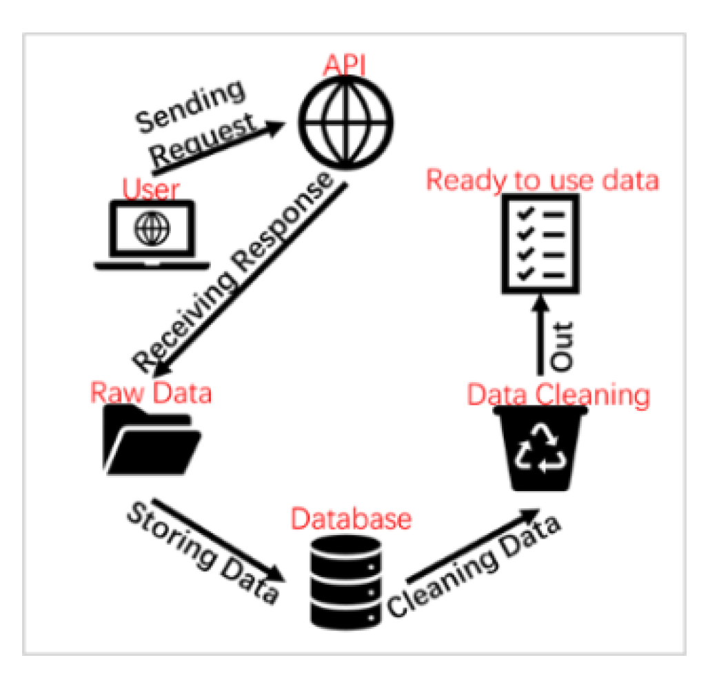
In this paper, traffic data were obtained from Brisbane City Council (BCC) via an Application Programming Interface (API). Due to the large volume of real-time traffic flow data, a traditional data processing approach (such as using hardware storage) cannot efficiently harvest, store, and analyse such big data [30]. Therefore, in this paper, we adopt a data processing procedure similar to the Real-time Traffic Information system, consisting of four parts—collecting, processing, analysing, and publishing real-time traffic data [31]. As shown in Figure 1, the data processing procedure includes four steps, which are capturing, storing, cleaning, and outputting data accordingly.
3.3. Data Sources
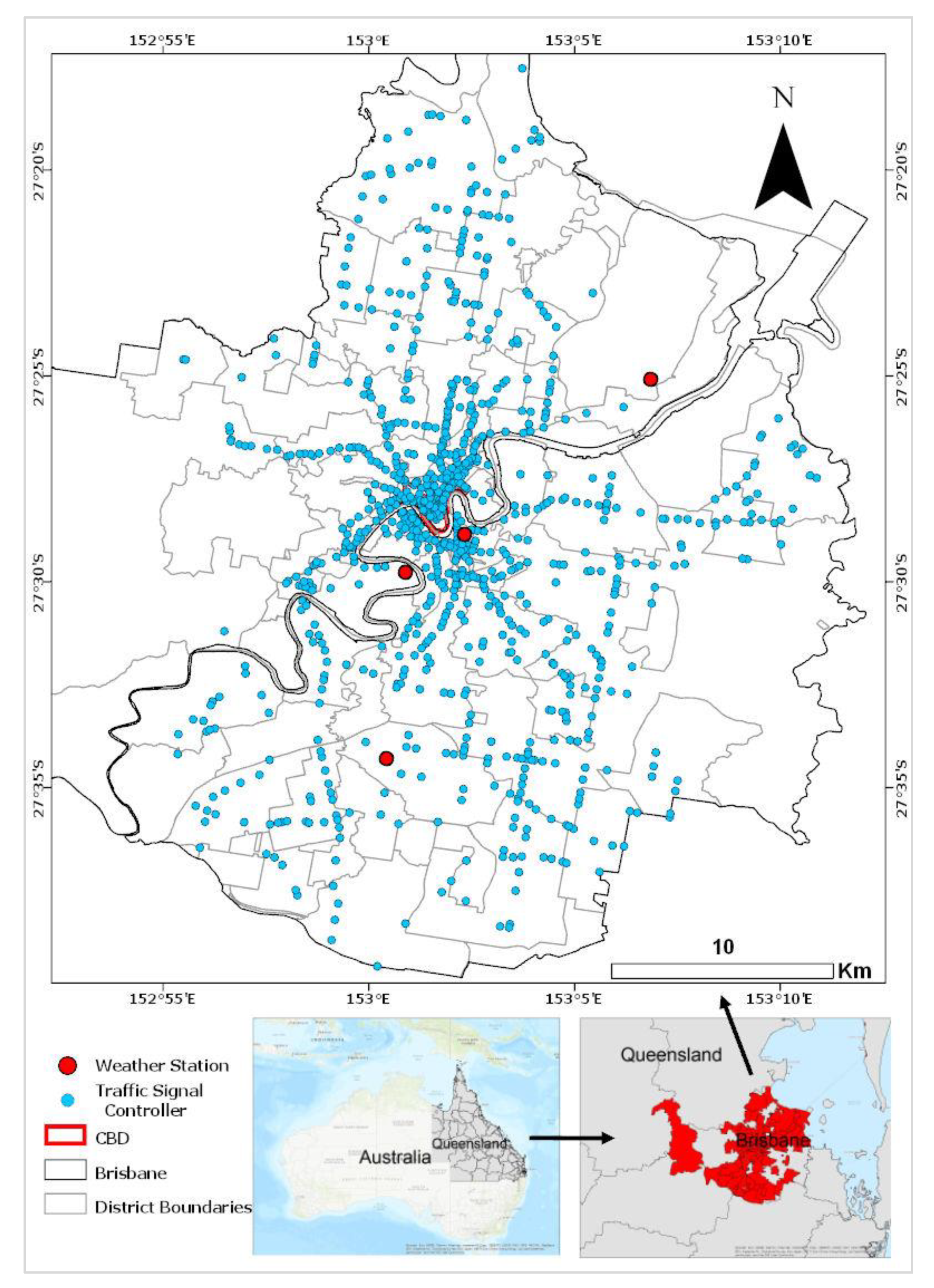
To distinguish the distribution patterns of traffic flow under different weather conditions, we selected traffic flow data from an open database of BCC [32] and weather information archived at the University of Queensland as the principal data sources, as shown in Table 1. Note that Wei et al. [33] showed the four weather stations in Brisbane (Figure 2) were highly correlated. Therefore, we can use the weather data at the University of Queensland (UQ) to represent the whole city. In total, we had access to 856 TSCs, and the weather station in UQ records 12 weather parameters, from which three parameters important for road traffic, temperature (°C), rainfall (mm) and wind speed (km/h), were selected. We obtained traffic flow data from TSC that records traffic flows every one minute and then, we aggregated the traffic flow data for every 15 min. The 15 min time resolution of traffic flow data is reasonable for our study because it can filter out random fluctuations in traffic flow rate but still capture meaningful changes [6]. The weather information at the weather station is updated every one minute, and to make the time resolutions of these two data sources consistent, we averaged the weather parameters for every 15 min. The spatial distributions of TSCs and weather stations are illustrated in Figure 2.
We collected the raw traffic flow data and weather data in Brisbane for two months (September and October 2018) and selected 12 days’ data based on data completeness [35] and the coverage of different weather conditions and day types (shown in Table 1). Note that Saturday and Sunday are regarded as two distinct day types, because travel activities on these two days are often different from each other, as suggested in the literature [26].
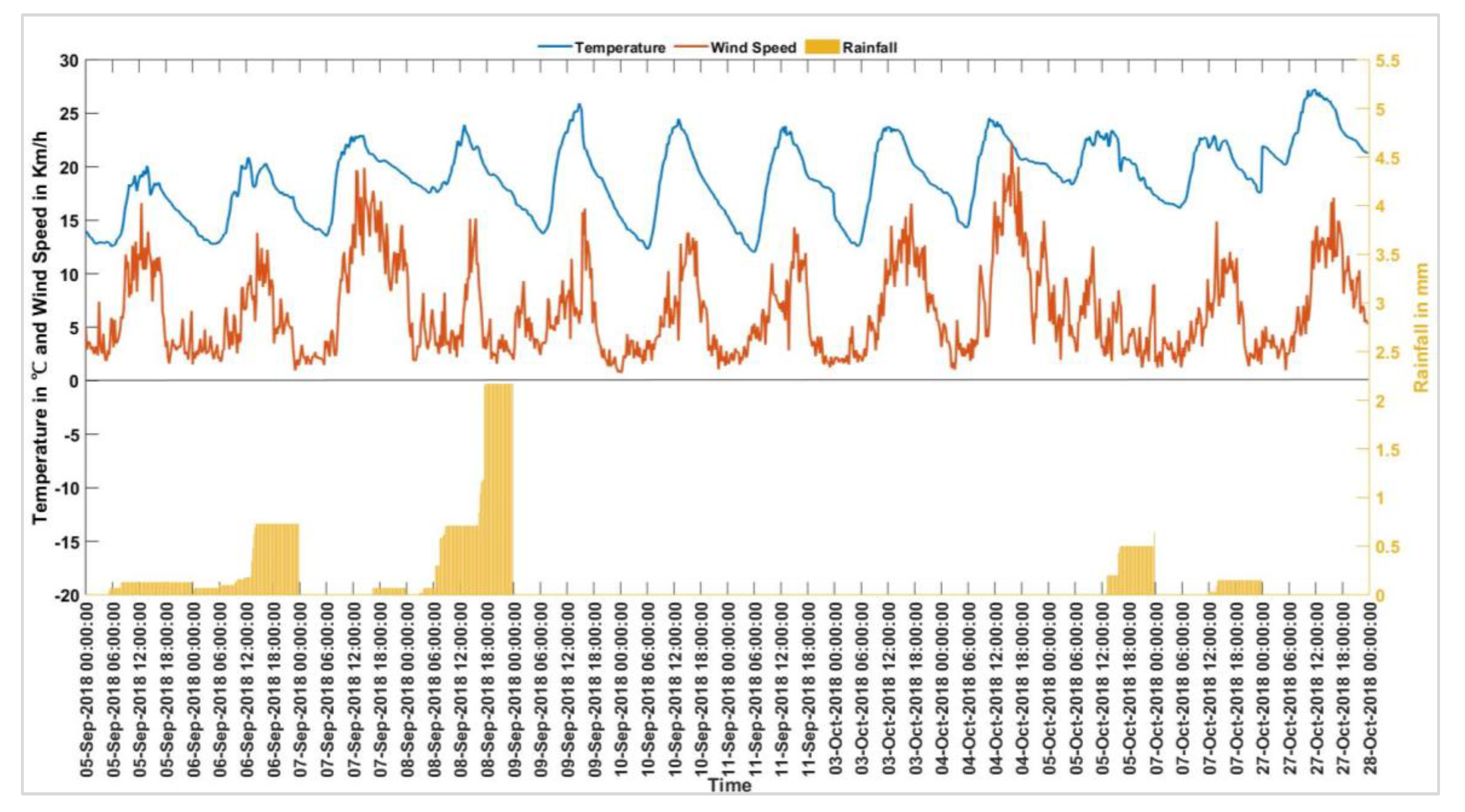
Figure 3 depicts the daily patterns of three weather parameters (temperature, wind, and rainfall). The average values of temperature and wind speed are 17.9 °C and 6.5 Km/h, respectively, on wet weekdays, while 18.6 °C and 6.7 Km/h on dry days. On the wet Saturday, the daily rainfall is 2.17 mm, with an average temperature of 19.5 °C and an average wind speed of 5.0 Km/h. On the dry Saturday, the average wind speed and temperature are 7.7 Km/h and 23.5 °C, respectively. On the dry Sunday, the average wind speed is 5.6 km/h and the average temperature is 18.7 °C.
4. Methodology
To understand weather’s impact on traffic flow qualitatively and quantitatively, more specifically, rainfall’s impact on traffic flow, we use various visualisation techniques to directly illustrate any potential weather impact on traffic flow and use statistical methods to detect the relationship between weather and traffic flow. These techniques and methods are introduced below.
4.1. Traffic Pattern Visualisation
To illustrate the influence of weather variables on the spatial-temporal distribution of traffic flow, two visualisation techniques, i.e., space-time cube and time-series clustering, are used to visualise the traffic flow patterns at each TSC under different weather conditions, as elaborated below.
- Space-Time Cube
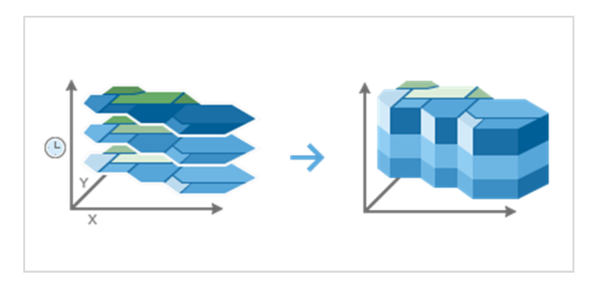
Space-time cube [36] is defined as a three-dimensional array T (T = [x, y, t]), where x, y are the location coordinates and t is the trip departure time, as shown in Figure 4. In this paper, x and y represent the coordinates of each TSC, and t is the time resolution of traffic flow data, which is 15 min by default. The value in each space-time cube is the total traffic flow within 15 min at each TSC on each day. Once a space-time cube in different weather conditions on a specific day is generated, the spatial-temporal distribution of traffic flow is extracted and visualised based on the predefined space-time cube using time-series clustering, which is introduced below.
- Time-Series Clustering
Time-series clustering [38] uses K-medoids to classify the time-series clusters in which the medoid (one particular TSC in our study) is the centre of a cluster and has the minimum dissimilarity between itself and other TSCs within the same cluster [39]. Using this method, TSCs can be classified into different clusters.
4.2. Statistical Models
To quantitatively understand weather’s impact on traffic flow, statistical models are developed to identify the relationship between inclement weather and traffic flow.
Based on the results from the two visualisation techniques introduced above, we first use traffic flow as the dependent variable and weather conditions as the independent variables to directly explore weather’s impact on traffic flow using linear regression analysis. Then, we use traffic flow time-series clusters as the dependent variable and weather conditions as the independent variables to further explore weather’s impact on the change of traffic flow trend. Since traffic flow time-series clusters are categorical, linear regression analysis is not suitable. Thus, logistic regression analysis is used, instead. Moreover, traffic flow time-series clusters are ranked, and weather’s impact on their ranking is modelled using ordered logistic regression. These statistical models are introduced below.
- Linear Regression (LR) Model
LR can model the relationship between a response variable and a set of independent variables, and has been used to model the relationship between weather and traffic flow in the literature (e.g., reference [27]). A general form of the linear regression model considered in our study is shown below,
where is the traffic flow of the th observation, is the th independent variable (e.g., daily rainfall, day of the week or TSCs categories) for the th observation, and is the regression coefficient for the th independent variable.
- Multiple Logistic Regression (MLR) Model
MLR is a statistical model that can be used to observe how the independent variables may affect the dependent variables when the dependent variables are nominal and its outcomes are more than two [40]. For possible outcomes (e.g., time-series cluster ranking in this study), when the outcome is selected as the pivot or reference, totally independent binary logistic regression models would be calculated, as illustrated below:
where is the regression coefficient for the th independent variable when the outcome is , is th independent variable (e.g., daily rainfall, day of the week or TSCs categories) of the th observation when the outcome is m.
- Ordered Logistic Regression (OLR) Model
OLR is a statistical model that can detect the impact from independent variables on the dependent variables when the dependent variables are ordinal. In this study, traffic flow time-series clusters are further ranked into three categories—low, moderate, and high. OLR is adopted to model weather’s impact on such ranking.
The equation of OLR can be defined as follows:
where is the ordinal response, is the endpoint that can set the continuous scale for , is the continuous variables (unobserved) that belong to the observed dependent variables (e.g., time-series cluster ranking in this study), , is the vector of independent variables, is the vector of coefficients, and is the error term. For c possible outcomes, totally independent binary logistic regression models would be estimated, and according to the proportional odds assumption, the coefficients of all these logistic regression models are the same [40]. In modelling ordinal dependent variables (for example, time-series cluster ranking in this study), the logit transformation is applied to the cumulative probabilities for maintaining the category order, as shown in the equation below.
A typical model for the cumulative logits is: , where = 1, …, ; c is the total number of categories; are n explanatory variables; are corresponding coefficients.
- Confusion Matrix
To comprehensively assess the performance of MLR and OLR, the confusion matrix is used. More specifically, the confusion matrix consists of True Positive, False Positive, False Negative, and True Negative, as defined below [42]:
True positive (TP): The actual and predicted cluster categories are the same for any cluster category.
False positive (FP): The actual outcome does not belong to a specific cluster category, but the predicted outcome belongs to a specific cluster category.
False negative (FN): The actual outcome belongs to a specific cluster category, but the predicted outcome does not belong to a specific cluster category.
True negative (TN): The actual and predicted outcomes do not belong to a specific cluster category.
Based on TP, FP, TN, and FN, some additional indicators can be calculated:
Sensitivity: The indicator to measure the performance of a prediction model about whether the model can predict the outcome in a specific cluster category correctly when the actual outcome belongs to that specific cluster category, which is defined as:
Specificity: The indicator to value how good the prediction model is incorrectly determining the cluster categories, and is defined as:
When interpreting the results, it is not reliable to rely on sensitivity. Both a high value of sensitivity and a high specificity are necessary for a good prediction model.
Positive Predictive Value (PPV): A ratio of the number of true positive values to the total number of positive values (TP + FP), which represents the portion of the positive values that have been predicted correctly, and is defined as:
Negative Predictive Value (NPV): A ratio of the number of true negative values to the total number of negative values (TP + FP), which represents the portion of the negative values that have been predicted correctly, and is defined as:
Positive and negative predictive values would change when the numbers of actual observations in a specific cluster category change.
Accuracy: The prediction accuracy is defined as:
5. Results
In this section, we apply the proposed methods to explore the spatial-temporal relation between traffic flow and weather conditions using the data collected in Brisbane. Two parts are presented in this section—one is the visualisation results of weather’s impact on traffic flow, and the other is the modelling results for the relationship between weather and traffic flow.
5.1. Visualisation of Traffic Flow Pattern
We first process the total traffic flows of the whole study region. We aggregate traffic flow every 15 min at multiple TSCs for each day, then determine how the traffic flow trend changes at each day across different periods. Finally, by comparing plots of weather data with traffic flow trends, the relationship between traffic flow and weather conditions is visually represented.
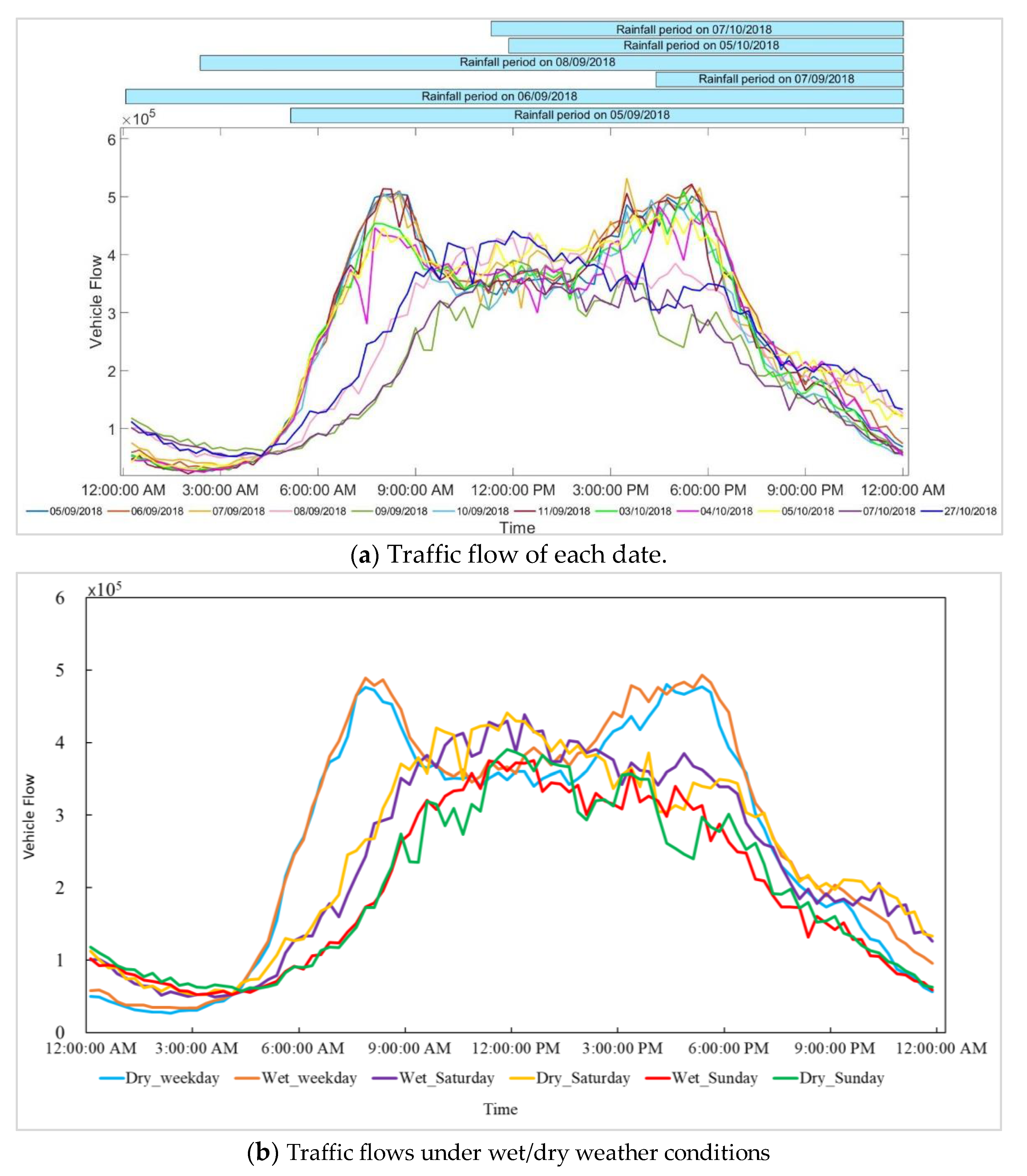
Figure 5a depicts the total aggregated traffic flow over the target days. This figure shows that generally, the traffic flow on weekday reaches peak points during the morning peak hours (around 7:30 a.m. to 8:30 a.m.) and the afternoon peak hours (around 4:30 p.m. to 5:45 p.m.), regardless of weather conditions. In addition, a similar trend can be found on Saturday and Sunday, although the peak hours of the weekends occur near noon (around 11:00 a.m. to 1:00 p.m.). However, from this figure, the trending of traffic flow on each target date can be observed, no obvious difference of traffic flow under various weather conditions can be detected. Combining with Figure 5b, we can visually identify that the aggregated weekday traffic flow in the wet weather condition is generally higher than that on the dry weekday, but no clear trend can be observed for Saturday and Sunday.
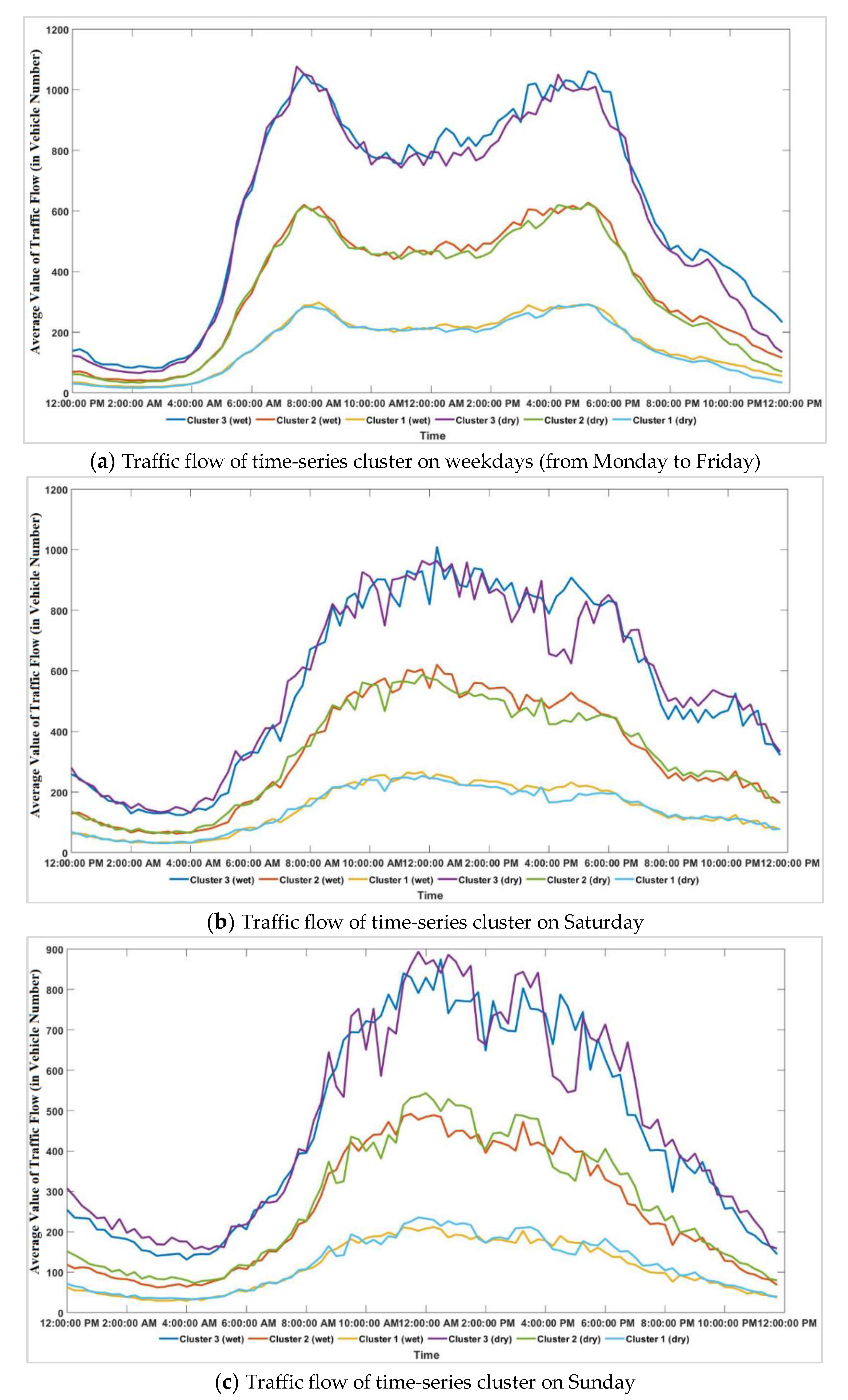
We first adopt time-series clustering to categorize all TSCs’ traffic flow in terms of the traffic amount while considering three day types. Figure 6 demonstrates the TSC traffic flow profile on different day types, which can be grouped into three clusters (traffic flow change patterns of the low traffic flow group, moderate traffic flow group, and high traffic flow group) for both wet and dry days with the similar traffic pattern. Specifically, the morning peak hours (7:30 a.m. to 8:30 a.m.) and evening peak hours (4:30 p.m. to 5:45 p.m.) on weekdays are in line with the results from the total aggregated traffic flow trends in Figure 5, while the only peak hours appear on both Saturday and Sunday. Moreover, no significant changes can be detected when visually comparing the traffic flow trend for the time-series cluster under wet and dry conditions.
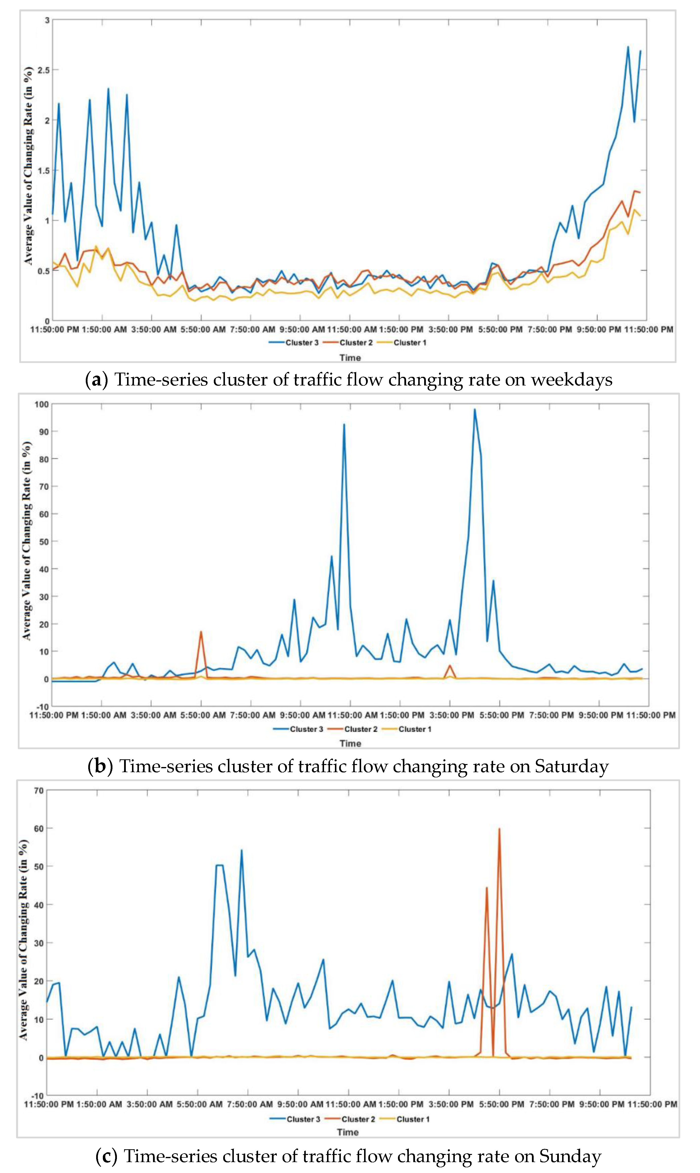
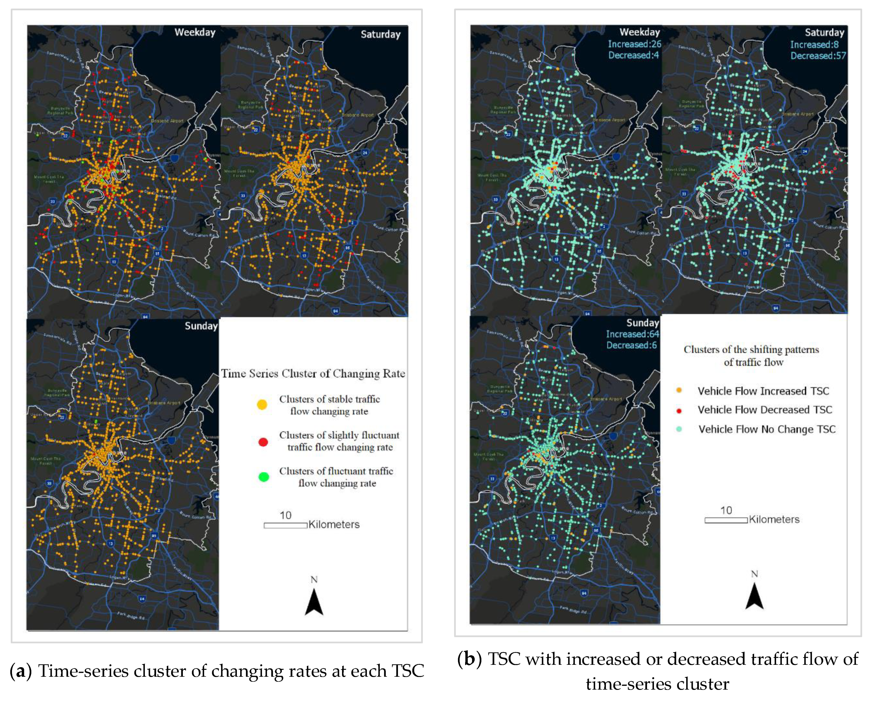
We then apply time-series clustering to further explore the changing rate (The equation for calculating the changing rate: where is the changing rate (relative to dry days), a is the traffic flow on wet days, and b is the traffic flow on dry days) of traffic flow on three day types (Figure 7). It is observed that three clusters can be classified on each day type. In particular, the higher changing rate appears at two periods on weekdays (12:00 a.m. to 5:00 a.m. and 8:00 p.m. to 12:00 p.m.), while it normally occurs on Saturday between 10 a.m. and 6 p.m., and Sunday between 6 a.m. and 8 p.m., respectively. Based on the changing rate profile of each cluster, it is reasonable to classify cluster 1 as stable, cluster 2 as slightly fluctuant, and cluster 3 as fluctuant (see Figure 7), accordingly.
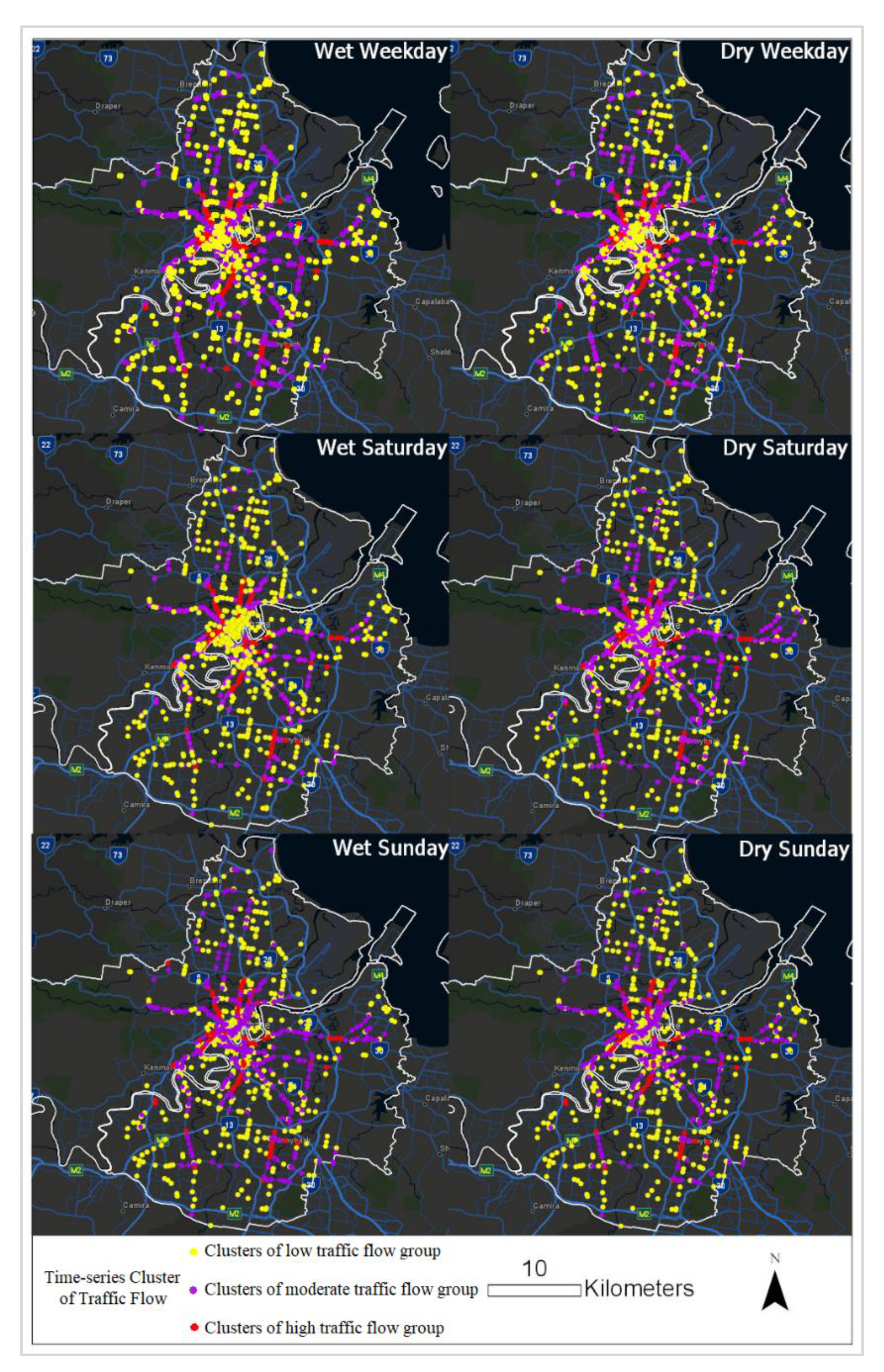
The corresponding spatial distributions of the time-series traffic flow clusters (traffic flow change patterns) are shown in Figure 8. It is found that on weekdays and Sundays, there is no significant difference in the spatial distribution of time-series clusters between the dry and wet weather conditions. On Saturday, however, in the wet weather, most TSCs in the CBD area are classified into cluster 1 (traffic flow change patterns of the low traffic flow group), while in the dry weather, most TSCs in CBD areas are labelled as cluster 2 (traffic flow change patterns of the moderate traffic flow group).
The time-series clusters of changing rates at each TSC are displayed spatially in Figure 9a, which suggests that traffic flow on weekdays fluctuates more significantly, while it is relatively stable on Sunday. By implementing a tool named Combinatorial Or [43] in ArcGIS, we further clustered the shifting patterns of traffic flow at each TSC into three clusters—Increased (TSCs shift from the low traffic flow cluster on dry days to the high traffic flow cluster on wet days), Decreased (TSCs shift from the high traffic flow cluster on dry days to the low traffic flow cluster on wet days), and No Change (TSCs belong to the same cluster class on both dry and wet days), as shown in Figure 9b. It is clear that more TSCs on Saturday have the “Decreased” shifting situation, while on Sunday, more TSCs belong to “Increased” class. In the modelling section, we use these TSCs’ classes to determine the impact of the spatial character of TSCs on traffic flows.
In summary, compared to the dry weather conditions, the traffic flow increases under wet weather on weekdays and Sunday, while declining on Saturday (see Figure 9b). In wet weather conditions, vehicles normally run slowly due to the slippery road surface, which may lead to a declining capacity of the public transport system to carry passengers. In addition, the speed awareness monitors deployed across the city [44] may also change the speed limit to slow down driving speed. On weekdays and Sundays, people have to travel for certain compulsory activities (e.g., working schedule and religious activities on Sunday mornings) despite the weather conditions, that is, the traffic demand is fixed in this situation. The possibility of taking private vehicles or commercial vehicles would be higher for passengers to avoid delay and to reduce the discomfort level caused by inclement weather. This can also be partially explained by the findings [45] that under inclement weather conditions, the travel distance would reduce, except the trips with commuting purposes, and the proportion of people choosing walking and biking would also decrease. As for on Saturday, people may choose to stay at home and some outdoor activities might be cancelled due to inclement weather, therefore, the demand for extra vehicles would reduce.
Overall, the above results from using the visualisation techniques reveal both the spatial and temporal distribution of traffic flow at each TSC considering weather impact. Next, we investigate how daily rainfall impacts traffic flow at each TSC using statistical modelling methods.
5.2. Modelling Weather’s Impact on Traffic Flow
To thoroughly investigate weather’s impact on traffic flow, we develop three levels of statistical analysis in this section: first the comprehensive level, then the location-specific level, and finally, the aggregate level, as explained below in detail. By doing so, consistent results on rainfall’s impact on traffic flow can be convincingly obtained.
5.2.1. Comprehensive Level
At this level, we develop statistical models to quantitatively investigate how traffic flow is affected by potential important factors, such as day type, weather condition (daily rainfall), and the TSC classification. Specifically, two dependent variables are considered: the total traffic flow at each TSC on each day (TOTAL_FLOW) and the classifications of time-series cluster (Cluster_ID, Cluster_ID = 1, 2, 3). Independent variables include the day type (DAY_OF_WEEK), which is classified into Weekday = 1, Saturday = 2, Sunday = 3, daily rainfall (RAIN_ACC), and the TSC classification. According to the results in Section 5.1, we can categorize TSCs in two ways (Figure 9): (1) classifying the TSCs in terms of the clusters of traffic flow changing rate at each TSC location (Stable = 1, Slightly Fluctuant = 2, Fluctuant = 3), which is denoted as TSC_CLASS_A, and (2) classifying the TSCs in terms of the changing direction of the clusters (Increased = 1, Decreased = 2, No change = 3), which is denoted as TSC_CLASS_B. We apply LR to model the total traffic flow of TSC and use MLR/OLR to model classifications of time-series cluster, respectively. To compare the models with these two different classifications of TSC, we apply the Akaike Information Criterion (AIC), which reflects the relative quality of statistical models for a given set of data. The best models using LR, MLR, and OLR are summarized in Table 2; it is noteworthy that we select 70% of the raw data as the training data to calibrate the MLR/OLR model and the remaining 30% of the raw data as the testing data to validate the model.
Table 3 illustrates the summary statistics of the variables that are adopted in the LR model (Model_2) and MLR model (Model_3)/OLR model (Model_5); the same variables are included in the MLR and OLR models. We use variance inflation factors (VIF) to detect the multicollinearity, and the results (Table 4) show that the VIF values of all the independent variables are less than 5.0, which indicates no existence of multicollinearity has been detected [10] and simultaneous involvement of these independent variables would not affect the analytic results of the models.
The values of estimated parameters of the LR model (Model_2) are listed in Table 5, which shows rainfall (RAIN_ACC) has a significant impact on the total traffic flow. When holding other factors constant, a one unit increase in rainfall (RAIN_ACC) would lead to an increase of 861 vehicles to the total traffic flow. Meanwhile, day types also have significant impacts on the total traffic flow. More specifically, the amount of total traffic flow would decline on Saturday and Sunday, when compared with weekdays. In addition, the total traffic flow would increase among the TSCs where the shifting pattern of traffic flow belongs to the “Decrease” category (TSC_CLASS_B = 2), relative to TSCs in the “Increase” category. The impact of TSC_CLASS_B = 3 (p-value > 0.05) on the total traffic flow is marginally significant.
All the parameters that used in the MLR model (Model_3) are summarized in Table 6, which shows that all the variables that are used to calculate the odds of time-series clusters being classified into traffic flow change patterns of the low traffic flow group instead of the moderate traffic flow group are statistically significant. When controlling for other factors, with a one unit increase in the rainfall (RAIN_ACC), the odds of time-series clusters being classified into traffic flow change patterns of the low traffic flow group are 26% (i.e., (exp(0.235)1) = 0.26) higher than the odds of being classified into traffic flow change patterns of the moderate traffic flow group. Meanwhile, for Saturday and Sunday, the odds of time-series clusters that can be classified into traffic flow change patterns of the low traffic flow group are 64% (i.e., (exp(0.495)1) = 0.64) and 25% (i.e., (exp(0.224)1) = 0.25) larger, respectively, than the odds of the clusters being classified into traffic flow change patterns of the moderate traffic flow group, relative to weekdays. Finally, for time-series clusters at TSCs with slightly fluctuant traffic flow changing rate (TSC_CLASS_A = 2) and time-series clusters in TSCs with large fluctuant traffic flow changing rate (TSC_CLASS_A = 3), the odds of clusters being categorized into traffic flow change patterns of the low traffic flow group are more than five (i.e., (exp(1.868)1) = 5.48) and more than nine (i.e., (exp(2.349)1) = 9.48) times greater, respectively, than the odds of the clusters being classified into traffic flow change patterns of the moderate traffic flow group, relative to the clusters in TSCs with stable traffic flow changing rate (TSC_CLASS_A = 1), which basically implies that moderate traffic flow is often stable with a small changing rate.
Table 7 summarizes the results of the OLR model (Model_5), which shows that rainfall (RAIN_ACC) has a significant impact on the category of time-series clusters (response variable). When holding other factors constant, with a one unit increase in RAIN_ACC, the odds of the time-series clusters being classified into traffic flow change patterns of the high traffic flow group (instead of the moderate or low traffic flow group) or traffic flow change patterns of the moderate traffic flow group, (instead of the low traffic flow group) would diminish by 21.2% (i.e., (exp (−0.238)1) × 100% = −21.2%). Additionally, the category of the time-series clusters is significantly impacted by day type. For Saturday and Sunday, when holding other factors constant, the odds of the time-series clusters being classified into traffic flow change patterns of the high traffic flow group (instead of the moderate or low traffic flow group) or traffic flow change patterns of the moderate traffic flow group (instead of the low traffic flow group) would decrease respectively by 38.6% (i.e., (exp(−0.487)1) × 100% = −38.6%) and 16.6% (i.e., (exp(−0.182)1) × 100% = −16.6%), relative to weekdays. Lastly, TSC classification (TSC_CLASS_A) is significantly correlated to the category of time-series clusters. More specifically, for the clusters at the TSCs that have slightly fluctuant traffic flow changing rate (TSC_CLASS_A = 2) and the clusters at the TSCs with fluctuant traffic flow changing rate (TSC_CLASS_A = 3), when holding other factors constant, the odds of the time-series clusters being categorized into traffic flow change patterns of the high traffic flow group (instead of the moderate or low traffic flow group) or traffic flow change patterns of the moderate traffic flow group (instead of the low traffic flow group) would decrease respectively by 85.6% (i.e., (exp(−1.937)1) × 100% = −85.6%) and 92.8% (i.e., (exp(−2.629)1) × 100% = −92.8%), relative to clusters in the TSCs with a stable traffic flow changing rate (TSC_CLASS_A = 1).
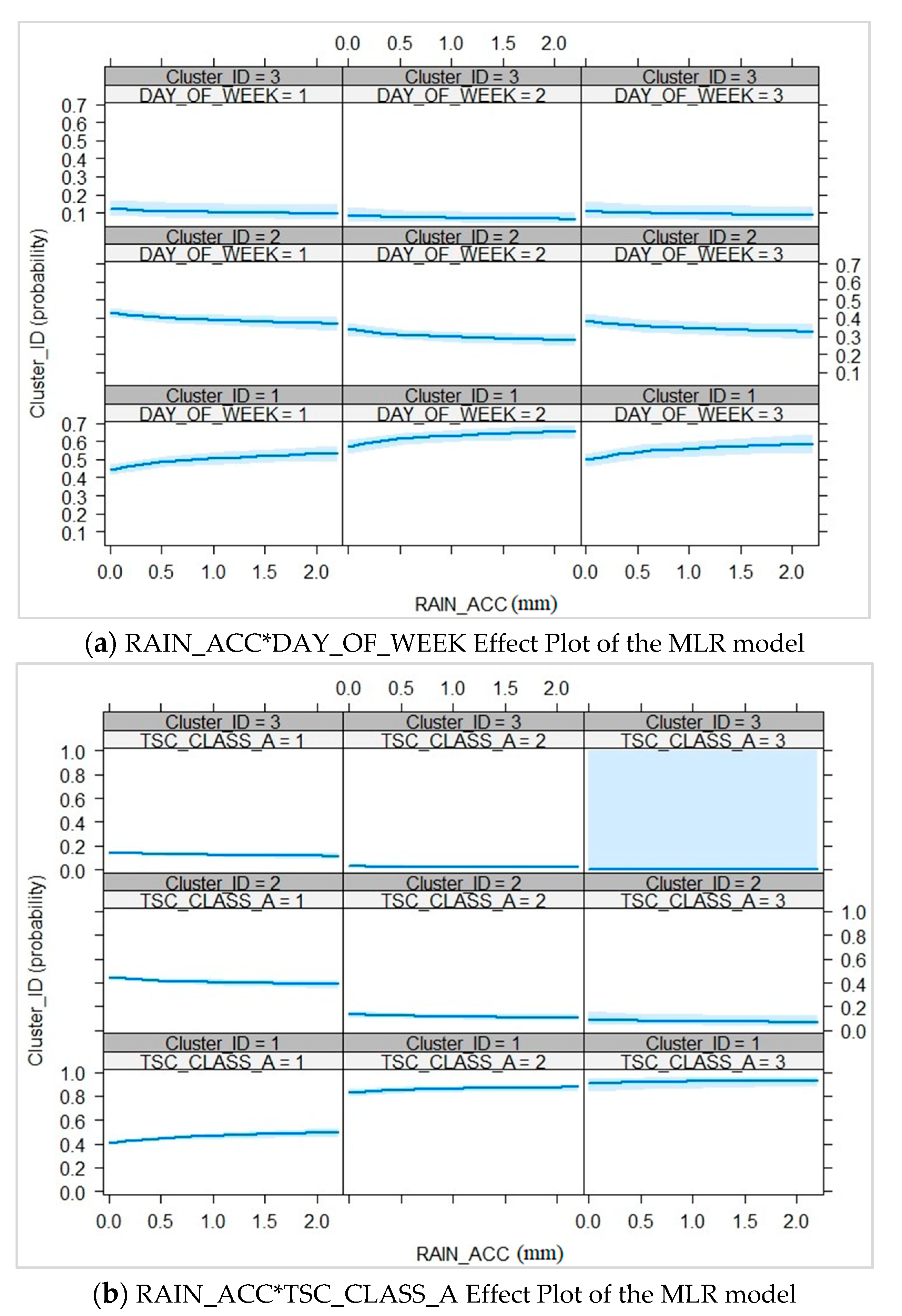
For the MLR model, from the effect plot of RAIN_ACC and DAY_OF_WEEK (Figure 10a), it is obvious that the possibilities of clusters being classified into traffic flow change patterns of the low traffic flow group are slightly higher than into the moderate traffic flow group on the dry weekdays. When the rainfall increases, the possibilities of time-series clusters being categorised into traffic flow change patterns of the low traffic flow group on three day types (weekdays, Saturday, and Sunday) would rise, while the odds of the clusters being categorised into traffic flow change patterns of the moderate and high traffic flow group would both drop. Overall, the possibility for the cluster trend to be categorised into traffic flow change patterns of the high traffic flow group is low, no matter on the dry or wet days. The similar changing patterns of possibilities happen on dry and wet Saturdays and Sundays. Among all these three days’ types, the possibility of time-series cluster being classified into traffic flow change patterns of the low traffic flow group on Saturdays (both on wet and dry) is the highest.
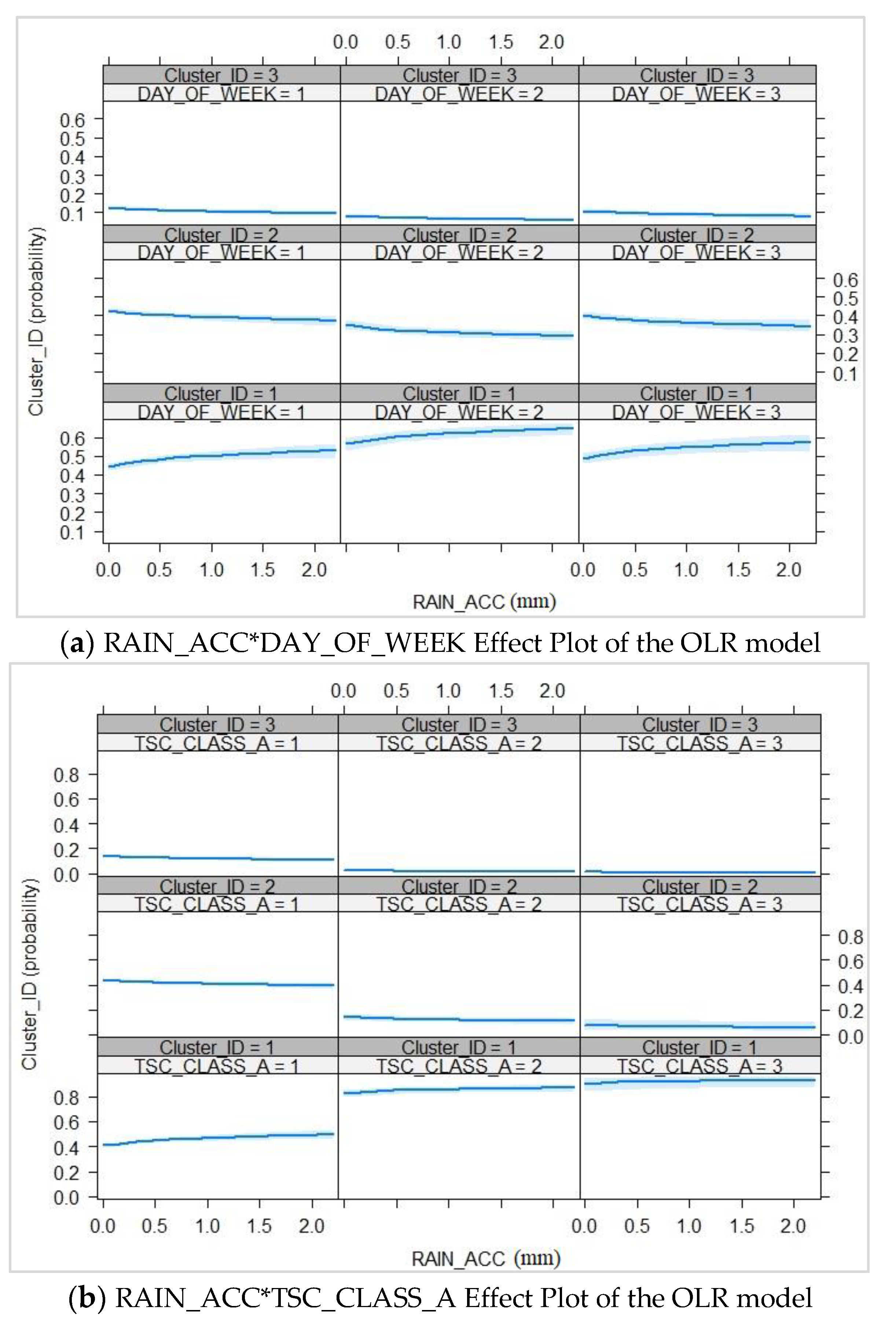
The effect plot of RAIN_ACC and TSC_CLASS_A is shown in Figure 10b. In dry weather situations, traffic flow change patterns of the low traffic flow group would have a bigger possibility to appear in the regions where the TSCs belong to TSC_CLASS_A = 3, while traffic flow change patterns of the moderate and high traffic flow group have a greater chance to show in the areas where the TSCs belong to TSC_CLASS_A = 1. When the rainfall increases, the possibility of time-series cluster being classified into traffic flow change patterns of the low traffic flow group in these three TSC_CLASS_A classes would increase, but the situations for traffic flow change patterns of the moderate and high traffic flow group are the opposite. Under inclement weather, the time-series clusters in TSC_CLASS_A = 3 have the highest odds (among three TSC_CLASS_A classes) of being classified into traffic flow change patterns of the low traffic flow group, while traffic flow change patterns of the moderate and high traffic flow group have the highest chance of being associated with TSC_CLASS_A = 1 (compared with the situations in other TSC_CLASS_A categories). Similar conclusions can be drawn from the results of the OLR model (Figure 11a,b).
Next, we cross-validate the performances of Model_3 and Model_5 by using the testing data and the confusion matrix. Table 8 summarizes the prediction indicators for MLR and OLR models. It is observed that the prediction accuracy for traffic flow change patterns of the low traffic flow group is the best among all three clusters for both MLR and OLR models. Overall, both MLR and OLR models can reasonably predict each cluster, and the prediction accuracy for each cluster is over 50%.
5.2.2. Location-Specific Level
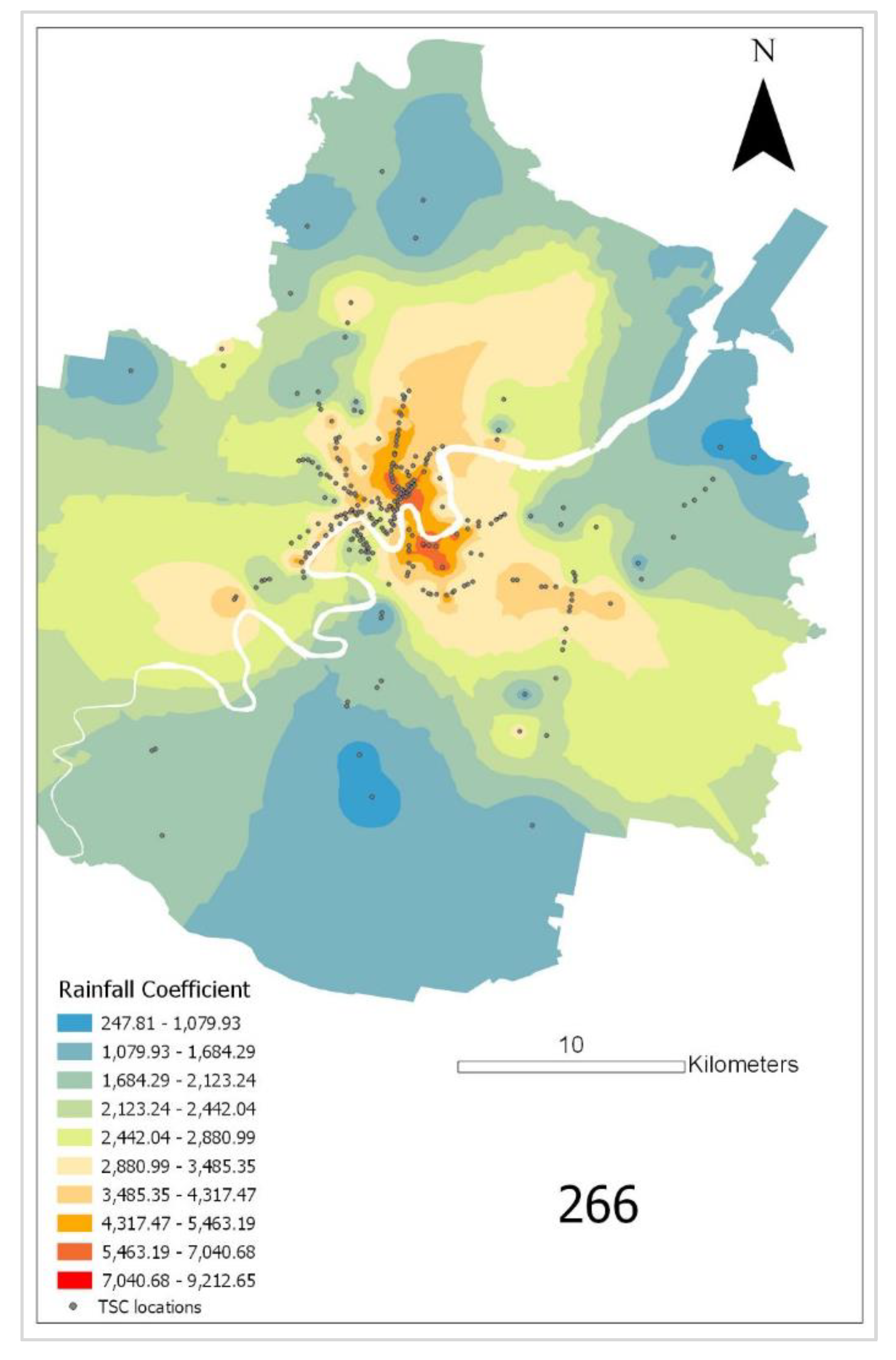
At this level, we test whether rainfall has a significant impact on traffic flow at fixed locations. From the analysis above, it is evident that TSC location can have a notable impact on the relationship between weather conditions and traffic flow. To derive more insight, we develop a linear regression model for each TSC to reveal the spatial weather impact on traffic flows. In total, 877 models are developed. Amongst these models, for 266 TSCs, rainfall appears to be a significant factor (p-value < 0.05). For these TSCs, where rainfall has a significant impact on traffic flow, a tool called inverse distance weighted in ArcGIS [26] is utilized to visualise the impact of the rainfall on traffic flow at each TSC, based on the coefficient of rainfall in the linear regression model (as depicted in Figure 12). From Figure 12, overall, these models consistently show that as the rainfall increases, traffic flow at each TSC tends to increase; moreover, the traffic flows of TSCs in the inner districts such as Kangaroo Point, Coorparoo, Fortitude Valley, and Spring Hill are more likely to be affected by the rainfall than those in the suburbs.
5.2.3. Aggregate Level
To further confirm the conclusions drawn from location-specific (TSC-controlled) analysis so far, we also modelled the impact of rainfall on traffic flow at the aggregate level across all the locations, where the dependent variable is the total traffic flow within 15 min on each day (SUM_FLOW), the independent variables are rainfall data within 15 min (RAIN_ACC_15min), and the day of data captured (DAY_OF_WEEK), respectively. The summary statistics of the variables can be identified from Table 9 and based on the total 1152 observations, we obtain the LR model (Table 10). In this model, all the variables (p < 0.05) have significant correlations with traffic flow, which is in line with the results above. Particularly, a positive impact of rainfall on the total traffic flow is also revealed, which is consistent with our conclusion drawn at location-specific level and the comprehensive level.
6. Discussion and Conclusions
By utilizing space-time cube, time-series clustering, and statistical modellings, we have qualitatively and quantitatively analysed rainfall’s impact on traffic flow spatially and temporally, using the TSC datasets in Brisbane, Australia, as a case study.
The main contribution of this study is that the spatial-temporal impact of inclement weather conditions on traffic flow has been consistently detected using the visual detections and modellings at different levels. Some findings regarding the fundamental relation among traffic flow, traffic flow change pattern, weather conditions, day types, and spatial distributions of traffic flow are concluded and summarized below. A positive impact of rainfall on the total traffic flow is also revealed, which is consistent with our conclusion drawn at location-specific level and the comprehensive level.
From the qualitative approach using spatial-temporal cube and time-series clustering, we have shown the difference of the spatial-temporal patterns of traffic flow and the distribution of traffic flow change pattern under various weather conditions on different day types. To gain more insights on the relationship between the spatial-temporal patterns of traffic flow and the rainfall, a series of statistical models have been developed.
From the quantitative approach using statistical models, rainfall’s impact on traffic flow is consistently detected from the models at three different levels. First, at the comprehensive level (i.e., all the important factors are simultaneously considered in a single model, such as day type, daily rainfall, and location), it is noticeable that rainfall, day types, and locations are all significantly correlated to traffic flow and change patterns of traffic flow. Generally, traffic flow on weekdays is the highest, while it is low on Sunday under both dry and wet weather conditions; traffic flow in wet weather normally increases compared with that in dry weather conditions; the traffic flow at the locations where the change patterns of traffic flow shift from the high traffic flow patterns on dry days to the low traffic flow patterns on wet days is higher than the traffic flow at the locations with the opposite shifting direction of traffic flow change patterns.
Meanwhile, when it comes to the traffic flow change patterns, the total traffic flows on dry days and wet days at locations are classified into three groups (dry/wet day low traffic flow group, dry/wet day moderate traffic flow group, dry/wet day high traffic flow group), respectively, the traffic flow at each location (on dry/wet days) has been categorized into one specific traffic flow group, and the related traffic flow change pattern can be detected. The classification results show that the amount of traffic flow in each classified traffic flow group on wet days is higher than the corresponding group on dry days. Furthermore, rainfall has a notable impact on traffic flow change patterns, as summarized below.
On dry days, the odds of having low traffic flow group on the locations with fluctuant changing rate of traffic flow is higher than that on all the other locations; for the dry day moderate and high traffic flow groups, they have greater possibilities of occurring at the locations with stable changing rate of traffic flow. The same patterns happen in the wet weather condition. The larger the rainfall is, the higher the odds of having low traffic flow group occurring on the locations with fluctuant changing rate of traffic flow. The rainfall would also increase the odds of Saturdays having low traffic flow group, which is in line with the implication [46] that the increased frequency of precipitation events would decrease the number of trips on specific days with leisure purposes. Additionally, when the rainfall increases, although the possibilities of having moderate and high traffic flow group on locations with stable changing rate of traffic flow would decline, they still have a greater chance of appearing on these locations compared with other locations. Overall, the results above illustrate the rainfall’s impact on the classified traffic flow group and traffic flow change pattern at each location spatially and temporally, and reveal how the traffic flow at each location changes over time on a dry/wet day.
Finally, the location-specific analysis depicts that the locations in the urban inner space, such as CBD, are more likely to be impacted by the inclement weather, and that the rainfall’s impact on traffic flow in the urban inner region is bigger than in the urban outer area. Finally, the aggregate level analysis detects the impact of rainfall on traffic flow across different locations. Specifically, the rainfall positively impacts the total traffic flow.
To summarize, we have implemented various methodologies to comprehensively analyse the impact of rainfall on traffic flow both qualitatively and quantitatively, and at three levels (i.e., comprehensive, location-specific, and aggregate). The results from our analyses consistently show that both traffic flow and traffic flow change patterns are significantly affected by the inclement weather conditions (i.e., the traffic flow would increase on wet days, especially on weekday), and that the rainfall can induce the change of traffic flow temporally (on weekdays, Saturday, and Sunday and at various periods of each day) and spatially (at different locations in the transportation network).
By recognising the spatial-temporal impacts of rainfall on traffic flow, the locations and time periods that are significantly influenced by rainfall can be identified, which can be used by planners or researchers to more accurately model the impact of rainfall on transport infrastructures. Furthermore, since our analysis shows an increase in traffic flow in wet weather, this finding can have important implications on traffic congestion and road safety. Because in wet weather, drivers usually drive more cautiously and more slowly to avoid collision due to reduced friction between the vehicle’s tires and the road surface, such behaviour means that traffic congestion is more likely to occur in wet weather.
Some limitations in this paper will be further addressed in our future work. First, this paper only considers two months’ traffic data in Brisbane. In the future, more data will be used to cover more diverse weather conditions. Moreover, public transit should be considered in future studies. Meanwhile, we have applied MLR and OLR to statistically model the spatial-temporal relation between weather conditions and traffic flow. In the future, data mining and deep learning methods could be considered.
Author Contributions
Conceptualization, Y.Q., Z.Z. and D.J.; Methodology, Y.Q., Z.Z. and D.J.; Software, Y.Q.; Writing—original draft preparation, Y.Q. and D.J.; Writing—review and editing, Z.Z.; Visualization, Y.Q.; Supervision, Z.Z. All authors have read and agreed to the published version of the manuscript.
Funding
This research received no external funding.
Conflicts of Interest
The authors declare no conflict of interest.
References
- Li, X.; Lv, Z.; Hu, J.; Zhang, B.; Yin, L.; Zhong, C.; Wang, W.; Feng, S. Traffic Management and Forecasting System Based on 3D GIS. In Proceedings of the 2015 15th IEEE/ACM International Symposium on Cluster, Cloud and Grid Computing, Shenzhen, China, 4–7 May 2015; pp. 991–998. [Google Scholar]
- Toole, J.L.; Colak, S.; Sturt, B.; Alexander, L.P.; Evsukoff, A.; González, M.C. The path most traveled: Travel demand estimation using big data resources. Transp. Res. Part C Emerg. Technol. 2015, 58, 162–177. [Google Scholar] [CrossRef]
- Tang, J.; Liu, F.; Zhang, W.; Zhang, S.; Wang, Y. Exploring dynamic property of traffic flow time-series in multi-states based on complex networks: Phase space reconstruction versus visibility graph. Phys. A 2016, 450, 635–648. [Google Scholar] [CrossRef]
- Agarwal, M.; Maze, T.H.; Souleyrette, R. Impacts of Weather on Urban Freeway Traffic Flow Characteristics and Facility Capacity. In Proceedings of the 2005 Mid-Continent Transportation Research Symposium, Ames, IA, USA, 18–19 August 2005; pp. 1–14. [Google Scholar]
- Vlahogianni, E.I.; Karlaftis, M.G. Comparing traffic flow time-series under fine and adverse weather conditions using recurrence-based complexity measures. Nonlinear Dyn. 2012, 69, 1949–1963. [Google Scholar] [CrossRef]
- Smith, B.L.; Ulmer, J.M. Freeway traffic flow rate measurement: Investigation into impact of measurement time interval. J. Transp. Eng. 2003, 129, 223–229. [Google Scholar] [CrossRef]
- Camacho, F.J.; García, A.; Belda, E. Analysis of Impact of Adverse Weather on Freeway Free-Flow Speed in Spain. Transp. Res. Rec. 2010, 2169, 150–159. [Google Scholar] [CrossRef]
- Hassan, H.M.; Abdel-Aty, M.A. Predicting reduced visibility related crashes on freeways using real-time traffic flow data. J. Saf. Res. 2013, 45, 29–36. [Google Scholar] [CrossRef]
- Ding, Y.; Li, Y.; Deng, K.; Tan, H.; Yuan, M.; Ni, L.M. Detecting and Analyzing Urban Regions with High Impact of Weather Change on Transport. IEEE Trans. Big Data 2017, 3, 126–139. [Google Scholar] [CrossRef]
- Xie, K.; Ozbay, K.; Kurkcu, A.; Yang, H. Analysis of Traffic Crashes Involving Pedestrians Using Big Data: Investigation of Contributing Factors and Identification of Hotspots. Risk Anal. 2017, 37, 1459–1476. [Google Scholar] [CrossRef]
- Li, L.; Zhu, L.; Sui, D.Z. A GIS-based Bayesian approach for analyzing spatial-temporal patterns of intra-city motor vehicle crashes. J. Transp. Geogr. 2007, 15, 274–285. [Google Scholar] [CrossRef]
- Soltani, A.; Askari, S. Exploring spatial autocorrelation of traffic crashes based on severity. Injury 2017, 48, 637–647. [Google Scholar] [CrossRef]
- Song, Y.; Miller, H.J. Exploring traffic flow databases using space-time plots and data cubes. Transportation 2012, 39, 215–234. [Google Scholar] [CrossRef]
- Zhang, H.S.; Zhang, Y.; Li, Z.H.; Hu, D.C. Spatial-Temporal Traffic Data Analysis Based on Global Data Management Using MAS. IEEE Trans. Intell. Transp. Syst. 2004, 5, 267–275. [Google Scholar] [CrossRef]
- Theofilatos, A.; Yannis, G. A review of the effect of traffic and weather characteristics on road safety. Accid. Anal. Prev. 2014, 72, 244–256. [Google Scholar] [CrossRef] [PubMed]
- Maze, T.H.; Agarwal, M.; Burchett, G. Whether weather matters to traffic demand, traffic safety, and traffic operations and flow. Transp. Res. Rec. 2006, 1948, 170–176. [Google Scholar] [CrossRef]
- Prevedouros, P.D.; Chang, K. Potential effects of wet conditions on signalized intersection LOS. J. Transp. Eng. 2005, 131, 898–903. [Google Scholar] [CrossRef] [Green Version]
- Agbolosu-Amison, S.J.; Sadek, A.W.; El Dessouki, W. Inclement weather and traffic flow at signalized intersections - Case study from northern New England. Transp. Res. Rec. 2004, 1867, 163–171. [Google Scholar] [CrossRef]
- Keay, K.; Simmonds, I. The association of rainfall and other weather variables with road traffic volume in Melbourne, Australia. Accid. Anal. Prev. 2005, 37, 109–124. [Google Scholar] [CrossRef]
- Chung, E.; Ohtani, O.; Warita, H.; Kuwahara, M.; Morita, H. Effect of rain on travel demand and traffic accidents. In Proceedings of the 8th International IEEE Conference on Intelligent Transportation Systems, Vienna, Austria, 13–16 September 2005; pp. 1080–1083. [Google Scholar]
- Unrau, D.; Andrey, J. Driver Response to Rainfall on Urban Expressways. Transp. Res. Rec. 2006, 1980, 24–30. [Google Scholar] [CrossRef]
- Jaroszweski, D.; McNamara, T. The influence of rainfall on road accidents in urban areas: A weather radar approach. Travel Behav. Soc. 2014, 1, 15–21. [Google Scholar] [CrossRef] [Green Version]
- Mashros, N.; Ben-Edigbe, J.; Hassan, S.A.; Hassan, N.A.; Yunus, N.Z.M. Impact of Rainfall Condition on Traffic Flow and Speed: A Case Study in Johor and Terengganu. J. Teknol. 2014, 70, 65–69. [Google Scholar] [CrossRef] [Green Version]
- Kamarianakis, Y.; Prastacos, P. Space–time modeling of traffic flow. Comput. Geosci. 2005, 31, 119–133. [Google Scholar] [CrossRef] [Green Version]
- Hou, T.; Mahmassani, H.S.; Alfelor, R.M.; Kim, J.; Saberi, M. Calibration of Traffic Flow Models under Adverse Weather and Application in Mesoscopic Network Simulation. Transp. Res. Rec. 2013, 2, 92–104. [Google Scholar] [CrossRef] [Green Version]
- Tao, S.; Corcoran, J.; Rowe, F.; Hickman, M. To travel or not to travel: ‘Weather’ is the question. Modelling the effect of local weather conditions on bus ridership. Transp. Res. Part C Emerg. Technol. 2018, 86, 147–167. [Google Scholar] [CrossRef]
- Datla, S.; Sharma, S. Impact of cold and snow on temporal and spatial variations of highway traffic flows. J. Transp. Geogr. 2008, 16, 358–372. [Google Scholar] [CrossRef]
- Brisbane. Available online: https://en.wikipedia.org/w/index.php?title=Brisbane&oldid=914372588 (accessed on 7 September 2019).
- Bureau of Infrastructure, Transport and Regional Economics (BITRE). Urban Public Transport: Updated Trends; Information Sheet 59; Department of Infrastructure and Regional Development of Australia: Canberra, Australia, 2014. Available online: https://www.bitre.gov.au/publications/2014/is_059 (accessed on 20 September 2019).
- Li, S.; Dragicevic, S.; Castro, F.A.; Sester, M.; Winter, S.; Coltekin, A.; Pettit, C.; Jiang, B.; Haworth, J.; Stein, A.; et al. Geospatial big data handling theory and methods: A review and research challenges. ISPRS J. Photogramm. 2016, 115, 119–133. [Google Scholar] [CrossRef] [Green Version]
- Yu, J.; Jiang, F.; Zhu, T. RTIC-C: A Big Data System for Massive Traffic Information Mining. In Proceedings of the 2013 International Conference on Cloud Computing and Big Data, Santa Clara Marriott, CA, USA, 27 June–2 July 2013; pp. 395–402. [Google Scholar]
- Traffic Management—Intersection Volume. Available online: https://www.data.brisbane.qld.gov.au/.data/dataset/traffic-data-at-intersection-api (accessed on 1 September 2018).
- Wei, M.; Liu, Y.; Sigler, T.; Liu, X.; Corcoran, J. The influence of weather conditions on adult transit ridership in the sub-tropics. Transp. Res. A Policy Pract. 2019, 125, 106–118. [Google Scholar] [CrossRef]
- City Plan 2014—Neighbourhood Plan Boundaries. Available online: https://www.data.brisbane.qld.gov.au/data/dataset/city-plan-2014-neighbourhood-plan-boundaries (accessed on 5 July 2019).
- Pipino, L.; Lee, Y.; Wang, R. Data quality assessment. Commun. ACM 2002, 45, 211–218. [Google Scholar] [CrossRef]
- Farber, S.; Fu, L. Dynamic public transit accessibility using travel time cubes: Comparing the effects of infrastructure (dis) investments over time. Comput. Environ. Urban Syst. 2017, 62, 30–40. [Google Scholar] [CrossRef] [Green Version]
- Space-Time Cube Creation. Image. 2019. Available online: https://pro.arcgis.com/en/pro-app/tool-reference/space-time-pattern-mining/createcubefromdefinedlocations.htm (accessed on 8 October 2019).
- Time-Series Clustering. Available online: https://pro.arcgis.com/en/pro-app/tool-reference/space-time-pattern-mining/time-series-clustering.htm (accessed on 20 October 2019).
- Alboukadel, K. K-Medoids in R: Algorithm and Practical Examples. 2019. Available online: https://www.datanovia.com/en/lessons/k-medoids-in-r-algorithm-and-practical-examples/#pam-algorithm (accessed on 21 October 2019).
- Zheng, Z.; Lee, J.; Saifuzzaman, M.; Sun, J. Exploring association between perceived importance of travel/traffic information and travel behavior in natural disasters: A case study of the 2011 Brisbane floods. Transp. Res. Part C Emerg. Technol. 2015, 51, 243–259. [Google Scholar] [CrossRef]
- Zheng, Z.; Liu, Z.; Liu, C.; Shiwakoti, N. Understanding public response to a congestion charge: A random effects ordered logit approach. Transp. Res. A Policy Pract. 2014, 70, 117–134. [Google Scholar] [CrossRef] [Green Version]
- Sun, J.; Zheng, Z.; Sun, J. Stability analysis methods and their applicability to car-following models in conventional and connected environments. Transp. Res. B Methodol. 2018, 109, 212–237. [Google Scholar] [CrossRef]
- Combinatorial Or. Available online: https://pro.arcgis.com/en/pro-app/tool-reference/spatial-analyst/combinatorial-or.htm (accessed on 21 October 2019).
- Speed Awareness Monitors-Drive Slow for SAM. Available online: https://www.brisbane.qld.gov.au/traffic-and-transport/roads-infrastructure-and-bikeways/current-road-and-intersection-projects/speedawareness-monitors (accessed on 5 July 2020).
- Aaheim, H.A.; Hauge, K.E. Impacts of climate change on travel habits: A national assessment based on individual choices. CICERO Rep. 2005, 7, 1–38. [Google Scholar]
- Koetse, M.L.; Rietveld, P. The impact of climate change and weather on transport: An overview of empirical findings. Transp. Res. D Transp. Environ. 2009, 14, 205–221. [Google Scholar] [CrossRef]
Figure 1.
The process of generating ready-to-use data.

Figure 2.
The study site covers the whole city of Brisbane; the areas with red outline represent the central business district (CBD) region [34] and the whole city of Brisbane has been divided into 89 regions.
Figure 2.
The study site covers the whole city of Brisbane; the areas with red outline represent the central business district (CBD) region [34] and the whole city of Brisbane has been divided into 89 regions.

Figure 3.
Daily patterns of three weather parameters: temperature, wind, and rainfall.

Figure 4.
Space-time cube based on a defined location [37].
Figure 4.
Space-time cube based on a defined location [37].

Figure 5.
Various traffic flow conditions.

Figure 6.
Traffic flow of time-series cluster on various days.

Figure 7.
Time-series cluster of traffic flow changing rate on various days.

Figure 8.
Time-series cluster distribution.

Figure 9.
Two ways for categorizing TSCs.

Figure 10.
Variable Effect Plot of the MLR model.

Figure 11.
Variable Effect Plot of the OLR model.

Figure 12.
The effect of rainfall.


Table 1.
Description of the data for determining weather’s impact on traffic flow in Brisbane.
| Dataset | Data Description | Date | Data Source | |
|---|---|---|---|---|
| Traffic flow data | Recorded time TSC (Traffic Signal Controller) ID Traffic flow in each lane (4 lanes) | September 2018–October 2018 | Brisbane City Council: (https://www.data.brisbane.qld.gov.au/data/dataset/traffic-data-at-intersection-api) | |
| Weather data | Temperature (°C) Rainfall (mm) Wind speed (km/h) | September 2018–October 2018 | University of Queensland Weather Stations: (http://ww2.sees.uq.edu.au/uqweather/archive/AWS_archive/) | |
| Weather Situation (Wet/Dry) | Weekday/Weekend | Day | Date | |
| Wet | Weekday | Wednesday | 5 September 2018 | |
| Thursday | 6 September 2018 | |||
| Friday | 7 September 2018 | |||
| Friday | 5 October 2018 | |||
| Weekend | Saturday | 8 September 2018 | ||
| Sunday | 7 October 2018 | |||
| Dry | Weekday | Monday | 10 September 2018 | |
| Tuesday | 11 September 2018 | |||
| Wednesday | 3 October 2018 | |||
| Thursday | 4 October 2018 | |||
| Weekend | Sunday | 9 September 2018 | ||
| Saturday | 27 October 2018 | |||
Table 2.
Summary of models.
| Category | Model | No. of Observation | AIC | df |
|---|---|---|---|---|
| Linear Regression model | Model_1 (with TSC_CLASS_A) | 10,406 | 22,8779.40 | 7 |
| Model_2 (with TSC_CLASS_B) | 10,406 | 22,8766.70 | 7 | |
| * Model_2 has smaller AIC value, which means Model_2 is better. | ||||
| Multiple Logistic Regression model | Model_3 (with TSC_CLASS_A) | 10,648 | 19,862.29 | 10 |
| Model_4 (with TSC_CLASS_B) | 10,648 | 20,700.38 | 12 | |
| * Model_3 has smaller AIC value, which means Model_3 is better. | ||||
| Ordered Logistic Regression model | Model_5 (with TSC_CLASS_A) | 10,648 | 19,849.88 | 7 |
| Model_6 (with TSC_CLASS_B) | 10,648 | 20,742.59 | 7 | |
| * Model_5 has smaller AIC value, which means Model_5 is better. | ||||
* means the better models of using LR, MLR, and OLR.
Table 3.
Summary statistics.
| Model | Variable | Min | Max | Mean/% | SD |
|---|---|---|---|---|---|
| Model_2 (n = 10,406) | TOTAL_FLOW | 629 | 89,188 | 26,404 | 14,635.37 |
| DAY_OF_WEEK (Weekday = 1; Saturday = 2; Sunday = 3) | 1 | 3 | Weekday = 67.12% Saturday = 16.32% Sunday = 16.57% | ||
| TSC_CLASS_B (Increased = 1; Decreased = 2; No change = 3) | 1 | 3 | Increased = 3.48% Decreased = 1.69% No change = 94.83% | ||
| RAIN_ACC (mm) | 0.00 | 2.17 | 0.32 | 0.60 | |
| Model_3/Model_5 (n = 10,648) | Cluster_ID (Low traffic flow = 1; Moderate traffic flow = 2; High traffic flow =3) | 1 | 3 | Low traffic flow = 47.36% Moderate traffic flow = 40.24% High traffic flow =12.40% | |
| TSC_CLASS_A (Stable = 1; Slightly Fluctuant = 2; Fluctuant = 3) | 1 | 3 | Stable = 88.39% Slightly Fluctuant = 10.07% Fluctuant = 1.54% | ||
| DAY_OF_WEEK (Weekday = 1; Saturday = 2; Sunday = 3) | 1 | 3 | Weekday = 66.94% Saturday = 15.97% Sunday = 17.08% | ||
| RAIN_ACC (mm) | 0.00 | 2.17 | 0.31 | 0.59 |
Table 4.
Variance Inflation Factors (VIF) For Multicollinearity Detection.
| Model | Variable | VIF |
|---|---|---|
| Model_2 | DAY_OF_WEEK | 1.23 |
| TSC_CLASS_B | 1.05 | |
| RAIN_ACC | 1.17 | |
| Model_3/Model_5 | DAY_OF_WEEK | 1.39 |
| TSC_CLASS_A | 2.30 | |
| RAIN_ACC | 1.42 |
Table 5.
Estimated parameters for Model_2 of the LR model.
| Overall Goodness-of-Fit Log Likelihood = −11,4376.4; Significance Level < 0.01; AIC = 22,8766.7 | ||||
|---|---|---|---|---|
| Variable | Estimated Value | Standard Error | t_value | Pr |
| Intercept | 26,349.5 | 785.7 | 33.537 | <0.001 |
| RAIN_ACC | 861 | 339.9 | 2.533 | 0.0113 |
| DAY_OF_WEEK = 2 | −3193.7 | 420.7 | −7.592 | <0.001 |
| DAY_OF_WEEK = 3 | −7149.6 | 392.4 | −18.221 | <0.001 |
| TSC_CLASS_B = 2 | 5767.1 | 1345.1 | 4.287 | <0.001 |
| TSC_CLASS_B = 3 | 1443.6 | 780.2 | 1.850 | 0.0643 |
Note: TSC_CLASS_B = 1 and DAY_OF_WEEK = 1 are selected as reference categories, respectively.
Table 6.
Estimated parameters for Model_3 of the MLR model.
| Overall Goodness-of-Fit Log Likelihood = −6910.3; Significance Level < 0.01; AIC = 19,862.29 | ||||
|---|---|---|---|---|
| Variable | Estimated Value | Standard Error | t_value | Pr |
| 1: Intercept | −0.210 | 0.038 | −5.486 | <0.001 |
| 3: Intercept | −1.111 | 0.054 | −20.751 | <0.001 |
| 1: RAIN_ACC | 0.235 | 0.063 | 3.758 | <0.001 |
| 3: RAIN_ACC | −0.064 | 0.098 | −0.656 | 0.512 |
| 1: DAY_OF_WEEK = 2 | 0.495 | 0.077 | 6.466 | <0.001 |
| 3: DAY_OF_WEEK = 2 | −0.098 | 0.121 | −0.811 | 0.417 |
| 1: DAY_OF_WEEK = 3 | 0.224 | 0.070 | 3.201 | 0.001 |
| 3: DAY_OF_WEEK = 3 | 0.027 | 0.099 | 0.268 | 0.789 |
| 1: TSC_CLASS_A = 2 | 1.868 | 0.108 | 17.257 | <0.001 |
| 3: TSC_CLASS_A = 2 | −0.432 | 0.234 | −1.849 | 0.064 |
| 1: TSC_CLASS_A = 3 | 2.349 | 0.306 | 7.676 | <0.001 |
| 3: TSC_CLASS_A = 3 | −16.447 | 1889.594 | −0.009 | 0.993 |
Note: (i) For the response variable, Cluster_ID = 2 is selected as the reference category, while for the independent variables, TSC_CLASS_A = 1 and DAY_OF_WEEK = 1 are selected as reference categories, respectively; (ii) 1: Intercept, 1: RAIN_ACC, 1: DAY_OF_WEEK = 2, 1: DAY_OF_WEEK = 3, 1: TSC_CLASS_A = 2, 1: TSC_CLASS_A = 3 are the parameters that are used to calculate the odds of time-series cluster (response variable) being classified into Cluster_ID = 1; 3: Intercept, 3: RAIN_ACC, 3: DAY_OF_WEEK = 2, 3: DAY_OF_WEEK = 3, 3: TSC_CLASS_A = 2, 3: TSC_CLASS_A = 3 are the parameters that are used to calculate the odds of time-series cluster (response variable) being classified into Cluster_ID = 3.
Table 7.
Estimated parameters for Model_5 of the OLR model.
| Overall Goodness-of-Fit Log Likelihood = −6915.155; Significance Level < 0.01; AIC = 19,849.88 | ||||
|---|---|---|---|---|
| Variable | Estimated Value | Standard Error | t_value | Pr |
| RAIN_ACC | −0.238 | 0.056 | −4.254 | <0.001 |
| DAY_OF_WEEK = 2 | −0.487 | 0.069 | −7.066 | <0.001 |
| DAY_OF_WEEK = 3 | −0.182 | 0.062 | −2.954 | 0.003 |
| TSC_CLASS_A = 2 | −1.937 | 0.100 | −19.431 | <0.001 |
| TSC_CLASS_A = 3 | −2.629 | 0.305 | −8.611 | <0.001 |
| 1|2 | −0.476 | 0.035 | −13.670 | <0.001 |
| 2|3 | 1.651 | 0.042 | 39.549 | <0.001 |
Note: TSC_CLASS_A = 1 and DAY_OF_WEEK = 1 are selected as reference categories, respectively.
Table 8.
Summary of prediction performance of the MLR and OLR model.
| MLR model performance (Model_3) | |||||
| Cluster_ID | Sensitivity (%) | Specificity (%) | PPV (%) | NPV (%) | Accuracy (%) |
| 1 | 46.49 | 74.64 | 60.76 | 62.29 | 60.57 |
| 2 | 72.81 | 40.69 | 46.98 | 67.46 | 56.75 |
| 3 | 0 | 100 | NaN | 87.70 | 50.00 |
| OLR model performance (Model_5) | |||||
| Cluster_ID | Sensitivity (%) | Specificity (%) | PPV (%) | NPV (%) | Accuracy (%) |
| 1 | 38.80 | 84.50 | 67.89 | 62.05 | 61.65 |
| 2 | 82.83 | 32.66 | 47.03 | 72.49 | 57.74 |
| 3 | 0 | 100 | NaN | 87.70 | 50.00 |
Table 9.
Summary statistics (n = 1152).
| Variable | Min | Max | Mean/% | SD |
|---|---|---|---|---|
| SUM_FLOW | 22,172 | 531,976 | 253,111 | 148,766.80 |
| RAIN_ACC_15min (mm) | 0.00 | 2.17 | 0.14 | 0.37 |
| DAY_OF_WEEK (Weekday = 1; Saturday = 2; Sunday = 3) | 1 | 3 | Weekday = 66.67%; Saturday = 16.67%; Sunday = 16.67% |
Table 10.
Estimated parameters for aggregate level LR model.
| Overall Goodness-of-Fit Log Likelihood = −15,322.35; Significance Level < 0.01; AIC = 30,654.7 | ||||
|---|---|---|---|---|
| Variable | Estimated Value | Standard Error | t_value | Pr |
| Intercept | 258,525 | 5622 | 45.985 | < 0.001 |
| RAIN_ACC_15min | 72,460 | 13,828 | 5.240 | <0.001 |
| DAY_OF_WEEK = 2 | −44,527 | 12,217 | −3.645 | <0.001 |
| DAY_OF_WEEK = 3 | −67,290 | 11,718 | −5.743 | <0.001 |
Note: For the independent variable, DAY_OF_WEEK = 1 is selected as the reference category.
© 2020 by the authors. Licensee MDPI, Basel, Switzerland. This article is an open access article distributed under the terms and conditions of the Creative Commons Attribution (CC BY) license (http://creativecommons.org/licenses/by/4.0/).
Share and Cite
MDPI and ACS Style
Qi, Y.; Zheng, Z.; Jia, D. Exploring the Spatial-Temporal Relationship between Rainfall and Traffic Flow: A Case Study of Brisbane, Australia. Sustainability 2020, 12, 5596. https://0-doi-org.brum.beds.ac.uk/10.3390/su12145596
AMA Style
Qi Y, Zheng Z, Jia D. Exploring the Spatial-Temporal Relationship between Rainfall and Traffic Flow: A Case Study of Brisbane, Australia. Sustainability. 2020; 12(14):5596. https://0-doi-org.brum.beds.ac.uk/10.3390/su12145596
Chicago/Turabian StyleQi, Yanmin, Zuduo Zheng, and Dongyao Jia. 2020. "Exploring the Spatial-Temporal Relationship between Rainfall and Traffic Flow: A Case Study of Brisbane, Australia" Sustainability 12, no. 14: 5596. https://0-doi-org.brum.beds.ac.uk/10.3390/su12145596
Note that from the first issue of 2016, this journal uses article numbers instead of page numbers. See further details here.