Article

Sustainable Viticulture: First Determination of the Environmental Footprint of Grapes

by
Vassilis Litskas
1,2,3,*,†,
Athanasia Mandoulaki
1,
Ioannis N. Vogiatzakis
2,
Nikolaos Tzortzakis
1 and
Menelaos Stavrinides
1,*
1
Department of Agricultural Sciences, Biotechnology and Food Science, Cyprus University of Technology, 30 Arch. Kyprianos Str., 3036 Limassol, Cyprus
2
School of Pure and Applied Sciences, Open University of Cyprus, 33, Yiannou Kranidioti Avenue, 2220 Latsia, Cyprus
3
Sustainability Metrics, Valtetsiou 4, 2416 Nicosia, Cyprus
*
Authors to whom correspondence should be addressed.
http://www.sustainabilitycy.com/.
Sustainability 2020, 12(21), 8812; https://0-doi-org.brum.beds.ac.uk/10.3390/su12218812
Submission received: 13 September 2020 / Revised: 14 October 2020 / Accepted: 20 October 2020 / Published: 23 October 2020
(This article belongs to the Special Issue Waste Strategies Development in the Framework of Circular Economy)

Abstract

:
We present for the first time the environmental footprint (EF) of grapes following the methodology proposed by the EU and life cycle assessment (LCA). We used data from three different production systems, conventional high- or low-input and organic from vineyards on the Mediterranean island of Cyprus. The life cycle inventory (LCI) data were retrieved from the recently released AGRIBALYSE database, and the EF was determined with the Open LCA software. The system boundary was from “cradle to winery door” and the functional unit was 1 ton of grapes delivered to the winery. Organic grape production had the lowest values for most of the 16 EF impact categories. Machinery, fuel, and sulfur production and use were identified as EF hotspots for organic grapes. Fertilizer production and use were identified as EF hotspots for high-input grape production. The EF impact category values for low-input grapes showed similarities with organic production. Future research needs to enrich the LCI databases with data more applicable to the methods and inputs applied in Mediterranean agriculture.

1. Introduction

The European Commission proposed methods for determining the product environmental footprint and organization environmental footprint as a common way of measuring environmental performance [1]. The EU proposal aimed at providing a unified approach for environmental benchmarking of products, as the several choices, methods, and initiatives that are available may be confusing to both companies and consumers. In 2013, the communication from the Commission Building the Single Market for Green Products (COM/2013/196) established the product- and organization environmental footprint (PEF and OEF, or more generally EF). The common methods of how to measure the life cycle environmental performances for the EF were first defined in the EU Recommendation 2013/179/EU.
From 2013 to 2018, the EF pilot phase took place, which involved a number of products and companies, testing and improving the PEF and OEF methodology (see http://ec.europa.eu/environment/eussd/smgp/ef_pilots.htm). The pilot approach resulted in the Product Environmental Footprint Category Rules (PEFCRs), which describe the method and datasets to be used for determining the EF. Consequently, the 2020 “Circular Economy Action Plan” foresees that companies will have to substantiate their environmental claims using PEF and OEF methods [1]. Wine was one of the products selected in the pilot phase and, consequently, the methods and datasets used to calculate the EF of grapes and wine are now becoming available.
The EF approach aspires to provide an assessment of the most important environmental consequences. It is a multicriteria indicator taking into consideration several impacts on the environment, in addition to the carbon (CF) and the water (WF) footprints, which are the most popular indicators used to assess the environmental performance of products [2]. The EF includes a range of environmental impact indicators related to climate change, ecotoxicity, resources use, public health issues, and environmental degradation (e.g., carbon footprint, energy use, potential for causing respiratory problems to humans, eutrophication, ozone depletion). The most widely acceptable method to obtain the EF is life cycle assessment (LCA), which includes the entire supply chain and the impacts to the environment that are generated from the production [2,3]. Martinez et al. [2] published recently an informative review on the protocols followed for EF determination.
The EF of agricultural products as proposed by the EU approach is not very well studied. Due to the fact that climate change is a topic of active interest, researchers have been focusing on the determination of the CF or global warming potential (GWP) under different management systems for crops that contribute substantially to GHG emissions (e.g., rice) [4]. Organic vs. conventional agriculture are often being compared, using different environmental impact indicators and LCA [5] or indicators representing the water–food–energy nexus (e.g., water footprint, energy intensity) [6]. In the case of wine, LCA has been applied to determine several indicators, with the most popular being water and carbon footprints [7,8,9]. Other wine studies have reported additional indicators, such as eutrophication potential and ozone depletion based on LCA [10,11]. For grapes, published works covered the CF and WF (e.g., comparison of different varieties and management systems) [9,12].
The recently released EF methodology proposes a more inclusive approach through the application of LCA from “cradle to grave” to estimate 16 impact categories and provides a holistic approach for reporting the environmental impact of products and organizations. The EF approach leads to better information for the decision makers as it provides a more complete picture for environmental performance. For example, shifting from conventional to organic agriculture could reduce fertilizer use, leading to eutrophication mitigation, but could increase fuel use, which favors photochemical ozone formation and contributes to GHG emissions and respiratory problems [13,14]. Therefore, obtaining the EF indicators allows for informed decision making based on a more complete analysis of the potential environmental impacts of agricultural production. In addition, LCA and EF could be used for spatial planning [15] and ecosystem services-related research [16]. Although there are publications where LCA was applied for the environmental impact assessment of agricultural products [6,17,18], few works used the recently developed PEF approach. Soode-Schimonsky et al. [19] applied the PEF methodology to determine the environmental impacts of various strawberry production systems in Germany and Estonia. In the research, polytunnel or conventional systems had lower environmental impact than greenhouse or organic (open field) cultivation, respectively. PEF has been also studied for olive oil [20], during the PEFCR pilot for the product, to provide a benchmark for further research. This research highlighted the complexity of such studies (mainly due to the different agricultural systems and farming techniques). For viticulture, the study of the environmental impact of Sagrantino and Grechetto grapes for vinegar production in Italy got closer to the PEF philosophy [9]. In this research, carbon footprint, ecological footprint, water footprint, acidification, eutrophication, ozone layer depletion, and photochemical oxidation were used as impact categories. According to our knowledge, the PEF of grapes following the PEFCR methodology has not been assessed.
Recently, many free datasets for EF determination were released (e.g., AGRIBALYSE https://nexus.openlca.org/database/Agribalyse or JRC EF database—see https://eplca.jrc.ec.europa.eu/LCDN/contactListEF.xhtml), while open access tools for LCA are being developed (e.g., Open LCA; http://www.openlca.org/). This will facilitate the common use of data and methodology for the determination of the EF for agricultural products (at least in Europe) and encourage their use from organizations that produce them (e.g., a winery). AGRIBALYSE contains representative processes and life cycle inventory (LCI) data for grape production, which are tailored for the French viticulture. Although it may be easy to obtain data for inputs use in a certain country (e.g., type of fertilizers and amounts), processes related to the production (e.g., machinery production) are not freely available. AGRIBALYSE, as well as other EF-related databases, come to cover this gap. AGRIBALYSE provides open access and contains all the processes and flows required to model agricultural products’ EF.
Yet, estimating the EF based on data from AGRIBALYSE leads to a degree of uncertainty. For instance, the processes for fertilizer production/use in Cyprus or elsewhere might not be identical to that in France or different types of inputs/products might be used in the two countries. However, many of the data are applicable to other EU countries (e.g., pesticides, fertilizers, fuel, a wide range of machinery), making AGRIBALYSE valuable for a first estimation of the EF of products from “cradle to grave”.
Viticulture and winemaking are important for the EU economy. The EU holds a 62.9% share of the global wine production [21], followed by the USA, Argentina, and Australia. Wine production in the EU averaged 16 billion liters (L) (data for the period 2014–2020) with 50% of the wine consumed locally, another 28% transported in the intra-Union market, and the remaining 22% exported globally. The area under vines in the EU is approx. 3 million ha and the wine trade balance was about 12 billion euros in 2018 [21]. As in most Mediterranean countries, viticulture and winemaking are essential for the economy and rural development in Cyprus [22,23]. Most of the vineyards on the island are located in high nature value farmland (HNVf) areas, i.e., agricultural areas important for the conservation of species and habitats of EU importance [22]. The wine production in Cyprus is estimated to be 11–13 million L [24]. Climate change and vineyard abandonment are considered as long term threats for viticulture on the island [25,26].
The aim of this study was to estimate, for the first time, the EF of grapes following the PEFCR methodology, using Cyprus as a study system. The specific objectives of the current work were to: (1) use the flows related to agricultural production from the AGRIBALYSE database and the EF methodology to report the impact categories required for the PEFCR methodology for grapes, and (2) identify data gaps related to the determination of the EF for grape production in Cyprus and elsewhere.

2. Materials and Methods

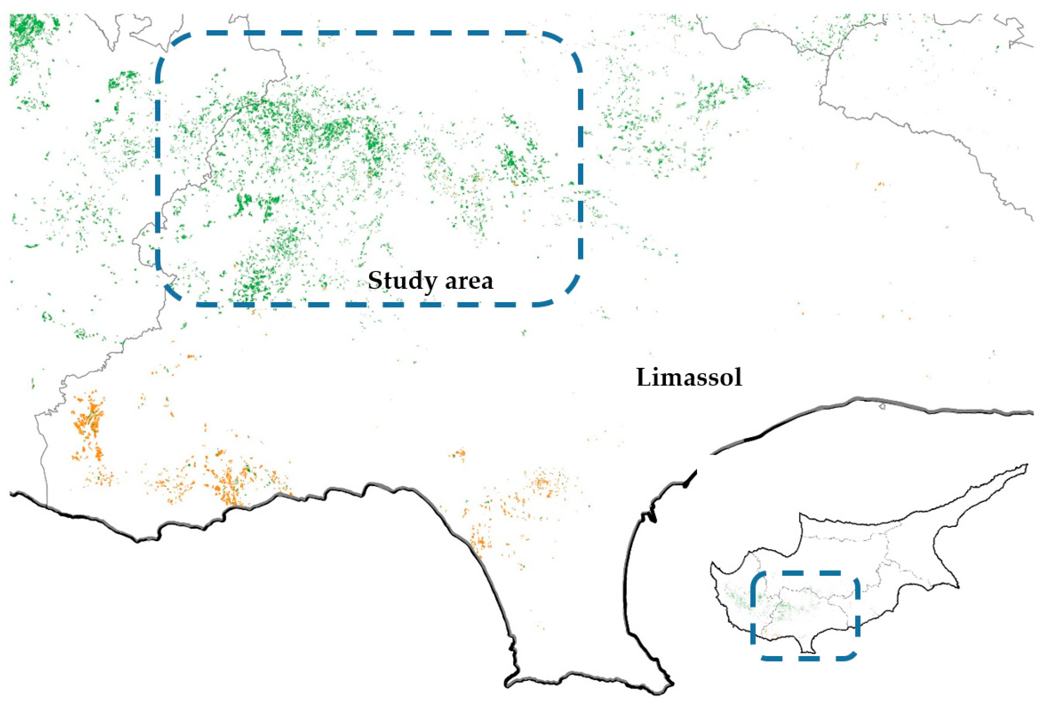
2.1. Study Area and Wineries for Data Collection

Wine grapes in Cyprus cover 5313 ha yielding 20,508 tons of grapes annually [23]. About 60% of this area is planted with the indigenous grape varieties Xynisteri (white) and Mavro (red). The current work focused on the EF of the Xynisteri variety, which is used for the production of white wine and most importantly for the mixing with Mavro for the production of the sweet dessert wine Commandaria (protected designation of origin). Commandaria’s production methods remain essentially unchanged since 800 BCE. Xynisteri, as an indigenous variety, is well adapted to the soil and climatic conditions of Cyprus. In comparison to introduced varieties it requires less inputs (e.g., pesticides, fertilizers) for grape production [12]. Typically, most of the Xynisteri vineyards are non-irrigated.
There are currently close to 70 wineries on the island, of which 63 are SMEs (Cyprus Winemakers Association, personal communication). An initial survey was carried out in six SME wineries, and three were selected who received their grapes from vineyards under production practices considered the most representative of viticulture on the island: high-input, low-input, and organic. Winery 1 (W1) uses high amounts of fertilizers and synthetic pesticides, representative of professional agriculture, W2 follows organic production practices, while W3 uses low quantities of synthetic fertilizers but not synthetic pesticides, representing the practice of many part-time farmers residing on mountainous areas. The typical annual wine production of the three wineries (not only Xynisteri) is 40,000 for W1, 80,000 for W2, and 120,000 (0.75 L) bottles for W3.
The vineyards supplying the three wineries with grapes were located in the district of Limassol, Cyprus (Figure 1). The soils in the area are Calcaric cambisols and Calcaric regosols [27]. The mean average monthly temperature range in the area is 10–28 °C and the mean annual rainfall is 600 mm. The mean annual wind speed in the area is 4–6 m/s (at 10 m above ground). Winery 1 (W1) uses on a yearly basis 15 tons of Xynisteri grapes (mean of 2017–2019), cultivated in a 2.5 ha area; Winery 2 (W2) 25 tons of grapes from 5 ha; Winery 3 (W3) 40 tons of grapes from 6.5 ha.
The wineries apply the same management practices to the vineyards from which they receive their grapes. The bush–vine training system (goblet—trellis-free) is used for all three vineyards (W1–3). The grape production methods were recorded following interviews with the winery owners and professionals (e.g., vine growers, agronomists, winemakers). Data collected for grape production, included: (1) fertilizer and (2) pesticides used (products and active ingredients) and their application rate, (3) fuel use (in machinery and for transportation), (4) machinery used (for soil cultivation; application of pesticides, manure, and fertilizers; pruning; vineyard establishment; and uprooting) (5) grape production (kg/ha), (6) pruning mass and management, and (7) distance and vehicle used for transportation of grapes to the winery.
For each viticultural practice, a list of inputs was obtained (e.g., W1 uses 20 kg of N/year). Inputs were standardized to the production of 1 ton of grapes (Tables 1–3).
Based on the input amount and type, the wineries were classified as conventional high-input (W1), organic (W2—apply practices in accordance with organic production rules), and conventional low-input (W3). The main distinction between W1 and W3 was the higher use of fertilizers in W1 than W3 (four times higher in W1) and the use of synthetic pesticides in W1 but not W3 (Tables 1 and 3). Fertilizers are hotspots for environmental impacts in viticulture [12]. The practices followed in W3 are considered representative of the effort from many of the vine growers in the study area to reduce their inputs, mainly for financial reasons.
For each of the management practices presented above, the data related to production flows and processes (e.g., machinery, pesticides, fertilizers) were obtained from AGRIBALYSE v3.0 database. AGRIBALYSE is the French LCI database for the agriculture and food sector. Version 3.0, published in 2020, contains LCIs for 2500 agricultural and food products. AGRIBALYSE is also recommended for use by the wine PEFCR [28].

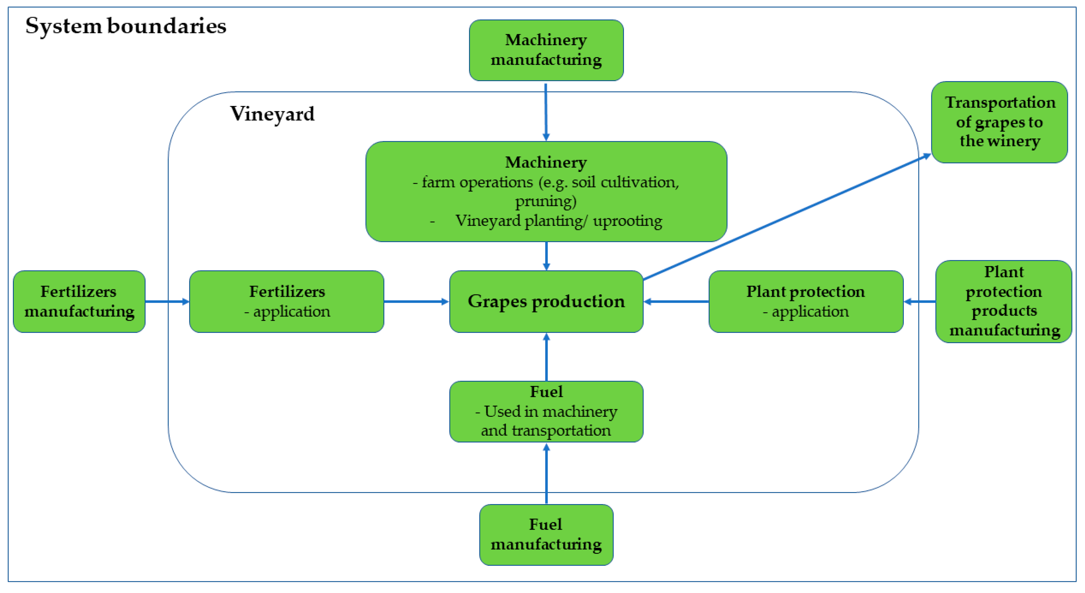
2.2. Life Cycle Assessment

Life cycle assessment was performed for the determination of the EF for Xynisteri variety grapes. Xynisteri grape production was modelled as a process in Open LCA and the system boundaries were from materials production (e.g., fertilizers, pesticides, machinery) to vineyard end of life (Figure 2). Transportation of the product to the winery was also included in the model. The functional unit was 1 ton (1000 kg) of Xynisteri grapes delivered to the winery gate. The LCI (inputs and outputs) for the three grape production methods and the modelling approach (e.g., flows codes) are provided in Supplementary Materials (Annexes I–III), as extracted from the OpenLCA.

2.3. Environmental Footprint

The EF method was followed for the impact assessment. The following (total 16) impact assessment categories were reported for full PEF estimation of the Xynisteri grapes, from cradle to grave [29]:
(1)
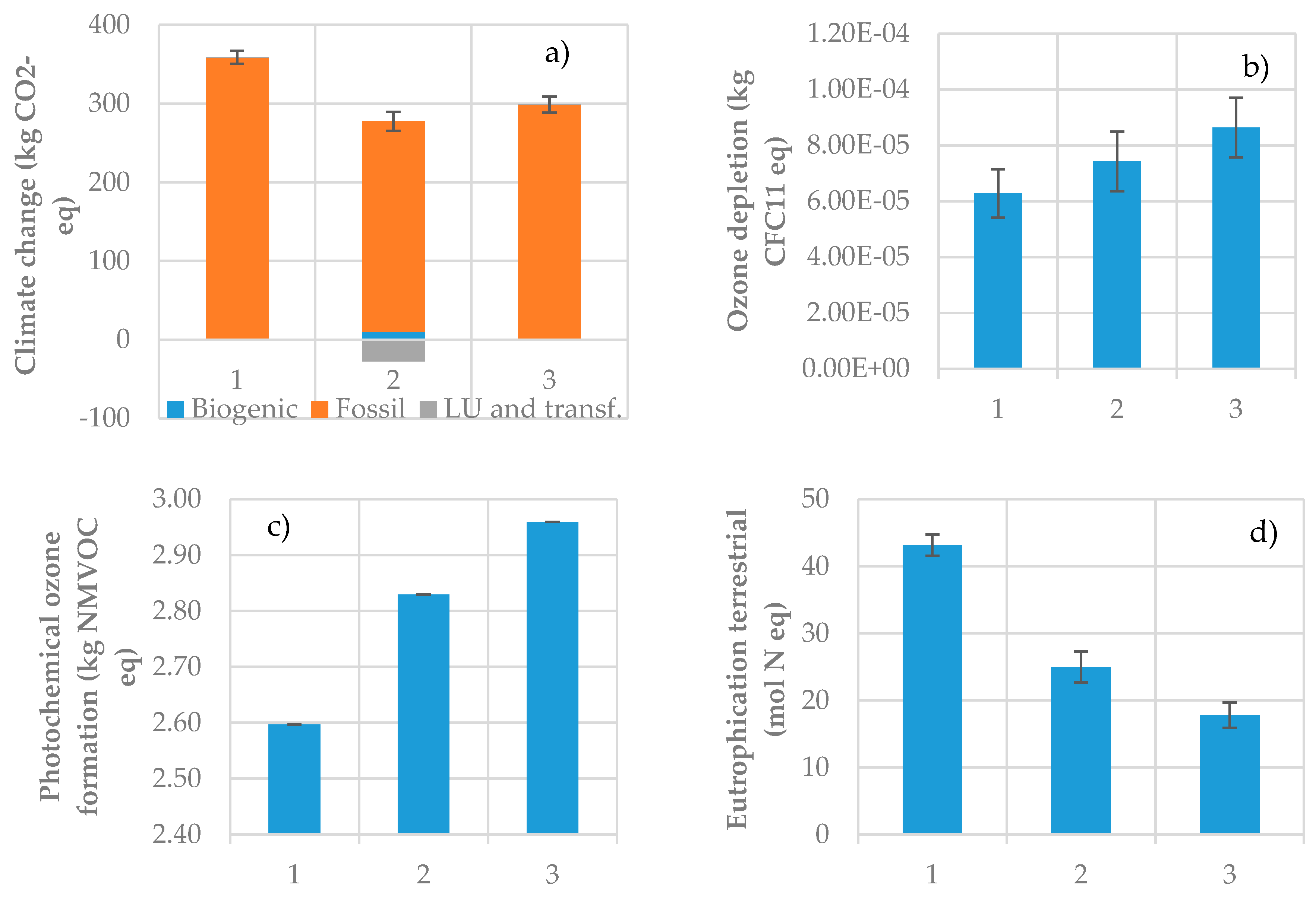
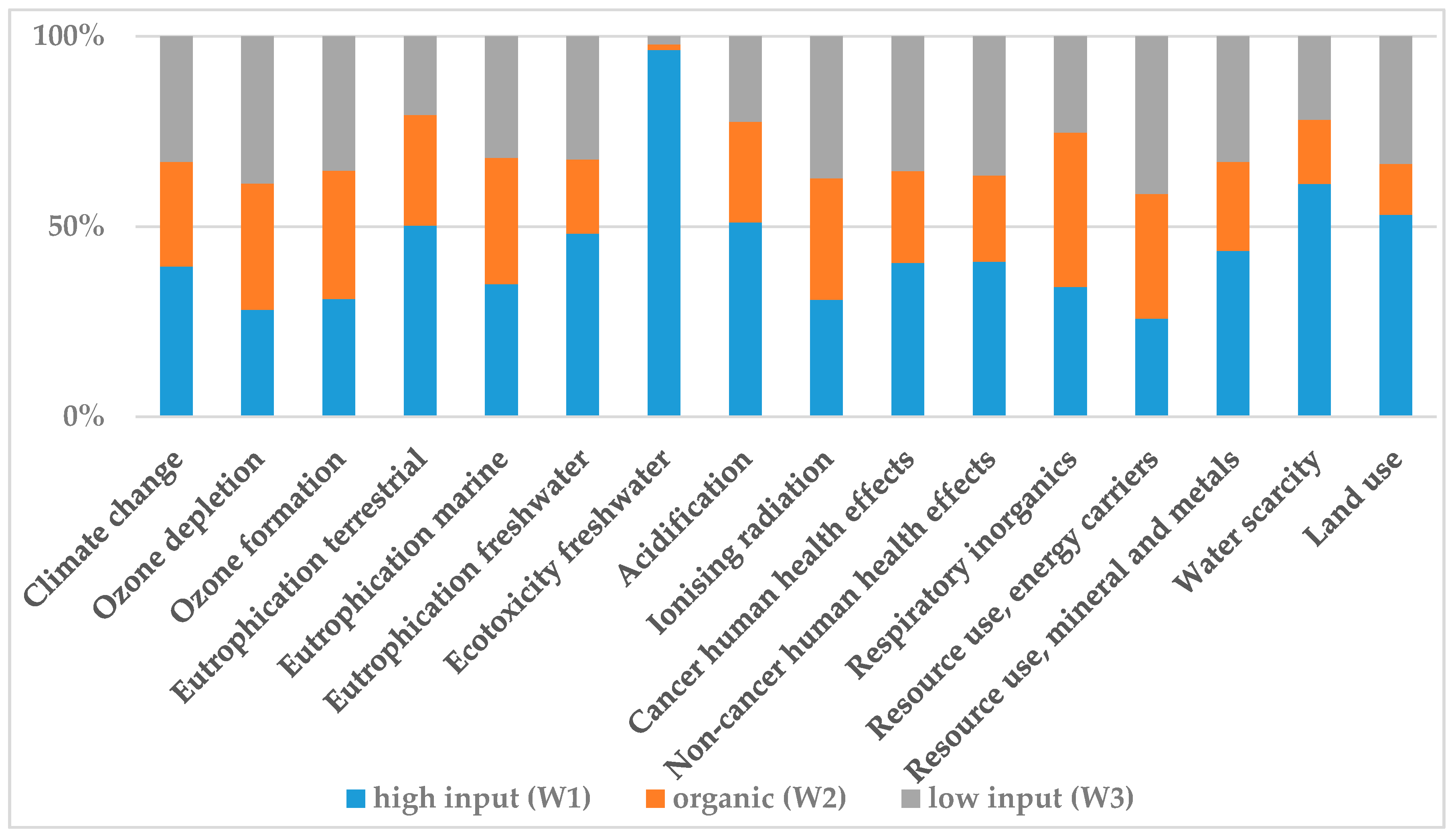
Climate change (kg CO2 eq): (a) fossil, (b) biogenic, (c) land use and transformation. Expresses radiative forcing as global warming potential (GWP100).
(2)
Ozone depletion potential (ODP) (kg CFC11 eq). Calculates the destructive effects on the stratospheric ozone layer over a time horizon of 100 years.
(3)
Photochemical ozone formation (kg NMVOC eq). Expression of the potential contribution to photochemical ozone formation.
(4)
Eutrophication terrestrial (mol N eq). Gives the N load to the terrestrial environment.
(5)
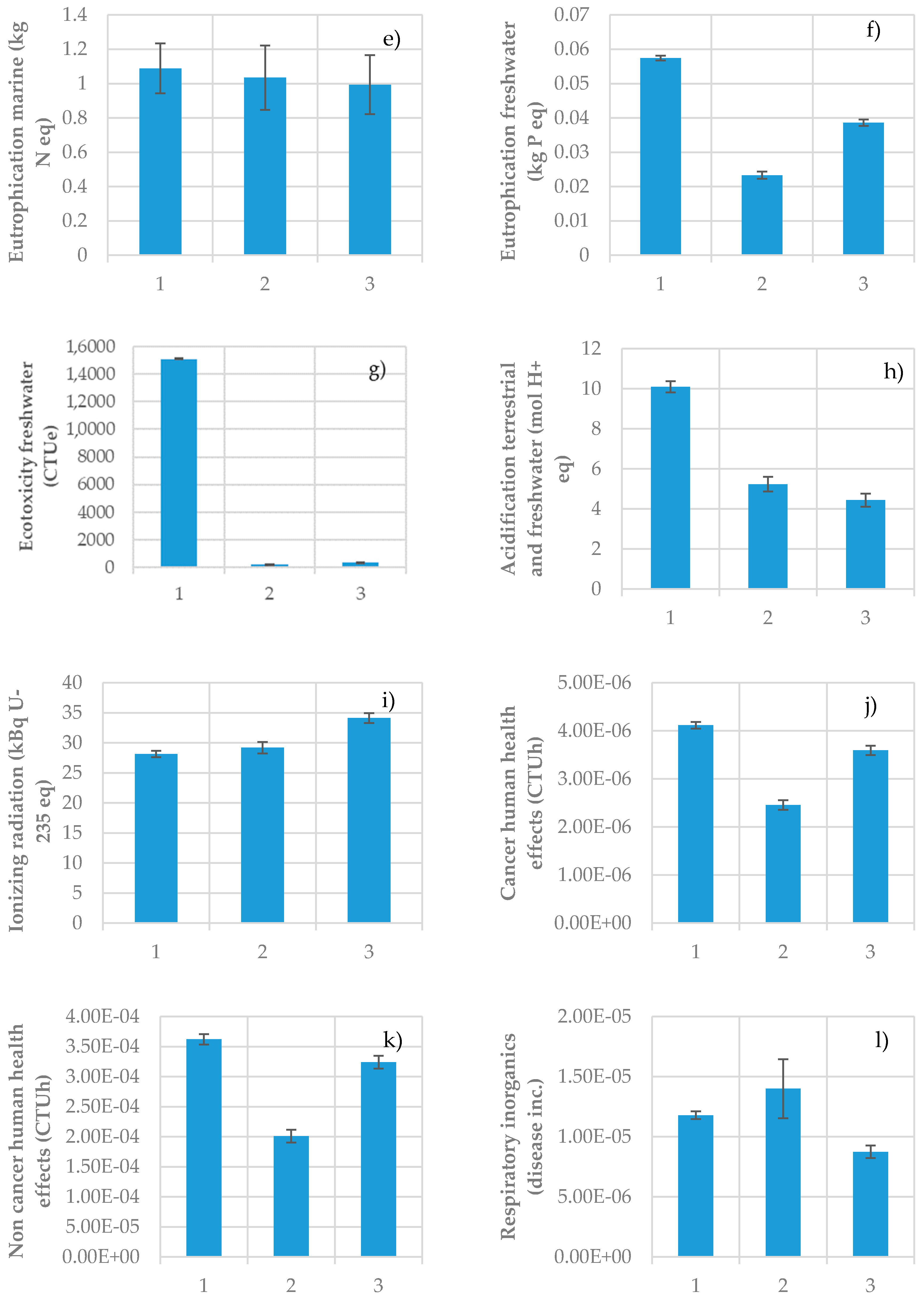
Eutrophication marine (kg N eq). Expression of the degree to which the surplus of nutrients reaches the marine end compartment (nitrogen considered as a limiting factor in marine water).
(6)
Eutrophication freshwater (kg P eq). Expression of the degree to which the emitted nutrients reach the freshwater end compartment (phosphorus considered as a limiting factor in freshwater).
(7)
Ecotoxicity freshwater (comparative toxic unit for ecosystems; CTUe). Expresses an estimate of the potentially affected fraction (PAF) of species integrated over time and volume per unit mass of a chemical emitted (PAF × m3 × year/kg of chemical emitted).
(8)
Acidification terrestrial and freshwater (mol H+ eq). Quantifies the acidifying substances deposition.
(9)
Ionizing radiation (kBq U-235 eq). Quantification of the impact of ionizing radiation on the population, in comparison to Uranium 235.
(10)
Cancer (comparative toxic unit for humans; CTUh);
(11)
Noncancer human health effects (CTUh). CTUh in (10) and (11) expresses the estimated increase in morbidity in the total human population per unit mass of a chemical emitted (cases per kilogram).
(12)
Respiratory inorganics. Expresses disease incidence due to kg of PM2.5 emitted.
(13)
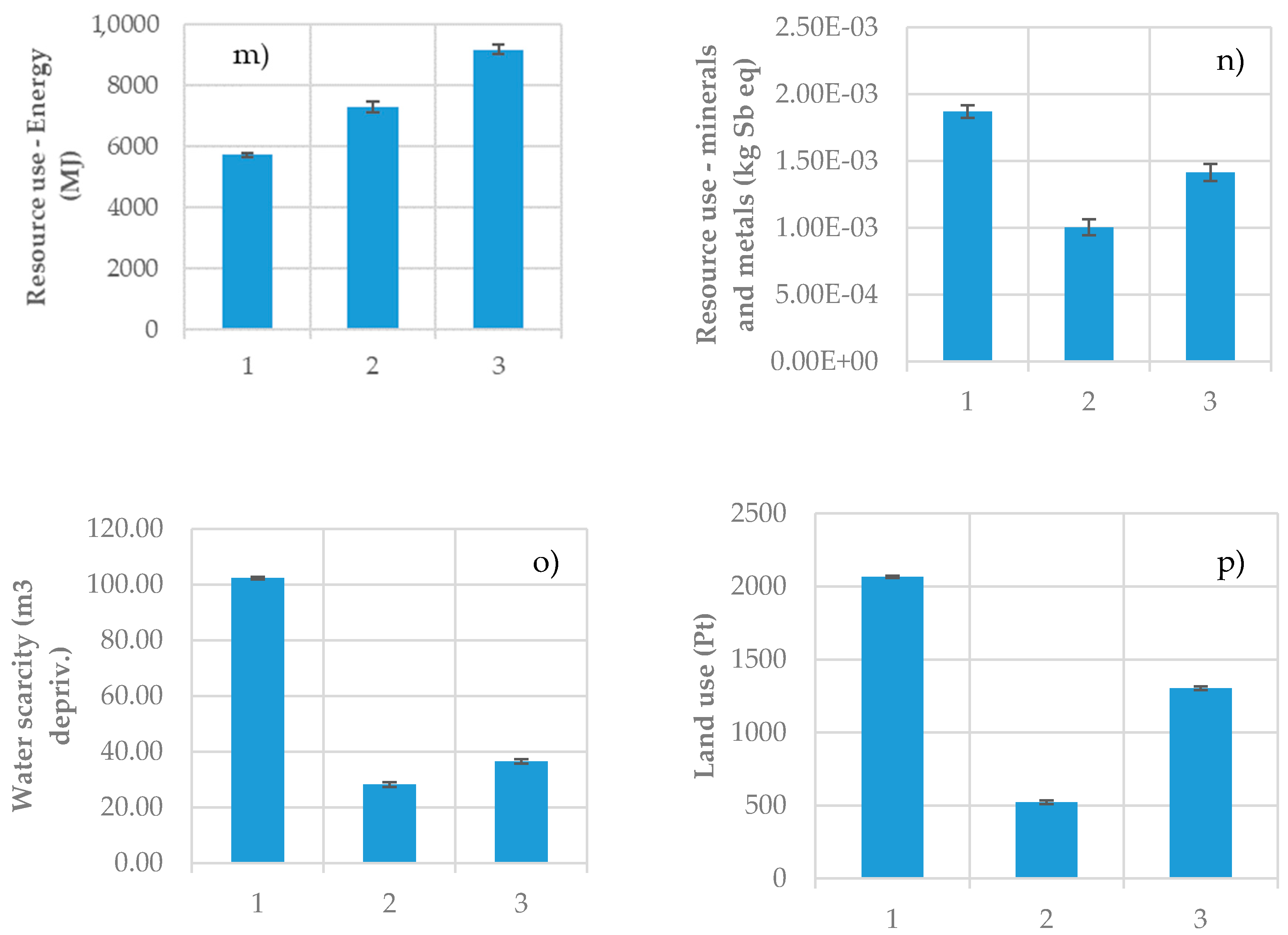
Resource use—energy carriers (MJ). Abiotic resource depletion for fossil fuels.
(14)
Resource use—minerals and metals (kg Sb eq); Abiotic resource depletion for mineral and metal resources.
(15)
Water scarcity (m3; user deprivation potential). Relative available water remaining (AWARE) per area in a watershed.
(16)
Land use. Soil quality index (indicators: erosion resistance, mechanical filtration, groundwater regeneration, biotic production); expressed in points per unit of inventory flow (Pt/m2a) [30]
More details for the methodology used for the estimation of these indicators are presented in Table A1 (Appendix A) and in PEFCR-related documents [28,29]. For each of the impact categories, the hotspots (% of the highest contribution in the total value, e.g., 23% of the total kg CO2 eq in the climate change category are attributed to diesel consumption in the vineyard) were determined for the 3 management systems studied.
C sequestration (climate change land use and transformation) due to CO2 uptake from the plants was calculated to be zero. The amount of C stored during the lifetime of the vines (30 years) was assumed to be removed from the system with vineyard destruction, as wood and roots are typically used as biomass for heating purposes (burned). Soil respiration and C stocks in the soils were not considered in the LCA.
The N2O and NH3 emissions due to the use of synthetic and organic fertilizers were accounted, as recommended in wine PEFCR [28]. Accordingly, 0.0057 kg N2O/kg N fertilizer [31] and 0.12 kg NH3/kg N [28] fertilizer were taken as emissions to the air compartment.
N and P leaching to surface water from the vineyards was considered as negligible, under arid Mediterranean conditions [31]. Therefore, N and P loadings are linked in this study to industrial processes, according to the flows used for modelling. According to PEFCR on wine, pesticides applied in the field were modelled as 90% deposited to the agricultural soil compartment, 9% emitted to air and 1% emitted to water [28].

2.4. Statistical Analysis

Uncertainty calculation was performed using Monte Carlo simulation (100 runs) in OpenLCA, according to Hsu [32]. All uncertainty distributions that were defined in the flows (e.g., inputs for machinery production) that were used in the LCA were taken into account for the simulation. Accordingly, for the impact categories reported for each of the 3 production methods, the average value and standard deviation were determined.

2.5. LCA Assumptions and Limitations

The main assumptions that have been made in this work are summarized below:
  • The time period of the data collected was the period 2017–2019 and it was assumed that the data were applicable for the vineyard life span (30 years).
  • The impacts calculation refers to one year for the production of 1 ton of grapes.
  • The geographic location refers to Limassol, Republic of Cyprus.
  • The data for machinery, fertilizers, pesticides, and sulfur were taken from AGRIBALYSE LCI databases.
  • The emissions due to fertilizer application (e.g., NH3, N2O) were estimated based on PEFCR for wine [28].
  • The time that the machinery was used (hours) for vineyard establishment and uprooting was divided by the vineyard life span (30 years) to get an annual value.
  • In the case that an input (e.g., machinery or fertilizer type) was not available in AGRIBALYSE, we used the values for inputs closer to the inputs used in Cyprus.
The limitation for the EF calculations relates to the LCI for the flows and processes used. Even if there are many similarities of the inputs used (e.g., fertilizers) to those presented in AGRIBALYSE, there are also differences (e.g., type/model of machinery). However, to the best of our knowledge these are currently the most relevant data available to estimate the EF for agricultural products in Cyprus.

3. Results

In Table 1, Table 2 and Table 3, the inputs and outputs that were considered for the EF determination in Xynisteri grapes for the three wineries are presented standardized to 1000 kg of grapes. The outputs are a result of producing and using the inputs (e.g., NH3 might be released in fertilizers production as well as from diesel burned etc., and they are then summed to give the total output for each of the parameters presented).
Figure 3 presents the results for the 16 different impact categories of the EF for each of the three wineries. The values were standardized for the production of 1 ton of Xynisteri grapes, delivered to the winery door. In general, values for the impact indicators were highest for the high-input practices (W1), followed by the low-input (W3) and the organic (W2). Organic and low input practices resulted in higher values than high-input practices for the indicators: ozone depletion, resource use (energy), and photochemical ozone formation. Organic practices had the highest value among the three production methods for respiratory inorganics.
In Figure 4, the comparison of the EF indicators for the different management practices applied in the vineyards for the Xynisteri grapes production, is presented. Accordingly, for most indicators the higher values were observed for high-input practices (W1). For W2, the use of organic material leads to C sequestration, therefore, negative values (C storage) were observed for the climate change and land use components of the indicator. Ecotoxicity freshwater is related to the production and use of pesticides in the case of W1. Notably, the results for low-input practices (W3) were comparable for many of the EF indicators to the organic practices (W2).
In Table 4, the hotpots for each of the impact categories in the three management systems are presented, as % of the total value in the respective indicator of the impact category.

4. Discussion

The results of the EF for grape production showed that high-input conventional viticulture leads to increased environmental impacts compared to organic or low-input practices (Figure 3 and Figure 4). Organic grapes had the lowest values for most of the EF impact categories, with the exception of respiratory inorganics (Figure 3l). The higher value for the respiratory inorganics stems from the stocking of manure prior to application and the use of machinery and fuel in the organic grapes, for the transportation and application of the manure that is used instead of chemical fertilizers.
The inputs with the highest contribution to each impact category of the EF are termed hotspots (Table 4). In the case of the high-input production (W1—Table 1) the hotspots for most of the impact categories were related to fertilizers and diesel production and use (Table 4). Fertilizer production was a hotspot for the impact categories climate change (GHG emissions), respiratory inorganics, resource use (minerals and metals), and water scarcity (wastewater production in fertilizers production). Fertilizer use was the hotspot for acidification, due to ammonia emissions. Diesel production was in the case of W1 the hotspot for ozone depletion potential, eutrophication freshwater, ionizing radiation, cancer and noncancer human health effects, and land use (land transformation/occupation of the facilities producing fuels). Fuel production is linked to emissions, e.g., volatile organic compounds VOCs as well as other substances potentially harmful to human health.
The main hotspots for organic production (W2—Table 2) were diesel combustion in tractors and diesel, sulfur, and machinery production (Table 4). Diesel combustion in the vineyard was the hotspot for the impact categories climate change, photochemical ozone formation, eutrophication terrestrial and marine, and acidification, while diesel production was the hotspot for the ionizing radiation and water scarcity. Machinery production was the hotspot for the impact categories eutrophication freshwater, cancer and noncancer human health effects, resource use (minerals and metals), and land use. Sulfur production was the hotspot for ozone depletion and energy use, while manure production and use was linked to respiratory inorganics (Table 4).
Finally, for low-input viticulture (Table 3—W3) the hotspots were diesel combustion in the vineyard, for the same impact categories as W2, while diesel production was the hotspot for land use. Machinery production, was the hotspot for the same impact categories as for W2, with the exception of respiratory inorganics and land use (see Table 4). Overall, our results for the three management systems show that diesel, fertilizers, and machinery use in viticulture should be reduced to mitigate the environmental impact of grape production.
We note that in terms of EF, conventional low-input and organic agriculture could have similar impacts on the environment. The impacts are related to the production and use of inputs (e.g., fertilizers). When high amounts of manure or fuel are used in organic farming, the EF could be higher than in low-input conventional systems. Therefore, inputs use in agriculture must be need-based (e.g., consider the crop nutrient requirements after a soil or plant tissue analysis) to minimize the EF. The effects on biodiversity are currently not captured directly by the EF.
There is a plethora of research papers that deal with LCA and the environmental impacts of the agricultural sector [9,17,19,20,33,34,35]. However, few of the studies report all the impact categories that are required by the PEFCR methodology [19]. Additionally, although there are relevant papers on the environmental impact of grapes and wine [9,12], this is the first study to report the 16 impact categories of the PEF, for different management systems. Nevertheless, some of the impact categories included in the EF have been determined in research papers, even though different EF datasets and impact assessment methods were followed. Several studies reported the CF (GWP) of agricultural products. A limiting factor in such comparisons is the different boundaries and functional units used in the LCA [17]. Despite this, the lowest GWP values were [17] for: field-grown vegetables (0.37 kg CO2-eq/kg), field-grown fruit (0.42 kg CO2-eq/kg), cereals (except rice), and pulses (0.50–0.51 kg CO2-eq/kg). Slightly higher values were reported for tree nuts (1.20 kg CO2-eq/kg). Rice had the highest impact of the plant-based field grown crops (2.55 kg CO2-eq/kg), slightly higher than fruit and vegetables from heated greenhouses (2.13 kg CO2-eq/kg). In addition, Litskas et al. [6,12,23] have reported CF values of 0.28–0.85 kg CO2-eq/kg for grapes and 0.05–0.463 kg CO2-eq/kg for aromatic plants produced in Cyprus. The results of our study (Figure 3a) (0.27–0.36 kg CO2-eq/kg) are within the range of the CF values reported for grapes and agricultural products [17,36].
The WF for grapes in the current work (Figure 3o) ranged from 28.18 to 102.33 m3/1000 kg or 28.18 to 102.33 L/kg of grapes. The water was not directly used in the vineyard, as the vines were not irrigated, but in the production of the inputs used for viticulture (e.g., fertilizers). Rainfall water was not accounted for in our case and it is not usually taken into account in similar studies. Mekonnen and Hoekstra [37,38] presented average global (total) WF values for sugar crops (197 L/kg), vegetables (322 L/kg), fruits (962 L/kg), cereals (1644 L/kg), pulses (4055 L/kg), and nuts (9063 L/kg). However, these values were related to direct application of water to the crops for irrigation and they did not consider water for the production of the inputs for cultivation.
Energy use for viticulture in our study ranged from 5718 to 9180 MJ/1000 kg grapes or 5.718–9.180 MJ/kg (energy intensity; EI). These EI values are higher than those reported for medicinal and aromatic plants cultivated in Cyprus (0.18–5.8 MJ/kg, [6]). A recent study [18] reported EI values for grapevine, kiwi, and apple farms ranging from 0.99 to 15.52 MJ/kg, depending on the amount of fuel use. The high amount of fuel use was observed for conventional kiwi and table grapes, where use of machinery and pumps for irrigation was common. Litskas et al. [39], in a previous study for Xynisteri grapes in Cyprus, estimated EI values between 2.5–4.2 MJ/kg, taking into account only the energy from fuel use and not that for inputs production. The reported EI value for intensively managed, conventional, olive groves in Greece was even higher, reaching 59 MJ/kg [40] while the value for organic farms was much lower at 17.5 MJ/kg [41].
A lack of data exists for all the other EF impact categories of the PEFCR approach for agricultural products. The impact on eutrophication (terrestrial, marine, freshwater; Figure 3d–f) from grape cultivation was attributed to fertilizer production by the industry (release of P and N) and application to the soil, increasing nutrient concentrations and fuel use (NH3 release). The impact was lower in the case of organic grape production (Figure 4). In this research, no data were provided for the chemical composition of the sheep and goat manure typically applied in vineyards. Therefore, we cannot precisely assess the nutrient amounts applied (e.g., N, P, K). However, these nutrients are released at a much slower rate in comparison to chemical fertilizers. Therefore, even if high amounts of manure are used, nutrient surplus in the environment is possibly lower than in W1 and W3, provided that in arid environments nutrients are less mobile in the soil. Nevertheless, the reuse of wastes in agriculture is a key issue for waste management and circular economy [42,43,44].
The impact on human health from viticulture is considered small due to the low values obtained (e.g., 10−6 cases per kg of relevant chemicals used in all the related processes for cancer; 10−4 for noncancer health effects; Figure 3j,k). However, the values were lower for organic viticulture (Figure 4). Fuel production and use affects land use (mainly due to land occupation for fuel production and waste disposal) and combustion contributes to air pollution (e.g., VOCs, PMs). Typically, when synthetic fertilizers and pesticides are not used (e.g., organic viticulture), the use of fuel, machinery, and sulfur is increased (Table 2). Resource extraction and use contributes to impact from ionizing radiation and depletion in mineral resources (Figure 3i,n). Ecotoxicity to freshwater is linked to pesticide use and the use of organic substances for fertilizers and pesticides production.
The results of the current study could be used for spatial planning, in combination with similar ones for other important crops and agricultural products. The EF estimation for field (e.g., wheat) and fodder crops (e.g., green fodder), potatoes, citrus, fresh fruits, nuts, and olives would be a valuable tool for spatial planning and decision making, towards mitigation of the environmental impacts from agriculture and for product branding. Crops placement and management options could be selected considering the EF. For example, in a Natura2000 area, where species conservation is a priority, agriculture could be practiced in terms of minimizing EF indicators related to toxicity or eutrophication (local scale). However, many of the EF impact categories are calculated at a global level (e.g., eutrophication in the area of machinery and fertilizers production because of NH3 release) and this should be taken into consideration. In this case, the impacts at a local level should be identified and determined. Nevertheless, the EF is indicative of the impacts of a product and the LCA approach from cradle to grave considers also processes that take place at international level, highlighting the world nature of environmental problems and the need to act both globally and locally. The non-spatially restricted approach to addressing environmental concerns for agricultural areas is being increasingly recognized [45]. Indigenous varieties usually require less inputs than introduced varieties [12], which leads to a lower EF and a more sustainable solution for agricultural planning.
Future research for EF estimation for agricultural products in Cyprus should include LCI relevant to the inputs that are used in the agricultural sector. Although there are many products (e.g., fertilizers, pesticides) that are identical to those used in other EU areas, there are others imported from non-EU countries or locally produced. To improve EF estimation, flows for the production must be created based on LCI, to allow their inclusion in databases such as AGRIBALYSE, Ecoinvent, or other EF-databases. The publication of EF databases in the near future will support the accuracy of EF estimation for agricultural products. Additionally, novel products that are used as inputs in viticulture (e.g., chelates) could further support sustainable viticulture [46,47]. However, all these should be assessed in an LCA perspective, from cradle to grave, to obtain their full potential to support the sustainability of viticulture.
The limitations of this study are linked to the absence of Cypriot agriculture-specific LCI data. The inputs for agricultural production are easy to obtain (e.g., types of fertilizers, machinery), but what is currently missing is information on the industrial production of such inputs. A characteristic example for the viticultural sector in Cyprus is the broad use of uniaxial tractors, especially in vineyards smaller than 0.2 ha. However, in the current work, due to the lack of uniaxial tractors in AGRIBALYSE, we used small garden tractors as an alternative. In addition, there are a lot of differences in vineyards cultivated in France, Spain, and Italy to those of Cyprus and other Mediterranean islands. The LCA databases should be enriched with relevant data for a more accurate estimation of the EF in Mediterranean islands. Furthermore, we note that some of the EF parameters might not directly applicable to Cypriot/Mediterranean conditions (e.g., eutrophication marine, as negligible N might be transported directly to the sea from farms in arid conditions).

5. Conclusions

In the current paper we determined for the first time the EF for grapes cultivated under three different production systems: low- and high- input conventional, and organic. The flows and processes currently available in the French-tailored AGRIBALYSE database are considered adequate to apply LCA for the EF of grape production. Organic and low-input viticulture could mitigate the environmental impact of viticulture. The limitations of the current work relate to the absence of detailed LCI for the inputs used in Cypriot viticulture. Future research should cover this gap as well as include other important agricultural products in the EF determination process.

Supplementary Materials

The following are available online at https://0-www-mdpi-com.brum.beds.ac.uk/2071-1050/12/21/8812/s1, Table S1: Annex I W1_per ton; Table S2: Annex II W2_per ton; Table S3: Annex III W3_per ton.

Author Contributions

V.L., A.M., I.N.V., N.T., and M.S. designed the research, V.L. and A.M. collected and analyzed the data, V.L. prepared the first draft of the paper, V.L., A.M., I.N.V., M.S., and N.T. reviewed and edited the draft and wrote the paper. Funding was provided by a grant to MS. All authors have read and agreed to the published version of the manuscript.

Funding

This research was funded by Cyprus Research and Innovation Foundation programs for research, technological development, and innovation “RESTART 2016–2020”, grant number EXCELLENCE/1216/0279; project EcoWinery. The project was co-funded by the European Regional Development Fund and the Republic of Cyprus.

Acknowledgments

We would like to thank the wineries that provided the data for vineyard management practices.

Conflicts of Interest

The authors declare no conflict of interest.

Appendix A

Table A1. List of the impact categories and methods used to calculate the PEF profile (adopted from [28]; more details and references therein).
Impact CategoryIndicatorUnitRecommended Default LCIA Method
Climate changeRadiative forcing as global warming potential (GWP100)kg CO2 eqBaseline model of 100 years of the IPCC (based on IPCC 2013)
Climate change—biogenic
Climate change—land use and land transformation
Ozone depletionOzone depletion potential (ODP)kg CFC-11 eqSteady-state ODPs 1999 as in WMO assessment
Human toxicity, cancerComparative toxic unit for humans (CTUh)CTUhUSEtox model (Rosenbaum et al., 2008)
Human toxicity, noncancerComparative toxic unit for humans (CTUh)CTUhUSEtox model (Rosenbaum et al., 2008)
Particulate matterImpact on human healthdisease incidenceUNEP recommended model (Fantke et al., 2016)
Ionizing radiation, human healthHuman exposure efficiency relative to U235kBq U235 eqHuman health effect model as developed by Dreicer et al., 1995 (Frischknecht et al., 2000)
Photochemical ozone formation, human healthTropospheric ozone concentration increasekg NMVOC eqLOTOS-EUROS model (Van Zelm et al., 2008) as implemented in ReCiPe
AcidificationAccumulated exceedance (AE)mol H+ eqAccumulated Exceedance (Seppälä et al., 2006, Posch et al., 2008)
Eutrophication, terrestrialAccumulated exceedance (AE)mol N eqAccumulated Exceedance (Seppälä et al., 2006, Posch et al., 2008)
Eutrophication, freshwaterFraction of nutrients reaching freshwater end compartment (P)kg P eqEUTREND model (Struijs et al., 2009b) as implemented in ReCiPe
Eutrophication, marineFraction of nutrients reaching marine end compartment (N)kg N eqEUTREND model (Struijs et al., 2009b) as implemented in ReCiPe
Ecotoxicity, freshwaterComparative toxic unit for ecosystems (CTUe)CTUeUSEtox model, (Rosenbaum et al., 2008)
Land use
  • Soil quality index
  • Biotic production
  • Erosion resistance
  • Mechanical filtration
  • Groundwater replenishment
  • Dimensionless (pt)
  • kg biotic production
  • kg soil
  • m3 water
  • m3 groundwater
  • Soil quality index based on LANCA (EC-JRC)10
  • LANCA (Beck et al., 2010)
  • LANCA (Beck et al., 2010)
  • LANCA (Beck et al., 2010)
  • LANCA (Beck et al., 2010)
Water useUser deprivation potential (deprivation-weighted water consumption)m3 world eqAvailable WAter REmaining (AWARE) Boulay et al., 2016
Resource use, minerals and metalsAbiotic resource depletion (ADP ultimate reserves)kg Sb eqCML 2002 (Guinée et al., 2002) and van Oers et al., 2002.
Resource use, fossilsAbiotic resource depletion—fossil fuels (ADP-fossil)MJCML 2002 (Guinée et al., 2002) and van Oers et al., 2002

References

  1. Single Market for Green Products—The Product Environmental Footprint Pilots—Environment—European Commission. Available online: https://ec.europa.eu/environment/eussd/smgp/ef_pilots.htm (accessed on 5 February 2020).
  2. Martinez, S.; Delgado, M.d.M.; Martinez Marin, R.; Alvarez, S. Science mapping on the Environmental Footprint: A scientometric analysis-based review. Ecol. Indic. 2019, 106, 105543. [Google Scholar] [CrossRef]
  3. Bach, V.; Lehmann, A.; Görmer, M.; Finkbeiner, M. Product Environmental Footprint (PEF) Pilot Phase—Comparability over Flexibility? Sustainability 2018, 10, 2898. [Google Scholar] [CrossRef] [Green Version]
  4. Ladha, J.K.; Rao, A.N.; Raman, A.K.; Padre, A.T.; Dobermann, A.; Gathala, M.; Kumar, V.; Saharawat, Y.; Sharma, S.; Piepho, H.P.; et al. Agronomic improvements can make future cereal systems in South Asia far more productive and result in a lower environmental footprint. Glob. Chang. Biol. 2016, 22, 1054–1074. [Google Scholar] [CrossRef] [PubMed] [Green Version]
  5. Foteinis, S.; Chatzisymeon, E. Life cycle assessment of organic versus conventional agriculture. A case study of lettuce cultivation in Greece. J. Clean. Prod. 2016, 112, 2462–2471. [Google Scholar] [CrossRef]
  6. Litskas, V.; Chrysargyris, A.; Stavrinides, M.; Tzortzakis, N. Water-energy-food nexus: A case study on medicinal and aromatic plants. J. Clean. Prod. 2019, 233, 1334–1343. [Google Scholar] [CrossRef]
  7. Lamastra, L.; Suciu, N.A.; Novelli, E.; Trevisan, M. A new approach to assessing the water footprint of wine: An Italian case study. Sci. Total Environ. 2014, 490, 748–756. [Google Scholar] [CrossRef]
  8. Rinaldi, S.; Bonamente, E.; Scrucca, F.; Merico, M.; Asdrubali, F.; Cotana, F. Water and Carbon Footprint of Wine: Methodology Review and Application to a Case Study. Sustainability 2016, 8, 621. [Google Scholar] [CrossRef] [Green Version]
  9. Bartocci, P.; Fantozzi, P.; Fantozzi, F. Environmental impact of Sagrantino and Grechetto grapes cultivation for wine and vinegar production in central Italy. J. Clean. Prod. 2017, 140, 569–580. [Google Scholar] [CrossRef]
  10. Navarro, A.; Puig, R.; Fullana-i-Palmer, P. Product vs corporate carbon footprint: Some methodological issues. A case study and review on the wine sector. Sci. Total Environ. 2017, 581–582, 722–733. [Google Scholar] [CrossRef]
  11. Tsangas, M.; Gavriel, I.; Doula, M.; Xeni, F.; Zorpas, A.A. Life Cycle Analysis in the Framework of Agricultural Strategic Development Planning in the Balkan Region. Sustainability 2020, 12, 1813. [Google Scholar] [CrossRef] [Green Version]
  12. Litskas, V.D.; Irakleous, T.; Tzortzakis, N.; Stavrinides, M.C. Determining the carbon footprint of indigenous and introduced grape varieties through Life Cycle Assessment using the island of Cyprus as a case study. J. Clean. Prod. 2017, 156, 418–425. [Google Scholar] [CrossRef]
  13. Li, R.; Chen, W.; Xiu, A.; Zhao, H.; Zhang, X.; Zhang, S.; Tong, D.Q. A comprehensive inventory of agricultural atmospheric particulate matters (PM10 and PM2.5) and gaseous pollutants (VOCs, SO2, NH3, CO, NOx and HC) emissions in China. Ecol. Indic. 2019, 107, 105609. [Google Scholar] [CrossRef]
  14. Amnuaylojaroen, T.; Macatangay, R.C.; Khodmanee, S. Modeling the effect of VOCs from biomass burning emissions on ozone pollution in upper Southeast Asia. Heliyon 2019, 5, e02661. [Google Scholar] [CrossRef] [Green Version]
  15. Hiloidhari, M.; Baruah, D.C.; Singh, A.; Kataki, S.; Medhi, K.; Kumari, S.; Ramachandra, T.V.; Jenkins, B.M.; Thakur, I.S. Emerging role of Geographical Information System (GIS), Life Cycle Assessment (LCA) and spatial LCA (GIS-LCA) in sustainable bioenergy planning. Bioresour. Technol. 2017, 242, 218–226. [Google Scholar] [CrossRef]
  16. Pavan, A.L.R.; Ometto, A.R. Ecosystem Services in Life Cycle Assessment: A novel conceptual framework for soil. Sci. Total Environ. 2018, 643, 1337–1347. [Google Scholar] [CrossRef] [PubMed]
  17. Clune, S.; Crossin, E.; Verghese, K. Systematic review of greenhouse gas emissions for different fresh food categories. J. Clean. Prod. 2017, 140, 766–783. [Google Scholar] [CrossRef] [Green Version]
  18. Michos, M.C.; Menexes, G.C.; Mamolos, A.P.; Tsatsarelis, C.A.; Anagnostopoulos, C.D.; Tsaboula, A.D.; Kalburtji, K.L. Energy flow, carbon and water footprints in vineyards and orchards to determine environmentally favourable sites in accordance with Natura 2000 perspective. J. Clean. Prod. 2018, 187, 400–408. [Google Scholar] [CrossRef]
  19. Soode-Schimonsky, E.; Richter, K.; Weber-Blaschke, G. Product environmental footprint of strawberries: Case studies in Estonia and Germany. J. Environ. Manag. 2017, 203, 564–577. [Google Scholar] [CrossRef]
  20. Russo, C.; Cappelletti, G.M.; Nicoletti, G.M.; Michalopoulos, G.; Pattara, C.; Palomino, J.A.P.; Tuomisto, H.L. Product environmental footprint in the olive oil sector: State of the art. Environ. Eng. Manag. J. 2016, 15, 2019–2027. [Google Scholar] [CrossRef]
  21. Wine Market Observatory. Available online: https://ec.europa.eu/info/food-farming-fisheries/farming/facts-and-figures/markets/overviews/market-observatories/wine_en (accessed on 5 February 2020).
  22. Zomeni, M.; Martinou, A.; Stavrinides, M.; Vogiatzakis, I. High nature value farmlands: Challenges in identification and interpretation using Cyprus as a case study. Nat. Conserv. 2018, 31, 53–70. [Google Scholar] [CrossRef] [Green Version]
  23. Litskas, V.D.; Tzortzakis, N.; Stavrinides, M.C. Determining the Carbon Footprint and Emission Hotspots for the Wine Produced in Cyprus. Atmosphere 2020, 11, 463. [Google Scholar] [CrossRef]
  24. Statistical Service—Agriculture—Key Figures. Available online: https://www.mof.gov.cy/mof/cystat/statistics.nsf/agriculture_51main_en/agriculture_51main_en?OpenForm&sub=1&sel=2 (accessed on 5 February 2020).
  25. Chrysargyris, A.; Xylia, P.; Antoniou, O.; Tzortzakis, N. Climate change due to heat and drought stress can alter the physiology of Maratheftiko local Cyprian grapevine variety. J. Water Clim. Chang. 2018, 9, 715–727. [Google Scholar] [CrossRef]
  26. Chrysargyris, A.; Xylia, P.; Litskas, V.; Mandoulaki, A.; Antoniou, D.; Boyias, T.; Stavrinides, M.; Tzortzakis, N. Drought stress and soil management practices in grapevines in Cyprus under the threat of climate change. J. Water Clim. Chang. 2018. [Google Scholar] [CrossRef] [Green Version]
  27. Camera, C.; Zomeni, Z.; Noller, J.S.; Zissimos, A.M.; Christoforou, I.C.; Bruggeman, A. A high resolution map of soil types and physical properties for Cyprus: A digital soil mapping optimization. Geoderma 2017, 285, 35–49. [Google Scholar] [CrossRef]
  28. European Commission-Single Market for Green Products. Product Environmental Footprint Category Rules (PEFCR) for Still and Sparkling Wine. Published 26/04/2018. Available online: https://ec.europa.eu/environment/eussd/smgp/ef_pilots.htm (accessed on 4 August 2020).
  29. European Commission-Single Market for Green Products. Product Environmental Footprint Category 1 Rules Guidance (PEFCR_Guidance_v6.3). Published May 2018. Available online: https://ec.europa.eu/environment/eussd/smgp/ef_pilots.htm (accessed on 4 August 2020).
  30. De Laurentiis, V.; Secchi, M.; Bos, U.; Horn, R.; Laurent, A.; Sala, S. Soil quality index: Exploring options for a comprehensive assessment of land use impacts in LCA. J. Clean. Prod. 2019, 215, 63–74. [Google Scholar] [CrossRef] [PubMed]
  31. Marques, F.J.M.; Pedroso, V.; Trindade, H.; Pereira, J.L.S. Impact of vineyard cover cropping on carbon dioxide and nitrous oxide emissions in Portugal. Atmos. Pollut. Res. 2018, 9, 105–111. [Google Scholar] [CrossRef]
  32. Hsu, D.D. Life cycle assessment of gasoline and diesel produced via fast pyrolysis and hydroprocessing. Biomass Bioenergy 2012, 45, 41–47. [Google Scholar] [CrossRef] [Green Version]
  33. Zafiriou, P.; Mamolos, A.P.; Menexes, G.C.; Siomos, A.S.; Tsatsarelis, C.A.; Kalburtji, K.L. Analysis of energy flow and greenhouse gas emissions in organic, integrated and conventional cultivation of white asparagus by PCA and HCA: Cases in Greece. J. Clean. Prod. 2012, 29–30, 20–27. [Google Scholar] [CrossRef]
  34. Vázquez-Rowe, I.; Kahhat, R.; Quispe, I.; Bentín, M. Environmental profile of green asparagus production in a hyper-arid zone in coastal Peru. J. Clean. Prod. 2016, 112, 2505–2517. [Google Scholar] [CrossRef]
  35. Dijkman, T.J.; Basset-Mens, C.; Antón, A.; Núñez, M. LCA of Food and Agriculture. In Life Cycle Assessment: Theory and Practice; Hauschild, M.Z., Rosenbaum, R.K., Olsen, S.I., Eds.; Springer International Publishing: Cham, Switzerland, 2018; pp. 723–754. ISBN 978-3-319-56475-3. [Google Scholar]
  36. Laca, A.; Gancedo, S.; Laca, A.; Díaz, M. Assessment of the environmental impacts associated with vineyards and winemaking. A case study in mountain areas. Environ. Sci. Pollut. Res. 2020. [Google Scholar] [CrossRef]
  37. Mekonnen, M.M.; Hoekstra, A.Y. The green, blue and grey water footprint of crops and derived crop products. Hydrol. Earth Syst. Sci. 2011, 15, 1577–1600. [Google Scholar] [CrossRef] [Green Version]
  38. Mekonnen, M.M.; Hoekstra, A.Y. Water footprint benchmarks for crop production: A first global assessment. Ecol. Indic. 2014, 46, 214–223. [Google Scholar] [CrossRef] [Green Version]
  39. Litskas, V.D.; Karaolis, C.S.; Menexes, G.C.; Mamolos, A.P.; Koutsos, T.M.; Kalburtji, K.L. Variation of energy flow and greenhouse gas emissions in vineyards located in Natura 2000 sites. Ecol. Indic. 2013, 27, 1–7. [Google Scholar] [CrossRef]
  40. Genitsariotis, M.; Chlioumis, G.; Tsarouhas, B.; Tsatsarelis, K.; Sfakiotakis, E. Energy and nutrient inputs and outputs of a typical olive orchard in Northern Greece. Acta Hortic. 2000, 455–458. [Google Scholar] [CrossRef]
  41. Kaltsas, A.M.; Mamolos, A.P.; Tsatsarelis, C.A.; Nanos, G.D.; Kalburtji, K.L. Energy budget in organic and conventional olive groves. Agric. Ecosyst. Environ. 2007, 122, 243–251. [Google Scholar] [CrossRef]
  42. Loizia, P.; Voukkali, I.; Zorpas, A.A.; Navarro Pedreño, J.; Chatziparaskeva, G.; Inglezakis, V.J.; Vardopoulos, I.; Doula, M. Measuring the level of environmental performance in insular areas, through key performed indicators, in the framework of waste strategy development. Sci. Total Environ. 2021, 753, 141974. [Google Scholar] [CrossRef]
  43. Zorpas, A.A. Strategy development in the framework of waste management. Sci. Total Environ. 2020, 716, 137088. [Google Scholar] [CrossRef]
  44. Agapiou, A.; Vasileiou, A.; Stylianou, M.; Mikedi, K.; Zorpas, A.A. Waste aroma profile in the framework of food waste management through household composting. J. Clean. Prod. 2020, 257, 120340. [Google Scholar] [CrossRef]
  45. Nitschelm, L.; Aubin, J.; Corson, M.S.; Viaud, V.; Walter, C. Spatial differentiation in Life Cycle Assessment LCA applied to an agricultural territory: Current practices and method development. J. Clean. Prod. 2016, 112, 2472–2484. [Google Scholar] [CrossRef]
  46. Sánchez-Gómez, R.; Garde-Cerdán, T.; Zalacain, A.; Garcia, R.; Cabrita, M.J.; Salinas, M.R. Vine-shoot waste aqueous extract applied as foliar fertilizer to grapevines: Effect on amino acids and fermentative volatile content. Food Chem. 2016, 197, 132–140. [Google Scholar] [CrossRef]
  47. Sabir, A.; Sari, G. Zinc pulverization alleviates the adverse effect of water deficit on plant growth, yield and nutrient acquisition in grapevines (Vitis vinifera L.). Sci. Hortic. 2019, 244, 61–67. [Google Scholar] [CrossRef]
Figure 1. Cyprus map and study area, in Limassol district. Green: wine grapes (the focus of this work) and orange: table grapes. Data from CAPO (Cyprus Agricultural Payment Organization for 2020).
Sustainability 12 08812 g001
Figure 2. System boundaries for life cycle assessment (LCA) in Xynisteri grape production (cradle to winery door).
Sustainability 12 08812 g002
Figure 3. Values for the different impact categories (ap) for the environmental footprint of Xynisteri grapes under different management practices: (1) W1 (high input); (2) W2 (organic practices); (3) W3 (low input). The bars indicate the average value and standard deviation from the Monte Carlo simulation.
Sustainability 12 08812 g003aSustainability 12 08812 g003bSustainability 12 08812 g003c
Figure 4. Comparison of the EF impact categories for high-input (W1), organic (W2) and low-input (W3) grape production practices.
Sustainability 12 08812 g004
Table 1. Inputs and outputs for Xynisteri production in W1 (conventional high input).
InputsAmountOutputsAmount
Ammonium nitrate (NH4NO3) fertilizer (34-0-0) production20 kg NAmmonia (NH3)2.4 kg
Fertilizing with spreader1.7 hDinitrogen monoxide (N2O)0.114 kg
Diesel burned (field visits)303.4 MJGrapes1000 kg
Harrowing with small tractor0.83 hPesticides to soil0.02250 kg
Pesticides production0.0250 kg active ingredientsPesticides to air0.00225 kg
Plant protection (application with dusting machine—sulfur application)0.33 hPesticides to water0.00025 kg
Plant protection (spraying with sprayer 1200 L—pesticides application)0.33 h
Potassium sulfate (K2SO4) (0-0-53) production10 kg K2O
Heavy tractor with chisel plow (for vineyard establishment and uprooting)0.67 h (=20 h/30 years)
Sulfur production42.0 kg S
Mechanical orchard pruning2.5 h
Transport to the winery (tractor and trailer)10 t × km (=1 tons × 10 km)
Table 2. Inputs and outputs for Xynisteri production in W2 (organic).
InputsAmountOutputsAmount
Manure (mix) stocked in pit667 kgAmmonia0.800 kg
Fertilizing with spreader1.7 hDinitrogen monoxide0.038 kg
Harrowing with small tractor2.67 hGrapes1000 kg
Plant protection (spraying with dusting machine—sulfur application)0.67 hCarbon dioxide (stored) to soil (from manure application)27.86 kg
Solid manure loading and spreading667 kg
Heavy tractor with chisel plow (for vineyard establishment and uprooting)0.4 h (=12 h/30 years)
Sulfur production150.0 kg
Mechanical orchard pruning4 h
Transport to the winery (light truck; passenger car)3 km
Table 3. Inputs and outputs for Xynisteri production in W3 (conventional low input).
InputsAmountOutputsAmount
Ammonium sulfate fertilizer (34-0-0) production4.6 kg NAmmonia0.554 kg
Fertilizing with spreader1.0 hDinitrogen monoxide0.026 kg
Diesel burned (field visits)186.5 MJGrapes1000 kg
Harrowing with small tractor1.0 h
Plant protection (application with dusting machine—sulfur application)0.75 h
Heavy tractor with chisel plow (for vineyard establishment and uprooting)0.7 h (=21 h/30 years)
Sulfur production207.0 kg S
Mechanical orchard pruning4.6 h
Transport to the winery (tractor and trailer)3 km
Table 4. Hotspots (% of the highest contribution in the total value) for the impact categories in the 3 management systems studied.
Impact CategoryHigh Input (W1)Organic (W2)Low Input (W3)
Climate change (kg CO2 eq)NH4NO3 fertilizer production (22.30%)Diesel combustion in tractor (29.30%)Diesel combustion in tractor (23.35%)
Ozone depletion potential (kg CFC11 eq)Diesel production (16.44%)Sulfur production (37.77%)Sulfur production (44.67%)
Photochemical ozone formation (kg NMVOC eq)Machinery production and use (24.07%)Diesel combustion in tractor (36.67%)Diesel combustion in tractor (34.24%)
Eutrophication terrestrial (mol N eq)Diesel combustion in tractor (5.32%)Diesel combustion in tractor (17.02%)Diesel combustion in tractor (22.43%)
Eutrophication marine (kg N eq)Diesel combustion in tractor (17.78%)Diesel combustion in tractor (36.79%)Diesel combustion in tractor (37.17%)
Eutrophication freshwater (kg P eq)Diesel production (27.84%)Machinery production (tractor) (26.94%)Machinery production (tractor) (18.61%)
Ecotoxicity freshwater (CTUe)Pesticides use (99%)Sulfur production (32.43%)Sulfur production (30.53%)
Acidification (mol H+ eq)Ammonia emissions (fertilizers use) (95%)Diesel combustion in tractor (17.02%)Diesel combustion in tractor (16.17%)
Ionizing radiation (kBq U-235 eq)Diesel production (10.69%)Diesel production (16.48%)Sulfur production (32.47%)
Cancer human health effects (CTUh)Diesel production (34.16%)Machinery production (tractor, trailer) (36.59%)Machinery production (tractor) (28.57%)
Noncancer human health effects (CTUh)Diesel production (40.95%)Machinery production (tractor, pruning machine) (47.85%)Machinery production (tractor, pruning machine) (34.53%)
Respiratory inorganics (disease incidence due to kg of PM2.5 emitted)NH4NO3 fertilizer production (30.70%)Manure (stocked in land surface before application) (47.59%)Machinery production (tractor, pruning machine) (25.87%)
Resource use—energy carriers (MJ)Sulfur production (20.26%)Sulfur production (56.71%)Sulfur production (62.01%)
Resource use—minerals and metals (kg Sb eq)NH4NO3 fertilizer production (20.27%)Machinery production (tractor) (49.21%)Machinery production (tractor) (36.05%)
Water scarcity (m3)NH4NO3 fertilizer production (57.56%)Diesel production (16.37%)Sulfur production (31.15%)
Land use (Pt)Diesel production (54.67%)Machinery production (tractor, pruning machine) (38.34%)Diesel production (53.22%)
Publisher’s Note: MDPI stays neutral with regard to jurisdictional claims in published maps and institutional affiliations.

