Genetic Algorithm for Energy Commitment in a Power System Supplied by Multiple Energy Carriers

Abstract

In recent years, energy consumption has notably been increasing. This poses a challenge to the power grid operators due to the management and control of the energy supply and consumption. Here, energy commitment is an index criterion useful to specify the quality level and the development of human life. Henceforth, continuity of long-term access to resources and energy delivery requires an appropriate methodology that must consider energy scheduling such as an economic and strategic priority, in which primary energy carriers play an important role. The integrated energy networks such as power and gas systems lead the possibility to minimize the operating costs; this is based on the conversion of energy from one form to another and considering the starting energy in various types. Therefore, the studies toward multi-carrier energy systems are growing up taking into account the interconnection among various energy carriers and the penetration of energy storage technologies in such systems. In this paper, using dynamic programming and genetic algorithm, the energy commitment of an energy network that includes gas and electrical energy is carried out. The studied multi-carrier energy system has considered defending parties including transportation, industrial and agriculture sectors, residential, commercial, and industrial consumers. The proposed study is mathematically modeled and implemented on an energy grid with four power plants and different energy consumption sectors for a 24-h energy study period. In this simulation, an appropriate pattern of using energy carriers to supply energy demand is determined. Simulation results and analysis show that energy carriers can be used efficiently using the proposed energy commitment method.

1. Introduction

In recent years, the development of multi-carrier energy systems (MCE) has gained worldwide attention. This is a result of the rising global energy tensions, the interactions between gas, heat, and electricity networks, and the penetration of various energy storage facilities such as power to gas systems and fuel cells [1,2]. However, the environmental pollution and energy crisis are the most critical issues. The improvement of energy efficiency has become an unavoidable option to overcome these problems [3]. Therefore, the operation of energy carriers to supply the energy demand, called the energy commitment (EC) problem, must be optimized to increase the efficacy of the energy system.

The power system operator applies unit commitment (UC) to assign the optimal generation scheme of units for a weekly or daily period [4]. Several research works have studied the UC problem. For instance, Morales-Espana and Tejada-Arango [5] proposed a formulation for clustered UC (CUC) in order to accurately model the flexibility requirements such as reserves, ramping, and shutdown/startup constraints; moreover, in [6]. A temporal decomposition strategy for computation time reduction of security-constrained UC (SCUC) was proposed. In [7], Ning and You suggested a new data-driven adaptive robust optimization model for the solution of UC with integration of wind power units into smart grids. A variable reduction technique for large-scale UC is introduced in [8].

Energy hub (EH) is a unit providing the output and input of fundamental features, storage, and conversion of various energy carriers. Thus, the EH expresses an extension or generalization of a network node in an electric power system [9]. In [10], Moazeni et al. studied the optimal scheduling of an EH with various energy resources for serving stochastic heat and electricity demands considering uncertain prices and operational constraints, such as downtime requirements and minimum uptime. Furthermore, an intelligent modeling and optimization method for EH is proposed in [11] by dividing the complex EH into several simple EHs. Dolatabadi et al. [12] also evaluated the operation of an EH consisting of combined heat and power units (CHP), wind turbine, boiler, and storage facilities based on a hybrid stochastic/information gap decision theory model.

In recent years, networks such as natural gas, heating, and electrical networks are generally considered as independent systems known as multi-carrier energy system (MES) [13,14]. In [15], Wang et al. proposed a new optimal planning model for CHP in MES to benefit both networks by reducing the use-of-system (UoS) charge for system users and deferring investment for network owners. Moreover, a robust day-ahead operation technique for a MES that improves the power systems flexibility with a large integration rate of variable wind turbines is proposed in [16]. Furthermore, in [17], Kampouropoulos et al. presented a new technique for the energy optimization of MES, which combines a genetic algorithm for optimizing its energy flow. Additionally, an adaptive neuro-fuzzy inference network for modeling and forecasting the power load of a plant is proposed.

One of the important indicators of quality assessment of life and the level of progress in a society or country is energy consumption;supplying this energy demand is the main challenge of energy operation and planning. Particularly, energy planning makes and confirms scenarios in the energy economy based on the World Energy Council definition that: “part of economics related to energy problems, taking into account the analysis of energy supply and demand, as well as execution of the means for ensuring coverage of energy needs in a national or international background” [18]. In general, energy planning approaches are categorized in three groups: model-based planning, analogy-based strategy, and inquiry-based one [19]. The energy planning based on models contains econometric and optimization models. The econometric model depends on mathematical and statistical approaches such as regression investigation [19,20]. Moreover, the optimization scheme makes the step from a description by a model to an instruction by a model when the best possible solution method based on a goal function is needed, as an optimization procedure will prove that any deviation from a defined condition leads to a degraded one [21,22]. This is the extensive classification of tools for energy planning. Particularly, the great relevance of this fact is related to the family of multi-period linear programming schemes [23,24,25].

Regardless of the used method, energy planning issue requires a detailed study of the energy system. In [26], Cormio has presented a linear programming optimization scheme based on the energy flow adopted optimization framework. Moreover, as it is well-defined in [27], integrated planning of energy resources is the process that includes “finding the optimum combination of supply and consumption smoothing resources in order to meet energy needs in an area or country.” In this reference, a series of basic features planning for minimization of energy costs and social and industry costs is mentioned [28]. In addition, Hobbs has developed a linear programming integer in order to unify the consumption and production resources management programs. This model is based on mixed-integer linear program (MILP) and Linear Program (LP) [29] that includes the features of the demand side management (DSM) [30,31]. Hobbs and Contlella have presented a model of integrated resource planning (IRP) considering the environmental impact of power generation [32]. Moreover, in [33], Hirst and Goldman have shown how environmental factors can impact the IRP program. In the planning of such systems by the traditional method, all demand must be met by the supply of electrical energy, and shortage is not acceptable; however, in the IRP method, it is assumed that the production shortfall can be compensated through consumption management programs [34], so that in many processes of IRP, applying demand management programs can play an important role in meeting demand [29]. In order to remove large numbers of DSM options and determine which options are more feasible, usually the cost savings method is used that estimates the value of each management plan for system energy consumption [35].

Optimization of horizontal planning is performed for two times: once according to the predicted electrical load at baseline and again with the expected load curve. If consumption management programs run, energy cost savings are equal to the difference between production costs and production capacity in the two mentioned states [36]. Several studies have performed energy consumption management in developing countries [37] such as Cyprus, Nepal [38], and Sri Lanka [39,40]. Such management approaches include the effect of power factor correction, programs for improving the efficiency of lighting and air conditioning, energy audit, using engines with smart meters, etc., in final consumption.

Energy systems are based on fossil fuels (i.e., natural gas, oil, and coal), which represents the most important primary energy source worldwide [41,42,43]. Concerning the shortage of fossil fuels, high penetration of renewable sources with hydrogen as an energy carrier has been suggested in [44]. Moreover, in [45], a general structure has been developed for modeling energy systems, including various energy carriers such as power, gas, heat, and other forms of energy. Nevertheless, while renewable resources considered as primary energy carrier that follows its position in the energy system, the transportation industry is heavily dependent on oil energy carrier and there is no easy solution to meet the demand for renewable transport sector [46]. As an alternative to dependence of energy economy on oil energy carrier, hydrogen energy economy arises [47]. A comparison in terms of efficiency and operational capabilities between different energy carriers is performed in [48] in order to generate cheap power. Traditional primary resources (i.e., fossil fuels) have limited capacity, and an appropriate planning must be done considering the presence of renewable primary energy carriers [49].

In this research work, based on dynamic programming (DP) and genetic algorithm (GA) concepts, the solution of energy commitment (EC) in multi-carrier energy systems is proposed. Moreover, considering the required information from the final energy consumption, in the present study, a mathematical model is developed to estimate the amount of electrical energy demands in the country, the combination of input fuel to power plants, and the optimum combination of production with a view to satisfying the demand. Thus, it offers the best integration of primary energy carriers to supply energy consumption.

This work enables a better understanding for the following benefits:

• Determination of the most appropriate pattern of using energy carriers to satisfy energy consumption.
• Study of integrated energy network.
• Integrated optimization of energy carriers instead of independent optimization of each carrier separately.
• Mathematical modeling of energy network from bottom to up (from the lowest energy level to the highest energy level).
• Application of DP and GA in EC.
• Impact of crude oil refining and its products on EC.
• Distribution of electrical energy as a subset of EC study.

This paper is structed as follows: Section 2 presents the EC problem formulation. The steps and process of implementing the proposed study are described in Section 3. In Section 4, the simulation results of the solution of EC problem are studied. Finally, Section 5 discusses the conclusions.

2. EC Problem Formulation

There are several methods for establishing reference energy system. The easiest way is to do hand calculations, but since one of the reference energy system applications is to study effects of changes in the structure of demand on the supply side, and also in large networks the calculations are very heavy and time-consuming, it seems desirable to model the energy grids in a specific software.

A power system simulator in Brookhaven National Laboratory was developed based on the development and design of the idea of the reference system. The basic idea of matrix formulation is to create vertical incisions in the energy system [50].

The energy grid matrix model is simulated step by step from the lowest energy level as the final energy load to the highest energy level, which is the primary energy carrier.

In the first step, $V_1$ as final energy consumption matrix based on the various energy consumption sectors is defined by Equation (1).

$$V_2=T_{1,2}\times V_1$$

(1)

where $V_2$ is the final various energy loads and $T_{1,2}$ is a transformation matrix for conversion of the consumption sectors to carriers.

Considering the losses in distribution and transmission sectors, energy consumption is determined by Equation (2).

$$V_3=T_{2,3}\times V_2$$

(2)

where $V_3$ is the final energy consumption by different carriers considering losses and $T_{2,3}$ is transmission, distribution, and energy consumption efficiency matrix. It should be noted that due to the fact that mathematical modeling is considered from demand to production (down to up), the $T_{2,3}$ parameter (transmission, distribution, and consumption efficiency) has values of 1 or above.

In order to convert the electricity demand as a secondary energy carrier to primary energy carriers, first the production of each unit must be determined, then the required carriers to supply fuel of power plants are calculated. The participation rate of each power plant unit in supplying electricity demand is calculated by Equation (3). After allocating electrical energy to the units, the amount of energy input to different power plants considering the efficiency of power plants can be calculated by Equation (4).

$$V_{e2}=T_{e_{1,2}} \times V_{e_1}$$

(3)

$$V_{e3}=T_{e_{2,3}} \times V_{e_2}$$

(4)

where $V_{e_2}$ is power generation of various plants, $V_{e_1}$ is total produced power, $T_{e_{1,2}}$ is the separation of power supply matrix by various plants, $T_{e_{2,3}}$ is efficiency matrix of plants, and $V_{e3}$ is fuel of plants.

After determining the total amount of energy input to each power plant, the amount of different fuels according to the type of power plant is calculated by Equation (5).

$$V_{e4}=T_{e_{3,4}} \times V_{e_3}$$

(5)

where $V_{e4}$ is the requirement energy carriers to generate electrical energy demand and $T_{e_{3,4}}$ is separation of fuel of plants to matrix of various carriers.

After the model of power supply, the requirement for various carriers in regard to power supply is computed by Equation (6):

$$V_4=V_3+V_{e_4}-V_e$$

(6)

where $V_4$ is the requirement for various carriers concerning transmission, distribution, energy usage, and supply power losses, and $V_e$ is produced power.

Up to this stage of modeling, energy grid losses have been calculated, as well as electrical energy, as one of the most important energy demands that is converted into energy carriers input to power plants. In fact, based on the energy conversion process in power plants, the number of energy carriers (which is used as fuel for power plants) with a certain amount is converted to electricity carriers.

Another conversion energy process considered in the proposed study is to simulate the process of refining crude oil in refineries and converting crude oil into various petroleum products. Refining of crude oil energy carrier as a primary energy carrier and conversion to obtained energy carriers from refining is simulated by Equation (7).

$$V_{p_2}=T_p\times V_p{}_1$$

(7)

where $V_p{}_1$ is the upper bound of refineries capacity, $T_p$ is the share of each product generated by crude oil refining, and $V_{p_2}$ is the generated carriers by refining.

The requirement for energy carriers after simulating the crude oil refining process is specified by Equation (8).

$$V_5=V_4-V_p{}_2+V_p$$

(8)

where $V_p$ is the refined crude oil, $V_5$ is the carriers need considering power loss in production and refinement steps.

After determining the amount of need for different energy carriers in order to supply energy demand, the amount of import and export of carriers based on the amount of domestic production is determined by Equation (9).

$$V_6=V_5-P$$

(9)

where P is the domestic supply of primary carriers and $V_6$ is carriers import and export. In $V_6$, positive/negative signs mean import/export of primary carriers.

The amount of production share of each power plant unit in supplying electricity demand in Equation (3) should be allocated optimally based on the economic dispatch. Genetic algorithms (GA) is used to achieve this purpose and optimally allocation electrical energy to power plants.

Genetic Algorithm

Genetic algorithm is a search algorithm that has arisen with inspiration from Darwin’s natural principle and the principles of genetics. This principle is based on choosing a random set of strings (i.e., potential solutions) and with regard to compatibility (i.e., criterion for measuring the performance) and applying genetic operators over successive generations, attains to adaptive strings (i.e., optimum solutions).

The general framework of genetic algorithm is as follows:

• Coding parts of the search space: In the genetic algorithm, a string should be assigned anywhere in the search space because the genetic algorithm works with strings.
• Production of the initial population and calculation of the amount of people’s fitness: After determining the kind of coding, the initial population should be determined. One of the important parameters in the genetic algorithm is to determine the number of the initial population. Usually, a score is given to each string of the search space that reflects the well-being or fitness score of that string. This score indicates how much chance that person has to participate in the production of children. Generally, the objective function value is considered as a fitness number anywhere.
• Proliferation: At this stage, people are chosen from the initial population to produce children and sent to the pond coupling. People with higher fitness should have greater opportunities to produce children. There are several methods for making this choice. For example, using a roulette wheel is one of these methods.
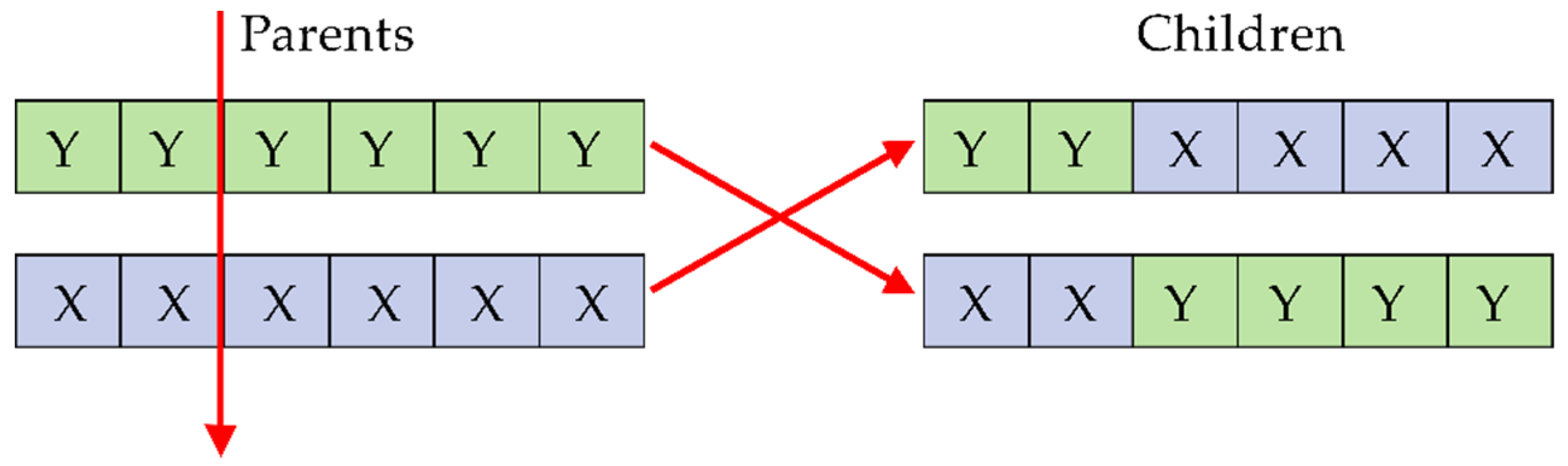
• Applying genetic operators on selected people in proliferation: By applying genetic operators on people, the children population is produced. Some of these operators are mentioned here:

  (A)

  Displacement: The approach of performing displacement on two strings that have been selected from a pond coupling is shown in Figure 1. The result of this action is producing two children.

  (B)

  Mutations: Random variation of a gene in each category is called mutation.

  (C)

  The translation operator: At this stage, a part of the string is selected and after translation placed in its position.

  (D)

  Selection: At the last stage, after generating children from the set of the initial population, children must be chosen for the next generation. For selection by the roulette wheel, race or elitism methods can be used.

By applying proliferation, displacement, mutation, and selection on a new generation again, the third generation can be produced. This generation will continue to make a stop condition [51].

Genetic algorithm has been used as a widely used optimization technique in various studies such as UC [52], wind energy studies [53], and path planning for self-reconfigurable robots [54].

3. Simulation and Discussion

This section focuses on different parts including the simulation parts, results, and discussions. It provides a concise and precise description of the experimental results, the interpretation, as well as the experimental conclusions that can be drawn.

3.1. Case Study

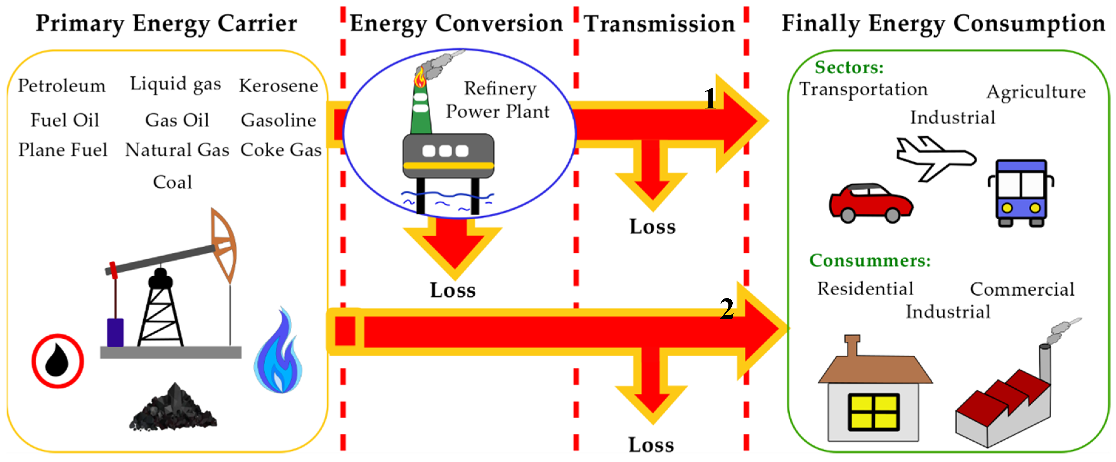
To illustrate the energy planning of primary energy carriers, a multi-carrier energy system with four power plants is used. The selected network contains transportation, industrial, and agriculture sectors; residential, commercial, and industrial consumers. Such parties are selected in the studied multi-carrier system for investigating a realistic viewpoint of interconnection among different energy carriers. The diagram of this studied multi-carrier system as well as its energy flow is drawn in Figure 2. In other words, Figure 2 shows the flow of energy from primary energy carriers to energy demand. Part of the energy demand is met directly from the primary energy carriers, which is indicated by arrow 2. Part of the energy demand is related to secondary energy carriers that become available after the energy conversion process in refineries or power plants. This concept is indicated by arrow 1. For example, electrical energy is a secondary energy carrier that is generated based on the conversion process of energy carriers in power plants. Information on this system is shown in

Table 1. Units data.

Power Plant	The Capacity of the Unit (MW)		Efficiency	Constant Cost ($)	Priority
	Min	Max
Thermal unit 1	75	400	0.368	700	1
Thermal unit 2	60	300	0.368	600	2
Combined Cycle unit	25	80	0.455	500	3
Gas unit	20	60	0.278	400	4

,

Table 2. Export and import of energy carriers.

Energy Carrier	Exported Energy (BOE)	Imported Energy (BOE)
Petroleum	63,576	0
Liquid gas	0	390.097
Fuel oil	3470.37	0
Gas oil	849.214	0
Kerosene	47.8092	0
Gasoline	0	3244.317
Plane fuel	0	467.2201
Natural gas	0	442.3143
Coke gas	5.76467	0
Coal	0	157.7139

,

Table 3. Initial conditions and timing data of units (hour).

Power Plant	Minimum Time of Running	Minimum Time of Shutting Down	Cold Start	Initial Conditions
Thermal unit 1	4	3	5	4
Thermal unit 2	4	2	4	4
Combined Cycle unit	3	1	3	4
Gas unit	2	1	2	−5

,

Table 4. Startup costs (US dollar).

Power Plant	Hot Start	Cold Start
Thermal unit 1	500	1100
Thermal unit 2	400	950
Combined Cycle unit	170	350
Gas unit	150	300

and

Table 5. Energy consumption for 24 h period Barrels of Oil Equivalent (BOE).

Hour	Residential, Commercial and Public	Industrial	Transportation	Agriculture	Other	Non-Energy
1	1300.973	633.221	801.9762	92.05099	6.734205	270.5027
2	1375.911	669.6951	848.1706	97.35321	7.122101	286.0839
3	1478.626	719.6897	911.489	104.6209	7.653786	307.4409
4	1617.767	787.4134	997.2612	114.4659	8.374016	336.3714
5	1647.586	801.9275	1015.643	116.5758	8.528372	342.5716
6	1748.432	851.0119	1077.809	123.7111	9.050377	363.5398
7	1792.539	872.4802	1104.999	126.832	9.278688	372.7107
8	1728.115	841.1231	1065.285	122.2736	8.945211	359.3154
9	1641.709	799.067	1012.021	116.1599	8.497951	341.3497
10	1702.912	828.8562	1049.749	120.4904	8.814754	354.0752
11	1440.681	701.2208	888.098	101.9361	7.457372	299.5512
12	1327.732	646.2451	818.4712	93.94429	6.872714	276.0664
13	1194.478	581.3864	736.3275	84.51583	6.182953	248.3597
14	1075.463	523.4585	662.9616	76.09488	5.566898	223.6138
15	970.6051	472.4213	598.3229	68.67563	5.024126	201.8114
16	835.9294	406.8708	515.3029	59.14658	4.327006	173.8092
17	845.3121	411.4376	521.0869	59.81046	4.375574	175.7601
18	855.4559	416.3749	527.3399	60.52819	4.428081	177.8692
19	867.4479	422.2118	534.7323	61.37669	4.490155	180.3627
20	1113.965	542.1985	686.6959	78.8191	5.766195	231.6192
21	1375.058	669.2801	847.6451	97.29288	7.117688	285.9066
22	1496.348	728.3153	922.4133	105.8748	7.745517	311.1256
23	1412.433	687.4714	870.6844	99.93734	7.311149	293.6776
24	1496.348	728.3153	922.4133	105.8748	7.745517	311.1256

. Some additional information is also provided in the Appendix A (

Table A1. Transmission matrix T_1,2.

Energy Carrier	Residential, Commercial and Public	Industrial	Transportation	Agriculture	Other	Non-Energy
Petroleum	0	0	0	0	0	0
Liquid gas	0.051	0.013	0.01	0	0	0
Fuel oil	0.023	0.212	0.014	0	0	0
Gas oil	0.055	0.087	0.363	0.689	0	0
Kerosene	0.141	0.002	0	0.018	0	0
Gasoline	0.002	0.002	0.573	0.003	0	0
Plane fuel	0	0	0.031	0	0	0
Other products	0	0	0	0	0	0.402
Natural gas	0.564	0.521	0.007	0	0	0.497
Coke gas	0	0.021	0	0	0	0
Coal	0.0003	0	0	0	0	0.101
Non-commercial fuels	0.064	0	0	0	0	0
Hydroelectric	0	0	0	0	0	0
Wind and solar	0	0	0	0	0	0
Electricity	0.102	0.142	0.0004	0.29	1	0
Nuclear	0	0	0	0	0	0

,

Table A2. T_p, P, and T_2,3.

Energy Carrier	Tp	T23	P
Petroleum	0	1	5858.1
Liquid gas	0.032	1	0
Fuel oil	0.293	1	0
Gas oil	0.293	1	0
Kerosene	0.099	1	0
Gasoline	0.157	1	0
Plane fuel	0	1	0
Other products	0.058	1	0
Natural gas	0	1.1601	3814.2
Coke gas	0	1	25.2
Coal	0	1	37.8
Non-commercial fuels	0	1	152.4
Hydroelectric	0	1	150.6
Wind and solar	0	1	0.6
Electricity (power)	0	1.3158	0
Nuclear	0	1	0

and

Table A3. Input rate of energy for power plant.

Unit	Steam	Steam	Combined Cycle	Gas
Fuel oil	0.254	0.254	0	0
Gas oil	0.003	0.003	0.082	0.166
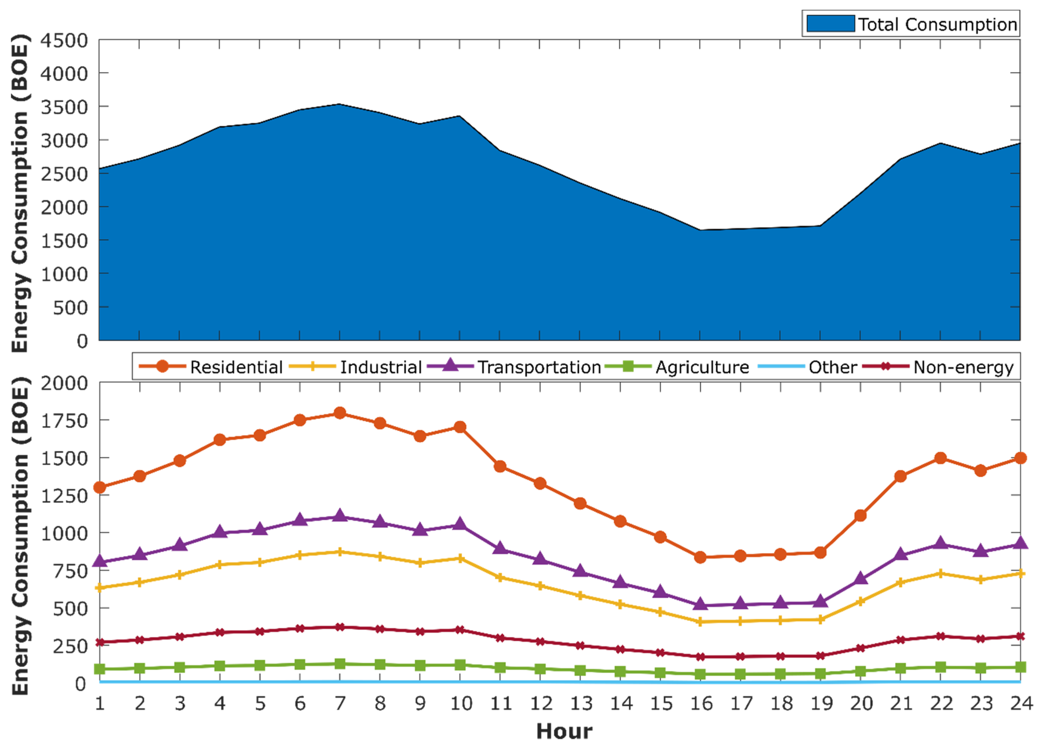
Natural gas	0.743	0.743	0.918	0.834

). The profile of energy demand is displayed in Figure 3. This figure shows the energy demand for all energy carriers (and not just electrical energy). Part of this energy demand is related to electricity demand, which is supplied by power plant units. Specifically, according to the information provided in Table 1 and Table 2, the peak demand for electricity in the seventh hour of the study is equal to 650.83122 MWh. This is while the maximum capacity of electricity production by the power plant units of this network is equal to 840 MWh. Therefore, the grid is able to supply the electricity demand.

3.2. ED and UC Solving

In recent years, various optimization algorithms have been introduced by researchers [55,56,57,58,59,60,61,62,63,64,65,66,67,68,69] and have been applied by scientists in various fields such as energy [70], protection [71], electrical engineering [72,73,74,75,76], energy carriers [77,78], and energy management [79,80] to achieve the optimal solution. Optimization algorithms have been always a popular way to solve ED and UC problems. In this paper, the economic distribution of electrical energy is done using GA. The objective functions of economic distribution of electrical energy are presented in Equations (10)–(13).

$$F_{obj}= {{\displaystyle \sum }}_{i=1}^{N_{FIU}}{E}_{FIU}^i C_{FIU}^i$$

(10)

$$E_{FIU}^i= {{\displaystyle \sum }}_{j=1}^{N_{DU}}{{\displaystyle \sum }}_{k=1}^{N_U^j}{e}_{i,j} E_{IU}^k \& i=1:N_{FIU}$$

(11)

$$e_{i,j}\in {\left[ETF\right]}_{N_{FIU}\times N_{DU}}$$

(12)

$$E_{IU}=\frac{1}{{ȵ}_U} E_{OU}$$

(13)

where $F_{obj}$ is the objective function, $N_{FIU}$ is the set of input fuels to power plants, $E_{FIU}^i$ is the whole energy input to power stations of fuel type i, $C_{FIU}^i$ is the fuel cost of plant type i, $N_{DU}$ is the set of different plants, $N_U^j$ is the set of plants of type j in the studied network, $e_{i,j}$ is the fuel contribution factor i from the plant’s energy input type j, $ETF$ is the input energy to fuel conversion matrix proportional to the plants, $E_{IU}$ is the input energy power plants matrix, ${ȵ}_U$ is the power plants efficiency vector, and $E_{OU}$ is the output electrical energy of power plants.

3.3. Determination of Optimization Constraints

The constraints include:

(1)

Power balance

$${{\displaystyle \sum }}_{i=1}^N{P}_i\left(t\right)=D\left(t\right)$$

(14)

(2)

Unit generation limits

$$P_{min}^i \le P^i\le P_{max}^i$$

(15)

where N is the number of plants, $P_i\left(t\right)$ is output power by the i^th unit at time t, $D\left(t\right)$ is the electric power demand at time t, $P_{min}^i$ is the minimum power, $P^i$ is output power, and $P_{max}^i$ indicates the maximum output power of the i^th plant.

3.4. Employement of Dynamic Programming

After the distribution of power at each time of planning, tailored to each energy division mode between power plants, the planning process continues and, therefore, an integration of energy carriers corresponding to the integration of plants is obtained. At this stage, energy strategy planning during the study period will be carried out using dynamic programming.

Recursive method for calculation of the least cost at hour K with the combination I, is as:

$$F_{cost}\left(K,I\right)= \underset{\left\{L\right\}}{\min }\left[P_{cost}\left(K,I\right)+S_{cost}\left(K-1,L:K,I\right)+F_{cost}\left(K-1,L\right)\right]$$

(16)

In Equation (16), $F_{cost}\left(K,I\right)$ is the minimum cost in order to achieve (K, I) state, $P_{cost}\left(K,I\right)$ is the cost of (K, I) state, and $S_{cost}\left(K-1, L:K,I\right)$ is the cost of transition from the state (K − 1, L) to (K, I). The (K, I) state is combination number I at hour K.

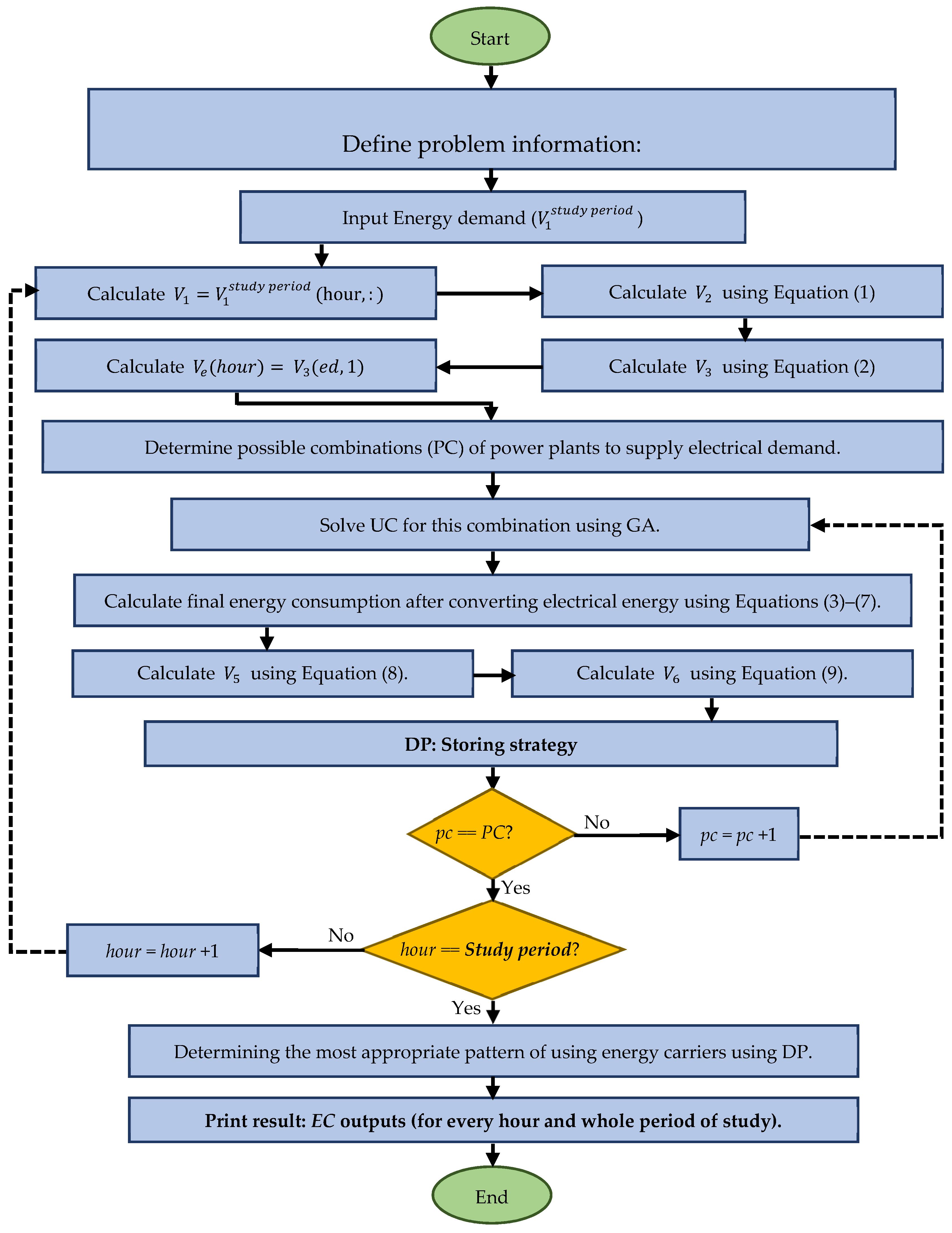
3.5. EC Implementation Steps

The various steps of EC are specified in Algorithm 1. The process of implementing the EC problem using flowchart is also shown in Figure 4.

Algorithm 1 Energy commitment (EC) implementation steps
START EC
1:	Problem information.
2:	Inputs data
3:	ITER = 1: Study period (24 h)
4:		$V_1=V_1^{study period }\left(ITER,:\right)$.
5:		$V_2$ calculation using Equation (1).
6:		$V_3$ calculation using Equation (2).
7:		$V_e=V_3\left(ed,1\right)$ and $ed$ = row number of electrical demand in $V_3$.
8:		UC solving
9:			Determine possible combinations of power plants to supply electrical demand.
10:			pc = 1
11:				While pc ≤ PC (PC = number of possible combinations).
12:					Economic dispatch (ED) solving for selected possible combination.
13:		End UC solving
14:					$V_4$ calculation using Equations (3)–(6).
15:					Refinery simulation using Equation (7).
16:					$V_5$ calculation using Equation (8).
17:					$V_6$ calculation using Equation (9).
18:					DP: Storing strategy
19:					pc = pc + 1
20:				END While
21:	END ITER
22:	EC outputs (for every hour and whole period of study)
23:		Determining the most appropriate pattern of using energy carriers
24:		Import and export of energy carriers
25:		Cost of energy supply
END EC

3.6. Experimental Setup

The proposed study is simulated on the mentioned energy network for a 24-h study period.

Genetic algorithm has been used as the optimization technique to solve the objective function. The number of chromosomes (population size) of the algorithm is equal to 50, the length of each chromosome is equal to 8, and the number of iterations is 50. The objective function has 8 variables. The 4 variables are related to the on or off status of power plant units and the other 4 variables are related to the amount of production of each of these units. In GA, the length of each chromosome is selected based on the number of problem variables. Therefore, the length of each chromosome is considered to be equal to 8.

4. Simulation Results

DP is done by storing the paths to the maximum number of hours of study modes. The correct strategy is the third case of combined units during the study period. The economic dispatch of electrical energy between the power plants units is specified in

Table 6. Economic distribution of power between the units.

Hour	Unit 1 Production (MW)	Unit 2 Production (MW)	Unit 3 Production (MW)	Unit 4 Production (MW)	Objective Function
1	170.6394	250	80	0	25,196.44
2	190.665	250	80	0	26,390.97
3	235.7225	250	80	0	29,078.68
4	250.7417	250	80	0	29,974.58
5	265.7609	250	80	0	30,870.48
6	290.7929	250	80	0	32,363.65
7	300	250	80	20.83122	34,155.45
8	285.8122	249.9998	79.99999	20	33,259.55
9	260.7801	250	80	20	31,766.38
10	240.7545	250	80	20.00002	30,571.85
11	210.7161	250	80	20	28,780.04
12	200.6778	250	80	0	26,988.24
13	120.5755	250	80	0	22,230.13
14	75	245.5115	79.99998	0	19,429.3
15	75	195.4476	80	0	16,630.42
16	75.00002	175.422	80	0	15,513.47
17	75	178.4259	79.99997	0	15,684.18
18	75.00003	183.4322	80	0	15,963.03
19	75	185.4348	80	0	16,067.62
20	75	205.4604	79.99998	0	17,188.08
21	80.52431	250	80	0	19,988.01
22	120.5755	250	80	0	22,228.1
23	170.6394	250	80	0	25,196.44
24	220.7033	250	80	0	28,182.78

. The need for energy carriers to provide final energy consumption over 24 h is given in

Table 7. Need for energy carriers in the energy network with 4 units using genetic algorithm (GA) (BOE).

Hour	Liquid Gas	Fuel Oil	Gas Oil	Kerosene	Gasoline	Plane Fuel	Natural Gas	Coke Gas	Coal
1	17.64232	−138.509	−26.9061	1.145155	143.2188	19.89864	1621.539	9.975951	22.04914
2	20.49007	−123.93	−9.56189	7.580451	159.7088	20.78303	1694.771	10.41933	23.02911
3	26.8975	−91.1249	29.46262	22.05987	196.8114	22.77289	1859.545	11.41692	25.23402
4	29.03331	−80.19	42.47079	26.88634	209.1789	23.43618	1914.469	11.74945	25.96899
5	31.16912	−69.2552	55.47896	31.71281	221.5464	24.09947	1969.394	12.08198	26.70396
6	34.7288	−51.0304	77.15924	39.75693	242.159	25.20495	2060.935	12.6362	27.92891
7	39.00043	−29.1606	103.1756	49.40987	266.894	26.53152	2170.784	13.30127	29.39886
8	36.86462	−40.0955	90.16741	44.5834	254.5265	25.86823	2115.859	12.96874	28.66389
9	33.30493	−58.3203	68.48713	36.53928	233.9139	24.76275	2024.318	12.41452	27.43893
10	30.45718	−72.9001	51.1429	30.10399	217.4239	23.87837	1951.086	11.97114	26.45897
11	26.18556	−94.7699	25.12656	20.45104	192.6889	22.55179	1841.237	11.30608	24.98903
12	21.91394	−116.64	−0.88977	10.7981	167.9538	21.22522	1731.388	10.64101	23.51909
13	10.52295	−174.814	−70.265	−14.9431	101.9937	17.68768	1438.882	8.867512	19.59924
14	3.403582	−209.916	−113.61	−31.0313	60.76859	15.47672	1259.74	7.759073	17.14933
15	−3.71579	−245.005	−156.954	−47.1196	19.54351	13.26576	1080.64	6.650634	14.69943
16	−6.56353	−259.022	−174.292	−53.5549	3.053474	12.38138	1009.055	6.207258	13.71947
17	−6.13637	−256.896	−171.691	−52.5896	5.526979	12.51403	1019.86	6.273765	13.86646
18	−5.42444	−253.395	−167.356	−50.9807	9.649487	12.73513	1037.748	6.384609	14.11145
19	−5.13966	−252.045	−165.623	−50.3372	11.29849	12.82357	1044.756	6.428946	14.20945
20	−2.29191	−238.003	−148.285	−43.9019	27.78852	13.70795	1116.415	6.872322	15.18941
21	4.827456	−202.906	−104.941	−27.8137	69.01361	15.91891	1295.538	7.980761	17.63931
22	10.52295	−174.828	−70.2651	−14.9431	101.9937	17.68768	1438.839	8.867512	19.59924
23	17.64232	−138.509	−26.9061	1.145155	143.2188	19.89864	1621.539	9.975951	22.04914
24	24.76169	−102.06	16.45445	17.23339	184.4438	22.1096	1804.62	11.08439	24.49905

. The need for energy carriers in the entire study period is given in

Table 8. Need for energy carriers in the entire study period in energy network.

Energy Carrier	Energy Demand (BOE)
Petroleum	34824
Liquid gas	390.097
Fuel oil	−3470.37
Gas oil	−849.214
Kerosene	−47.8092
Gasoline	3244.317
Plane fuel	467.2201
Natural gas	38122.31
Coke gas	234.2353
Coal	517.7139

. The export and import of energy carriers are shown in Table 2 with respect to the domestic production of energy carriers.

UC is one of the important outputs of EC study, which determines the on/off status and output of units for each hour of the study period. Table 6 presents the results of the UC. In this table, a power plant with zero production is off. The power plant with a production rate that has been determined is on. In the last column of this table, the value of the objective function for each hour of the study is presented. 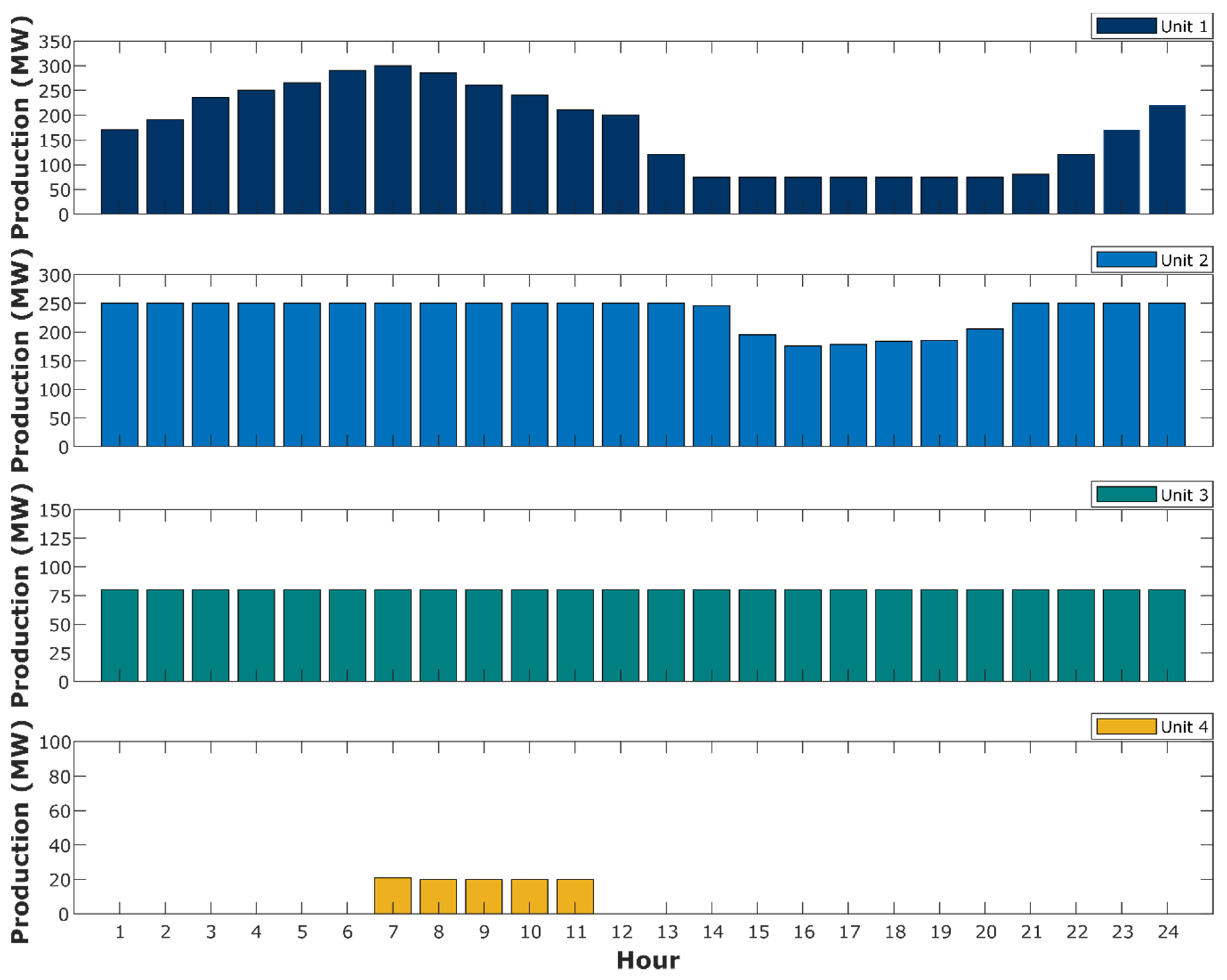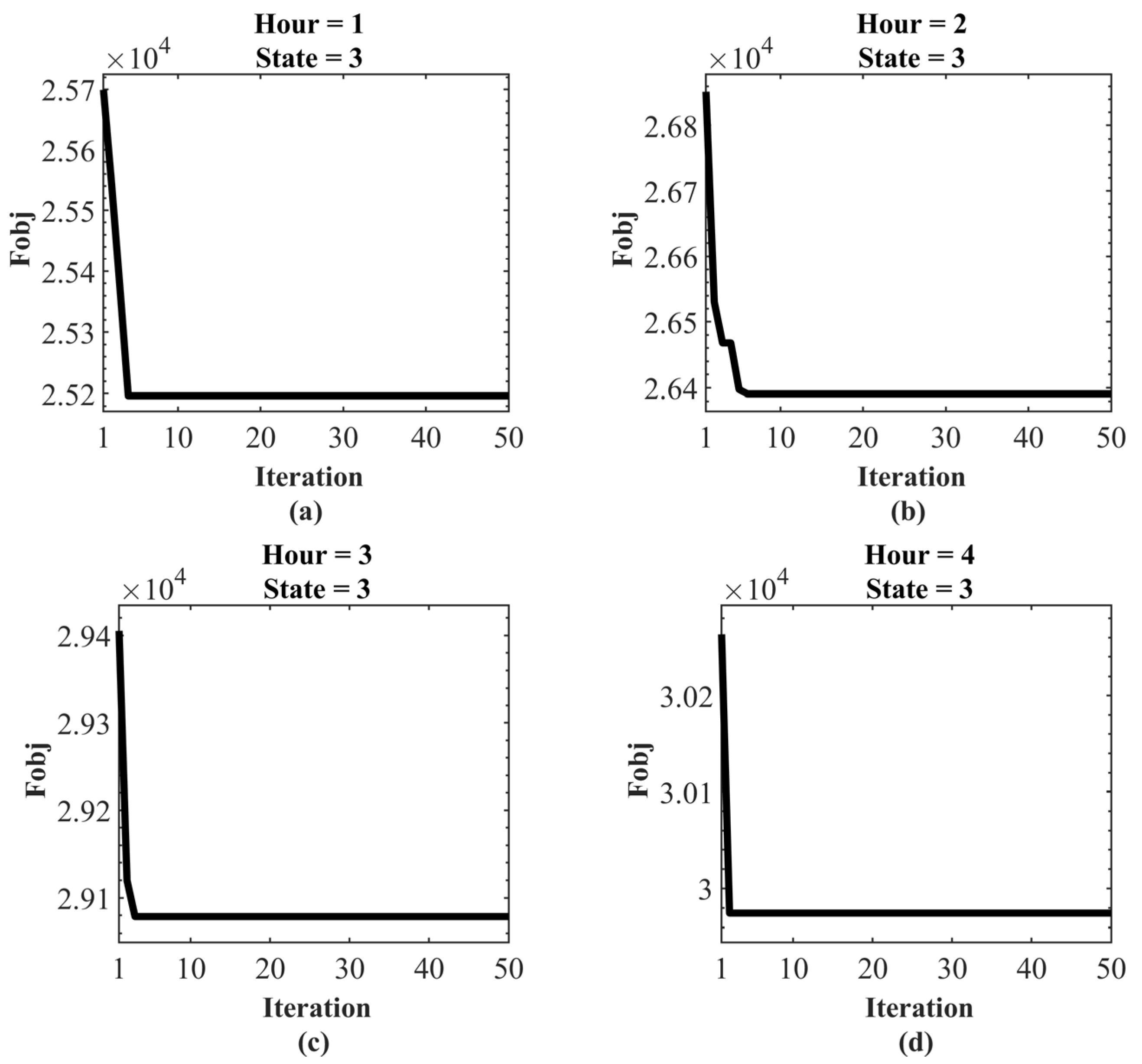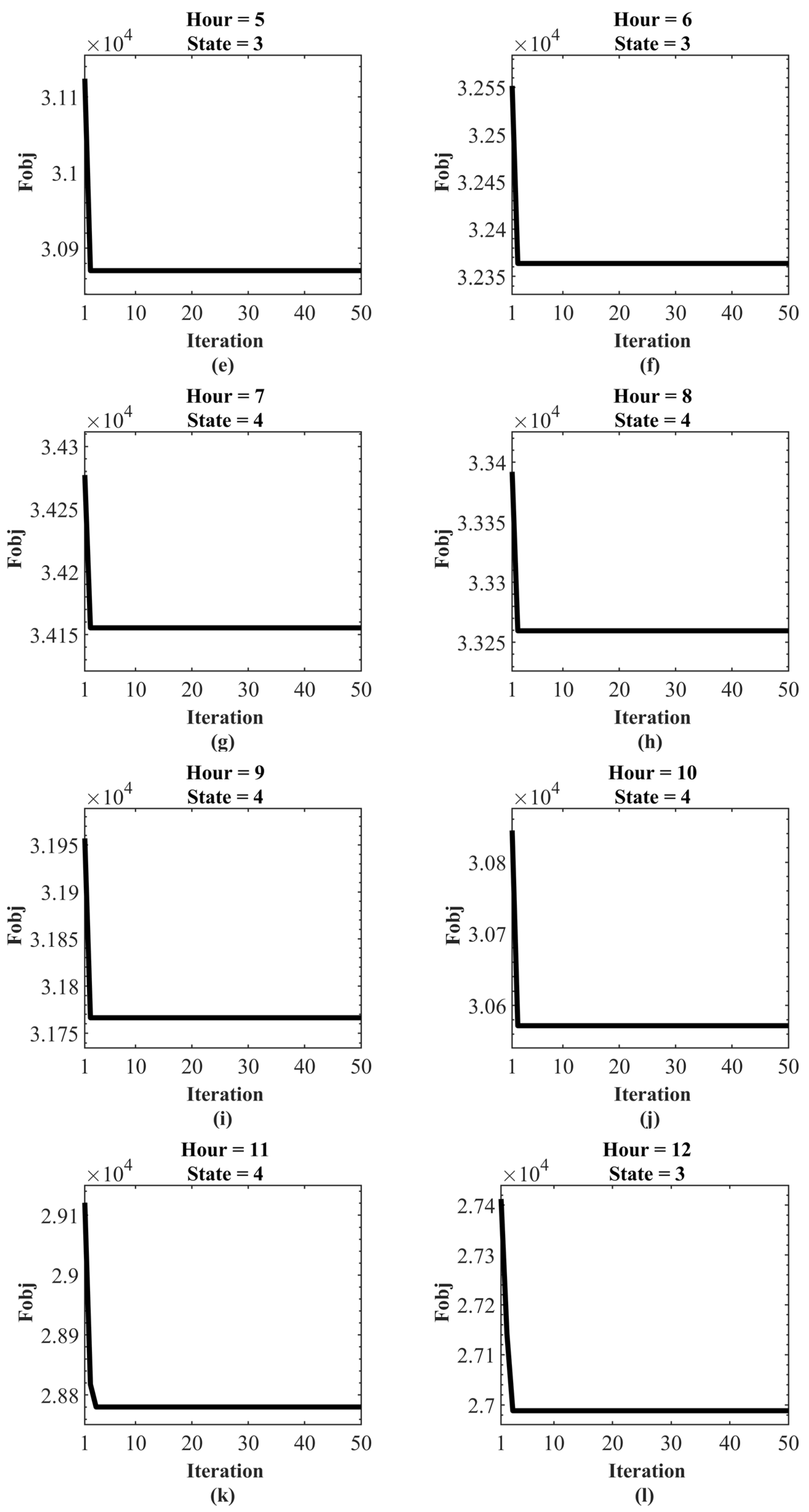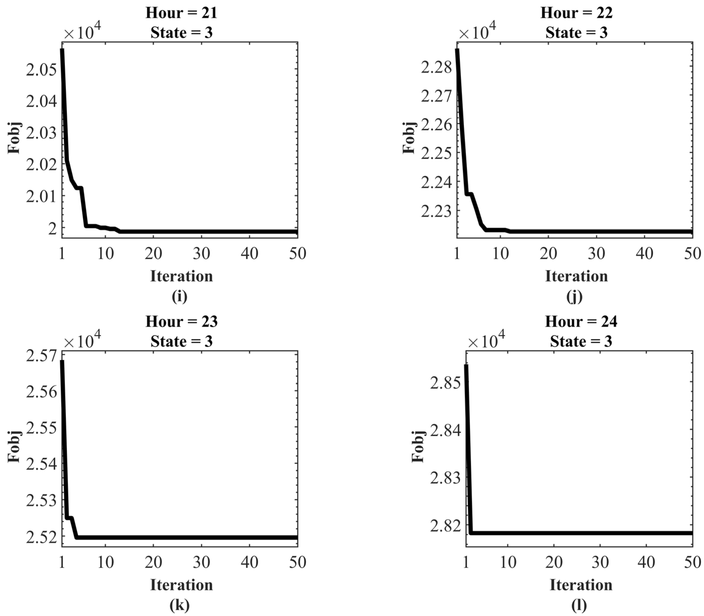Figure 5 shows the production profiles of the different units for the entire 24-h period. According to this figure, in the seventh hour of the study period, which is related to the highest peak of demand, the fourth unit turns on and then, with the decrease of demand, shut down in the 12th hour of the study period. The processes of achieving an optimal distribution of electrical energy between the units are shown in Figure 6andFigure 7. Figure 6 is for the first to twelfth hours of the study period and Figure 7 is for the thirteenth to twenty-fourth hours of the study period. In these figures, the convergence curves of the performance of the GA in the optimization of the objective function are shown as the best solution in terms of the iteration of the algorithm. The “state” in these figures shows the number of power plants on.

Another important outcome of the energy commitment study is to determine the appropriate pattern of use of energy carriers, which is presented in Table 7. In this table, the amount of need for nine energy carriers for each hour of the study period is specified separately. In this table, negative numbers indicate the excess of energy carrier production and positive numbers indicate the remaining need for energy carrier, which is supplied based on its domestic production.

Based on the amount of need for energy carriers per hour of the study period, the total amount of need for energy carriers for the entire study period can be calculated, which is presented in Table 8. In fact, Table 8 identifies the need for each energy carrier for the entire 24-h study period. The meaning of negative and positive numbers in this table is similar to Table 7.

The need for energy carriers is identified in Table 7 and Table 8, which must be supply using domestic products. But if domestic production is not enough to supply each of the energy carriers, that energy carrier must be supplied in the form of imports. Energy carriers that have surplus production also enter the export sector. Accordingly, the export and import volumes of different energy carriers as another output of the EC study are presented in Table 2.

5. Conclusions

Energy supply and demand in different types of energy carriers is one of the important challenges of the energy network. Operation of energy carriers in order to supply the energy demand of consumers at different energy levels requires accurate, technical, and economic planning. Therefore, in this paper, a new approach for energy studies is presented under the title of energy commitment (EC) in energy networks. In the proposed study, the energy network includes different parts of energy consumption that must be provided by appropriate energy carriers. The purpose of the EC study is to determine a technical and optimal pattern for the use of energy carriers in supply energy demand. The energy grid matrix model has been simulated step by step from the lowest energy level as the final energy consumption to the highest energy level, which is the primary energy carrier. Genetic algorithm (GA) has been used for the optimal allocation production share of each power plant unit in supplying electricity demand. At each hour of operation, different patterns of energy carriers are available to supply energy demand, and the best pattern must be selected. Dynamic planning (DP) method is used to determine the appropriate pattern of operation of energy carriers in the energy grid for the specified study period. The proposed EC study has been mathematically modeled and implemented on an energy grid with four power plants and different energy consumption sectors for a 24-h energy study period. In this simulation, an appropriate pattern of using energy carriers to supply energy demand has been determined. The presented results show clearly the proper strategy for economic scheduling of various units for energy production.

The authors express several items as suggestions and perspectives for future studies. Implementing the proposed study on different energy networks, using different optimization techniques to solve the EC problem, and considering different objective functions are study potentials for researchers. EC studies in the presence of newer generation sources such as photovoltaic and wind power plants also have a special potential for future studies.

References

1. Dong, Q.; Sun, Q.; Huang, Y.; Li, Z.; Cheng, C. Hybrid possibilistic-probabilistic energy flow assessment for multi-energy carrier systems. IEEE Access 2019, 7, 176115–176126. [Google Scholar] [CrossRef]
2. Nazari-Heris, M.; Mohammadi-Ivatloo, B.; Asadi, S. Optimal operation of multi-carrier energy networks with gas, power, heating, and water energy sources considering different energy storage technologies. J. Energy Storage 2020, 31, 101574. [Google Scholar] [CrossRef]
3. Yang, H.; Li, M.; Jiang, Z.; Zhang, P. Multi-time scale optimal scheduling of regional integrated energy systems considering integrated demand response. IEEE Access 2020, 8, 5080–5090. [Google Scholar] [CrossRef]
4. Shayan, H.; Amraee, T. Network constrained unit commitment under cyber attacks driven overloads. IEEE Trans. Smart Grid 2019, 10, 6449–6460. [Google Scholar] [CrossRef]
5. Morales-España, G.; Tejada-Arango, D.A. Modeling the hidden flexibility of clustered unit commitment. IEEE Trans. Power Syst. 2019, 34, 3294–3296. [Google Scholar] [CrossRef] [Green Version]
6. Safdarian, F.; Mohammadi, A.; Kargarian, A. Temporal decomposition for security-constrained unit commitment. IEEE Trans. Power Syst. 2019, 35, 1834–1845. [Google Scholar] [CrossRef]
7. Ning, C.; You, F. Data-driven adaptive robust unit commitment under wind power uncertainty: A Bayesian nonparametric approach. IEEE Trans. Power Syst. 2019, 34, 2409–2418. [Google Scholar] [CrossRef]
8. Li, X.; Zhai, Q.; Zhou, J.; Guan, X. A Variable reduction method for large-scale unit commitment. IEEE Trans. Power Syst. 2019, 35, 261–272. [Google Scholar] [CrossRef]
9. Geidl, M.; Andersson, G. Optimal power flow of multiple energy carriers. IEEE Trans. Power Syst. 2007, 22, 145–155. [Google Scholar] [CrossRef]
10. Moazeni, S.; Miragha, A.H.; Defourny, B. A risk-averse stochastic dynamic programming approach to energy hub optimal dispatch. IEEE Trans. Power Syst. 2018, 34, 2169–2178. [Google Scholar] [CrossRef]
11. Liu, T.; Zhang, D.; Dai, H.; Wu, T. Intelligent modeling and optimization for smart energy hub. IEEE Trans. Ind. Electron. 2019, 66, 9898–9908. [Google Scholar] [CrossRef]
12. Dolatabadi, A.; Jadidbonab, M.; Mohammadi-ivatloo, B. Short-term scheduling strategy for wind-based energy hub: A hybrid stochastic/IGDT approach. IEEE Trans. Sustain. Energy 2018, 10, 438–448. [Google Scholar] [CrossRef]
13. Shabanpour-Haghighi, A.; Seifi, A.R. Energy flow optimization in multicarrier systems. IEEE Trans. Ind. Inform. 2015, 11, 1067–1077. [Google Scholar] [CrossRef]
14. Nazari-Heris, M.; Mohammadi-Ivatloo, B.; Asadi, S. Optimal operation of multi-carrier energy networks considering uncertain parameters and thermal energy storage. Sustainability 2020, 12, 5158. [Google Scholar] [CrossRef]
15. Wang, H.; Gu, C.; Zhang, X.; Li, F. Optimal CHP planning in integrated energy systems considering network charges. IEEE Syst. J. 2019, 14, 2684–2693. [Google Scholar] [CrossRef] [Green Version]
16. Yan, M.; Zhang, N.; Ai, X.; Shahidehpour, M.; Kang, C.; Wen, J. Robust two-stage regional-district scheduling of multi-carrier energy systems with a large penetration of wind power. IEEE Trans. Sustain. Energy 2018, 10, 1227–1239. [Google Scholar] [CrossRef]
17. Kampouropoulos, K.; Andrade, F.; Sala, E.; Espinosa, A.G.; Romeral, L. Multiobjective optimization of multi-carrier energy system using a combination of ANFIS and genetic algorithms. IEEE Trans. Smart Grid 2016, 9, 2276–2283. [Google Scholar] [CrossRef] [Green Version]
18. Dictionary, E. World Energy Council; Jouve SI: Paris, France, 1992. [Google Scholar]
19. Kleinpeter, M. Fuel and energy abstracts. In Energy Planning and Policy; Elsevier: Amsterdam, The Netherlands, 1995; p. 382. [Google Scholar]
20. Bessanova, T.; Kulenov, N. Colloquium alma ata. In Econometric Models for Energy Consumption; United Nations: New York, NY, USA, 1973. [Google Scholar]
21. Prina, M.G.; Lionetti, M.; Manzolini, G.; Sparber, W.; Moser, D. Transition pathways optimization methodology through EnergyPLAN software for long-term energy planning. Appl. Energy 2019, 235, 356–368. [Google Scholar] [CrossRef]
22. Hemanth, J.; Balas, V.E. Nature Inspired Optimization Techniques for Image Processing Applications; Springer: New York, NY, USA, 2019. [Google Scholar]
23. Munier, N.; Hontoria, E.; Jiménez-Sáez, F. Linear programming fundamentals. In Strategic Approach in Multi-Criteria Decision Making; Springer: New York, NY, USA, 2019; pp. 101–116. [Google Scholar]
24. Hakki, A.; Schoor, A. Generation Planning System: Methodology and Case Study. Final Report. [LOADST]; Gordian Associates, Inc.: Hackensack, NJ, USA, 1981. [Google Scholar]
25. Wang, Y.; Wang, Y.; Huang, Y.; Li, F.; Zeng, M.; Li, J.; Wang, X.; Zhang, F. Planning and operation method of the regional integrated energy system considering economy and environment. Energy 2019, 171, 731–750. [Google Scholar] [CrossRef]
26. Cormio, C.; Dicorato, M.; Minoia, A.; Trovato, M. A regional energy planning methodology including renewable energy sources and environmental constraints. Ren. Sustain. Energy Rev. 2003, 7, 99–130. [Google Scholar] [CrossRef]
27. Hoog, D.T.; Hobbs, B.F. An integrated resource planning model considering customer value, emissions, and regional economic impacts. Energy 1993, 18, 1153–1160. [Google Scholar] [CrossRef]
28. Carvallo, J.P.; Larsen, P.H.; Sanstad, A.H.; Goldman, C.A. Long term load forecasting accuracy in electric utility integrated resource planning. Energy Policy 2018, 119, 410–422. [Google Scholar] [CrossRef] [Green Version]
29. Bhat, K.S.; Feichtinger, G.; Bachhiesl, U.; Stigler, H. Neu energie fur unser bewegtes europa. Model Based Analysis of the Indian Electricity Economics. In Proceedings of the 15th Symposium Energieinnovation: Neue Energie für Unser Bewegtes Europa, Graz University of Technology, Graz, Austria, 14–16 February 2018. [Google Scholar]
30. Monyei, C.; Adewumi, A. Integration of demand side and supply side energy management resources for optimal scheduling of demand response loads–South Africa in focus. Elec. Power Syst. Res. 2018, 158, 92–104. [Google Scholar] [CrossRef]
31. Krishnan, V.; Ho, J.; Hobbs, B.F.; Liu, A.L.; McCalley, J.D.; Shahidehpour, M.; Zheng, Q.P. Co-optimization of electricity transmission and generation resources for planning and policy analysis: Review of concepts and modeling approaches. Energy Syst. 2016, 7, 297–332. [Google Scholar] [CrossRef]
32. Hobbs, B.F.; Centolella, P. Environmental policies and their effects on utility planning and operations. Energy 1995, 20, 255–271. [Google Scholar] [CrossRef]
33. Hirst, E.; Goldman, C. Creating the future: Integrated resource planning for electric utilities. Ann. Rev. Energy Environ. 1991, 16, 91–121. [Google Scholar] [CrossRef]
34. Wang, C.-H.; Min, K.J. An integrated resource planning model for utilities with quantified outage costs. Int. J. Elect. Power Energy Syst. 1998, 20, 517–524. [Google Scholar] [CrossRef]
35. Busch, J.F.; Eto, J. Estimation of avoided costs for electric utility demand-side planning. Energy Sources 1996, 18, 473–499. [Google Scholar] [CrossRef]
36. Malik, A. Modelling and economic analysis of DSM programs in generation planning. Int. J. Elect. Power Energy Syst. 2001, 23, 413–419. [Google Scholar] [CrossRef]
37. Atikol, U. A demand-side planning approach for the commercial sector of developing countries. Energy 2004, 29, 257–266. [Google Scholar] [CrossRef]
38. Yang, M. Demand side management in Nepal. Energy 2006, 31, 2677–2698. [Google Scholar] [CrossRef]
39. World Bank Group. Sri Lanka—Energy Services Delivery Project; World Development Sources; World Bank: Washington, DC, USA, 1997. (In English) [Google Scholar]
40. World Bank Group. Sustainable Transport Options for Sri Lanka (Vol. 2): Greenhouse Gas Mitigation Options in the Sri Lanka Power Sector; World Bank Group: Washington, DC, USA, 2003. (In English) [Google Scholar]
41. Sotelo, D.; Favela-Contreras, A.; Sotelo, C.; Jiménez, G.; Gallegos-Canales, L. Design and implementation of a control structure for quality products in a crude oil atmospheric distillation column. ISA Trans. 2017, 71, 573–584. [Google Scholar] [CrossRef] [PubMed]
42. Sotelo, D.; Favela-Contreras, A.; Lozoya, C.; Beltran-Carbajal, F.; Dieck-Assad, G.; Sotelo, C. Dynamic simulation of a crude oil distillation plant using Aspen-Hysys®. Int. J. Simul. Model. 2019, 18, 229–241. [Google Scholar] [CrossRef]
43. Sotelo, C.; Favela-Contreras, A.; Sotelo, D.; Beltrán-Carbajal, F.; Cruz, E. Control structure design for crude oil quality improvement in a dehydration and desalting process. Arab. J. Sci. Eng. 2018, 43, 6579–6594. [Google Scholar] [CrossRef]
44. Barbir, F. Transition to renewable energy systems with hydrogen as an energy carrier. Energy 2009, 34, 308–312. [Google Scholar] [CrossRef]
45. Krause, T.; Andersson, G.; Frohlich, K.; Vaccaro, A. Multiple-energy carriers: Modeling of production, delivery, and consumption. Proc. IEEE 2011, 99, 15–27. [Google Scholar] [CrossRef]
46. Ridjan, I.; Mathiesen, B.V.; Connolly, D.; Duić, N. The feasibility of synthetic fuels in renewable energy systems. Energy 2013, 57, 76–84. [Google Scholar] [CrossRef] [Green Version]
47. Amoo, L.M.; Fagbenle, R.L. An integrated impact assessment of hydrogen as a future energy carrier in Nigeria’s transportation, energy and power sectors. Int. J. Hydrogen Energy 2014, 39, 12409–12433. [Google Scholar] [CrossRef]
48. Trop, P.; Goricanec, D. Comparisons between energy carriers’ productions for exploiting renewable energy sources. Energy 2015, 108, 155–161. [Google Scholar] [CrossRef]
49. Geng, W.; Ming, Z.; Lilin, P.; Ximei, L.; Bo, L.; Jinhui, D. China׳ s new energy development: Status, constraints and reforms. Ren. Sustain. Energy Rev. 2016, 53, 885–896. [Google Scholar] [CrossRef]
50. Beller, M.; Cherniavsky, E.; Hoffman, K.; Williamson, R. Interfuel Substitution Study: The Role of Electrification; Brookhaven National Lab., Upton: New York, NY, USA, 1974. [Google Scholar]
51. Mirjalili, S. Genetic algorithm. In Evolutionary Algorithms and Neural Networks; Springer: New York, NY, USA, 2019; pp. 43–55. [Google Scholar]
52. Jo, K.-H.; Kim, M.-K. Improved genetic algorithm-based unit commitment considering uncertainty integration method. Energies 2018, 11, 1387. [Google Scholar] [CrossRef] [Green Version]
53. Teh, J.; Lai, C.-M.; Cheng, Y.-H. Improving the penetration of wind power with dynamic thermal rating system, static VAR compensator and multi-objective genetic algorithm. Energies 2018, 11, 815. [Google Scholar] [CrossRef] [Green Version]
54. Le, A.V.; Arunmozhi, M.; Veerajagadheswar, P.; Ku, P.-C.; Minh, T.Q.; Sivanantham, V.; Mohan, R.E. Complete path planning for a tetris-inspired self-reconfigurable robot by the genetic algorithm of the traveling salesman problem. Electronics 2018, 7, 344. [Google Scholar] [CrossRef] [Green Version]
55. Dehghani, M.; Montazeri, Z.; Dehghani, A.; Seifi, A. Spring search algorithm: A new meta-heuristic optimization algorithm inspired by Hooke’s law. In Proceedings of the IEEE 4th International Conference on Knowledge-Based Engineering and Innovation (KBEI), Tehran, Iran, 22 December 2017; pp. 210–214. [Google Scholar]
56. Dehghani, M.; Montazeri, Z.; Dehghani, A.; Nouri, N.; Seifi, A. BSSA: Binary spring search algorithm. In Proceedings of the IEEE 4th International Conference on Knowledge-Based Engineering and Innovation (KBEI), Tehran, Iran, 22 December 2017; pp. 220–224. [Google Scholar]
57. Dehghani, M.; Montazeri, Z.; Malik, O.P.; Ehsanifar, A.; Dehghani, A. OSA: Orientation search algorithm. Int. J. Ind. Electron. Control Optim. 2019, 2, 99–112. [Google Scholar]
58. Dehghani, M.; Montazeri, Z.; Malik, O.P.; Dhiman, G.; Kumar, V. BOSA: Binary orientation search algorithm. Int. J. Innov. Technol. Explor. Eng. IJITEE 2019, 9, 5306–5310. [Google Scholar]
59. Dehghani, M.; Montazeri, Z.; Malik, O.P. DGO: Dice game optimizer. Gazi Univ. J. Sci. 2019, 32, 871–882. [Google Scholar] [CrossRef] [Green Version]
60. Dehghani, M.; Montazeri, Z.; Dehghani, A.; Malik, O.P. GO: Group Optimization. Gazi Univ. J. Sci. 2020, 33, 381–392. [Google Scholar] [CrossRef]
61. Mohammad, D.; Zeinab, M.; Malik, O.P.; Givi, H.; Guerrero, J.M. Shell game optimization: A novel game-based algorithm. Int. J. Intel. Eng. Syst. 2020, 13, 10. [Google Scholar]
62. Dehghani, M.; Montazeri, Z.; Saremi, S.; Dehghani, A.; Malik, O.P.; Al-Haddad, K.; Guerrero, J.M. HOGO: Hide Objects Game Optimization. Int. J. Intell. Eng. Syst. 2020, 13, 10. [Google Scholar] [CrossRef]
63. Dehghani, M.; Mardaneh, M.; Malik, O.P.; NouraeiPour, S.M. DTO: Donkey theorem optimization. In Proceedings of the 27th Iranian Conference on Electrical Engineering (ICEE), Tehran, Iran, 30 April–2 May 2019; pp. 1855–1859. [Google Scholar]
64. Gaurav, D.; Meenakshi, G.; Atulya, K.N.; Vijay, K.; Dehghani, M. A novel algorithm for global optimization: Rat swarm optimizer. J. Amb. Intel. Hum. Comput. 2020. [Google Scholar] [CrossRef]
65. Dehghani, M.; Mardaneh, M.; Malik, O. FOA: Following Optimization Algorithm for solving power engineering optimization problems. J. Oper. Automat. Power Eng. 2020, 8, 57–64. [Google Scholar]
66. Dehghani, M.; Montazeri, Z.; Givi, H.; Guerrero, J.M.; Dhiman, G. Darts game optimizer: A new optimization technique based on darts game. Int. J. Intell. Eng. Syst. 2020, 13. [Google Scholar] [CrossRef]
67. Dehghani, M.; Samet, H. Momentum search algorithm: A new meta-heuristic optimization algorithm inspired by momentum conservation law. SN Appl. Sci. 2020, 2, 1–15. [Google Scholar] [CrossRef]
68. Dehghani, M.; Montazeri, Z.; Dehghani, A.; Samet, H.; Sotelo, C.; Sotelo, D.; Ehsanifar, A.; Malik, O.P.; Guerrero, J.M.; Dhiman, G. DM: Dehghani Method for modifying optimization algorithms. Appl. Sci. 2020, 10, 7683. [Google Scholar] [CrossRef]
69. Dehghani, M.; Montazeri, Z.; Dehghani, A.; Ramirez-Mendoza, R.A.; Samet, H.; Guerrero, J.M.; Dhiman, G. MLO: Multi leader optimizer. Int. J. Intell. Eng. Syst. 2020, 13, 364–373. [Google Scholar] [CrossRef]
70. Dehghani, M.; Montazeri, Z.; Malik, O. Energy commitment: A planning of energy carrier based on energy consumption. Electr. Eng. Electromec. 2019. [Google Scholar] [CrossRef]
71. Ehsanifar, A.; Dehghani, M.; Allahbakhshi, M. Calculating the leakage inductance for transformer inter-turn fault detection using finite element method. In Proceedings of the Iranian Conference on Electrical Engineering (ICEE), Tehran, Iran, 2–4 May 2017; pp. 1372–1377. [Google Scholar]
72. Dehghani, M.; Montazeri, Z.; Malik, O. Optimal sizing and placement of capacitor banks and distributed generation in distribution systems using spring search algorithm. Int. J. Emerg. Electric Power Syst. 2020, 21. [Google Scholar] [CrossRef] [Green Version]
73. Dehghani, M.; Montazeri, Z.; Malik, O.P.; Al-Haddad, K.; Guerrero Josep, M.; Dhiman Gaurav, A. New methodology called dice game optimizer for capacitor placement in distribution systems. Electr. Eng. Electromec. 2020. [Google Scholar] [CrossRef] [Green Version]
74. Dehbozorgi, S.; Ehsanifar, A.; Montazeri, Z.; Dehghani, M.; Seifi, A. Line loss reduction and voltage profile improvement in radial distribution networks using battery energy storage system. In Proceedings of the IEEE 4th International Conference on Knowledge-Based Engineering and Innovation (KBEI), Tehran, Iran, 22 December 2017; pp. 215–219. [Google Scholar]
75. Montazeri, Z.; Niknam, T. Optimal utilization of electrical energy from power plants based on final energy consumption using gravitational search algorithm. Electr. Eng. Electromec. 2018. [Google Scholar] [CrossRef] [Green Version]
76. Dehghani, M.; Mardaneh, M.; Montazeri, Z.; Ehsanifar, A.; Ebadi, M.; Grechko, O. Spring search algorithm for simultaneous placement of distributed generation and capacitors. Electr. Eng. Electromec. 2018. [Google Scholar] [CrossRef]
77. Dehghani, M.; Montazeri, Z.; Ehsanifar, A.; Seifi, A.; Ebadi, M.; Grechko, O. Planning of energy carriers based on final energy consumption using dynamic programming and particle swarm optimization. Electr. Eng. Electromec. 2018. [Google Scholar] [CrossRef] [Green Version]
78. Montazeri, Z.; Niknam, T. Energy carriers management based on energy consumption. In Proceedings of the 4th International Conference on Knowledge-Based Engineering and Innovation (KBEI), Tehran, Iran, 22 December 2017; pp. 0539–0543. [Google Scholar]
79. Huang, Y.; Yang, K.; Zhang, W.; Lee, K.Y. Hierarchical Energy Management for the multienergy carriers system with different interest bodies. Energies 2018, 11, 2834. [Google Scholar] [CrossRef] [Green Version]
80. Li, J.; Niu, D.; Wu, M.; Wang, Y.; Li, F.; Dong, H. Research on battery energy storage as backup power in the operation optimization of a regional integrated energy system. Energies 2018, 11, 2990. [Google Scholar] [CrossRef] [Green Version]
Figure 1. Displacement action.
Sustainability 12 10053 g001
Figure 2. Energy network flow.
Sustainability 12 10053 g002
Figure 3. Energy demand profile.
Sustainability 12 10053 g003
Figure 4. Flowchart of energy commitment (EC) problem.
Sustainability 12 10053 g004
Figure 5. The units productions on study period.
Sustainability 12 10053 g005
Figure 6. The process of achieving optimal distribution of electrical energy. (al) means hours 1 to 12.
Sustainability 12 10053 g006aSustainability 12 10053 g006b
Figure 7. The process of achieving optimal distribution of electrical energy. (al) means hours 13 to 24.
Sustainability 12 10053 g007aSustainability 12 10053 g007b