
HF-SPHR: Hybrid Features for Sustainable Physical Healthcare Pattern Recognition Using Deep Belief Networks


1
Department of Computer Science, Air University, Islamabad 44000, Pakistan
2
Department of Computer Science and Software Engineering, United Arab Emirates University, Al Ain 15551, United Arab Emirates
3
Department of Human-Computer Interaction, Hanyang University, Ansan 15588, Korea
*
Author to whom correspondence should be addressed.
Sustainability 2021, 13(4), 1699; https://0-doi-org.brum.beds.ac.uk/10.3390/su13041699
Submission received: 18 December 2020
/
Revised: 29 January 2021
/
Accepted: 31 January 2021
/
Published: 4 February 2021
(This article belongs to the Special Issue Sustainable Human-Computer Interaction and Engineering)
Abstract
:The daily life-log routines of elderly individuals are susceptible to numerous complications in their physical healthcare patterns. Some of these complications can cause injuries, followed by extensive and expensive recovery stages. It is important to identify physical healthcare patterns that can describe and convey the exact state of an individual’s physical health while they perform their daily life activities. In this paper, we propose a novel Sustainable Physical Healthcare Pattern Recognition (SPHR) approach using a hybrid features model that is capable of distinguishing multiple physical activities based on a multiple wearable sensors system. Initially, we acquired raw data from well-known datasets, i.e., mobile health and human gait databases comprised of multiple human activities. The proposed strategy includes data pre-processing, hybrid feature detection, and feature-to-feature fusion and reduction, followed by codebook generation and classification, which can recognize sustainable physical healthcare patterns. Feature-to-feature fusion unites the cues from all of the sensors, and Gaussian mixture models are used for the codebook generation. For the classification, we recommend deep belief networks with restricted Boltzmann machines for five hidden layers. Finally, the results are compared with state-of-the-art techniques in order to demonstrate significant improvements in accuracy for physical healthcare pattern recognition. The experiments show that the proposed architecture attained improved accuracy rates for both datasets, and that it represents a significant sustainable physical healthcare pattern recognition (SPHR) approach. The anticipated system has potential for use in human–machine interaction domains such as continuous movement recognition, pattern-based surveillance, mobility assistance, and robot control systems.
1. Introduction
The global elderly population is increasing every day, which requires an independent and aging-in-place lifestyle [1]. Research on Sustainable Physical Healthcare Pattern Recognition (SPHR) has a long tradition, because physical activity recognition can deliver great benefits to society. However, complex SPHR remains a challenging and active research area. A commonly-used strategy is to acquire, analyze, and classify the data for physical activity recognition [2]. It has a wide range of applications, including video surveillance systems, healthcare monitoring, uncertain event detection, interactive 3D games, and smart homes [3]. In order to examine the effectiveness of SPHR for indoor/outdoor environments, the major systems are categorized into two types of data retrieval devices, namely, vision-based and wearable-sensors–based [4]. In vision-based systems, SPHR is relatively prominent, and has been studied extensively, providing acceptable recognition rates. It is challenging to accomplish vision-based setups in real-life environments due to elevated acquisition costs, privacy issues, and image collection challenges. Wearable systems can exploit common portable devices with embedded sensors due to their low cost, portability, convenience, and capacity to log the real-time physical locomotion of users. Therefore, due to such valuable features and affordances, our research work is focused on wearable hybrid features for sustainable physical healthcare Pattern Recognition (HF-SPHR) technology.
Meanwhile, several studies involving wearable devices have been proposed by researchers. These can be categorized by two main types of learning algorithm, namely, classical machine learning (C-ML) and deep learning (DL). In the case of C-ML, the algorithms almost always require structured data, and are designed to ‘learn’ to act by understanding labeled data. Every time the result is incorrect, there is a need to ‘teach’ them again. On the other hand, DL methods help in handling the imperfections of C-ML techniques, and do not require human interventions, as the multi-layers in artificial neural networks (ANN) store data in a hierarchy of different models. This hierarchy consists of three types of layers which support the networks to learn from their own mistakes, specifically, input, output, and hidden layers.
Specific to DL concepts, recent theoretical and practical developments have revealed that deep learning has embraced visible changes in the modeling of high-level perceptions from convoluted data in many research areas [5], e.g., computer vision, natural language processing, and speech processing. Various deep learning methods have become available for SPHR in recent research, including deep neural networks (DNN), recurrent neural networks (RNN), and modular neural networks (MNN). DNN include auto-encoders, convolution neural networks (CNN), restricted Boltzmann machines (RBM), and long short-term memory (LSTM) [6]. LSTM requires longer training periods due to a variety of parameters being updated during the training process [7]. Similarly, CNN is able to learn important features [8], but—due to its single-parameter setting—the limited flexibility of the model has been observed. Meanwhile, RBMs are fully-connected, bipartite, and undirected graphs that have both a visible and a hidden layer, and are examples of artificial neural networks [9]. If stacked together, they create a deep belief network (DBN) [10]. DBNs are probabilistic generative neural networks that use the connection weights of cross-layered RBM architecture. RBMs detect the features of data between different classes according to the connection weights across two layers, and not within each layer. When trained, a DBN can learn to reconstruct its input, and the layers act as feature detectors. After the unsupervised learning, a DBN can be further trained, with supervision, to perform classification. Therefore, our model encircles the properties of DBN and RBMs.
There are two well-known ways to investigate SPHR, namely, vision-based SPHR and wearable-sensors–based SPHR, which are applied in studies of both C-ML and DL. Vision-based SPHR is dependent on visual sensing technologies, namely, CCTV and digital cameras. Sequences of images and video clips are analyzed for features, modelling, segmentations, classification, and tracking [11]. Jalal et al. [12] proposed a depth vision-based model for activity recognition using hidden Markov models (HMM) to monitor the activities of elderly individuals. Multiple features are fused together to make robust multi-features, which are then processed, trained, and tested with respect to their classes. Espinosa et al. [13] designed a fall-detection system using 2D CNN and multiple cameras. They presented a method with fixed time windows and an optical flow method for feature extraction for an UP-Fall dataset in order to test the proposed approach. In [14], the authors proposed human pose estimation and event classification using a pseudo-2D stick model. They used energy, sine, distinct body parts movements, and 3D Cartesian view features to extract full-body human silhouettes. Yang and Tian [15] described a low-level polynormal assembled from a local neighboring hypersurface. A methodology including hybrid feature descriptors, GMM, entropy optimization, and maximum entropy Markov model (MEMM)-based classification was developed by Jalal et al. in [16]. Mahmood et al. [17] presented a model for human interaction recognition called WHITE STAG. Angular-geometric sequential methods based on space, time, and shape have been incorporated to extract features. In [18], Jalal et al. represented a technique using spatiotemporal multi-fused features to classify segmented human activity. The proposed study used vector quantization for code vector generation, and HMM for SPHR.
On the other hand, wearable sensors can be attached to the human body in order to capture human motion data constantly. In [19], Irvine et al. focused on data-driven approaches and proposed a new ensemble of neural networks. The authors generated four base models and integrated them using a support function fusion method to compute the output decision score for each base classifier. In a study of wearable sensors by Xi et al. [20], surface electromyography (sEMG) wearable sensors are attached on the limbs to monitor the performance of daily activities for frail individuals. They proposed time-, frequency- and entropy-based feature abstraction. Gaussian Kernel Support Vector Machines (GK-SVM) and Fuzzy Min-Max Neural Networks (FMMNN) are used for activity classification. In [21], Wijekoon et al. described a knowledge-light method, as opposed to knowledge intensive methods. They proposed the use of a few seconds of data to help personalize SPHR models, and to further transfer recognition knowledge to identify unknown activities. In [22], Quaid et al. introduced a human pattern behavior recognition method using inertial sensors. They proposed extracting statistical, cepstral, temporal, and spectral features, and then reweighting these features to adapt varying signal patterns. Finally, the classification is performed using biological operations of crossover and mutation. Tahir et al. [23] presented a wearable inertial sensor-based activity recognition system using filters and multifused features. Feature optimization has been accomplished using adaptive moment estimation (Adam) and AdaDelta, which is further patterned using MEMM. Debache et al. The authors of [24] proposed a low-complexity model that is comparable to heavily-featured models for SPHR. They used mobile health (mHealth) and daily Life Activity (DaLiAc) datasets to compare their model’s performance using logistic regression (LR), gradient boosting (GB), k-nearest-neighbors (KNN), support vector machines (SVM), and CNN. The authors of [25] proposed a novel method based on the Human Gait Database (HuGaDB) dataset. Their contributions include the identification of direction and sensor position, a best feature selection method, and achieving the highest recognition accuracy for HuGaDB. Furthermore, the model has four different classifiers, namely, Random Forest [26] (RF), SVM, KNN, and Decision Tree (DT). Jalal et al. [27] presented a genetic-based classifier approach for human activity recognition. They proposed a reweighted genetic algorithm for SPHR using inertial data.
Considering our focal schema, we know that SPHR is eventually associated to the real-time monitoring of activities. Additionally, it contains tradeoffs between computational time and activity pattern recognition accuracies. In spite of all of these advanced research methodologies being proposed, there is still a deficiency in the classification of human activities using state-of-the-art techniques. Thus, our research is dedicated to the development of an efficient method that maintains high accuracy rates along with low computational complexities.
Here, we propose an innovative methodology for SPHR using wearable sensors, including an inertial measurement unit (IMU), electrocardiography (ECG), and electromyography (EMG). Our model was able to recognize diverse human activities with better performance measures. Moreover, the proposed methodology consists of de-noising signals, pre-processing, and hybrid feature abstraction. For hybrid features, this research proposed the following four types of features:
- Statistical nonparametric operator; i.e., a 1D local binary pattern (1D-LBP) generates a code [28] that can describe larger data in its compressed form using the sample and its neighbors.
- Entropy-based features: these features are used to find the optimal characteristics of a signal [29], and can easily differentiate between noisy and plain signals.
After extracting the hybrid features, the proposed model performs feature-to-feature fusion, feature selection, a codebook using Gaussian models, and classification for state-of-the-art datasets. Through experimental results, we showed that the proposed model outperformed other comparative state-of-the-art approaches. The major contributions of this model are as follows:
- We developed hybrid approaches for feature abstraction, including statistical nonparametric, entropy-based, wavelet transform, and Mel-cepstral features.
- We designed a multi-layer sequential forward selection (MLSFS) to differentiate and select the optimal features for SPHR.
- A combination of a Gaussian mixture model (GMM) with Gaussian mixture regression (GMR) was introduced to generate the codebook and optimum interpretation of the features.
- We used two publicly-available benchmark datasets for our model, and fully validated it against other state-of-the-art methods, including CNN, AdaBoost, and ANN-based algorithms.
The rest of the paper is structured as follows. Section 2 presents the details of the proposed model. Section 3 reports on the investigation and dataset details, along with the results. Section 4 discusses the methodology. Section 5 reports related discussions in the field of SPHR. Section 5 concludes the paper and provides some forthcoming directions.
2. Materials and Methods
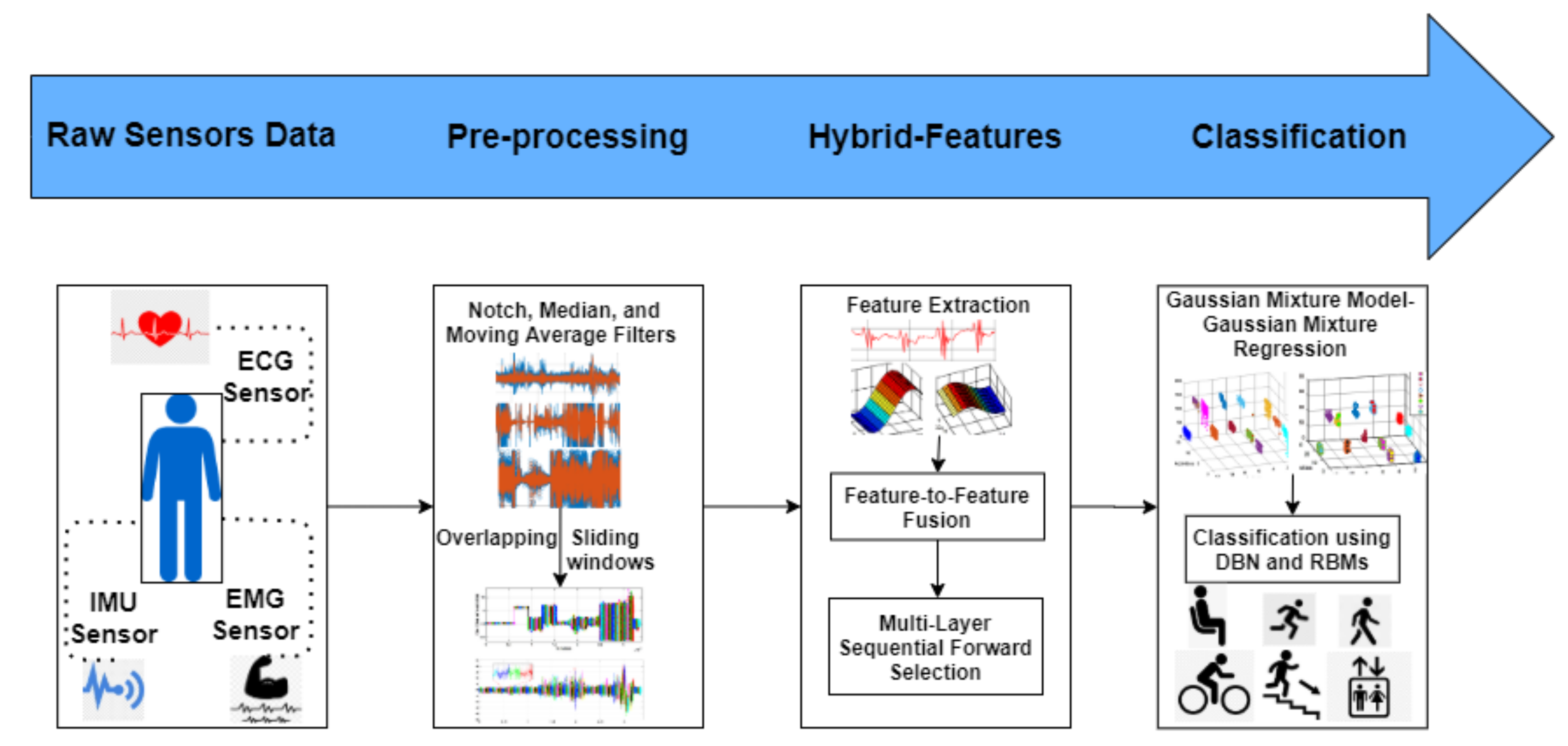
The proposed system acquires raw signals from wearable sensors, specifically, an inertial measurement unit, an electrocardiogram, and an electromyogram for biosignal-based datasets. Initially, a pre-processing phase is used to remove any noise via three different filters, namely, median, notch, and moving average filters. After that, we apply a sliding window algorithm to find hybrid features of different types [34]. In the perspective of multisensory systems, these hybrid features are then fused [35] through a feature-in-feature-out technique [36,37] to improve, refine, and obtain new merged features. The dimensions of these fused data features are reduced using our novel modified multi-layer sequential forward selection algorithm. Next, in order to symbolize these reduced features, we propose a GMM along with GMR algorithms to generate a codebook. Finally, the codebook is then fed to the deep belief networks along with multiple layers of RBMs. An overview of the proposed system is shown in the Figure 1.
2.1. Data Acquisition and Pre-Processing
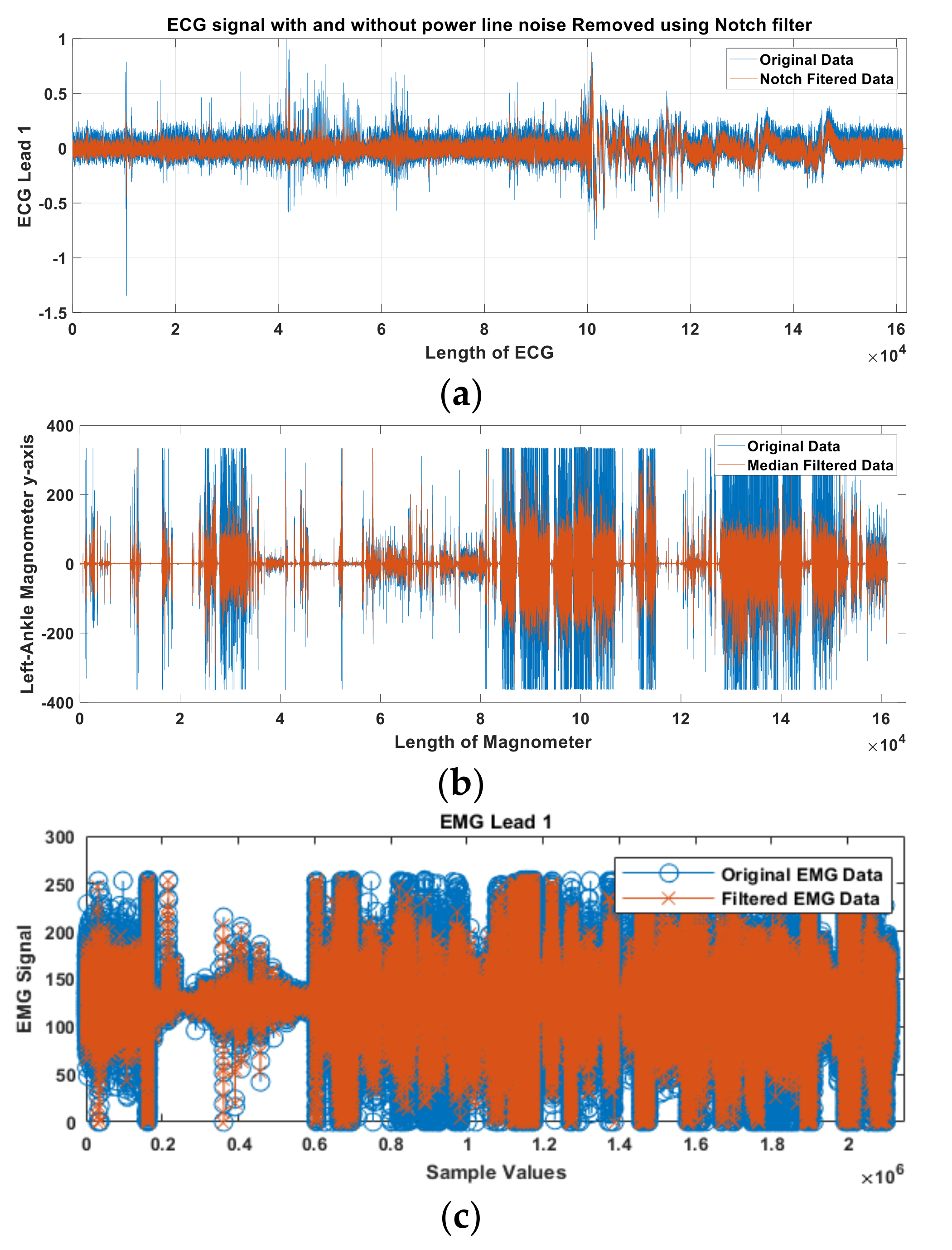
Feature abstraction is deeply reliant on the pre-processing phase; hence, it is important to reduce all of the noise from the acquired data. The data from the sensors [38]—including IMU, ECG, and EMG—are extremely susceptible to interference and random noise, which can lead to signal variations, ultimately affecting the features. Therefore, we have applied three different filter types—namely, a median filter for IMU, a notch filter for ECG, and a moving average filter for EMG signals—to eliminate the associated noise. Figure 2 shows the filtering effects on selected lead for ECG, and the axis for IMU.
2.2. Data Segmentation
In the segmentation step, the signal samples are partitioned into segments of data in order to capture the dynamic motion. Each window is an approximation of the signal, which is provided for the signal analytics. We can segment a signal in different ways, as activity-defined windows, event-defined windows and sliding windows [39,40]. After the filtering in the pre-processing step, we segmented the filtered data using widows of 5 s duration for each of the signals’ axes and ECG/EMG leads, as defined in Algorithm 1, in order to maximize the recognition accuracy.
| Algorithm 1 Signals Overlapping Segmentation |
 |
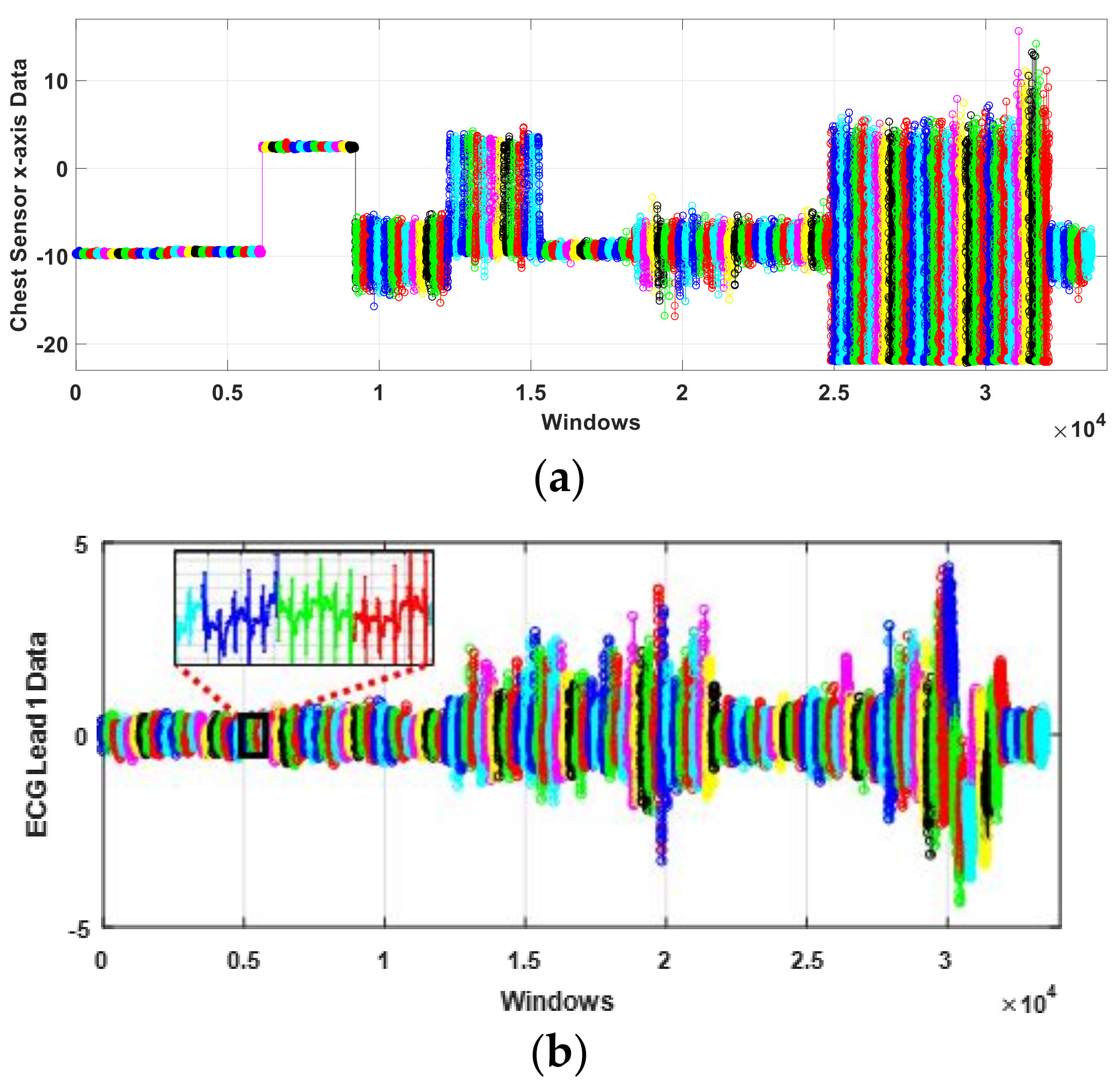
Sliding windows are used to partition the bio-signal into fixed-sized time windows that can be either non-overlapping or overlapping. Overlapping sliding windows have a generalized positive impact on the performance of the proposed HF-SPHR system. Figure 3 demonstrates all of the windows generated for the x-axis of the IMU when it is placed on the chest, and for lead 1 of the ECG.
2.3. IMU-Based Hybrid Feature Extraction
An inertial measurement unit is a mechanized device that is used to monitor and provide data on object-specific force, angular degree [41] and positioning values. It uses a combination of accelerometers, gyroscopes and magnetometers, which consist of x, y, and z axes. After the pre-processing phase is completed, the second phase is to generate hybrid features from each sensor’s processed signal separately. The four major domains of hybrid features employed are statistical non-parametric, entropy-based, wavelet transform, and Mel-frequency cepstral coefficient features. This paper proposes three features for IMU signals: 1D-LBP, state-space correlation entropy (SSCE), and dispersion entropy (DE), which is explained in the sections below. Algorithm 2 (1 SSCE and 2 Dispersion Entropy [42,43,44]) shows the pseudocode for the overall IMU feature extraction.
| Algorithm 2 IMU Feature Abstraction |
 |
2.3.1. 1D Local Binary Pattern
1D-LBP is a non-parametric statistical feature extraction [45] technique. It focuses on the vibration of the signal, and captures the descriptive information representing the relative changes in the IMU signal amplitudes. This feature requires substantially less computational power, and has strong discriminative capabilities.
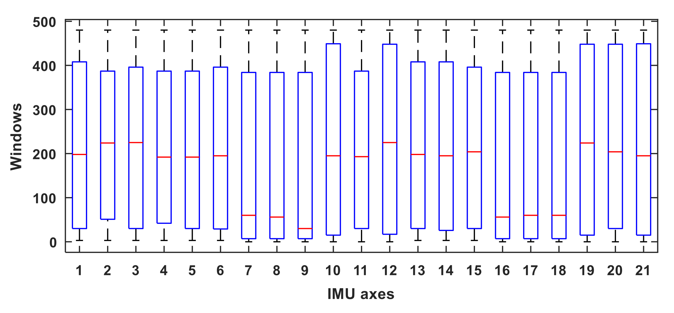
Here in Equation (1), x is the signal window for 1D-LBP, y is the threshold, T represents selected binary values, and n is the number of total values in each selected window. Figure 4 denotes 1D-LBP features for the mHealth dataset. Each IMU axis is represented on the x-axis, whereas the y-axis represents the number of windows. Each box in the figure visually represents the 1D-LBP data for every IMU axis. The central red mark in the box indicates the median, while the bottom and top edges of the box indicate the 25th and 75th percentiles, respectively.
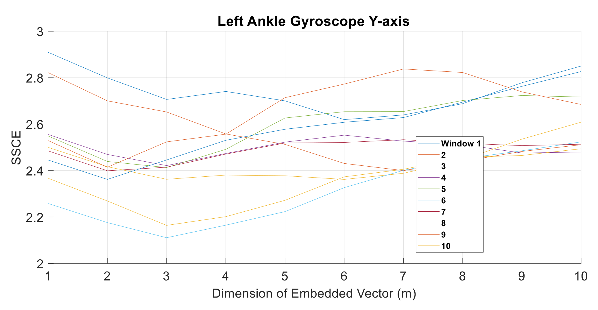
2.3.2. State–Space Correlation Entropy
The data related to the time series can be divided into embedded vectors. The state space covariance matrix captures the correlations of the embedded vectors in a time series. The upper triangular and lower triangular elements of the matrix are identical. The diagonal elements of the matrix capture the autocorrelation of the embedded vectors which are calculated from the probability of the correlations between the embedded vectors (See Figure 5) using Equation (2). The dimension of embedded vector is another important parameter for SSCE, for which, when small, the number of embedded vectors is high.
where Pk is the probability evaluation and n is the number of bins.
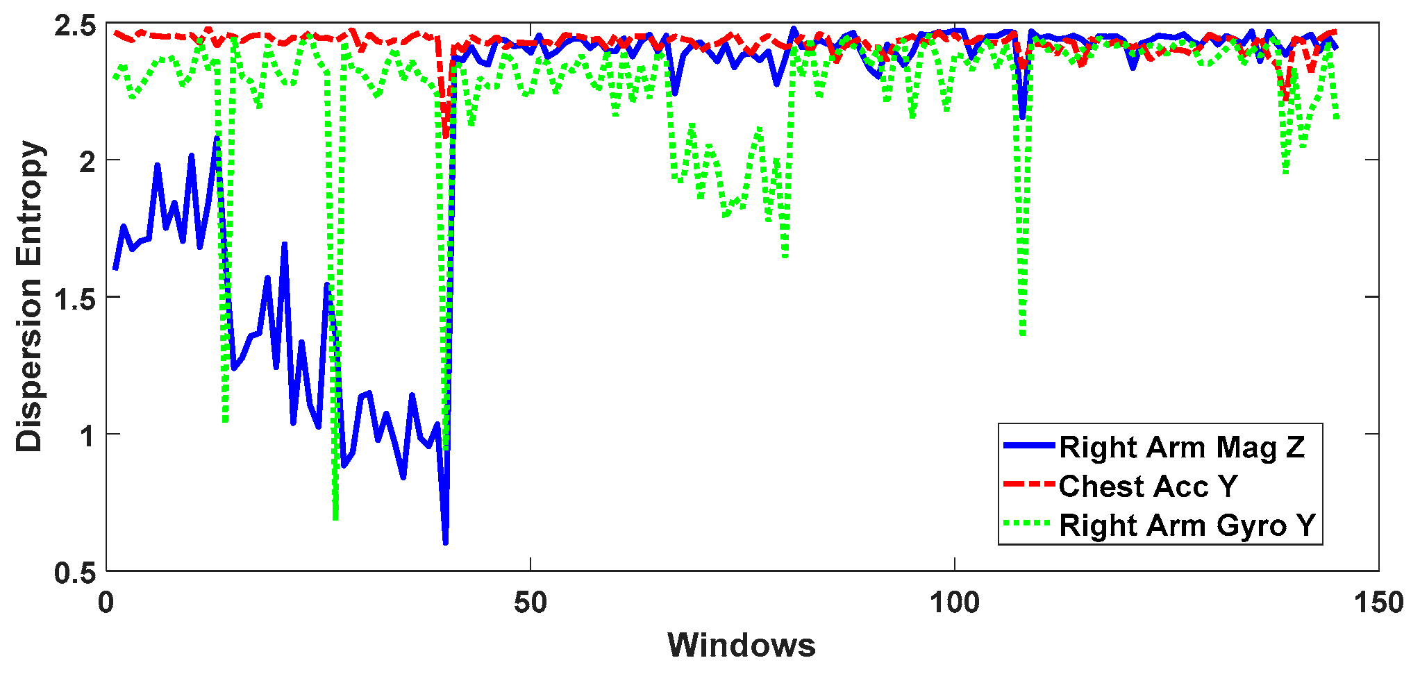
2.3.3. Dispersion Entropy
Dispersion Entropy is used to quantify the regularity of a time series and detect noise bandwidth, simultaneous frequencies, and amplitude changes. As a measure of uncertainty, DE tackles the limitations of permutation entropy and Shannon entropy, including the discrimination of different groups of similar traits with lesser computation time. Dispersion entropy includes four main steps, and they are formulated according to Equation (3);
where, x is the signal, m is the embedding dimension, c is the number of classes, d is the time domain, and is the number of dispersion patterns, computed as in Equation (4). Meanwhile, is the embedding vector, and d is the time delay, as shown in Figure 6.
2.4. ECG-Based Hybrid Feature Extraction
ECG-based features are classified into five types that detect possible heart problems and other abnormalities [46] related to SPHR. These ECG feature extractions are explained in Algorithm 3 (1 MFCC [47,48,49]), which is provided in the section.
| Algorithm 3 ECG Feature Abstraction |
 |
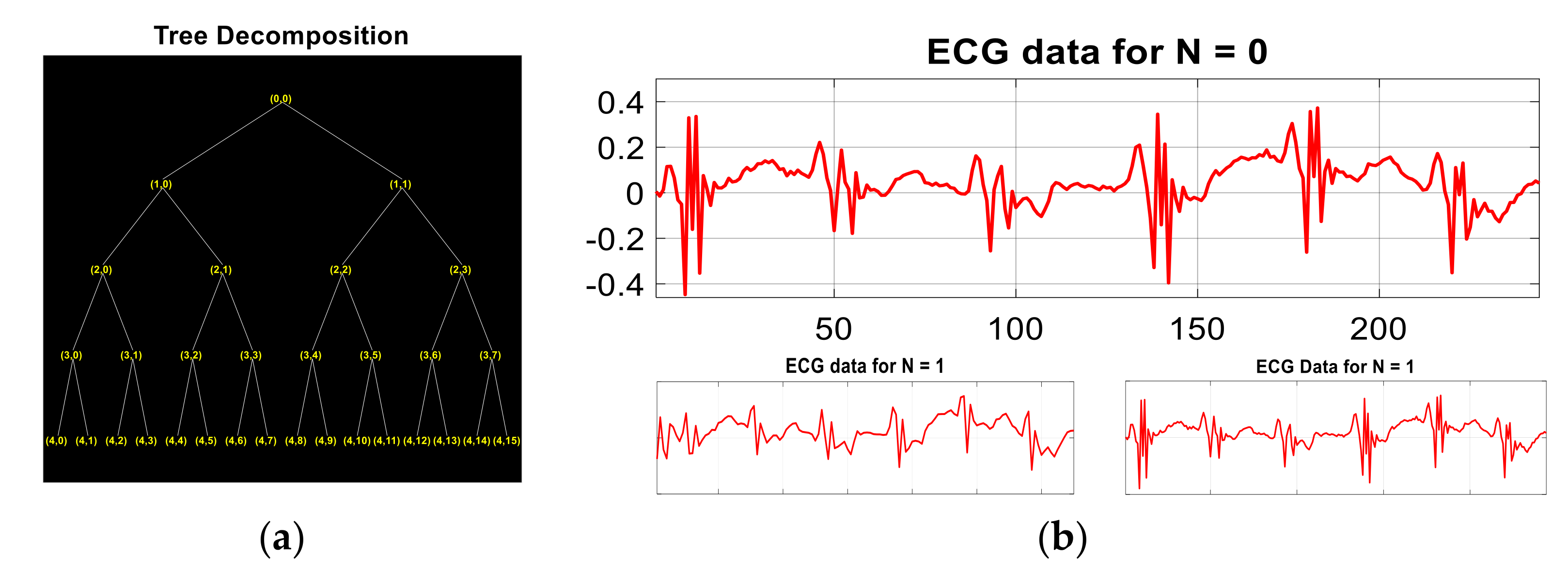
2.4.1. Wavelet Packet Entropy (WPE)
In WPE, the original signal is decomposed into two components—detail coefficients (DCs) and approximation coefficients (ACs)—using a wavelet decomposition tree [50] until the decomposition level is reached. Mathematically, this procedure of decomposition can be defined as in Equation (5):
where h(k) and g(k) are the two filters that are used to obtain ACs/DCs, and represents the reconstruction signals at the ith level and jth node. A decomposition wavelet tree (DWT) is shown using four-level decomposition into ACs and DCs in Figure 7a, whereas a two-level wavelet packet decomposition into AC and DC is presented in Figure 7b.
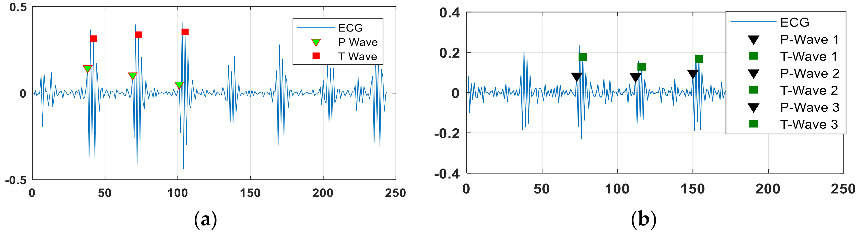
2.4.2. P-Wave and T-Wave Detection
P- and T-wave detection features are used to extract ECG signals using a Q-wave, R-wave, and S-wave (QRS) complex and a Hamilton segmenter algorithm. According to the Hamilton segmenter algorithm, we need to apply a few rules to every cycle, which is called a QRS complex, in an ECG signal. Equations (6) and (7) explain the rules adopted from the algorithm for P-wave and T-wave detection:
where h(x) represents the height of the peak detected, and represents the width of the peak. By using these formulas, we have developed an algorithm, which is presented in Algorithm 3. The samples of the finding of P and T waves from two different activities, like jogging and sitting, are given below in Figure 8. After discovering the QRS complex for each ECG cycle in Figure 8a, the red squares denote the T wave detection, whereas the green triangles represent the P-wave detection for the jogging activity. In Figure 8b, the black triangles symbolize P waves, and the green squares represent T-wave detection for the lying down activity.
2.4.3. Mel-Frequency Cepstral Coefficients
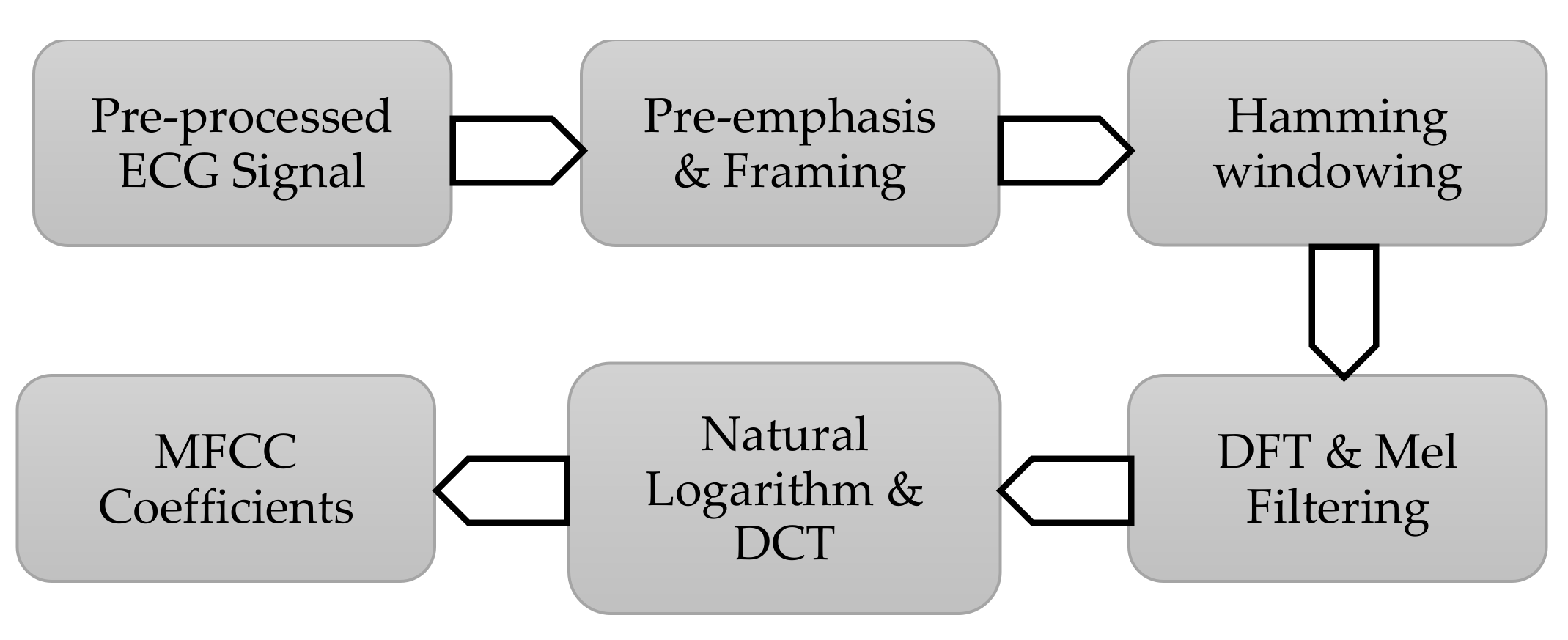
During the MFCC coefficient generation, we initially pre-processed the ECG signal by applying pre-emphasis with α = 0.97. With an analysis frame duration of 3000 ms and a frame shift of 10 ms, the signal is then windowed using hamming and N as 256. Next, in order to take the discrete Fourier transform of the frame, Equation (8) is used, where h(n) is a N sample long analysis window, K is the length of DFT, and si(n) is the periodogram-based power spectral estimate for the frame, which is formulated as:
Meanwhile, Mel filtering, a Natural Logarithm, and DCT are applied (See Figure 9), with the number of Mel filter-bank channels being 20, the number of cepstral coefficients being 12, and the liftering parameter being 22. The filter-banks are created using Equation (9), where m is the number of filters and (f) is the list of m + 2 Mel-spaced frequencies:
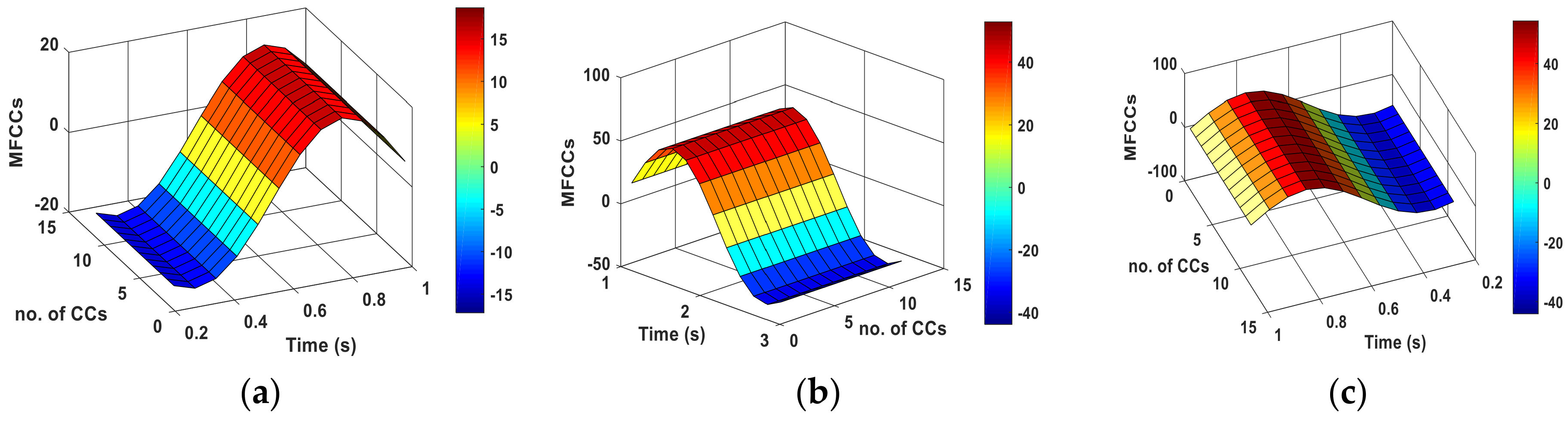
However, in order to calculate the 12 cepstral coefficients, Equation (10) is used, where dt is the coefficient from the t frame, and a typical value for N is 2. Figure 10 represents a few outcomes of MFCC for different activities.
2.4.4. R-Point Detection and R–R Interval
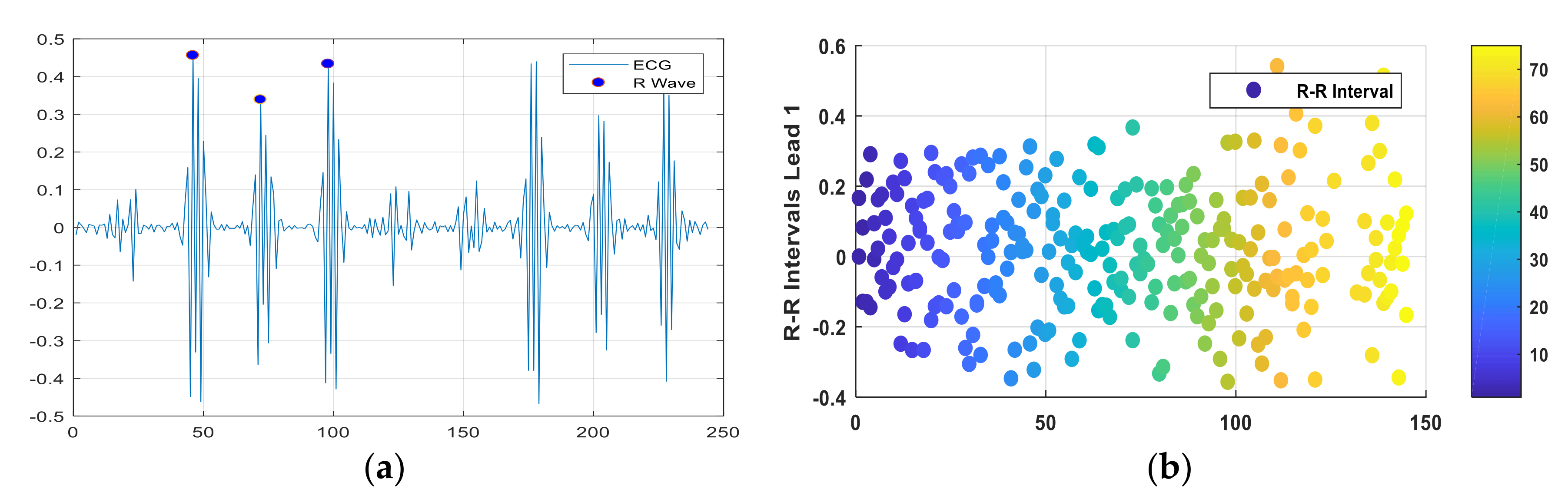
The R-point is the top peak in a QRS complex [51]; therefore, we extracted the R-points first using Equation (11), where is the minimum height peak of a specific signal, and are the width limitations for R peaks. Then, the model calculated the difference between two consecutive R-points in the same window. Such differences provide the R–R Intervals in each window, and have a maximum of 3 R peaks. Here, we have extracted three R-points from each window in order to ensure consistency in the feature extraction and to avoid bias towards a particular activity. In Figure 11a, after finding a QRS complex, the R-points are shown using blue circles, and R–R Intervals are detected and presented in Figure 11b using a scatter plot.
2.5. EMG-Based Hybrid Feature Extraction
EMG is a process that is used to record and assess the electrical activity formed by skeletal muscles. For the EMG feature abstraction process, we used entropy-based features, which include a nonlinear dynamic parameter [52] for the measurement of signal complexity. We used the fuzzy entropy, approximate entropy, and Renyi entropy of orders 2 and 3. Algorithm 4 (1 Fuzzy Entropy [53,54]; 2 Approximate Entropy [55]; 3 Renyi Entropy [56]) in the section explains the implementation of all three types of entropies for the EMG signal.
| Algorithm 4 EMG Feature Abstraction |
 |
2.5.1. Fuzzy Entropy
Fuzzy entropy is the negative natural logarithm of the conditional probability in which two vectors with similar m points remain similar for m + 1 points. Fuzzy entropy measures the regularity of time series more efficiently as:
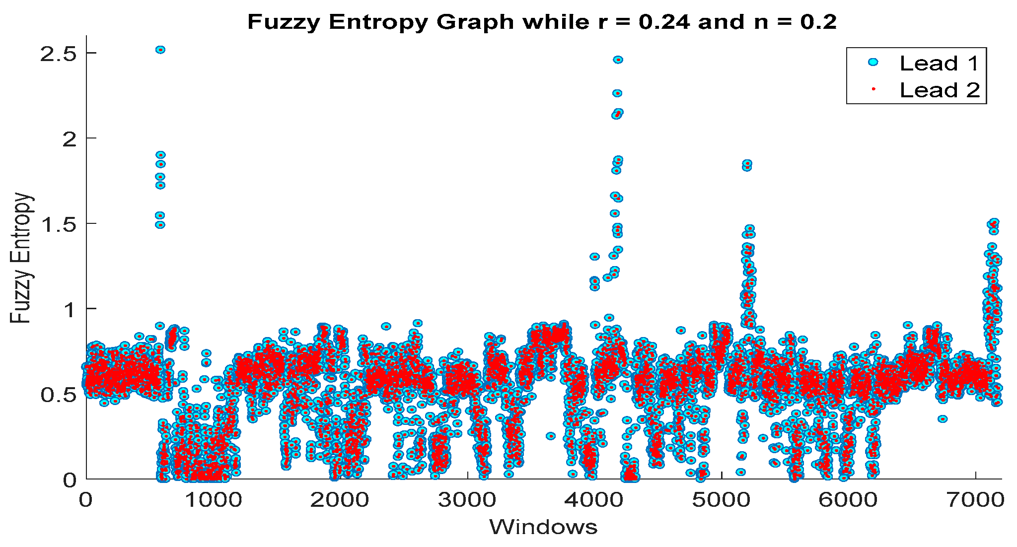
where, in Equations (12)–(14), m is the consecutive vector sequence, n is the gradient, r is the width of the boundary of the exponential function, N is the sample time series, and is the degree of similarity. Following, we used different values for n and r, which leads to a decrease in the standard deviation. Here, we selected r = 0.24 and n = 0.2 for all of the windows of both ECG leads in the HuGaDB dataset, as shown in Figure 12.
2.5.2. Approximate Entropy
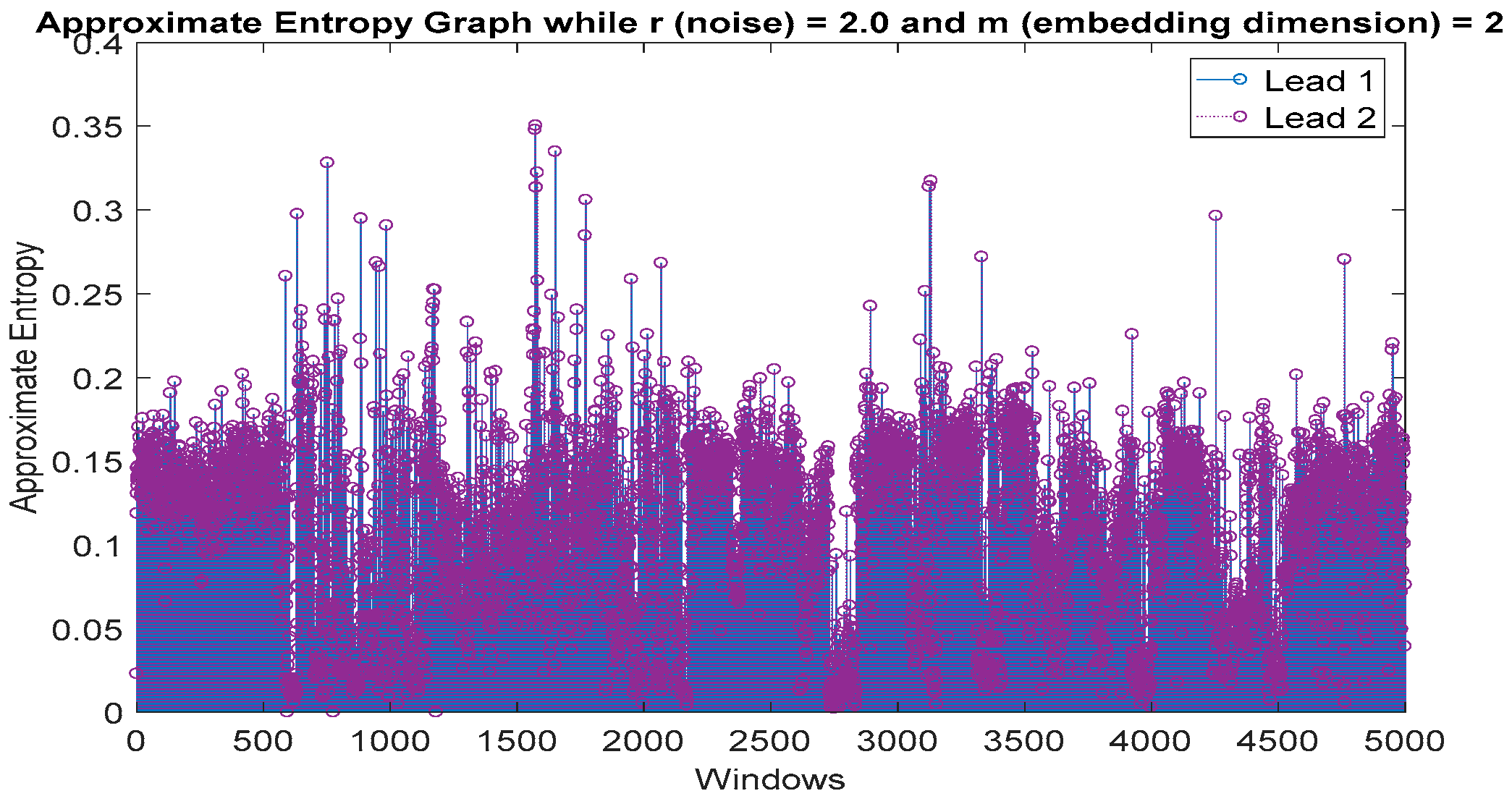
During approximate entropy, we measure the randomness of a series of data without any previous knowledge [57] about the dataset. Equations (15) and (16) show the inner concept of the calculation of approximate entropy, where m is the embedding dimensions and r is the noise filter. We used m = 2 and r = 2.0 for our data. Figure 13 shows the approximate entropy calculated for the EMG leads using the above-mentioned parameters:
2.5.3. Renyi Entropy Order 2 and Order 3
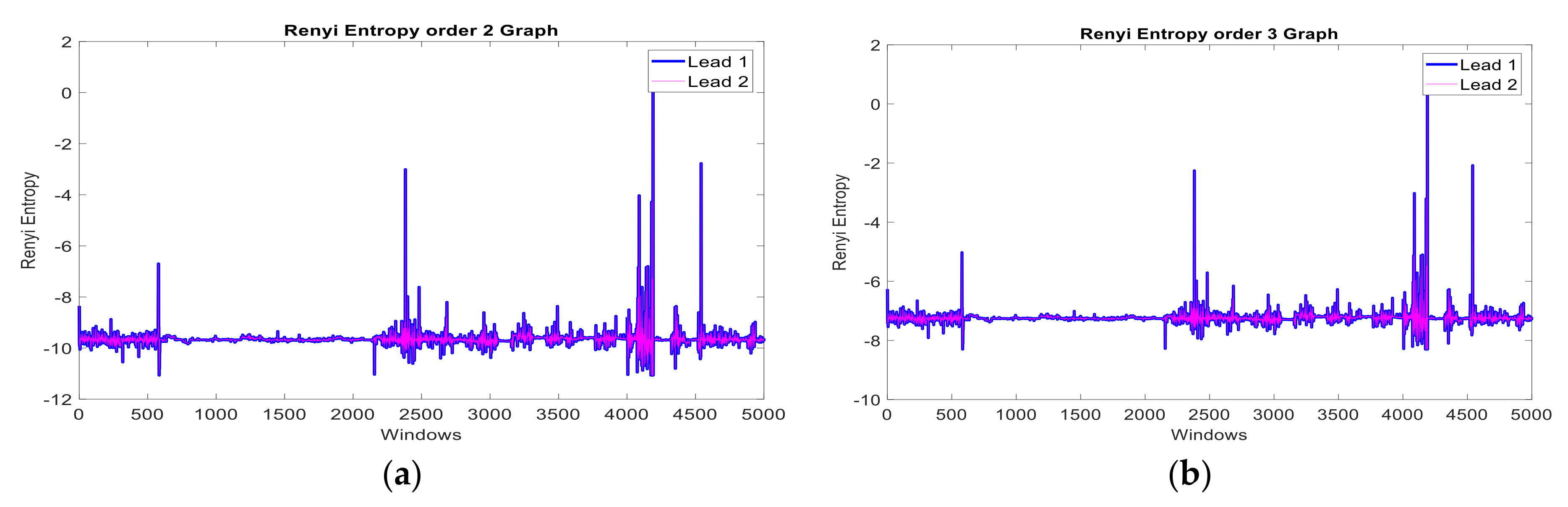
Renyi entropy is the generalization of Shannon’s entropy explained in Equation (18), which preserves the additivity of statistically-independent systems [58,59], and is commonly used for the analysis of biosignals [60]. Equation (17) presents the formula for the calculation of the Renyi entropy for order, where s is the signal sample values, is the order = 2, 3,…, M is the finite number of possible values from s, and p is the probability of each s. Figure 14 shows the Renyi entropy of for the EMG signal leads.
2.6. Feature-to-Feature Fusion
After the separate extraction of the IMU, ECG, and EMG, the model proposes to fuse the hybrid features for each sensor type together, as described in Equations (19)–(21);
Furthermore, in order to obtain more complete global information, the fused features from all three sensors will again be merged together based on time. This type of data fusion is also known as feature in–feature out, where the input and output of the fusion show both features, as shown in Figure 15. Equation (22) shows the formula to fuse the hybrid features from each sensor:
2.7. Feature Reduction: Modified Multi-Layer Sequential Forward Selection
In the feature reduction phase, we eliminate unnecessary features based on a search strategy and an objective function. In search strategies, the algorithms are further categorized into sequential algorithms and randomized algorithms. Similarly, the objective functions are also categorized into filters and wrappers [61]. Dimension reduction not only helps to obtain better results for classification; it can also be used to find those features which act as the best predictors. Here, we proposed a unique algorithm for the feature reduction, designated as modified multi-layer sequential forward selection.
Whitney’s implementation for sequential forward selection (SFS) has been used by many data scientists, and is based on the formula given in Equation (23), where Sd is the feature set of size d, D is the dataset values, and M is the classification model used as KNN. Equation (24) explains how to maintain the monotonicity condition in two subsets of the feature set Sd while J is the condition.
The outdated SFS selected feature sets using a single layer. The MLSFS preserves the features of a signal until the correlation rates for all of the features are established. Furthermore, MLSFS will select the most correlated features captured from the well-defined correlation rates. It achieved better accuracy in feature reduction, and it is presented in Algorithm 5, which is provided in the section.
| Algorithm 5 Multi-layer Sequential Forward Selection algorithm |
 |
2.8. Codebook Generation
In order to encode the resultant fused features, a codebook known as a Gaussian mixture model is used. It is a widely accepted method for representing complex information and feature matching [62] based on an expectation maximization (EM) algorithm. The EM algorithm estimates the unknown parameter sets Θ of probabilistic weights, and helps to find the maximum likelihood function by giving an initial parameter set Θ1 and continuing to apply E and M steps. Then, the EM algorithm generates a sequence {Θ1, Θ2, …, Θm, …} and considers both E and M steps, as in Equations (25) and (26):
where, presents the probability of the jth sample with the kth Gaussian element at the mth iterations along weights , means , and covariance values. Similarly, Gaussian mixture regression provides a way of extracting a single generalized signal from the set of features given. Hence, we can clearly retrieve an analytically smooth signal through regression by encoding the temporal signal features [63] into a mixture of Gaussians. This technique takes each vector of the signals’ GMM as an input of xI and finds the output xO using GMR.
Finally, GMR is considered to provide better results compared to other stochastic approaches because it gives a fast and logical means to restructure the ‘best’ sequence from a Gaussian model. Figure 16 provides a glimpse of GMM–GMR encoded vectors for the HuGaDB and mHealth datasets.
2.9. Deep Belief Network Implementation Using RBMs
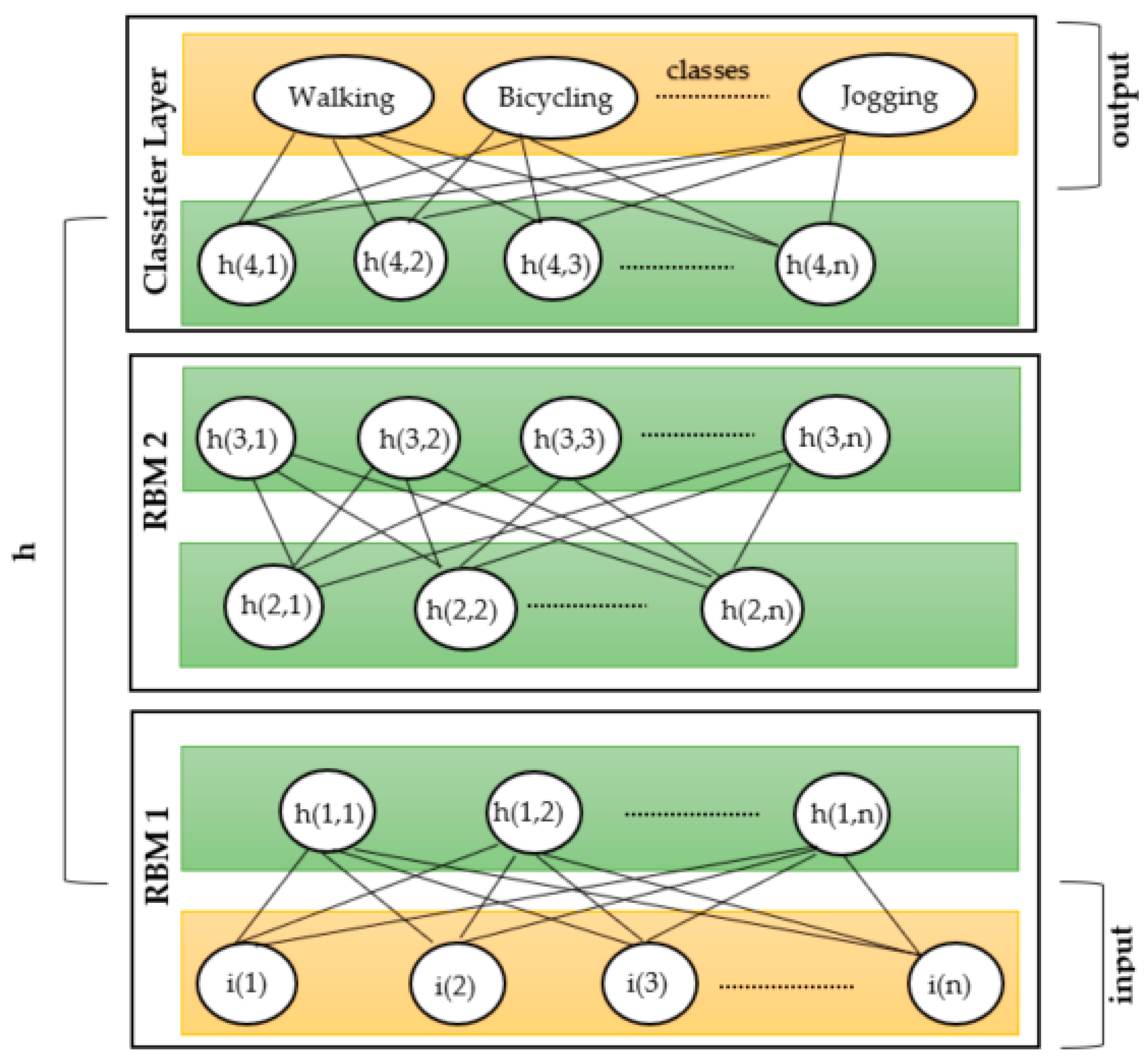
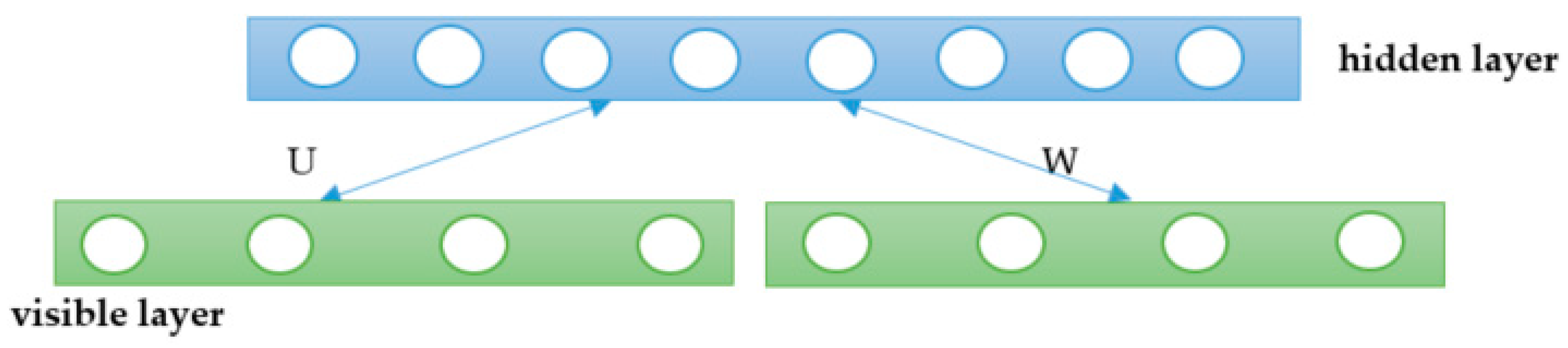
DBNs are multi-layered probabilistic models [64] which consist of multi-parameters for model learning. Each layer contains simple undirected graphs called RBMs. RBM layers are of two types, which are hidden layers and visible layers. The visible layer is the bottom layer, and hidden layers are the top layers. Figure 17 explains the workings of the hidden and visible layers of RBMs. Hidden layers model the probability distribution of the visible variables, and are fully bidirectionally connected with symmetric weights. In RBMs, the layers are not interconnected. The hierarchical processing of stacked RBMs can be used to create a DBN model (See Figure 17). An RBM encodes the joint probability distribution via the energy function, as in Equation (27), in which v is the visible data, h is the hidden data, w is the weight, and = (w, b(v), b(h)). We can write the encoded joint probability as in Equation (28):
These rules are derived to update the initial states, such that every update gives a lower energy state and ultimately settles into equilibrium. Here, in Equations (29) and (30), σ(x) = 1/(1 + exp(−x)), where the sigmoid function is observed as:
In order to train the RBMs, the visible layer is provided with the input data. Here, the learning is to adapt the parameter θ such that the probability distribution in Equation (28) becomes maximally similar to the true values, which means that it will maximize the log-likelihood of each generation of the observed data. A contrastive divergence (CD) algorithm samples the new values for all of the hidden layers in parallel with the current input in order to give a complete sample (vdata, hdata). Furthermore, it generates a sample for the visible layer, and then samples the hidden layer again. Then, we obtain the sample from the model as (vmodel, hmodel). The weights can be updated according to Equation (31).
3. Experimental Performance
In order to evaluate the accomplishment of the DBN classifier [65] for human activity recognition, this paper considered using accuracy, sensitivity, specificity, precision, recall, F-measure and misclassification scores as the performance measures. The accurate classification of the SPHR is called accuracy [66], as expressed in Equation (32). In Equations (32)–(36), TN, TP, FN, and FP represent true negative, true positive, false negative, and false positive, respectively.
Sensitivity measures the proportion of actual positives that are correctly identified, and this is called the true positive rate (TPR). Equation (33) describes the formula used to calculate the sensitivity.
Specificity is defined as the measure of the proportion of negatives that are correctly identified. Equation (34) gives us the formula to measure the specificity, given TN and FP.
Precision is the proportion of true positives correctly identified from total positives. Equation (35) describes the formula for the calculation of precision.
Recall is the proportion of all true positives out of true positives and false negatives. Equation (36) tells us the formula for recall.
where n represents all classes for classification.
The F-measure is a method to combine precision and recall together into a single measure that captures the quality of both performance measures. The misclassification rate can be calculated from the accuracy:
3.1. Datasets Description
In order to appraise the testing/training abilities of our proposed model, we used two public benchmark datasets, i.e., the mHealth dataset [67] from the UCI Machine Learning repository, and the HuGaDB dataset [68] from the GitHub repository.
In the mHealth dataset, there are a total of 12 activities with 24 attributes each. It uses 21 attributes for IMU sensors on the chest, left ankle and right arm, two attributes for the ECG sensor, and one attribute for the labels describing the activity performed. The dataset represents 10 subjects and locomotion activities: standing still, sitting and relaxing, lying down, walking, climbing stairs, waist bending forward, the frontal elevation of arms, knees bending (crouching), cycling, jogging, running, and jumping back and forth. Each subject had all of the above-mentioned sensors attached, with a frequency of 50 Hz.
The second dataset used to evaluate performance was a human gait database. It consists of 12 activities and 39 attributes for each activity. For IMU, there are 36 attributes; for EMG, there are two attributes; and the last attribute is for the activity label. This dataset was collected for 18 subjects with repeated activities. The activities were walking, running, going up, going down, sitting, sitting down, standing up, standing, bicycling, going up by elevator, going down by elevator, and sitting in car. Six IMUs and two EMG sensors were attached to each subject, and a sample rate of 1000 Hz was used.
In our work, the data from all of the subjects is separated with respect to the sensors’ nature, and then preprocessed to remove noise. Finally, the signals were split into windows of 5 s each, with 12 overlapping values. We used the ‘leave-one-subject-out’ (LOSO) [69] cross-validation technique for the training and testing.
3.2. Results Evaluations
The experiment was performed with a laptop, with the specification of the CPU being i7-8550 and the RAM being 24 GB, and a NVIDIA GeForce GTX GPU 2 GB. The programming tool was MATLAB, with multiple frameworks available in the tool and online. For efficient results, the sample data from HuGaDB was sent to the Gaussian mixture models in batches of half the sample length for the walking activity. The model used deep belief network with RBMs of four layers in order to minimize reconstruction errors and set the number of training samples according to the cross-validation. RBMs use CD as a sampling method type. The learning rate for each RBM was set to 0.05, and the model uses discriminative RBMs, as explained in Figure 18.
In the first layer of the RBMs, we set the number of nodes to the number of input variables. The second, third, fourth, and fifth RBM layers had 500, 500, 500, and 1000 nodes. All of the training and testing sample sets from the cross-validation were looked into one after the other in order to see which set performed best. By training and testing the test set, the classification confusion matrix was produced for the mHealth dataset as in Table 1; for the HuGaDB dataset, see Table 2.
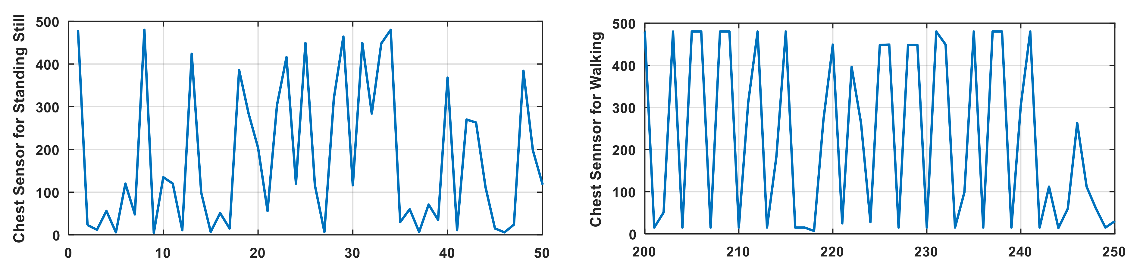
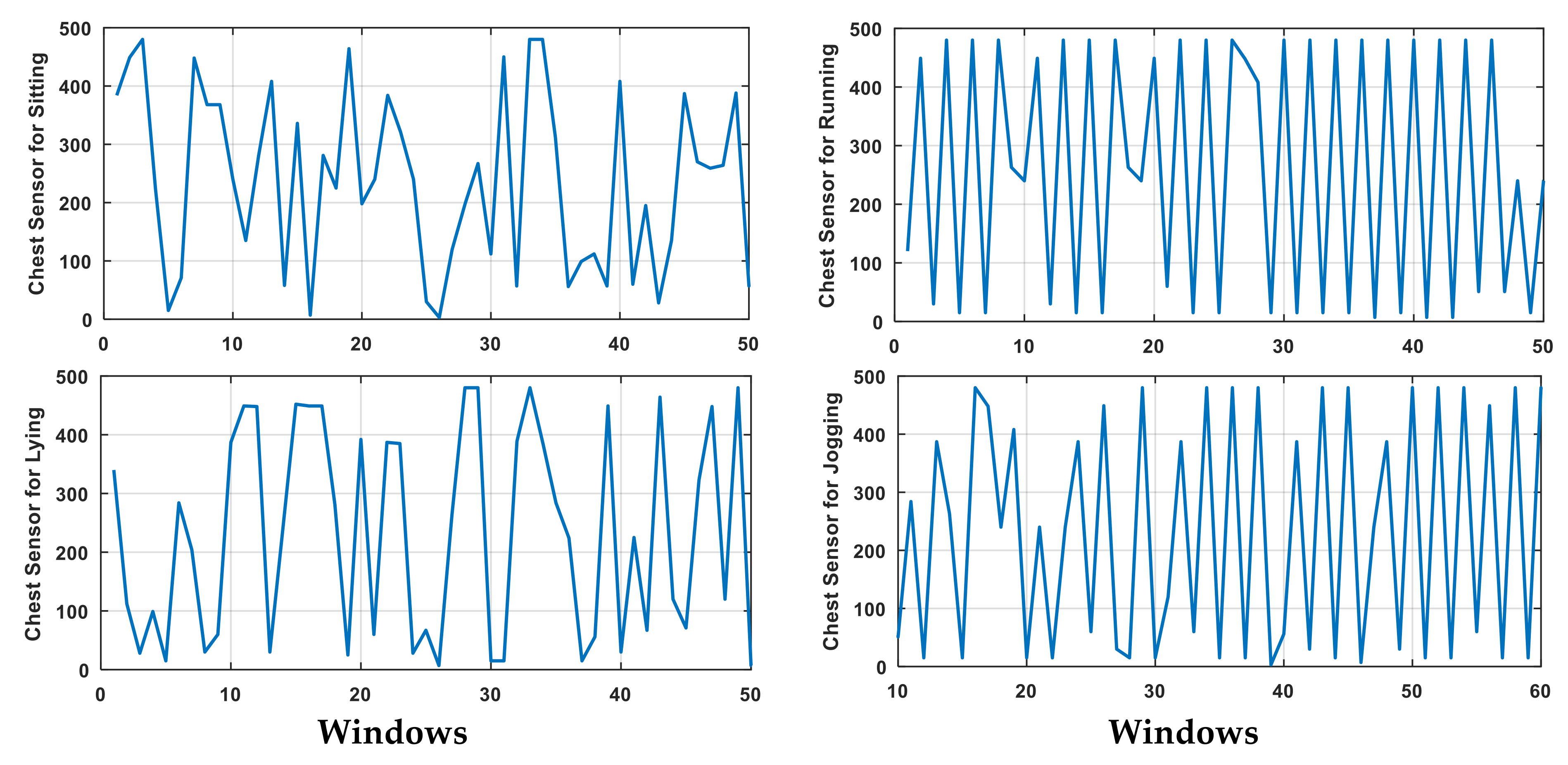
It can be observed from Figure 19 column 1 that there are activities with high altitudes of signal closeness to each other, i.e., standing still, sitting, and lying down. Similarly, the walking, running and jogging signals bear a resemblance to each other in column 2. It is important to notice that our proposed model is able to distinguish between such activities with decent accuracy rates of 93.33% for the mHealth dataset and 92.50% for the HuGaDB datasets.
Comparisons of the sensitivity and specificity are given in Table 3 for the mHealth dataset and Table 4 for the HuGaDB dataset. Table 5 shows the precision, recall, and F-measure for each activity for both datasets.
A comparison between the different layers of the RBMs using the time and number of iterations is presented in Table 6. Parameter tuning [70] is an important step of DBN. Hence, a batch size of 15 samples was used; the weight cost for each node was set to 0.0002, and a maximum of seven epochs for each layer was proposed as the list of parameters [71] being tuned. The reconstruction error for each layer decreases as the RBM moves towards the next layer. The time in seconds is given, and the number of nodes can also be observed.
Table 7 presents the comparative study results using the accuracies for the proposed model and other statistically–well-known classifiers and methodologies i.e., random forest, artificial neural network, ensemble algorithms, Adam based optimization, decision trees, SVM, kNN, and Hampel Estimated. The overall results show that the proposed model achieved better classification results using a deep belief network and discriminative RBMs, which shows a novel contribution for SPHR. The proposed HF-SPHR model has to be assessed and adjusted according to the following challenges:
- In its actual implementation, pattern recognition challenges were faced while the same activity was performed by different individuals.
- Wearable-sensors–based architectures are susceptible to placement changes and other locomotion activities.
We used other state-of-the-art classifier techniques like random forest and AdaBoost for comparison with the proposed DBN and RBM model. Table 8 shows that DBN significantly outperforms other classifiers with regard to its accuracy rate.
4. Discussion
This paper proposed a robust sustainable system with consistency across different challenging datasets; because elderly and disabled individuals [82] stay indoors, two indoor activity-based datasets were used for stability. The proposed HF-SPHR system produced a good quality performance with both datasets, handling problems of varying human activities and a variety of signal shapes due to the incorporation of multiple types of sensors. The actions performed in both datasets are complex, because the movements involved in performing most of the activities are quite similar—namely, jogging, running, walking and standing, sitting, lying-down—as described in Figure 19. However, HF-SPHR remained composed and reliable in recognizing and distinguishing between similar actions due to the robust hybrid features. The proposed system showed high accuracy, specificity, precision, recall, and F-measure rates.
The ECG cycle extraction was challenging due to the similarity in actions like lying-down and sitting. In the feature extraction phase, the QRS complex was identified successfully using a few important ECG peak rules, followed by the extraction of the P wave, T wave, R wave, and R–R Intervals as features of the ECG signals. However, the similarity between some actions caused QRS complex cycles to overlap more significantly with each other in a few instances. For example, in classes such as jogging and running, the QRS complex cycles overlapped at some points. As such, the performance of such actions was been compromised due to the overlapping of the QRS complexes. However, our system offered different domains’ features—namely, WPE and MFCC in hybrid form—to keep the performance at a high level.
5. Conclusions
This paper proposed a robust model for sustainable physical healthcare Pattern Recognition with hybrid feature manipulation and Gaussian mixture models. It also suggested the application of a deep belief network classifier with discriminative RBMs, which automatically extracts features and also reduces the dependence on domain experts. This model achieved excellent recognition results. HF-SPHR can also serve the purpose of a deep learning model that can efficiently and sustainably recognize activities. By introducing the structure of MFCC, entropy and other features, HF-SPHR effectively extracts the raw data from different sensors more comprehensively, extracts more relevant features, and increases the diversity of the feature sets. The experiments also revealed the influence of the HF-SPHR model in terms of accuracy, sensitivity, specificity, precision, recall, and the F-measure. HF-SPHR helped in constructing an ideal human behavior recognition model. It is worth mentioning that the proposed HF-SPHR technique recognized static activities with lower accuracies compared to dynamic activities where further improvements are necessary. It will be of interest to see how the model performs for complex activities.
Author Contributions
Conceptualization, M.J. and M.G.; methodology, M.J., M.G. and A.J.; software, M.J.; validation, M.J. and A.J.; formal analysis, M.G. and K.K.; resources, A.J., M.G. and K.K.; writing—review and editing, M.J., A.J. and K.K.; funding acquisition, A.J. and K.K. All authors have read and agreed to the published version of the manuscript.
Funding
This research was supported by the Basic Science Research Program through the National Research Foundation of Korea (NRF), funded by the Ministry of Education (No. 2018R1D1A1A02085645). Additionally, this work was supported by the Korea Medical Device Development Fund grant funded by the Korea government (the Ministry of Science and ICT, the Ministry of Trade, Industry and Energy, the Ministry of Health & Welfare, the Ministry of Food and Drug Safety) (Project Number: 202012D05-02).
Conflicts of Interest
The authors declare no conflict of interest.
References
- Gochoo, M.; Gochoo, M.; Velusamy, V.; Liu, S.-H.; Bayanduuren, D.; Huang, S.-C. Device-Free Non-Privacy Invasive Classification of Elderly Travel Patterns in A Smart House Using PIR Sensors and DCNN. IEEE Sens. J. 2017, 18, 1287. [Google Scholar] [CrossRef]
- Jalal, A.; Uddin, Z.; Kim, T.-S. Depth video-based human activity recognition system using translation and scaling invariant features for life logging at smart home. IEEE Trans. Consum. Electron. 2012, 58, 863–871. [Google Scholar] [CrossRef]
- Jalal, A.; Kamal, S. Real-time life logging via a depth silhouette-based human activity recognition system for smart home services. In Proceedings of the 2014 11th IEEE International Conference on Advanced Video and Signal Based Surveillance (AVSS), Seoul, Korea, 26–29 August 2014; pp. 74–80. [Google Scholar]
- Dang, L.M.; Min, K.; Wang, H.; Piran, J.; Lee, C.H.; Moon, H. Sensor-based and vision-based human activity recognition: A comprehensive survey. Pattern Recognit. 2020, 108, 107561. [Google Scholar] [CrossRef]
- Kaixuan, C.; Dalin, Z.; Lina, Y.; Bin, G.; Zhiwen, Y.; Yunhao, L. Deep Learning for Sensor-based Human Activity Recogni-tion: Overview, Challenges and Opportunities. J. ACM 2018, 37. [Google Scholar] [CrossRef]
- Shrestha, A.; Mahmood, A. Review of Deep Learning Algorithms and Architectures. IEEE Access 2019, 7, 53040–53065. [Google Scholar] [CrossRef]
- Nweke, H.F.; Teh, Y.W.; Al-Garadi, M.A.; Alo, U.R. Deep learning algorithms for human activity recognition using mobile and wearable sensor networks: State of the art and research challenges. Expert Syst. Appl. 2018, 105, 233–261. [Google Scholar] [CrossRef]
- Tingting, Y.; Junqian, W.; Lintai, W.; Yong, X. Three-stage network for age estimation. CAAI Trans. Intell. Technol. 2019, 4, 122–126. [Google Scholar] [CrossRef]
- Osterland, S.; Weber, J. Analytical analysis of single-stage pressure relief valves. Int. J. Hydromechatron. 2019, 2, 32. [Google Scholar] [CrossRef]
- Wang, J.; Chen, Y.; Hao, S.; Peng, X.; Hu, L. Deep learning for sensor-based activity recognition: A survey. Pattern Recognit. Lett. 2019, 119, 3–11. [Google Scholar] [CrossRef] [Green Version]
- Zhang, S.; Wei, Z.; Nie, J.; Shuang, W.; Wang, S.; Li, Z. A Review on Human Activity Recognition Using Vision-Based Method. J. Healthc. Eng. 2017, 2017, 1–31. [Google Scholar] [CrossRef] [PubMed]
- Jalal, A.; Kamal, S.; Kim, D. A Depth Video Sensor-Based Life-Logging Human Activity Recognition System for Elderly Care in Smart Indoor Environments. Sensors 2014, 14, 11735–11759. [Google Scholar] [CrossRef]
- Espinosa, R.; Ponce, H.; Gutiérrez, S.; Martínez-Villaseñor, L.; Brieva, J.; Moya-Albor, E. A vision-based approach for fall detection using multiple cameras and convolutional neural networks: A case study using the UP-Fall detection dataset. Comput. Biol. Med. 2019, 115, 103520. [Google Scholar] [CrossRef]
- Jalal, A.; Quaid, M.A.K.; Tahir, S.B.U.D.; Kim, K. A Study of Accelerometer and Gyroscope Measurements in Physical Life-Log Activities Detection Systems. Sensors 2020, 20, 6670. [Google Scholar] [CrossRef]
- Yang, X.; Tian, Y. Super Normal Vector for Human Activity Recognition with Depth Cameras. IEEE Trans. Pattern Anal. Mach. Intell. 2016, 39, 1028–1039. [Google Scholar] [CrossRef] [PubMed]
- Jalal, A.; Khalid, N.; Kim, K. Automatic Recognition of Human Interaction via Hybrid Descriptors and Maximum Entropy Markov Model Using Depth Sensors. Entropy 2020, 22, 817. [Google Scholar] [CrossRef] [PubMed]
- Mahmood, M.; Jalal, A.; Kim, K. WHITE STAG model: Wise human interaction tracking and estimation (WHITE) using spatio-temporal and angular-geometric (STAG) descriptors. Multimed. Tools Appl. 2020, 79, 6919–6950. [Google Scholar] [CrossRef]
- Jalal, A.; Kim, Y.-H.; Kim, Y.-J.; Kamal, S.; Kim, D. Robust human activity recognition from depth video using spatiotemporal multi-fused features. Pattern Recognit. 2017, 61, 295–308. [Google Scholar] [CrossRef]
- Irvine, N.; Nugent, C.; Zhang, S.; Wang, H.; Ng, W.W.Y. Neural Network Ensembles for Sensor-Based Human Activity Recognition Within Smart Environments. Sensors 2019, 20, 216. [Google Scholar] [CrossRef] [Green Version]
- Xi, X.; Tang, M.; Miran, S.M.; Miran, S.M. Evaluation of Feature Extraction and Recognition for Activity Monitoring and Fall Detection Based on Wearable sEMG Sensors. Sensors 2017, 17, 1229. [Google Scholar] [CrossRef] [PubMed]
- Wijekoon, A.; Wiratunga, N.; Sani, S.; Cooper, K. A knowledge-light approach to personalised and open-ended human activity recognition. Knowl. Based Syst. 2020, 192, 105651. [Google Scholar] [CrossRef]
- Quaid, M.A.K.; Jalal, A. Wearable sensors based human behavioral pattern recognition using statistical features and reweighted genetic algorithm. Multimed. Tools Appl. 2020, 79, 6061–6083. [Google Scholar] [CrossRef]
- Tahir, S.B.U.D.; Jalal, A.; Kim, K. Wearable Inertial Sensors for Daily Activity Analysis Based on Adam Optimization and the Maximum Entropy Markov Model. Entropy 2020, 22, 579. [Google Scholar] [CrossRef]
- Sueur, C.; Jeantet, L.; Chevallier, D.; Bergouignan, A.; Sueur, C. A Lean and Performant Hierarchical Model for Human Activity Recognition Using Body-Mounted Sensors. Sensors 2020, 20, 3090. [Google Scholar] [CrossRef]
- Badawi, A.A.; Al-Kabbany, A.; Shaban, H.A. Sensor Type, Axis, and Position-Based Fusion and Feature Selection for Multimodal Human Daily Activity Recognition in Wearable Body Sensor Networks. J. Healthc. Eng. 2020, 2020, 1–14. [Google Scholar] [CrossRef] [PubMed]
- Shokri, M.; Tavakoli, K. A Review on the Artificial Neural Network Approach to Analysis and Prediction of Seismic Damage in Infrastructure. Int. J. Hydromechatron. 2019, 1, 178–196. [Google Scholar] [CrossRef]
- Ahmed, A.; Jalal, A.; Kim, K. A Novel Statistical Method for Scene Classification Based on Multi-Object Categorization and Logistic Regression. Sensors 2020, 20, 3871. [Google Scholar] [CrossRef] [PubMed]
- Susan, S.; Agrawal, P.; Mittal, M.; Bansal, S. New shape descriptor in the context of edge continuity. CAAI Trans. Intell. Technol. 2019, 4, 101–109. [Google Scholar] [CrossRef]
- Guido, R.C. A tutorial review on entropy-based handcrafted feature extraction for information fusion. Inf. Fusion 2018, 41, 161–175. [Google Scholar] [CrossRef]
- Mallat, S. A theory for multiresolution signal decomposition: The wavelet representation. IEEE Trans. Pattern Anal. Mach. Intell. 1989, 11, 674–693. [Google Scholar] [CrossRef] [Green Version]
- Bruce, L.; Koger, C.; Li, J. Dimensionality reduction of hyperspectral data using discrete wavelet transform feature extraction. IEEE Trans. Geosci. Remote Sens. 2002, 40, 2331–2338. [Google Scholar] [CrossRef]
- Jalal, A.; Batool, M.; Kim, K. Stochastic Recognition of Physical Activity and Healthcare Using Tri-Axial Inertial Wearable Sensors. Appl. Sci. 2020, 10, 7122. [Google Scholar] [CrossRef]
- Yusuf, S.A.A.; Hidayat, R. MFCC Feature Extraction and KNN Classification in ECG Signals. In Proceedings of the 2019 6th International Conference on Information Technology, Computer and Electrical Engineering (ICITACEE), Semarang, Indonesia, 26–27 September 2019; pp. 1–5. [Google Scholar]
- Jalal, A.; Quaid, M.A.K.; Hasan, A.S. Wearable Sensor-Based Human Behavior Understanding and Recognition in Daily Life for Smart Environments. In Proceedings of the 2018 International Conference on Frontiers of Information Technology (FIT), Islamabad, Pakistan, 17–19 December 2018; pp. 105–110. [Google Scholar]
- Javeed, M.; Jalal, A.; Kim, K. Wearable Sensors based Exertion Recognition using Statistical Features and Random Forest for Physical Healthcare Monitoring. In Proceedings of the 18th International Bhurban Conference on Applied Sciences and Technology (IBCAST), Islamabad, Pakistan, 12–16 January 2021. [Google Scholar]
- Pervaiz, M.; Jalal, A.; Kim, K. Hybrid Algorithm for Multi People Counting and Tracking for Smart Surveillance. In Proceedings of the 18th International Bhurban Conference on Applied Sciences and Technology (IBCAST), Islamabad, Pakistan, 12–16 January 2021. [Google Scholar]
- Khalid, N.; Gochoo, M.; Jalal, A.; Kim, K. Modeling Two-Person Segmentation and Locomotion for Stereoscopic Action Identification: A Sustainable Video Surveillance System. Sustainability 2021, 13, 970. [Google Scholar] [CrossRef]
- Tahir, S.B.; Jalal, A.; Kim, K. IMU Sensor Based Automatic-Features Descriptor for Healthcare Patient’s Daily Life-log Recog-nition. In Proceedings of the 18th International Bhurban Conference on Applied Sciences and Technology (IBCAST), Islamabad, Pakistan, 12–16 January 2021. [Google Scholar]
- Jalal, A.; Batool, M.; ud din Tahir, S.B. Markerless Sensors for Physical Health Monitoring System Using ECG and GMM Feature Extraction. In Proceedings of the 18th International Bhurban Conference on Applied Sciences and Technology (IBCAST), Islamabad, Pakistan, 12–16 January 2021. [Google Scholar]
- Ahmed, A.; Jalal, A.; Rafique, A.A. Salient Segmentation based Object Detection and Recognition using Hybrid Genetic Transform. In Proceedings of the 2019 International Conference on Applied and Engineering Mathematics (ICAEM), Taxila, Pakistan, 27–29 August 2019; pp. 203–208. [Google Scholar]
- Jalal, A.; Sarif, N.; Kim, J.T.; Kim, T.-S. Human Activity Recognition via Recognized Body Parts of Human Depth Silhouettes for Residents Monitoring Services at Smart Home. Indoor Built Environ. 2012, 22, 271–279. [Google Scholar] [CrossRef]
- Rafique, A.A.; Jalal, A.; Kim, K. Automated Sustainable Multi-Object Segmentation and Recognition via Modified Sampling Consensus and Kernel Sliding Perceptron. Symmetry 2020, 12, 1928. [Google Scholar] [CrossRef]
- Rostaghi, M.; Azami, H. Dispersion Entropy: A Measure for Time-Series Analysis. IEEE Signal Process. Lett. 2016, 23, 610–614. [Google Scholar] [CrossRef]
- Azami, H.; Rostaghi, M.; Abásolo, D.E.; Escudero, J. Refined Composite Multiscale Dispersion Entropy and its Application to Biomedical Signals. IEEE Trans. Biomed. Eng. 2017, 64, 2872–2879. [Google Scholar] [CrossRef] [Green Version]
- Abdul, Z.K.; Al-Talabani, A.; Abdulrahman, A.O. A New Feature Extraction Technique Based on 1D Local Binary Pattern for Gear Fault Detection. Shock. Vib. 2016, 2016, 1–6. [Google Scholar] [CrossRef] [Green Version]
- Turnip, A.; Kusumandari, D.E.; Wijaya, C.; Turnip, M.; Sitompul, E. Extraction of P and T Waves from Electrocardiogram Signals with Modified Hamilton Algorithm. In Proceedings of the International Conference on Sustainable Engineering and Creative Computing (ICSECC), Bandung, Indonesia, 20–22 August 2019; pp. 58–62. [Google Scholar] [CrossRef]
- Young, S.; Evermann, G.; Gales, M.; Hain, T.; Kershaw, D.; Liu, X.; Moore, G.; Odell, J.; Ollason, D.; Povey, D.; et al. The HTK Book (for HTK Version 3.4.1). Engineering Department, Cambridge University. Available online: http://htk.eng.cam.ac.uk (accessed on 19 November 2020).
- Ellis, D. Reproducing the Feature Outputs of Common Programs Using Matlab and melfcc.m. 2005. Available online: http://labrosa.ee.columbia.edu/matlab/rastamat/mfccs.html (accessed on 31 January 2021).
- Jalal, A.; Kamal, S.; Kim, D.-S. Detecting Complex 3D Human Motions with Body Model Low-Rank Representation for Real-Time Smart Activity Monitoring System. KSII Trans. Internet Inf. Syst. 2018, 12, 1189–1204. [Google Scholar] [CrossRef] [Green Version]
- Jalal, A.; Quaid, M.A.K.; Sidduqi, M.A. A Triaxial acceleration-based human motion detection for ambient smart home sys-tem. In Proceedings of the 2019 16th International Bhurban Conference on Applied Sciences and Technology (IBCAST), Islamabad, Pakistan, 8–12 January 2019; pp. 353–358. [Google Scholar]
- Jalal, A.; Quaid, M.A.K.; Kim, K. A Wrist Worn Acceleration Based Human Motion Analysis and Classification for Ambient Smart Home System. J. Electron. Eng. Technol. 2019, 14, 1733–1739. [Google Scholar] [CrossRef]
- Ahmed, A.; Jalal, A.; Kim, K. Region and Decision Tree-Based Segmentations for Multi-Objects Detection and Classification in Outdoor Scenes. In Proceedings of the 2019 International Conference on Frontiers of Information Technology (FIT), Islamabad, Pakistan, 16–18 December 2019; pp. 209–2095. [Google Scholar]
- Azami, H.; Fernández, A.; Escudero, J. Refined multiscale fuzzy entropy based on standard deviation for biomedical signal analysis. Med. Biol. Eng. Comput. 2017, 55, 2037–2052. [Google Scholar] [CrossRef] [PubMed]
- Chen, W.; Wang, Z.; Xie, H.; Yu, W. Characterization of Surface EMG Signal Based on Fuzzy Entropy. IEEE Trans. Neural Syst. Rehabil. Eng. 2007, 15, 266–272. [Google Scholar] [CrossRef]
- Pincus, S.M.; Gladstone, I.M.; Ehrenkranz, R.A. A regularity statistic for medical data analysis. J. Clin. Monit. 1991, 7, 335–345. [Google Scholar] [CrossRef] [PubMed]
- Wenye, G. Shannon and Non-Extensive Entropy. MATLAB Central File Exchange. Available online: https://www.mathworks.com/matlabcentral/fileexchange/18133-shannon-and-non-extensive-entropy (accessed on 6 August 2020).
- Batool, M.; Jalal, A.; Kim, K. Telemonitoring of Daily Activity Using Accelerometer and Gyroscope in Smart Home Envi-ronments. J. Electr. Eng. Technol. 2020, 15, 2801–2809. [Google Scholar] [CrossRef]
- Jalal, A.; Uddin, Z.; Kim, J.T.; Kim, T.-S. Recognition of Human Home Activities via Depth Silhouettes and ℜ Transformation for Smart Homes. Indoor Built Environ. 2011, 21, 184–190. [Google Scholar] [CrossRef]
- Jalal, A.; Kim, Y. Dense depth maps-based human pose tracking and recognition in dynamic scenes using ridge data. In Proceedings of the 2014 11th IEEE International Conference on Advanced Video and Signal Based Surveillance (AVSS), Seoul, Korea, 26–29 August 2014; pp. 119–124. [Google Scholar]
- Vranković, A.; Lerga, J.; Saulig, N. A novel approach to extracting useful information from noisy TFDs using 2D local entropy measures. EURASIP J. Adv. Signal Process. 2020, 2020, 1–19. [Google Scholar] [CrossRef]
- Jalal, A.; Lee, S.; Kim, J.T.; Kim, T.-S. Human Activity Recognition via the Features of Labeled Depth Body Parts. In Lecture Notes in Computer Science (Including Subseries Lecture Notes in Artificial Intelligence and Lecture Notes in Bioinformatics); Springer: Berlin/Heidelberg, Germany, 2012; pp. 246–249. [Google Scholar]
- Jalal, A.; Kamal, S.; Kim, D. Shape and Motion Features Approach for Activity Tracking and Recognition from Kinect Video Camera. In Proceedings of the 2015 IEEE 29th International Conference on Advanced Information Networking and Applications Workshops, Gwangju, Korea, 25–27 March 2015; pp. 445–450. [Google Scholar]
- Jalal, A.; Kamal, S.; Kim, D. Depth silhouettes context: A new robust feature for human tracking and activity recognition based on embedded HMMs. In Proceedings of the 2015 12th International Conference on Ubiquitous Robots and Ambient Intelligence (URAI), Goyang City, Korea, 28–30 October 2015; pp. 294–299. [Google Scholar]
- O’Connor, P.; Neil, D.; Liu, S.-C.; Delbruck, T.; Pfeiffer, M. Real-time classification and sensor fusion with a spiking deep belief network. Front. Neurosci. 2013, 7, 178. [Google Scholar] [CrossRef] [PubMed] [Green Version]
- Keyvanrad, M.A.; Homayounpour, M. A brief survey on deep belief networks and introducing a new object oriented MATLAB toolbox (DeeBNet). arXiv 2014, arXiv:1408.3264. [Google Scholar]
- Akhter, I.; Jalal, A.; Kim, K. Pose Estimation and Detection for Event Recognition Using Sense-Aware Features and Ada-Boost Classifier. In Proceedings of the 18th International Bhurban Conference on Applied Sciences and Technology (IBCAST), Islamabad, Pakistan, 12–16 January 2021. [Google Scholar]
- Banos, O.; Garcia, R.; Holgado-Terriza, J.A.; Damas, M.; Pomares, H.; Rojas, I.; Saez, A.; Villalonga, C. mHealthDroid: A Novel Framework for Agile Development of Mobile Health Applications. In Ambient Assisted Living and Daily Activities. IWAAL 2014. Lecture Notes in Computer Science; Pecchia, L., Chen, L.L., Nugent, C., Bravo, J., Eds.; Springer: Cham, Switzerland, 2020; Volume 8868, pp. 91–98. [Google Scholar]
- Chereshnev, R.; Kertész-Farkas, A. HuGaDB: Human Gait Database for Activity Recognition from Wearable Inertial Sensor Networks. Min. Data Financ. Appl. 2018, 131–141. [Google Scholar] [CrossRef] [Green Version]
- Jalal, A.; Akhter, I.; Kim, K. Human Posture Estimation and Sustainable Events Classification via Pseudo-2D Stick Model and K-ary Tree Hashing. Sustainability 2020, 12, 9814. [Google Scholar] [CrossRef]
- Zhu, C.; Miao, D. Influence of kernel clustering on an RBFN. CAAI Trans. Intell. Technol. 2019, 4, 255–260. [Google Scholar] [CrossRef]
- Wiens, T. Engine Speed Reduction for Hydraulic Machinery Using Predictive Algorithms. Int. J. Hydromechatron. 2019, 2, 16–31. [Google Scholar] [CrossRef]
- Abedin, A.; Motlagh, F.; Shi, Q.; Rezatofighi, H.; Ranasinghe, D. Towards deep clustering of human activities from wearables. In Proceedings of the 2020 International Symposium on Wearable Computers (ISWC ’20). Association for Computing Machinery, New York, NY, USA, 12–17 September 2020; pp. 1–6. [Google Scholar] [CrossRef]
- Fang, B.; Zhou, Q.; Sun, F.; Shan, J.; Wang, M.; Xiang, C.; Zhang, Q. Gait Neural Network for Human-Exoskeleton Interaction. Front. Neurorobot. 2020, 14, 58. [Google Scholar] [CrossRef]
- Maitre, J.; Bouchard, K.; Gaboury, S. Classification models for data fusion in human activity recognition. In Proceedings of the 6th EAI International Conference on Smart Objects and Technologies for Social Good, Antwerp, Belgium, 14–16 September 2020; ACM: New York, NY, USA, 2020; pp. 72–77. [Google Scholar]
- Rasnayaka, S.; Saha, S.; Sim, T. Making the most of what you have! Profiling biometric authentication on mobile devices. In Proceedings of the 2019 International Conference on Biometrics (ICB), Crete, Greece, 4–7 June 2019; pp. 1–7. [Google Scholar] [CrossRef]
- O’Halloran, J.; Curry, E. A comparison of deep learning models in human activity recognition and behavioral prediction on the MHEALTH dataset. In Proceedings of the 27th AIAI Irish conference on Artificial Intelligence and Cognitive Science (AICS), Galway, Ireland, 5–6 December 2019; NUI: Galway, Ireland, 2019. [Google Scholar]
- Sun, Y.; Yang, G.-Z.; Lo, B. An artificial neural network framework for lower limb motion signal estimation with foot-mounted inertial sensors. In Proceedings of the 2018 IEEE 15th International Conference on Wearable and Implantable Body Sensor Networks (BSN), Las Vegas, NV, USA, 4–7 March 2018; pp. 132–135. [Google Scholar]
- Masum, A.K.M.; Hossain, M.E.; Humayra, A.; Islam, S.; Barua, A.; Alam, G.R. A Statistical and Deep Learning Approach for Human Activity Recognition. In Proceedings of the 2019 3rd International Conference on Trends in Electronics and Informatics (ICOEI), Tirunelveli, India, 23–25 April 2019; pp. 1332–1337. [Google Scholar]
- Kumari, G.; Chakraborty, J.; Nandy, A. Effect of Reduced Dimensionality on Deep learning for Human Activity Recognition. In Proceedings of the 2020 11th International Conference on Computing, Communication and Networking Technologies (ICCCNT), Kharagpur, India, 1–3 July 2020; pp. 1–7. [Google Scholar]
- Ha, S.; Choi, S. Convolutional neural networks for human activity recognition using multiple accelerometer and gyroscope sensors. In Proceedings of the 2016 International Joint Conference on Neural Networks (IJCNN), Vancouver, BC, Canada, 24–29 July 2016; pp. 381–388. [Google Scholar]
- Guo, H.; Chen, L.; Peng, L.; Chen, G. Wearable sensor based multimodal human activity recognition exploiting the diver-sity of classifier ensemble. In Proceedings of the 2016 ACM International Joint Conference on Pervasive and Ubiquitous Computing, Heidelberg, Germany, 12–16 September 2016. [Google Scholar]
- Jalal, A.; Batool, M.; Kim, K. Sustainable Wearable System: Human Behavior Modeling for Life-Logging Activities Using K-Ary Tree Hashing Classifier. Sustainability 2020, 12, 10324. [Google Scholar] [CrossRef]
Figure 1.
System architecture of the proposed HF-SPHR model.

Figure 2.
Original and filtered sensor signals; (a) notch filtered data for ECG, (b) median filtered data for IMU, and (c) moving average filtered data for EMG.
Figure 2.
Original and filtered sensor signals; (a) notch filtered data for ECG, (b) median filtered data for IMU, and (c) moving average filtered data for EMG.

Figure 3.
Signal segmentation showing, (a) the windows for the IMU placed on the chest, and (b) the windows for lead 1 of the ECG.
Figure 3.
Signal segmentation showing, (a) the windows for the IMU placed on the chest, and (b) the windows for lead 1 of the ECG.

Figure 4.
Box plot of the 1D-LBP feature for all of the IMU sensors’ axes in the mHealth dataset.

Figure 5.
State-Space Correlation Entropy for each of the given 10 dimensions and windows.

Figure 6.
1D plot of the dispersion entropy feature extraction for the IMU device.

Figure 7.
Wavelet Transform feature: (a) Wavelet Packet Decomposition Tree; (b) a Wavelet Packet decomposition Tree for an ECG with two-level wavelet packet decomposition.
Figure 7.
Wavelet Transform feature: (a) Wavelet Packet Decomposition Tree; (b) a Wavelet Packet decomposition Tree for an ECG with two-level wavelet packet decomposition.

Figure 8.
P–Wave and T–Wave Detection features for (a) jogging and (b) lying down activities.

Figure 9.
MFCC process overview.

Figure 10.
MFCC features extracted for (a) jumping forward and backward, (b) standing still and (c) walking activities.
Figure 10.
MFCC features extracted for (a) jumping forward and backward, (b) standing still and (c) walking activities.

Figure 11.
(a) R–Point Detection of a standing still activity, and (b) R–R Intervals representation with respect to the windows for the ECG.
Figure 11.
(a) R–Point Detection of a standing still activity, and (b) R–R Intervals representation with respect to the windows for the ECG.

Figure 12.
Fuzzy Entropy features extracted for EMG lead 1 and lead 2 for the HuGaDB dataset.

Figure 13.
Approximate Entropy feature Extraction using r = 2.0 and m = 2.

Figure 14.
Renyi entropy feature extraction for (a) order 2 and (b) order 3.

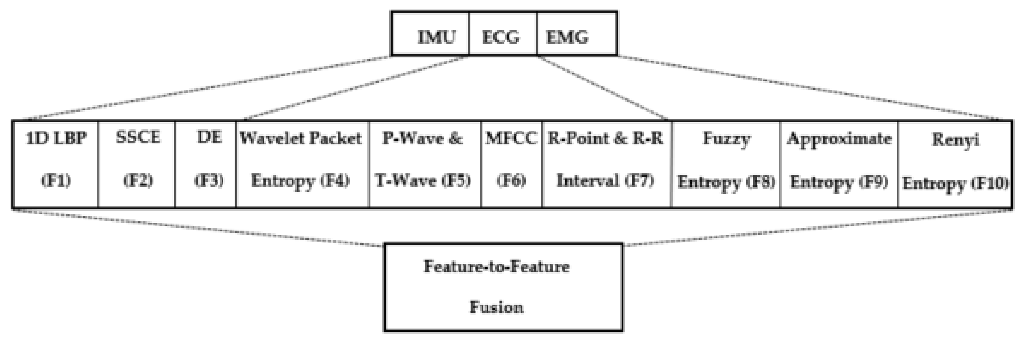
Figure 15.
Proposed feature–to–feature fusion concept.

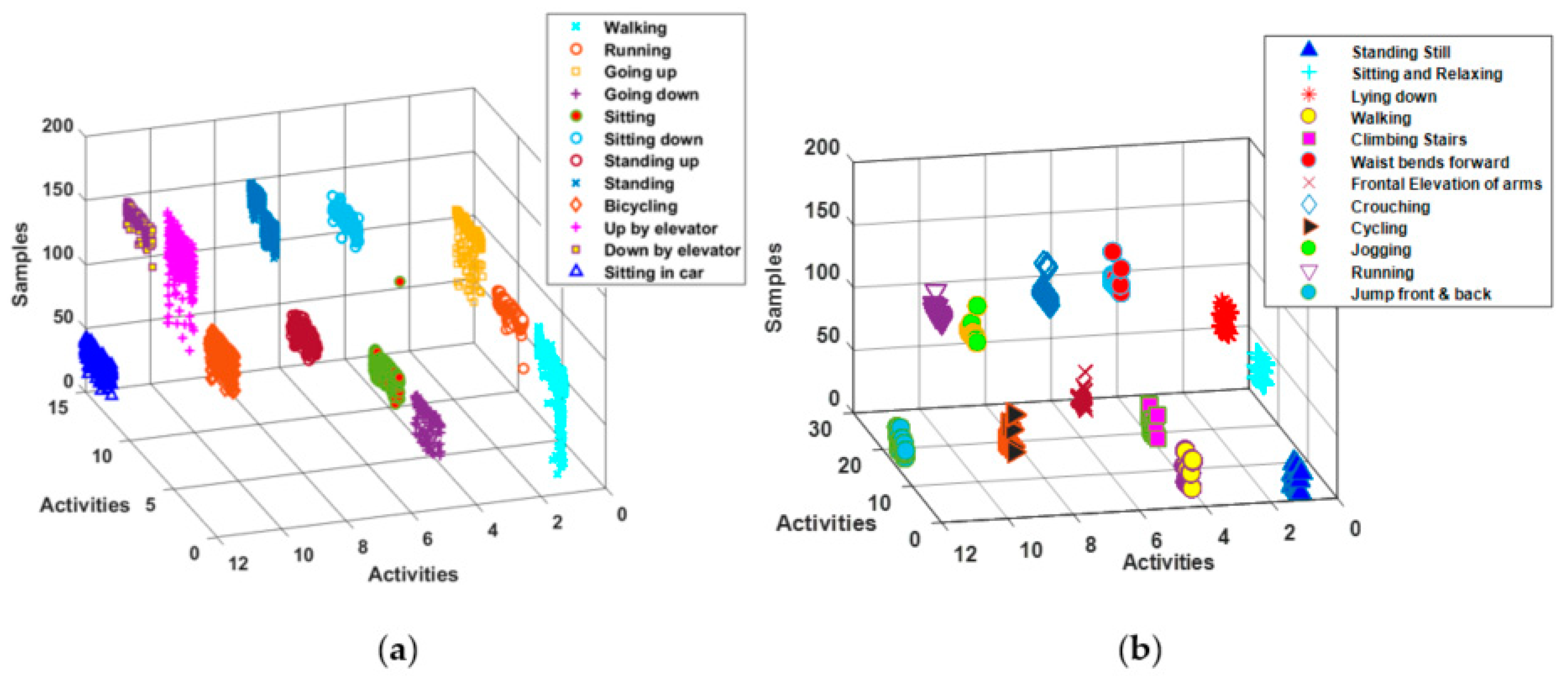
Figure 16.
Codebook generation via a GMM–GMR model applied to the (a) HuGaDB and (b) mHealth datasets.
Figure 16.
Codebook generation via a GMM–GMR model applied to the (a) HuGaDB and (b) mHealth datasets.

Figure 17.
Architecture of DBN using RBMs.

Figure 18.
Discriminative RBM structure: the visible layer consists of y labels and z inputs.

Figure 19.
Signal representing Chest acceleration for standing still, sitting and relaxing, and lying down (left column), and Chest acceleration for walking, running, and jogging (right column).
Figure 19.
Signal representing Chest acceleration for standing still, sitting and relaxing, and lying down (left column), and Chest acceleration for walking, running, and jogging (right column).


Table 1.
Confusion matrix for SPHR classification of all activities using the mHealth dataset.
| Activities | L1 | L2 | L3 | L4 | L5 | L6 | L7 | L8 | L9 | L10 | L11 | L12 |
|---|---|---|---|---|---|---|---|---|---|---|---|---|
| L1 | 9 | 0 | 0 | 1 | 0 | 0 | 0 | 0 | 1 | 0 | 0 | 0 |
| L2 | 1 | 10 | 0 | 0 | 0 | 0 | 0 | 0 | 0 | 0 | 0 | 0 |
| L3 | 0 | 0 | 9 | 0 | 0 | 1 | 0 | 0 | 0 | 0 | 0 | 0 |
| L4 | 0 | 0 | 0 | 9 | 0 | 0 | 0 | 0 | 1 | 1 | 0 | 0 |
| L5 | 0 | 0 | 0 | 0 | 10 | 0 | 1 | 0 | 0 | 0 | 0 | 1 |
| L6 | 0 | 0 | 0 | 0 | 0 | 9 | 0 | 0 | 0 | 0 | 0 | 0 |
| L7 | 1 | 0 | 1 | 0 | 0 | 0 | 10 | 0 | 1 | 0 | 0 | 0 |
| L8 | 0 | 0 | 0 | 0 | 1 | 0 | 0 | 9 | 0 | 0 | 0 | 0 |
| L9 | 0 | 1 | 0 | 0 | 0 | 0 | 0 | 1 | 9 | 0 | 0 | 0 |
| L10 | 0 | 0 | 1 | 1 | 0 | 1 | 0 | 0 | 0 | 10 | 0 | 1 |
| L11 | 0 | 0 | 0 | 0 | 0 | 0 | 1 | 0 | 0 | 0 | 9 | 0 |
| L12 | 0 | 0 | 0 | 0 | 0 | 0 | 0 | 1 | 1 | 0 | 0 | 9 |
| Mean Accuracy = 93.33% | ||||||||||||
L1 = Standing Still; L2 = Sitting and Relaxing; L3 = Lying down; L4 = Walking; L5 = Climbing Stairs; L6 = Waist bending forward; L7 = Frontal elevation of the arms; L8 = Knees bending (crouching); L9 = Cycling; L10 = Jogging; L11 = Running; and L12 = Jumping back and forth. In addition, the diagonal values represent the exact accuracy rate for each activity.
Table 2.
Confusion matrix for the SPHR classification of all of the activities using the HuGaDB dataset.
Table 2.
Confusion matrix for the SPHR classification of all of the activities using the HuGaDB dataset.
| Activities | H1 | H2 | H3 | H4 | H5 | H6 | H7 | H8 | H9 | H10 | H11 | H12 |
|---|---|---|---|---|---|---|---|---|---|---|---|---|
| H1 | 10 | 1 | 0 | 0 | 0 | 0 | 0 | 0 | 0 | 0 | 0 | 0 |
| H2 | 0 | 9 | 1 | 0 | 0 | 0 | 0 | 0 | 1 | 0 | 0 | 0 |
| H3 | 0 | 0 | 9 | 0 | 0 | 0 | 0 | 0 | 0 | 0 | 0 | 0 |
| H4 | 0 | 0 | 0 | 9 | 0 | 0 | 1 | 0 | 0 | 1 | 0 | 0 |
| H5 | 1 | 0 | 0 | 0 | 9 | 0 | 0 | 0 | 0 | 0 | 0 | 0 |
| H6 | 0 | 0 | 0 | 0 | 1 | 10 | 0 | 0 | 0 | 0 | 0 | 0 |
| H7 | 0 | 1 | 0 | 0 | 0 | 1 | 9 | 1 | 0 | 0 | 0 | 0 |
| H8 | 0 | 0 | 0 | 1 | 0 | 0 | 0 | 9 | 0 | 1 | 0 | 1 |
| H9 | 0 | 0 | 1 | 0 | 0 | 0 | 0 | 0 | 9 | 0 | 0 | 0 |
| H10 | 0 | 0 | 0 | 0 | 0 | 0 | 0 | 0 | 0 | 10 | 0 | 0 |
| H11 | 0 | 0 | 0 | 0 | 0 | 0 | 0 | 0 | 1 | 0 | 9 | 0 |
| H12 | 0 | 0 | 0 | 0 | 1 | 0 | 0 | 0 | 0 | 0 | 0 | 9 |
| Mean Accuracy = 92.50% | ||||||||||||
H1 = Waking; H2 = Running; H3 = Going up; H4 = Going down; H5 = Sitting; H6 = Sitting down; H7 = Standing up; H8 = Standing; H9 = Bicycling; H10 = Going up by elevator; H11 = Going down by elevator; and H12 = Sitting in a car. In addition, the diagonal values represent the exact accuracy rate for each activity.
Table 3.
Comparison of the sensitivity and specificity of the classification results using the mHealth dataset.
Table 3.
Comparison of the sensitivity and specificity of the classification results using the mHealth dataset.
| Activities | Sensitivity | Specificity |
|---|---|---|
| L1 | 0.692 | 0.984 |
| L2 | 0.758 | 0.992 |
| L3 | 0.687 | 0.992 |
| L4 | 0.692 | 0.984 |
| L5 | 0.763 | 0.984 |
| L6 | 0.687 | 0.992 |
| L7 | 0.775 | 0.975 |
| L8 | 0.687 | 0.992 |
| L9 | 0.703 | 0.983 |
| L10 | 0.775 | 0.967 |
| L11 | 0.677 | 0.992 |
| L12 | 0.698 | 0.984 |
Table 4.
Comparison of the sensitivity and specificity of the classification results using the HuGaDB dataset.
Table 4.
Comparison of the sensitivity and specificity of the classification results using the HuGaDB dataset.
| Activities | Sensitivity | Specificity |
|---|---|---|
| H1 | 0.800 | 0.991 |
| H2 | 0.732 | 0.983 |
| H3 | 0.720 | 1.000 |
| H4 | 0.726 | 0.983 |
| H5 | 0.726 | 0.991 |
| H6 | 0.800 | 0.991 |
| H7 | 0.732 | 0.974 |
| H8 | 0.732 | 0.974 |
| H9 | 0.726 | 0.991 |
| H10 | 0.800 | 1.000 |
| H11 | 0.714 | 0.992 |
| H12 | 0.720 | 0.991 |
Table 5.
Precision, Recall, and F-measure classification results using the mHealth and HuGaDB datasets.
Table 5.
Precision, Recall, and F-measure classification results using the mHealth and HuGaDB datasets.
| Activities | Precision | Recall | F-Measure |
|---|---|---|---|
| L1 | 0.818 | 0.818 | 0.818 |
| L2 | 0.909 | 0.909 | 0.909 |
| L3 | 0.818 | 0.900 | 0.857 |
| L4 | 0.818 | 0.818 | 0.818 |
| L5 | 0.909 | 0.833 | 0.870 |
| L6 | 0.818 | 1.000 | 0.900 |
| L7 | 0.833 | 0.769 | 0.800 |
| L8 | 0.818 | 0.900 | 0.857 |
| L9 | 0.692 | 0.818 | 0.750 |
| L10 | 0.909 | 0.714 | 0.800 |
| L11 | 1.000 | 0.900 | 0.947 |
| L12 | 0.818 | 0.818 | 0.818 |
| Mean | 0.847 | 0.850 | 0.845 |
| H1 | 0.909 | 0.909 | 0.909 |
| H2 | 0.818 | 0.818 | 0.818 |
| H3 | 0.818 | 1.000 | 0.900 |
| H4 | 0.900 | 0.818 | 0.857 |
| H5 | 0.818 | 0.900 | 0.857 |
| H6 | 0.909 | 0.909 | 0.909 |
| H7 | 0.900 | 0.750 | 0.818 |
| H8 | 0.900 | 0.750 | 0.818 |
| H9 | 0.818 | 0.900 | 0.857 |
| H10 | 0.833 | 1.000 | 0.909 |
| H11 | 1.000 | 0.900 | 0.947 |
| H12 | 0.900 | 0.900 | 0.900 |
| Mean | 0.877 | 0.880 | 0.875 |
Table 6.
Comparisons of the RBM layers in the deep belief network for the mHealth and HuGaDB datasets.
Table 6.
Comparisons of the RBM layers in the deep belief network for the mHealth and HuGaDB datasets.
| Dataset | No. of RBMs-Performance Method | No. of Epochs | No. of Nodes in Each RBM | Average Reconstruction Error | Time (s) |
|---|---|---|---|---|---|
| mHealth | r = 1 Reconstruction | 7 | n = 500 | 49,458,754.7895 | 2290 |
| r = 2 Reconstruction | 7 | n = 500 | 24,327.784 | 4689 | |
| r = 3 Reconstruction | 7 | n = 500 | 0.04582 | 6087 | |
| r = 4 Reconstruction | 7 | n = 1000 | 0.00037 | 8786 | |
| r = 5 Classification | 7 | n = 12 | 0.0000002 | 12,784 | |
| HuGaDB | r = 1 Reconstruction | 7 | n = 500 | 65,215,315,432.3545 | 2340 |
| r = 2 Reconstruction | 7 | n = 500 | 78,652,131.2563 | 4808 | |
| r = 3 Reconstruction | 7 | n = 500 | 156,325.012 | 7090 | |
| r = 4 Reconstruction | 7 | n = 1000 | 0.024563 | 10,910 | |
| r = 5 Classification | 7 | n = 12 | 0.000000284 | 15,580 |
Table 7.
Comparison of the proposed model with state-of-the-art deep learning algorithms using the mHealth and HuGaDB datasets.
Table 7.
Comparison of the proposed model with state-of-the-art deep learning algorithms using the mHealth and HuGaDB datasets.
| Method | Accuracy Using mHealth (%) | Method | Accuracy Using HuGaDB (%) |
|---|---|---|---|
| Abedin et al. [72] | 57.19 | Fang et al. [73] | 79.24 |
| Maitre et al. [74] | 84.89 | Rasnayaka et al. [75] | 85 |
| O’Halloran et al. [76] | 90.55 | Sun et al. [77] | 88 |
| Tahir et al. [23] | 90.91 | Badawi et al. [25] | 88 |
| Masum et al. [78] | 91.68 | Kumari et al. [79] | 91.1 |
| Ha et al. [80] | 91.94 | - | - |
| Guo et al. [81] | 92.3 | - | - |
| Proposed HF-SPHR Model | 93.33 | Proposed HF-SPHR Model | 92.50 |
Table 8.
Comparison of DBN, Random Forest, and AdaBoost Classifiers for the mHealth and HuGaDB datasets.
Table 8.
Comparison of DBN, Random Forest, and AdaBoost Classifiers for the mHealth and HuGaDB datasets.
| Algorithm | Dataset | Accuracy | Dataset | Accuracy |
|---|---|---|---|---|
| DBN | mHealth | 93.33% | HuGaDB | 92.50% |
| Random Forest | mHealth | 92.7% | HuGaDB | 91.9% |
| Adaboost | mHealth | 49.9% | HuGaDB | 57.0% |
Publisher’s Note: MDPI stays neutral with regard to jurisdictional claims in published maps and institutional affiliations. |
© 2021 by the authors. Licensee MDPI, Basel, Switzerland. This article is an open access article distributed under the terms and conditions of the Creative Commons Attribution (CC BY) license (http://creativecommons.org/licenses/by/4.0/).
Share and Cite
MDPI and ACS Style
Javeed, M.; Gochoo, M.; Jalal, A.; Kim, K. HF-SPHR: Hybrid Features for Sustainable Physical Healthcare Pattern Recognition Using Deep Belief Networks. Sustainability 2021, 13, 1699. https://0-doi-org.brum.beds.ac.uk/10.3390/su13041699
AMA Style
Javeed M, Gochoo M, Jalal A, Kim K. HF-SPHR: Hybrid Features for Sustainable Physical Healthcare Pattern Recognition Using Deep Belief Networks. Sustainability. 2021; 13(4):1699. https://0-doi-org.brum.beds.ac.uk/10.3390/su13041699
Chicago/Turabian StyleJaveed, Madiha, Munkhjargal Gochoo, Ahmad Jalal, and Kibum Kim. 2021. "HF-SPHR: Hybrid Features for Sustainable Physical Healthcare Pattern Recognition Using Deep Belief Networks" Sustainability 13, no. 4: 1699. https://0-doi-org.brum.beds.ac.uk/10.3390/su13041699
Note that from the first issue of 2016, this journal uses article numbers instead of page numbers. See further details here.