Feasibility and Economic Impacts of the Energy Transition


1
iMMC (Institute of Mechanics, Materials and Civil Engineering), Université Catholique de Louvain, 1348 Louvain-la-Neuve, Belgium
2
Université Lille, CNRS, IESEG School of Management, UMR 9221-LEM-Lille Économie Management and IRES, Université Catholique de Louvain, 1348 Louvain-la-Neuve, Belgium
*
Author to whom correspondence should be addressed.
Sustainability 2021, 13(10), 5345; https://0-doi-org.brum.beds.ac.uk/10.3390/su13105345
Submission received: 4 March 2021
/
Revised: 30 April 2021
/
Accepted: 4 May 2021
/
Published: 11 May 2021
Abstract
:There is currently no consensus regarding whether or not renewable energies are capable of supplying all of our energy needs in the near future. To shed new light on this controversy, this paper develops a methodology articulating a macroeconomic model with two sectors (energy and non-energy) and an energy model that is able to calculate the maximum potentials of solar and wind energy. The results show that, in a business-as-usual context, a complete energy transition on a global scale is unachievable before the end of the century. The reason lies in the increasing capital needs of the energy sector, which slows, if not stops, economic growth and the energy transition. A complete transition can be achieved by 2070 provided that (i) energy demand is kept under control at its current level, (ii) a sufficient rate of capital growth is sustained (above its historical level), and (iii) substantial progress is made in terms of energy efficiency. However, this strategy requires a significant increase in the savings rate, with a negative impact on consumption, which ends up stagnating at the end of the transition.
1. Introduction
In recent years, a controversy has developed as to whether, within a few decades, renewable energies could meet all of the world energy needs, without jeopardising economic growth. Many articles have been published in the literature, but there is clearly no consensus regarding the answer to this question. The dominant position answers positively [1,2,3,4,5,6,7,8]: an energy transition (ET) to a fully renewable energy system is possible within a few decades while ensuring economic growth (the interested reader will find further contributions to the dominant position in the extensive literature reviews made by Moriarty and Honnery [9] and Capellán-Pérez et al. [10]). Such a transition would be made possible by (i) increased energy efficiency, (ii) technical progress increasing the quality of the means of energy production (e.g., solar panels), and (iii) a reduction in the manufacturing costs of these means (in particular, by exploiting the economies of scale allowed by mass production).
There are distinctions within this dominant position. Some studies propose scenarios where the ET is accompanied by an increase in energy consumption [7]. The development of renewable resources should then not only replace fossil resources, but also allow for further energy growth. Other studies present scenarios, which, on the contrary, are based on the possibility of an absolute decoupling between the production of goods and services and energy consumption. In this context, economic growth would be accompanied by a decrease or stagnation of energy consumption [4,11]. This decrease would be made possible thanks to technical progress, but also to more sober behaviours in terms of energy use.
The position that is presented in the previous paragraphs is dominant, but not unanimous. Various recent contributions [9,10,12,13,14], which we shall refer to by the expression “critical literature”, have highlighted that the ET could result in an exacerbation of the capital needs of the energy sector, with a possible crowding out effect on the rest of the economy regarding the allocation of investment. This effect would negatively affect economic growth and, if strong enough, the ET could be accompanied by a prolonged phase of (imposed) economic decline.
Some of these contributions are based on models that highlight the close relationship between the energy sector and the rest of the economy (the dominant position is also based on models, particularly of the IAM type. For a critique of the latter, see [10]). It is interesting to note that they are based on different, sometimes even opposing, methodologies and assumptions. Some models, such as GEMBA [15,16] and MEDEAS [10], belong to systems theory. Others belong to the economic theory of growth [17,18]. Unlike the former, they assume market equilibrium and explicitly model the behaviour of economic agents. Only the EENGM model of Režný and Bureš [19] was found to combine the two methodologies. This article also provides an interesting review of a set of energy-economic models. For another review of this type of models, see Rye and Jackson [20].
In all of these contributions, the crowding out effect mentioned above is associated with a decrease in energy efficiency (known as the acronym Energy Return On Investment (EROI)), that affects both non-renewable and renewable energy technologies. On the one hand, the EROI of fossil resources would decrease as they become increasingly difficult to extract. On the other hand, the EROI of renewable energy technologies appears to be (significantly) lower than the historical levels that are achieved by the EROI of fossil-based energy production. On top of that, despite technical progress, the EROI of renewables could decrease in the future due to a location effect linked to the lower "quality” of remaining available sites for additional installations to harvest these resources.
This location effect is particularly well highlighted by Dupont et al. [21,22] at the global level for wind and solar energy. As stated by Moriarty and Honnery [9], these two sources will play the main role in the upcoming ET.
The aim of this paper is to couple the macroeconomic model that was developed by Fagnart and Germain [23] and Dupont et al. [24], accounting for the crowding out effect, with the energy models of Dupont et al. [21,22], accounting for the location effect. The macroeconomic model, an input–output type model with two sectors (energy and non-energy), has the advantage of being relatively high-level (as compared to other much more detailed models) and to lead to transparent analytical results linking economic growth to the penetration rate of renewable energies. The energy models are able to calculate the maximum potentials of solar and wind energy on a global scale, from a very detailed description of the local potentials.
The articulation of the previous models allows us to answer the following questions: given a future trajectory of the energy demand, hypotheses on the evolution of the technical parameters of the economy and on the behaviour of economic agents in terms of consumption and savings, (i) is a complete ET possible and (ii), if so, at what pace? As a corollary, it is possible to determine the conditions that ensure that the ET is completed over a given period of time.
The structure of the article is as follows. Section 2.1 presents the macroeconomic model and EROI formula, Section 2.2 the energy model, and Section 2.3 and Section 2.4 the articulation between these two models. Section 2.5 presents the calibration of the macroeconomic model for a reference year, based on [24], and Section 2.6 formulates the hypotheses regarding the future evolution of some exogenous parameters. Section 3 presents the results of the various simulations of the ET, based on assumptions regarding (i) the behaviour of economic agents in terms of consumption and savings and (ii) the potential and pace of technical progress achievable in the coming decades. The end of the section discusses the main assumptions and their impacts on the simulation results.
2. Materials and Methods
2.1. The Macroeconomic Model
The macroeconomic model (MM) was extensively presented in a previous publication [24]. In the following subsections we recall its main characteristics for the understanding of the following work.
2.1.1. Main Features
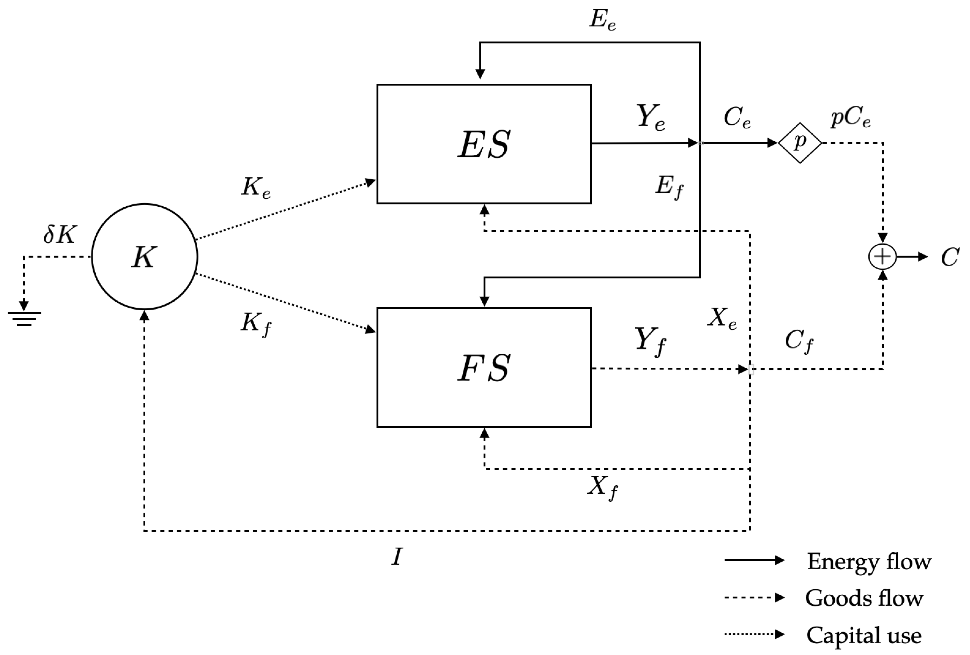
The model (as illustrated in Figure 1) is that of a closed economy, with two sectors: (i) the energy sector (ES), which produces energy for the rest of the economy, and (ii) the non-energy sector (FS), which produces a general-purpose good used for intermediate and final consumptions and for investment. The output of the ES is distributed between energy intermediate consumptions (EIC) of the two sectors and deliveries for final consumption, final referring to private (household) as well as public (government) consumption. Both of the sectors use three factors of production: capital, energy, and goods (in the following, we will refer to the intermediate consumption of goods that are produced by the non-energy sector as non-energy intermediate consumption (NEIC)). The capital stock of the economy is shared between the two sectors according to their respective needs.
2.1.2. Mathematical Formulation
The energy and non-energy sectors are identified by the indices e and f, respectively. The model is dynamic in the sense that the variables are discrete functions of time. However, time-dependency is omitted in the equations to simplify the notations.
The sectoral outputs and factor consumptions are linked by the following relationships:
where:
- , , , and refer to the production, capital stock, EIC, and NEIC of sector i, respectively. Energy production and consumption are measured in units of energy (); good production, NEIC, and capital stock in units of good produced by the FS ().
- , , and refer to the capital, EIC, and NEIC intensities of sector i, respectively, i.e., the quantities of these inputs per unit of output. These intensities are likely to change over time as technologies evolve.
The total capital stock is shared between the two sectors:
Capital accumulation is described by:
where I and refer to the gross and net investments, respectively. refers to the average depreciation rate of capital (). It is the weighted average of the sectoral depreciation rates:
Further, the growth rate of a given variable x is defined as . In particular, the capital growth rate is defined as:
The production of the FS is divided into sectoral NEIC, deliveries for final consumption, and investment:
The output of the ES is divided between sectoral EIC and final energy consumption (that is defined as private and public consumption of energy, similarly to the final consumption of goods):
The total consumption is defined as the sum of final consumptions (of goods and energy):
The price of the production good is chosen as the numeraire and is equal to 1. With p being the real price of energy (in ), the sectoral gross added values (AV) are calculated as:
By definition, the gross domestic product (GDP) is the sum of the sectoral added values, i.e.:
The second equality derives from Equations (9) and (10) and it splits the GDP in terms of sectoral deliveries to the final demand. From Equations (6)–(11), one can easily rewrite Equation (11) to express the GDP as the sum of total consumption and investment:
The sectoral net added values (NV) are obtained from the gross sectoral added values by subtracting the sectoral consumptions of capital (understood as the depreciation of capital in the two sectors):
The technical parameters represent the consumption of goods of the two sectors per unit produced, in the form of NEIC and capital consumption.
By definition, the net domestic product (NDP) is the sum of the sectoral net added values. Given the previous equations, one obtains:
From Equations (3) and (12), one also obtains:
NDP accounts for the useful output of the economy, which is used for total consumption and economic growth.
The macroeconomic savings rate is defined by:
It represents the share of GDP invested in capital production, with the remaining going to final consumption. It follows that:
The share of energy in total consumption is defined by:
Parameters s and concisely describe savings and consumption choices.
A variable of interest for energy-economy models is the EROI and, in this paper, we will look at the point-of-use EROI. At the societal level, it corresponds to the ratio between the production of the ES that leaves the ES (i.e., the energy delivered, ) and all of its inputs expressed as energy flows (EIC , NEIC and capital ). In Appendix A, it is shown that the point-of-use EROI at the societal level can be calculated, as follows:
and being the energy content of the goods flows and .
2.2. The Energy Model
The energy model (EM) decomposes the ES into two subsectors: the renewable and non-renewable energy subsectors. The renewable energy subsector is based on the methodology that was developed by Dupont et al. [21,22]. It relies on the postulate, as advocated by Moriarty and Honnery [9], that wind and solar energy will represent the two main sources of energy in a 100% renewable world. This is a position shared by the International Energy Agence (IEA) and the U.S. Energy Information Administration (EIA) [25,26]. Indeed, although biomass is currently the leading source of renewable energy worldwide, it mainly concerns domestic use by the most deprived populations. Its intensive development for energy use is a source of serious controversy due to the potential competition with other essential uses (mainly food supply, but also biodiversity conservation, CO capture, etc.). Regarding other renewable energy sources, either their potential for future development is limited (hydropower), or their technical potential is relatively low (wave and tidal energies), or their development does not seem as promising as expected (geothermal energy). These considerations are shared by [4], since, in their projection for 2050, biomass is absent, hydropower represents 4% of the total production, and the sum of geothermal, tidal, and wave energies represents just over 1% of the total.
The aim of the EM is to quantify the potential of these two energies at a global level.
A spatial discretisation of the world is at the root of the EM. The spatial resolution is 0.75° × 0.75° (4000 km on average), which corresponds to a total of 114,000 terrestrial sites. For each terrestrial site, the area that is available for the implementation of wind or solar power plants is estimated by combining different databases, including, among others, the type of land use and the local slope of the land (which is a limiting factor for solar power plants), or the water depth and distance from the coast (for offshore wind). Based on the local resources (wind speed distribution and solar irradiation), the theoretical annual production of each technology considered is then calculated for each site.
The technologies considered are the following. Regarding wind energy, onshore and offshore wind up to 1000 m depth are taken into account. Among solar technologies, the ones taken into account are: (i) photovoltaic centralised power plants and residential installations (on rooftops), with 2 types of panels of different efficiencies and technologies, and (ii) 3 types of concentrated solar power plants (parabolic power plants with or without thermal storage, and solar towers with thermal storage). The wind and solar thermal technologies are optimised to be best adapted to the local site conditions. Wind turbines are optimised in terms of (i) their design to be best adapted to local climatic conditions and (ii) their spacing to reduce losses due to the wake effect (i.e., the interactions between successive rows of wind turbines). The design of thermal power plants (i.e., the size of the heliostat field in relation to the nominal power of the installation) is optimised to be best adapted to local sunlight conditions.
At each site, solar technologies (photovoltaic and thermal) compete for land use and the model selects the one with the best EROI. However, this is not the case between wind and solar power plants, as a given area can be occupied simultaneously by both types of installations.
Once the technological choices have been made at the level of each site, the EM calculates, per site and for each of the technologies used on the site, (i) the production potential, (ii) the direct and indirect energy inputs that are required per unit of energy produced and, by relating the two previous quantities, and (iii) the site EROI. On this basis, by ranking all combinations of sites and technologies in descending order of EROI, the EM provides the direct and indirect energy inputs and required producing a given aggregated amount of renewable energy (it is shown in Appendix B that the EROI ranking criterion leads to the same results as a ranking by profitability).
Thus, the EM provides two curves and over the interval , where designates the maximum production potential of wind and solar energy (potential being calculated by the EM, expressed in units of energy per year). These curves correspond to a discrete set of points, with each value corresponding to the potential of a given technology in a given geographical location. These two curves are used by the MM to calculate the technical parameters of the ES.
2.3. Articulation between the Two Models
The energy flows and are the energy contents (in units of energy ) of and , which refer, respectively, to the NEIC and capital consumption of the renewable energy subsector (in units of goods produced by the FS ). These quantities are related by:
where is the energy intensity (i.e., the energy content) of a unit of good that is produced by the FS.
It is then possible to calculate the technical coefficients of the renewable energy subsector, depending on its production:
Two assumptions are taken regarding the direct energy inputs . First, internal energy inputs are not accounted for in the MM (see [24]). As wind and solar facilities only consume operationnal electricity that is directly produced by the installation, the direct energy input related to the production of renewable electricity is assumed to be zero. However, should account for the losses in electricty that are associated with transport and distribution. According to the IEA statistics (https://www.iea.org/data-and-statistics, last acces on 10 May 2021) and MEDEAS [27], they represent about 9.5% of the electricity thta is consumed worldwide, i.e., 8.7% of the electricity produced. It gives that . The increase in distribution losses with renewable penetration (as described in the MEDEAS documentation) is not taken into account in the model, i.e., remains constant during the energy transition.
The intensities and as a function of are shown in Figure 2. The increasing rate of these intensities highlights the location effect mentioned in the introduction. Because of the lower “quality” of the sites that can receive the additional installations exploiting wind and solar resources, increasing capital and NEIC are needed to produce one unit of energy.
The renewable energy penetration rate is defined by the ratio . If is given, then the total renewable () and non-renewable () energy productions can be deduced. The technical parameters , , can also be expressed as functions of .
The parameters of the non-renewable energy subsector are determined by the following ratios:
If they are known, then the technical parameters of the ES are then determined as an average, weighted by , of the technical parameters of the two subsectors:
2.4. Allowable Space and Transition Curve
2.4.1. Allowable Space
The concept of allowable space (AS) emerges from the attempt to determine an exhaustive set of trajectories satisfying a given criterion. In the present case, the retained criterion is simply that the net sectoral added values are both positive:
This criterion reflects the fact that both sectors should contribute positively to the useful output of the economy (as measured by the NDP).
From Equations (13) and (14), we know that NV decreases and NV increases with p. Beyond , the price of energy is so high that NV is negative. Below , the price of energy is so low that NV is negative.
Under assumptions regarding the economic choices in terms of consumption and investment, can be transformed into an interval for k, the capital/energy production ratio of the economy (Appendix D):
where is a vector of behavioural parameters, which contains either s and or s and , where refers to the capital growth rate. As was the case for the interval bounds for p, beyond , NV becomes negative (p is too high) and below , NV becomes negative (p is too low).
Among the technical parameters on which depends, , , and are functions of according to Equations (21)–(23), while the others do not vary with . Therefore, we can write Equation (27) as:
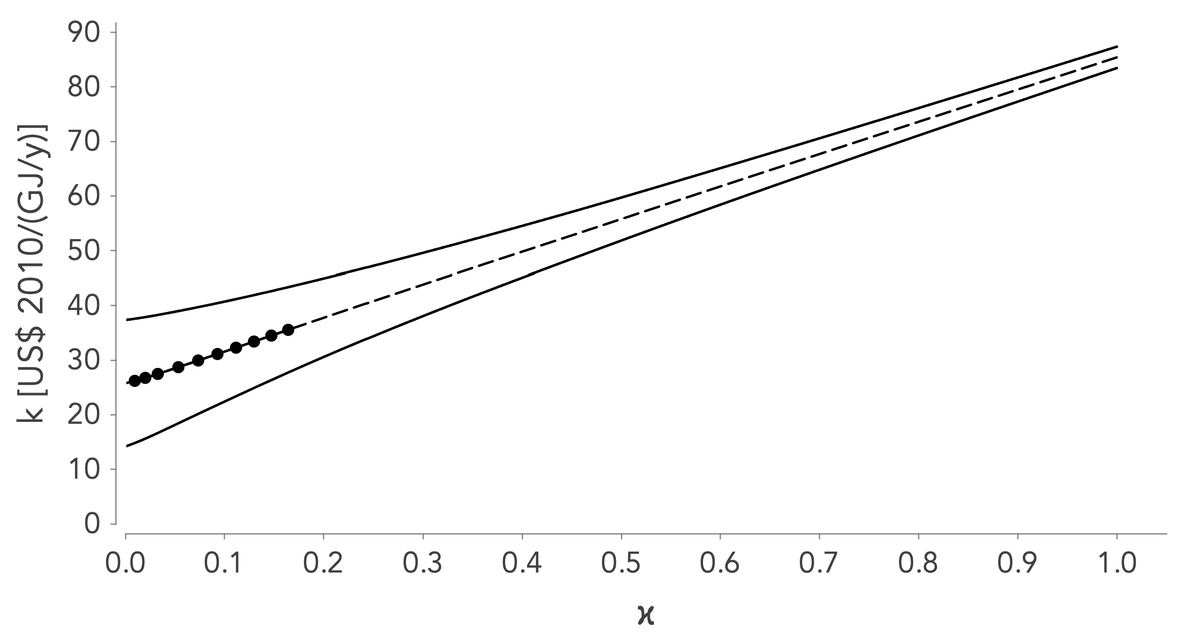
and are the top and bottom envelopes of the allowable space (AS), defined as all the couples that satisfy the criterion from Equation (24). The envelopes and are both increasing functions of , partly because renewable energies are more NEIC and capital intensive than non-renewable energies. The equations determining these envelopes are specified in Appendices Appendix D.2 and Appendix D.4, depending on the assumed economic choices in terms of consumption and investment.
An example of AS is illustrated by the space between the lower () and upper () curves shown in Figure 3.
2.4.2. Transition Curve
A tansition curve (TC) is a function such that:
derivable, increasing and contained in the AS. Consequently, a TC respects the following inequalities:
An example of TC is shown by the dotted curve presented in Figure 3. It is entirely located between the two envelopes and, therefore, respects the previous inequalities.
2.4.3. The Reduced Dynamic Model
The reduced dynamic model (RDM) is obtained from the MM, while integrating the notion of TC. It makes it possible to fully characterize the trajectory of an economy during its ET and, more precisely, to numerically determine whether (i) the ET is feasible or not in a finite time and (ii) if it is feasible, the time that is needed to complete it. Thanks to the MM, it is then possible to see the impact of the ET on all economic variables.
Two versions of the RDM are considered, which correspond to Exercises 1 and 2 described below, and that depend on different assumptions in terms of consumption and investment:
- Exercise 1: s and fixed.
- Exercise 2: and fixed.
Exercise 1 assumes a constant savings rate and a constant share of energy expenditure in total consumption. In this case, the capital growth rate is endogenous. Exercise 2, instead, assumes that the economy has a given capital growth rate to achieve at constant , and it results in an endogeneous savings rate. Exercises 1 and 2 are based on the common assumption that is constant. As part of this work, in order to test the sensitivity of the results to this hypothesis, a third exercise was analysed where s is constant and final good and energy consumption are assumed to be strictly complementary (in other words, the ratio is constant). When compared to Exercise 1, in that case the substitution between final good and energy is less easy at the level of consumption choices. Exercise 1 and this third exercise are in fact polar cases in the sense that, for a given budget, they are respectively based on the assumption that the agents maximise either a Cobb-Douglas or a Leontief utility function (whose elasticities of substitution are, respectively, unitary and zero).
The results from Exercise 3 were most of the time favourable to the ET. For some TCs and in the framework of the sustainable development scenario, it can even be completed in a few decades. However, these results are questionable, as they imply a sharp rise of the price of energy during the ET, making the constant hypothesis unlikely.
Exercise 1—s and η Fixed
Within the context of Exercise 1, it is possible, thanks to the MM, to express as a function of k, , s and the other parameters (Appendix D.3):
where
The first term of the right-hand side member of Equation (30) is an increasing function of k, , and s (because ), and a decreasing one of As the second term, , is also an increasing function of k and a decreasing one of , follows the same trends. It follows that, if is positive, K also increases, and, thus, for a given , k also increases. Ceteris paribus, there exists a positive feedback loop between and k. However, this loop does not result in explosive growth, since, if tends to ∞, tends to a positive constant. On the other hand, is negatively affected by the ET. As increases, so do and , resulting in a lower share of the FS output being available for its own investment. This exacerbation of the needs of the ES (mainly in terms of capital) to the detriment of the FS, mathematically translated by the fact that , is the manifestation of the crowding out effect mentioned in the introduction.
Exercise 2— and fixed
Within the context of Exercise 2, it is possible, thanks to the MM, to express s as a function of k, , , and the other parameters (Appendix D.5):
where is defined by Equation (31). s is a decreasing function of k and an increasing function of and , provided that is not too much higher than . For a constant , an economy with more capital produces more goods, which allows a lower relative savings rate to achieve the investment needed to sustain the desired growth rate . On the contrary, a higher renewable penetration rate diverts capital away from the FS, which results in less goods being produced and the need of more relative savings to reach .
The RDM for Exercise 1 consists of Equations (28)–(30), (21)–(23), and the identity defining (Equation (5)). The RDM for Exercise 2 consists of the same equations, except that Equation (32) replaces Equation (30).
Although the time dependency has not been explicited in the formulas, the RDM is a (discrete) dynamic model. The solution procedure of the RDM works, as follows. Given the evolutions over time of the energy demand , of the technological parameters (in particular, ), and of the TC, the RDM is used to determine the trajectory of and during the ET and the time that is needed to complete it (i.e., to reach ). Knowing the capital stock , the capital growth rate is either calculated via Equation (30) (Exercise 1) or imposed (Exercise 2), and the capital stock is calculated via (5). is exogenously determined and can be deduced via Equation (26). The penetration rate of renewable energy is then determined by inverting Equation (29). Finally, thanks to Equations (21)–(23), the values of the ES parameters (, , and ) are calculated. Once the previous variables have been determined, all of the other economic variables (sectoral production, consumption, GDP, etc.) can be calculated via the MM.
The first time periods of an example of ET in the AS are illustrated by the black dots shown in Figure 3, in the particular case where all exogenous technical parameters are constant (the envelopes of the AS and the CT are, therefore, not time-dependent). It is important to clearly distinguish the TC (dotted curve) from the trajectory representing the ET (the points). Mathematically, the TC is continuous while the trajectory is a discrete set. If the TC is postulated and, therefore, exogenous, the pace of the ET along the curve is endogenous and it is this pace that determines the ET actually observed.
Finally, it should be noted that there are two contradictory forces influencing the ET. On the one hand, the positive loop between k and noted above favours the growth of k and, thus, the ET. On the other hand, the ET results in an increase of and , which have a negative effect on growth. If an increase of k was to be accompanied by a too strong increase in these parameters, then could become negative, leading to further decreases of k and , which would block the transition. Therefore, for the ET to have a chance to continue, it must be done with enough available capital.
2.5. Calibration of the Macroeconomic Model
In [24], the variables of the MM are calibrated on the basis of global observations or estimates for a so-called reference year. A sensitivity analysis shows that the calibration is not very sensitive to variations in these parameters.
Subsequently, the units of good () and energy () of the theoretical model are translated into real units: respectively, 2010 US dollars (US$ 2010) and Joules (J).
Observed data
These are (i) IEA data for final energy consumption (https://www.iea.org/data-and-statistics, last access on 10 May 2021), and (ii) World Bank statistics for economic data: GDP and savings rate (https://data.worldbank.org: Gross savings (% of GDP) (s) and Gross added value at basic prices (GVA) (constant 2010 US$)) (GDP), last access on 10 May 2021).
Estimated data
Five model parameters have to be estimated in order to allow for the calibration of the whole model. These parameters are:
- Sectoral capital depreciation rates. Based on the literature, the lifetime of capital in the ES is estimated at 25 years, and that in the FS at 20 years. This gives and .
- The share of total capital devoted to the ES, as measured by the ratio . The calibration of the GEMBA model [16] provides the value μ =6.5%.
- The share of energy expenditure in the total household and state budget measured by (Equation (19)). On the basis of the OECD input-output tables, an estimate of 4% is found for 2015.
Calibrated data
The observed and estimated data allow for the calibration of the model parameters and variables, for the chosen reference year (2018). The technical parameters of the two sectors and the EROI are listed in Table 1.
Knowing the technical parameters of the ES in 2018 (Table 1), the corresponding renewable penetration rate (according to the IEA statistics, wind and solar accounted for 2% of the total primary energy supply in 2018, i.e., ), and the evolution of the technical parameters of the renewable subsector thanks to the EM, the technical parameters of the non-renewable subsector (i.e., , , ) are found via Equations (21)–(23), see Table 2).
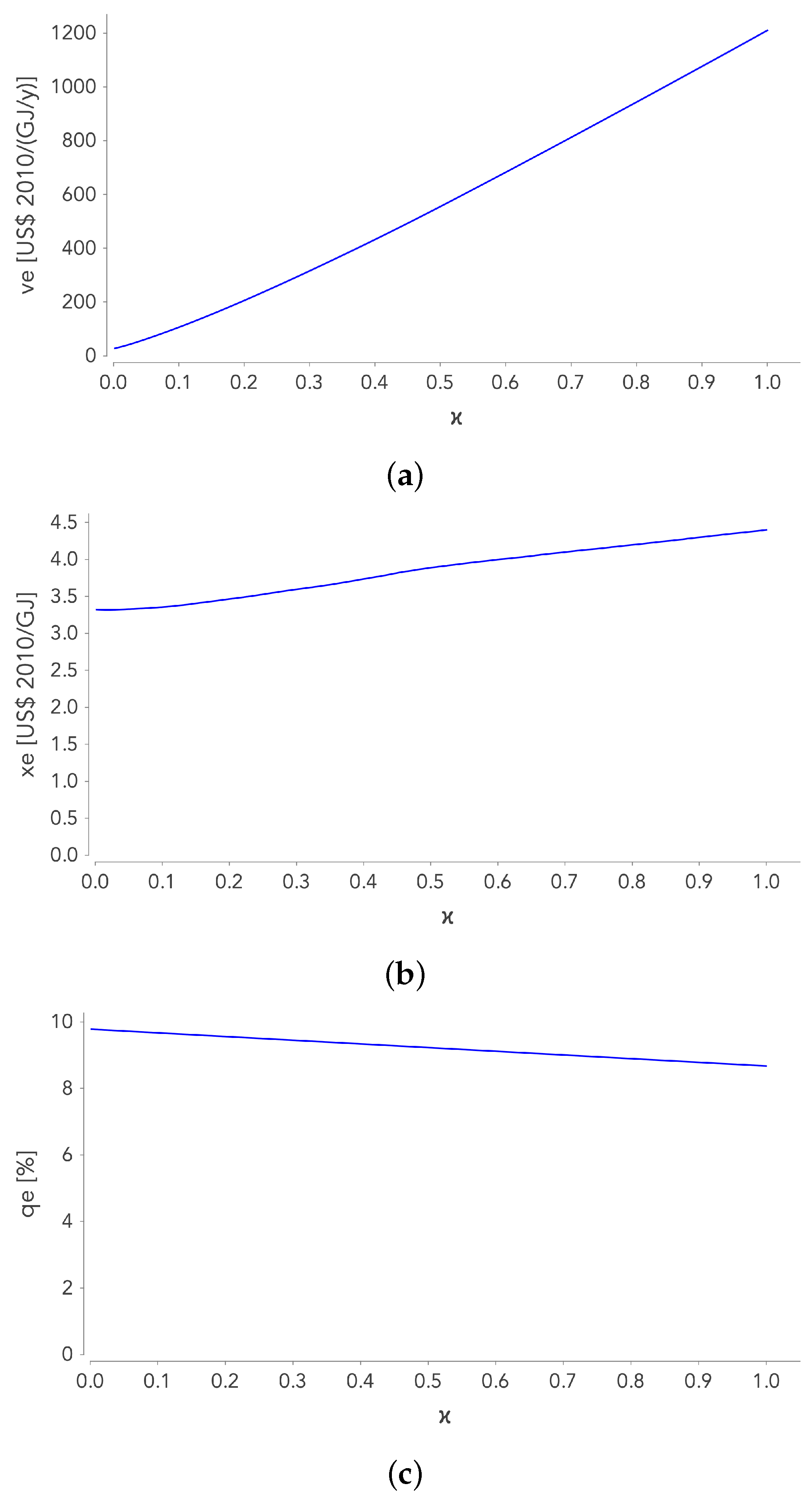
Figure 4 presents the evolution of the technical parameters of the ES as a function of the penetration rate , in the particular case where is also set at its 2018 value (thus, for , ). evolves between 0 (all energy production is provided by non-renewable energies) and 1 (all of the energy production is provided by wind and solar technologies).
- Figure 4a shows that the capital intensity increases considerably with the penetration rate : , which is consistent with the common assumption that renewable energies are much more capital intensive than non-renewable energies.
- Figure 4b shows that increases slightly with the ET: . The NEIC requirements are not much higher for renewable energies than for non-renewable energies.
- Because and , the energy intensity slightly decreases with (Figure 4c).
Historical values of s and
Within the framework of the simulations, either the value of the savings rate s or the capital growth rate will be set at its historical level. To do this, the value averaged over the last five years was used. We find, for the period 2014–2018, for s, an average value of 25.05% and, for , an average value of 2.27%.
2.6. Future Evolution of the Parameters
Future changes in the technical parameters of the two sectors and energy demand are based on the following assumptions:
- The evolution of the technical parameters of the ES with the ET is described by Equations (21)–(23), where the technical parameters of the non-renewable energy subsector are assumed to be constant and equal to their calibrated value in 2018 (see Table 2). Assuming that the parameters of the non-renewable energy subsector will not change in the future can be considered to be optimistic. Given the maturity of the technologies, technological progress seems to be limited and not able to counterbalance the depletion of the resources. It is therefore likely that in the future there will be an increase in the energy and capital intensities of the non-renewable energy subsector.
- Based on past values, the parameters and are assumed to be constant. Indeed, the MM calibration performed over the last 30 years shows that these parameters have not changed since 1990 (see Appendix E).
- The changes in and are based on the IEA’s "World Energy Outlook” 2020 report [25]. There are two scenarios: (i) the business-as-usual scenario (BAU), where changes in and are extrapolated on the basis of the last 30 years (by 2040, increases by 45% and decreases by 15%) and (ii) the sustainable development scenario (SD), which assumes a constant energy demand and a rapidly decreasing energy intensity in the coming decades (by 2040, would decrease by 40%, which corresponds to a rate of decline never observed in the past) (see Appendix F for further details). In the long term, both of the scenarios have the same technical progress potential in the FS ( is asymptotically reduced by 50%), the difference between the two scenarios being the pace at which this limit is reached. A third scenario based on the IEA’s New Policies scenario was also tested, but did not lead to fundamentally different results from those of the BAU scenario.
3. Results
Thereafter, we consider TCs in the form of weighted averages of the AS envelopes, i.e., curves of the form:
where (i) is the weighting parameter and (ii) and are the envelopes of the AS defined by Equations (A9) (Exercise 1) and (A13) (Exercise 2). As the energy intensity of the FS decreases over time (see Section 2.6), the envelopes of the AS and the TC are both functions of t. is exogenous, constant, or a function of t, chosen so as to always respect inequalities . The formulation from Equation (33) then ensures that the TC remains within the AS in each time period.
3.1. Exercise 1—s and η Given
3.1.1. Impact of
The purpose of this subsection is to scan the entire AS and measure how the results change when the TC move through this space. A simple way to do this is to consider all of the TCs with a constant weighting parameter .
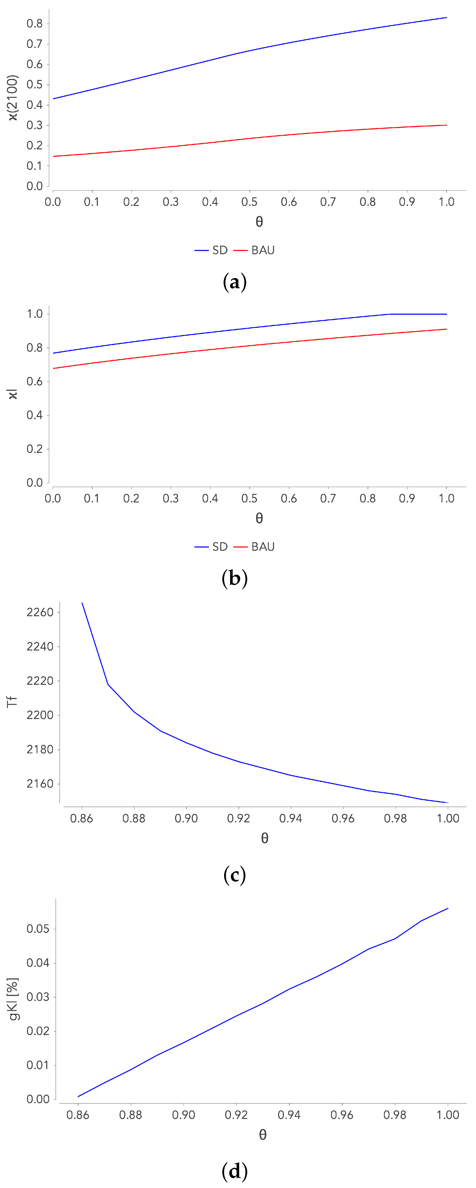
The graphs shown in Figure 5 provide, for the two scenarios: (i) , the renewable penetration rate in 2100, (ii) , the asymptotical value of , (iii) if it is completed in a finite time, the year of the end of the ET, , and (iv) if any, the residual capital growth rate at the end of the transition, . When the transition is completed in a finite time = 1, if not, is obtained when no longer varies, because tends towards 0. There is a residual capital growth rate when the transition is completed in a finite time. However, this residue is very low and never exceeds 0.06%.
Business-as-usual scenario (red curves)
- Figure 5a gives the value of the penetration rate in 2100. The curve is slightly increasing, but is approaching 30% at best.
- Figure 5b shows that the ET is never completed in a finite time. Nevertheless, we see that is approaching 1 for , and is above 65% for all values of . The non-completion of the ET is due to the fact that the growth rate of the capitak stock decreases down to zero.
- As mentioned above, the residual growth rate of the capitak stock is 0 for all the simulations. The economy tends towards a stationary state with no growth.
Sustainable development scenario (blue curves)
- Figure 5a shows that the renewable penetration rate in 2100 is significantly higher for SD than for BAU.
- Figure 5b shows that, if no scenario allows for a complete ET in a finite time.
- Figure 5c shows that for the duration of the ET decreases with (from 248 years for to 131 years for ). The minimum value of is reached for (a complete transition by 2149).
- Figure 5d shows that the residual capital growth rate is 0 for and sightly increasing for . At best, it reaches 0.056%.
The previous results only concern TCs with a constant weighting rate. However, numerically, the following conjecture is verified:
Consider a TC defined by (33), whose weighting parameter is variable and described by the sequence Let () be the maximum of this sequence. Let be the TC whose weighting parameter is constant and equal to . Subsequently,
The interest of this result is to provide a minimum bound for the duration of an ET based on a TC with variable weighting parameter, from the values of calculated for TCs with constant weighting parameter (the values given by Figure 5c).
As a corollary of this conjecture, the duration of any ET will be greater than or equal to , where designates the TC characterised by (i.e., greater than 104 years for SD). As a reminder, simulations with would correspond to an economy where the net added value of the FS is zero. The price of energy is so high that all of the added value of the economy comes from the ES.
3.1.2. Impact of the Technical Progress Rate
Whether for BAU or SD, the technical progress potential is assumed to be very high, since the energy intensity of the FS is asymptotically divided by 2. The difference between the two scenarios lies in the potential already realised in 2040 (30% for BAU, 80% for SD).
Further increasing the potential realised in 2040 under SD does not fundamentally change the results of the previous subsection. For the record, the evolution of is governed by Equation (A15). If the rate of change is increased sharply to the point that the potential of technical progress is realised in a few years, the end of the ET (as measured by ) is slightly advanced, but remains beyond 2100.
Consequently, it appears from the previous simulations that, unless assuming unreasonable progress in terms of energy efficiency, it is not possible to achieve a complete ET before the end of the century, even when assuming energy demand control (as required by the SD scenario).
3.2. Exercise 2— and Fixed
Previous simulations have shown how difficult it would be to achieve a complete ET before the end of the century if consumption and savings choices remain unchanged. The aim of this section is to study an alternative strategy, aiming at supporting capital growth through an increase in the savings rate.
3.2.1. Impact of
As in Section 3.1.1, the following simulations are based on a constant weighting parameter . Table 3 shows the values of , s, and (in 2050, 2100, and ) obtained for Exercise 2 for and . The changes in the variables between these extreme values are monotonous. The capital growth rate is fixed at its average value over the last five years: 2.27%.
Business-as-usual scenario
The table shows that:
- The ET is completed in a finite time for and and, thus, for all values of . is slightly increasing with , but it varies little ( goes from 2129 for to 2133 for ). In Exercise 1, an increase of stimulated capital growth and, thereby, accelerated the ET. In Exercise 2, this effect is not present, since is fixed.
- The ET is far from being completed by the end of the century. varies between 46% for and 17% for .
- As for , the observed values of s at the end of the ET evolve little with (from 44% for = 0 to 41% for = 1).
In summary, this analysis reveals that all of the TCs included in the AS lead to a complete ET in about 115 years, with a significant increase in the savings rate.
Sustainable development scenario
Previous results have shown that, under the BAU scenario, maintaining the capital growth rate at its historical level through a gradual increase in the savings rate would allow a complete ET in about 115 years. The end of the transition does not occur until the next century.
However, in the context of Exercise 1, we have seen that the SD scenario made it possible to significantly reduce the duration of the ET when compared to BAU (see Section 3.1.1). Intuition then suggests that the combination of the hypotheses of Exercise 2 and the SD scenario should enable a complete ET before the end of the century.
In order to verify this, the previous analysis made for BAU is repeated for SD. Table 3 shows the values obtained. We observe that:
- The previous intuition is confirmed, since the completion of the ET is obtained after a period of 67 to 72 years, i.e., a value of around 2090.
- Maintaining the capital growth rate during the ET requires a significant increase in the savings rate s. However, this increase is less than for BAU, as s reaches between 37 and 40% at the end of the ET, depending on the value of .
From the above, it appears that the SD scenario, combined with the support of capital growth, allows for completing the ET before 2100.
3.2.2. SD: Required for
With the previous simulations, in the best case scenario, we are still beyond certain target dates retained in the literature in the fight against climate change. Indeed, according to a recent IPCC report [32], limiting the global temperature increase to 2 °C requires the achievement of carbon neutrality by 2070 (and a reduction of 25% in emissions by 2030 as compared to their 2010 level). The latter key date (2070) is also chosen by the IEA to achieve global carbon neutrality as part of the sustainable development scenario [33].
The previous point showed that maintaining the capital growth rate at its historical level (i.e., 2.27%, its average value over the last five years period) within the framework of SD made it possible to complete the ET in about seventy years. Intuition suggests that increasing the capital growth rate should lead to an even shorter transition.
The following simulation results are based on the objective of an end of the ET in 2070, and they aim at determining the growth rate necessary to reach this goal, as a function of . Table 4 shows that:
- increases slightly with , from 2.91% to 3.12%.
- The savings rate that was observed at the end of the ET decreases slightly with , while still remaining above 40%.Note: similar simulations can be carried out within the framework of BAU. To complete the transition by 2070, a capital growth rate of around 4.1% is required, depending on . To maintain this growth rate, a savings rate of more than 55% is then necessary (s at the end of the ET decreases from 58.6% for to 56.2% for ).
3.2.3. Temporal Analysis
Previous results show that an ET completed before the end of the century requires a significant increase in the savings rate, highlighting that the transition has a profound effect on the economy. Using the MM, the following analysis aims to shed light on the behaviour of economic variables during the transition of the ES.
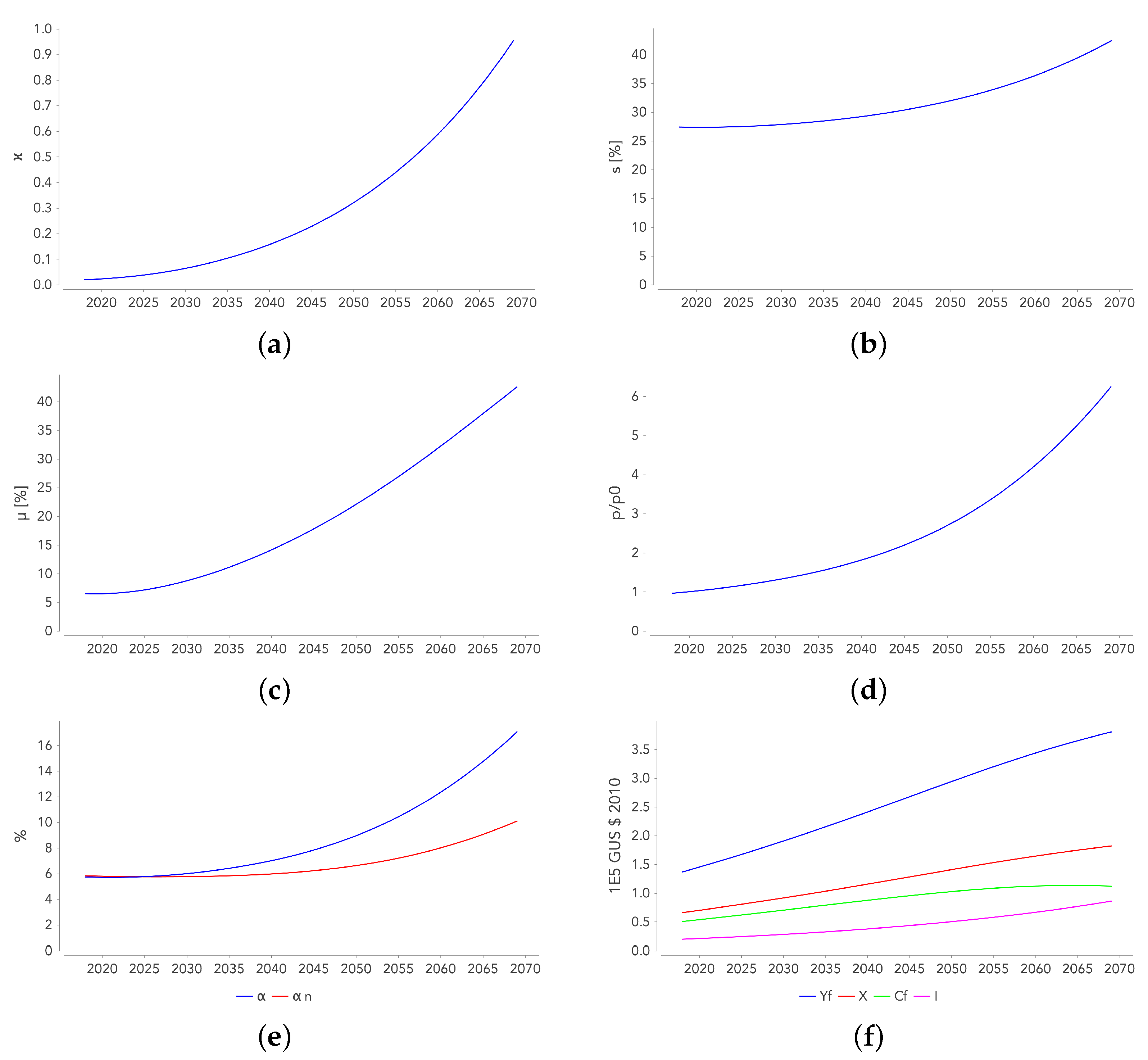
The observations below correspond to an ET that was completed in 2070 with a capital growth rate equal to 3%, under the SD scenario. The TC is chosen to ensure a gradual transition without delay, i.e., a constant weighting rate . TCs that are associated with lower values lead to a “strong” start of the transition followed by a slowdown. TCs that are associated with higher values lead to a delay before the start of the ET.
- Unsurprisingly, the ET results in a significant increase in the real price of energy p (Figure 6d). Despite the decrease of due to technical progress, the growth of the economy results in an increased demand for energy, which pushes up its price. At the end of the ET, the price p reaches six times its initial value. This results contradicts the one of Jacobson [4], claiming that the price of energy will not increase with the ET.
- The rise in the price of energy translates into a significant increase in the share of the ES gross added value in GDP (), as shown in Figure 6e. The increase in the share of the ES net added value in NDP (as measured by ) is more moderate.
- Figure 6f illustrates the evolution of the FS production (), as well as how it is distributed between final consumption , investment I, and intermediate consumption deliveries to the two sectors . While final output remains growing during the transition, there is a decline in the growth of consumption of goods , which, like C, is almost constant at the end of the ET. In other words, because of the increase in the savings rate, the allocation of changes to the detriment of and to the benefit of I (the share of the intermediate consumption deliveries remaining almost constant).
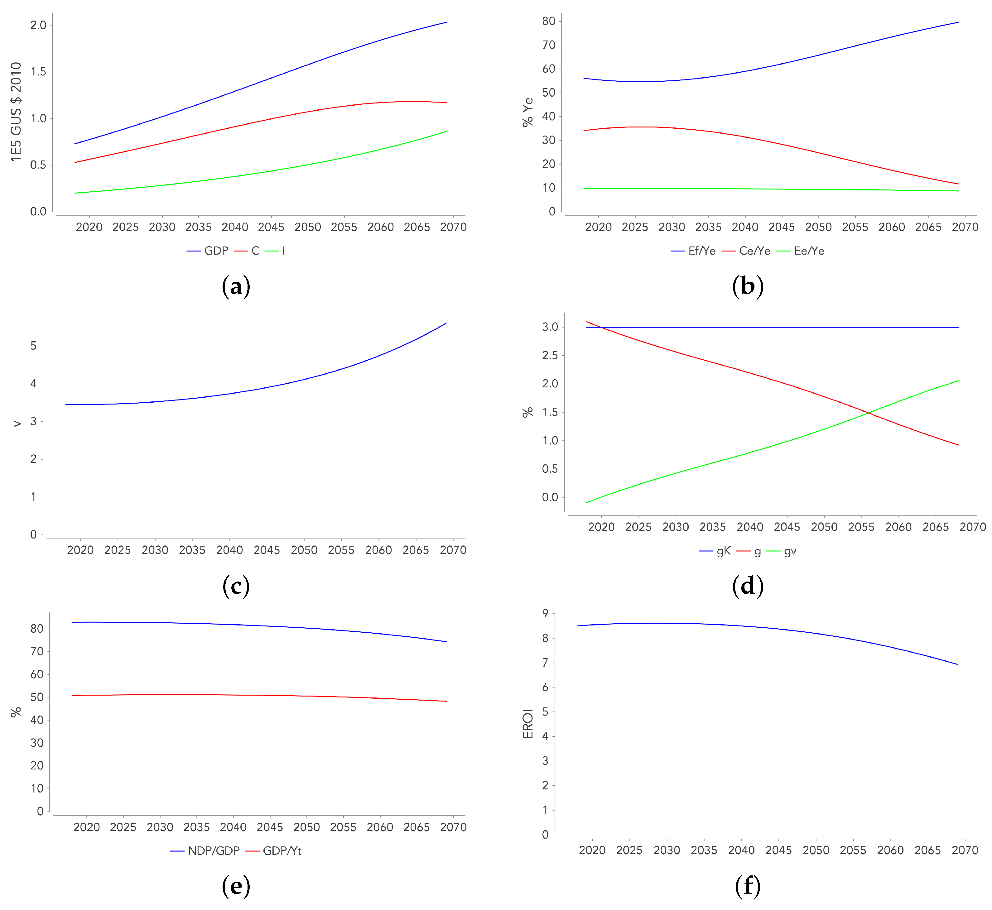
- The increase in s translates into a slowdown in aggregate consumption C with respect to GDP. C becomes quasi-stationary at the end of the ET, while the economy is still growing (Figure 7a).
- Figure 7b illustrates how the ES production is split between self-consumption , deliveries to the FS , and final energy consumption . It can be observed that the share of in increases significantly to the point of taking up most of the energy production at the end of the ET.
- The ET is accompanied by a strong increase in , the ES capital intensity. As the share of capital in the economy that is devoted to this sector continues to grow, the capital intensity of the economy, which is defined as , increases (Figure 7c).
- In Appendix G, we show that the GDP growth is decomposed into the growth of the capital stock and the decline in the capital intensity of the economy (defined as ): . Given the previous observation (v is increasing), the GDP growth rate declines despite the constancy of , as confirmed by Figure 7d.
- Figure 7e illustrates the decrease in the ratios (where denotes the total output of the economy, including all intermediary consumptions) and during the ET. The decrease in the first ratio indicates that the ET results in a faster growth of the intermediary consumptions as compared to GDP (the end-use consumption). The decrease of the second ratio is linked to the increase in the share of capital consumption in GDP, which is induced by the increase in capital intensity v (the increase of v outweighs the decrease of , the latter being due to the fact that the life span of capital is higher in the ES than in the FS). The share of useful production (i.e., for consumption or growth) in total production tends to decrease with the ET.
- Figure 7f shows that the societal point-of-use EROI only slightly decreases during the ET. Several opposing forces are at work: (i) the ET results in an increase of and , which lowers the EROI, (ii) the decrease of increases the EROI, and (iii) the technical progress behind the efficiency gains in the FS increases the EROI.
In conclusion, a strategy aiming at supporting the growth of capital through an increase in the savings rate makes it possible to reach the desired duration for the ET. The price to pay is a slowdown in the growth of total consumption, which ends up stagnating at the end of the transition.
4. Discussion
The simulation results confirm the main findings of the models of the critical literature that are cited in the introduction [9,10,12,13], in particular those presenting the evolution of certain macroeconomic variables in the context of the energy transition [17,19]. It is observed that, if completed in time, the energy transition would be accompanied by a considerable increase in the economy’s savings rate, exceeding 40% in all of the scenarios, as well as in the share of capital that is devoted to the energy sector, rising from less than 10% to more than 40%. At unchanged consumption behaviours (i.e., Exercise 1), the energy transition is almost never completed (except for the SD scenario and a few values of ) because the economy tends towards a stationary state.
In the model of Fagnart et al. [17], the transition is fully completed after a certain period of time, but it is accompanied (with a few exceptions) by a decrease in GDP. This is also the case with the MEDEAS model, where the economy decreases from 2050 onwards in most of the scenarios envisaged [10]. When compared to these general equilibrium models, we are in a partial equilibrium context where the energy demand does not depend on the future evolution of the economy, which might explain why we do not observe a decrease in GDP.
It is important to stress that the obtained results can be considered to be optimistic. Indeed, the underlying assumptions can be considered quite "conservative”; in particular:
- At the beginning of the simulation, the technical progress potential lowering the FS energy intensity is assumed to be significant, since it is (asymptotically) divided by 2. For the BAU scenario, 55% of the gains are obtained in 50 years, and 80% in 100 years. For the SD scenario, most of the gains (97%) are assumed to be obtained before 50 years.
- Production factor intensities (, , and ) of the non-renewable energy subsector are assumed to be constant. However, given the maturity of technologies, technological progress does not seem likely to continue to offset the gradual depletion of resources and the fact that their extraction is becoming increasingly costly in terms of energy and capital. Therefore, a future increase in these intensities seems to be plausible. The same goes for the energy intensity of the renewable subsector (), which is expected to increase with renewable penetration, as modeled in MEDEAS [27].
- Capital is assumed to be perfectly malleable, in the sense that it can move between the non-energy and energy sectors on the one hand, and between the two subsectors of the ES on the other.
- The site selection criterion is a criterion of cost-effectiveness, whether this is measured in energy or economic terms, as indicated in Section 2.3. However, many other factors come into play when setting up a new renewable energy park. This means that, in practice, less profitable sites could be selected before more profitable ones.
Assumptions 1 and 2 explain a large part of the relatively small decrease in EROI during the ET when compared to other models, while, at the same time, the growth rate of the economy declines. Equations (15) and (20) show that the EROI would decrease more if (i) decreased less as a result of lower technical progress potential, (ii) and increased even more as a result of the increase in and , and (iii) increased as a result of the increase of .
Hypothesis 3 allows for reducing a capital stock faster than what its “natural” depreciation rate would allow. It is not applicable if (i) the stock is increasing or (ii) it decreases less quickly than its depreciation rate. Within the framework of the simulations studied, cause (i) is verified for the FS and the renewable energy subsector because their respective stocks are always growing. Cause (ii) applies to the non-renewable energy subsector during much of the ET, but no longer when its end is approaching. Hypothesis 3 then becomes operative and everything happens “as if” thermal power plants were transformed into solar panels or wind turbines, which is, of course, unrealistic.
Removing any of the hypotheses 1 to 4 would complicate the ET and result in its lengthening.
5. Conclusions
This paper develops a modeling scheme articulating a macroeconomic input-output model with two sectors (energy and non-energy) and an energy mode that is able to calculate the maximum potentials of solar and wind energy in order to study the feasibility and pace of the energy transition at the global level. This methodology allows to take two effects into account: a crowding out effect of the non-energy sector in terms of capital allocation, and a location effect due to the declining “quality” of the sites that can receive the additional wind and solar installations.
The main findings obtained thanks to this paper are as follows. At an unchanged savings rate, the transition to a 100% renewable energy system seems unachievable before the end of the century. Controlling energy demand at its current level will drastically reduce the duration of the transition, but it is not enough. The reason lies under the higher capital needs of the renewable energy technologies, resulting in the crowding out of the FS in terms of capital allocation. This effect weighs ever more negatively on growth, slowing down and then blocking the transition in most of the scenarios considered, as the economy tends towards a stationary state.
The strategy aiming at supporting capital growth through an increase in the savings rate allows to counteract the crowding out effect and to reduce significantly the duration of the ET. However, if the demand for energy continues to grow significantly (an increase of 150% by 2100 is expected in the business-as-usual scenario), the transition is only completed after the end of the century. The energy demand should be kept at its current level and the growth rate of capital should be maintained at a value above its historical level in order to allow for a complete transition by 2070. However, because of the significant increase in the savings rate, total consumption ends up stagnating at the end of the transition (while the economy is still growing). On top of that, despite the maintenance of the capital growth rate, the GDP growth rate decreases as a result of the increase in the capital intensity of the economy (as measured by the capital/GDP ratio).
The technical progress affecting the energy intensity of the FS proves to be a fundamental determinant of whether or not the ET is feasible in a finite time. Within the framework of the strategy of the previous point, this intensity must decrease by at least 50% by the end of the ET in 2070.
These results confirm those of the critical literature reviewed in the introduction, in particular concerning the impact of the crowding out effect on growth and the need to control energy demand in order to be able to complete the ET in a sufficiently short period of time.
In order to increase the relevance of the model and to refine the results, several developments are possible. Modelling the non-renewable energy subsector in the same way as what was done for the renewable energy subsector and removing the hypothesis of perfect malleability of capital would contribute to greater realism. Endogenising (i) consumption and investment behaviours and (ii) energy demand would enrich the interactions between the economy and the ET. Taking into account the labour factor next to the capital factor while requiring that their respective remunerations be positive would make it possible to refine the space of allowable trajectories.
Finally it would be interesting to add the cumulative CO emissions to the simulations. Indeed, although we manage, under certain conditions, to complete the transition by 2070, there is no guarantee that the cumulative quantities of CO emitted do not exceed the critical threshold necessary to limit the increase in global temperature.
Author Contributions
All authors have contributed to the different stages. All authors have read and agreed to the published version of the manuscript.
Funding
This research received no external funding.
Conflicts of Interest
The authors declare no conflict of interest.
Abbreviations
The following abbreviations and notations are used in this manuscript:
| ET | energy transition |
| EROI | Energy Return On Investment |
| MM | macroeconomic model |
| EM | energy model |
| ES | energy sector |
| FS | non-energy sector |
| EIC | energy intermediate consumption |
| NEIC | non-energy intermediate consumption |
| units of energy | |
| units of goods produced by the FS | |
| AV | sectoral gross added values |
| NV | sectoral net added values |
| GDP | gross domestic product |
| NDP | net domestic product |
| AS | allowable space |
| TC | transition curve |
| RDM | reduced dynamic model |
| BAU | business-as-usual scenario |
| SD | sustainable development scenario |
| sectoral energy intermediate consumption (EIC) intensities | |
| sectoral capital intensities | |
| sectoral non-energy intermediate consumption (NEIC) intensities |
Appendix A. The Societal EROI
Point-of-use EROI is defined as follows:
In order to produce an amount of energy , the ES consumes as EIC (i.e., direct energy consumption) (in ), as NEIC, and uses a stock of capital .
Since the EROI only accounts for energy flows, it is necessary to estimate the embodied energy included in the indirect energy inputs, i.e., the intermediate consumption flow and capital stock . As annual flows are considered in the model, we take into account the capital depreciation in the denominator of the EROI. The capital flow in the denominator of the EROI is estimated as the energy content of , i.e., all the energy that was required to produce, install, maintain and dismantle the fraction of the ES capital stock consumed during the period under consideration. This estimate is therefore based on the energy content of the share of the investment (at time t) used to replace the capital that has become obsolete (at time t). An alternative approach would have been to estimate the embodied energy in the capital stock based on the energy content of past investments. Since decreases over time, this approach would lead to a higher estimate of the embodied energy contained in the flow measuring capital depreciation.
Let and (both in ) be the energy embodied in the flows measuring NEIC and capital depreciation . Since (i) the production of the FS is assumed to be homogeneous and (ii) it takes unit of energy to produce one unit of good, this embodied energy flow can be estimated by:
given Equations (1) and (15). The energy delivered (i.e., the amount that reaches the FS plus the amount used for final consumption) is defined as the gross energy produced , minus the direct energy inputs . The EROI then becomes:
One finds Equation (20).
Appendix B. Site Selection Criteria
In the EM, it is considered that the sites with the best EROI will be chosen first. For this approach to be economically consistent, this criterion must be the same as the criterion of selecting the sites with the highest profits.
For the renewable technologies of interest here (wind and solar), (i) the energy intensity of an installation is the same for all sites considered, (ii) the capital required and the maintenance costs included in are fixed costs, which are not site-dependent.
In view of the above, the profits related to sites a and b for a given technology are written:
Profits per unit of energy produced are then written:
If , then necessarily , which implies (while ).
Now, the point-of-use EROIs of the two sites are written respectively (from Equation (20)):
It follows that .
Appendix C. Interval for p
Criterion defined in Equation (24) requires that the net sectoral added values are both positive. With Equations (9) and (13), criterion NV translates into the following inequality:
With Equations (10) and (14), criterion NV translates into the following inequality:
which implies and hence the following allowable interval for p:
can be transformed into an interval for but this will depend on assumptions made about the parameters, in particular the behavioural parameters s (or ) and .
Appendix D. Calculation of the Allowable Spaces
Thereafter, the allowable range for the ratio is established for the 2 exercises, as well as the equation that links and k with (Exercise 1) or s (Exercise 2).
Appendix D.1. Preliminaries
For the developments that will follow, let us define , the final demand to the FS.
By the expenditure approach of GDP, we have:
Hence the following relationship between GDP, , and s (useful for Exercise 1):
And, as , the following relationship between C, , I and (useful for Exercise 2):
Appendix D.2. Exercise 1—k Interval
With Equations (18), (19), (A4)–(A6), p is expressed as a function of the technical parameters and the outputs :
Let , then the last equality becomes:
As a result, and with , , and , Equation (A3) becomes:
⇒
⇒
⇒
⇒
To corresponds an interval for k. Indeed, k and y are linked by:
Therefore, we have:
These bounds are increasing functions of (since , and thus , and ), and decreasing functions of .
Indeed, the EM results show that solar and wind power are more intensive in goods produced by the FS than the technologies they replace. It should also be noted that the lower the energy intensity of the FS , the higher the envelopes are in the space.
Appendix D.3. Exercise 1—Capital Growth Rate
Yet Equation (A6) gives:
Substituting by Equation (A4), one finds:
The first term is an increasing function of k, and is an increasing function of k if , and negative otherwise. It follows that is an increasing function of k if is not too high.
Appendix D.4. Exercise 2—k Interval
Given Equations (A7) and (19) (which gives ):
Equation (A10) gives an expression for I (). Combined with Equations (A7) and (A5) the previous equation becomes:
With notations , , , Equation (A3) becomes:
Both the numerator and the denominator are positive, so the inequality rewrites as follows:
Which gives two inequalities:
If , or if is not too high, the left-hand side of the first inequality is positive, which implies that the other members of the 2 inequalities are also positive (because ). Hence the following interval is found for k:
Or equivalently:
Appendix D.5. Exercise 2—Savings Rate
In addition, with Equation (A4) we have:
As a result we find an expression for s as a function of the technical parameters, , , k (and ):
Appendix E. Historical Evolution of v, xf and vf
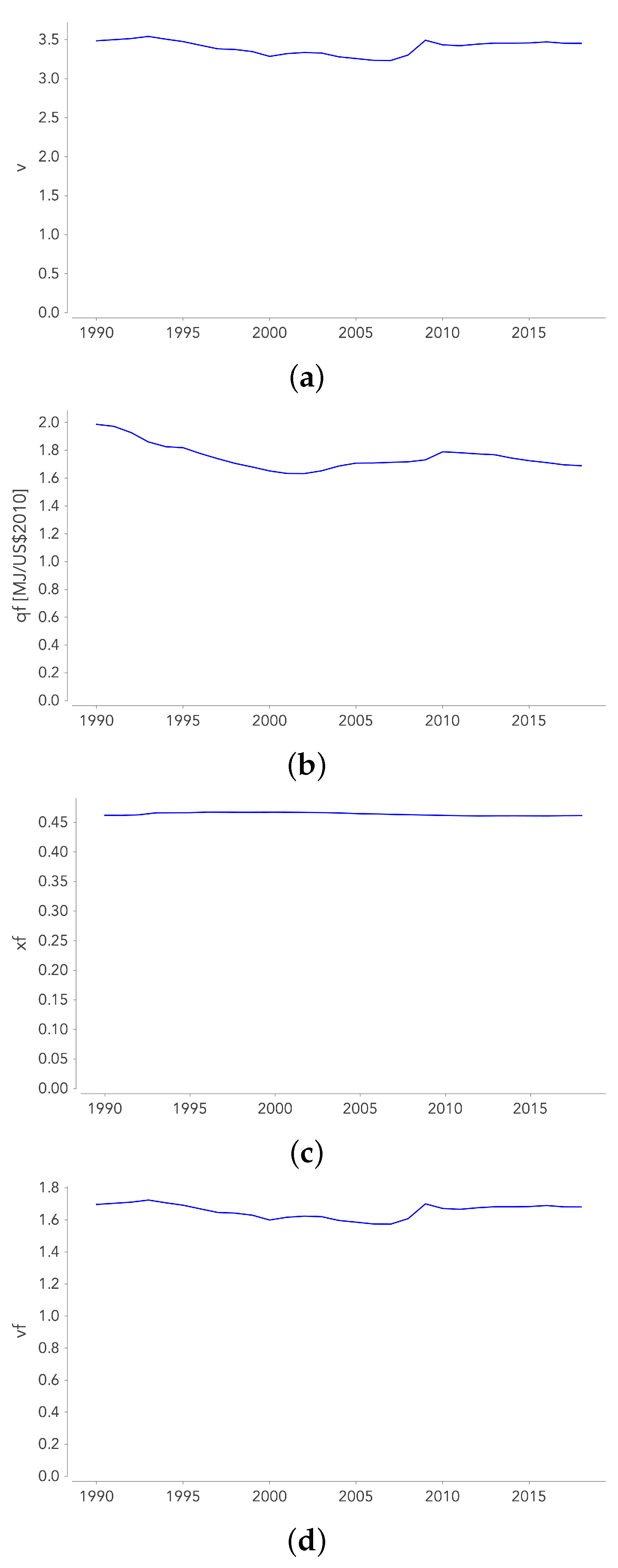
Starting from the estimation of the total capital stock for the reference year (), and with historical data regarding the total GDP and savings rate s, we find capital stock estimates from the time period 1990–2018.
With theses estimates for and the observed data for the GDP and savings rate the historical evolution of v is estimated. Then thanks the calibration procedure developed by Dupont et al. [24] and the yearly estimations of K and v, the historical evolution of the technical parameters of the FS can be retraced. These are shown in Figure A1. While has decreased by an average of 0.8% per year over the last 30 years, v, and have not seen any significant change.
Figure A1.
Historical evolution of: (a): the capital intensity of the economy (i.e., the capital/GDP ratio), (b): , the energy intensity of the FS, (c): , the NEIC intensity of the FS and (d): , the capital intensity of the FS.
Figure A1.
Historical evolution of: (a): the capital intensity of the economy (i.e., the capital/GDP ratio), (b): , the energy intensity of the FS, (c): , the NEIC intensity of the FS and (d): , the capital intensity of the FS.

Appendix F. Future Evolution of Ye and qf
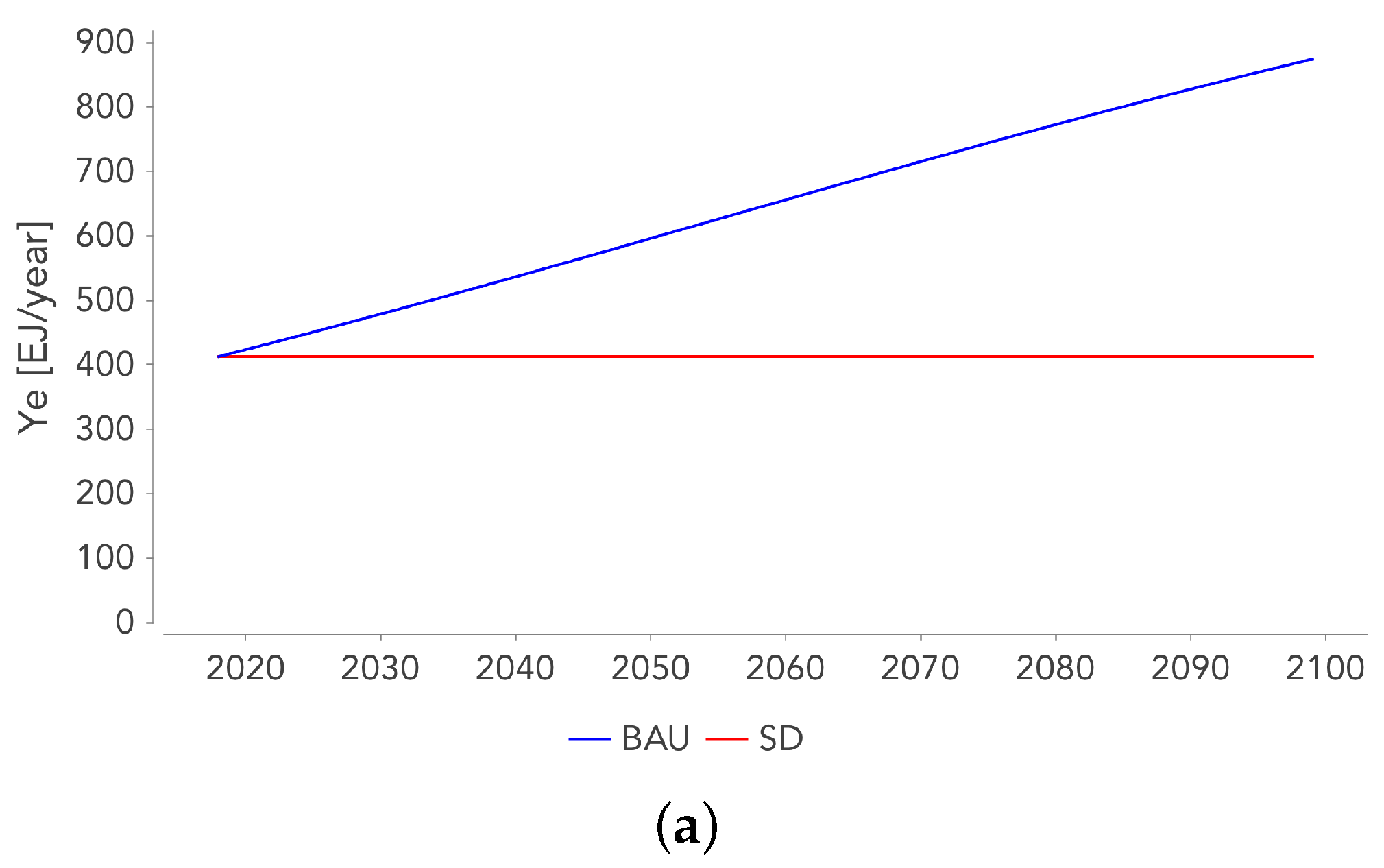
We consider 2 scenarios for the future evolution of the energy demand and the energy intensity of the FS. The first scenario is the business as usual scenario (BAU), which is an extrapolation of past trends of and (see Table A1). The second scenario is based on the sustainable development (SD) scenario of the IEA “World Energy Outlook” report ([25]). It represents an accelerated energy transition in order to achieve sustainable development goals in terms of energy access (universal access to modern energy by 2030), climate change (limiting the average temperature increase to below 2 °C) and air quality (significant reduction in air pollution-related deaths).
For BAU, extrapolating the annual growth rates observed over the period 1990–2018 (see Table A1), we obtain for 2040: , and .

Table A1.
Historical annual growth rates of and .
| 1990–2018 | 1990–1999 | 2000–2009 | 2010–2018 | |
|---|---|---|---|---|
| [%] | 1.63 | 1.02 | 2.05 | 1.16 |
| [%] | −0.58 | −1.85 | 0.56 | −0.72 |
The IEA SD scenario assumes a energy consumption for 2040 similar to today, and a higher annual rate of decline in the energy intensity of the economy than has been observed in the past. The IEA considers an annual decline rate for the primary energy intensity of GDP of 3.5%. Since only final energy is considered here, the rate of decrease of will be lower. If we consider an annual decrease rate of 2.25% (a rate never observed over the 1990–2018 period), we find .
In the long term, asymptotic values are given for and , which are and . For BAU, , while for SD, . For both scenarios, .
The evolution of is estimated as follows:
which assumes that the difference between the initial value of and its limit value () decreases exponentially. Knowing in 2040, we can estimate , the rate of change of the gap from to its stationary value . In the BAU framework, the evolution of is modelled according to a logistic curve:
The rate is calibrated iteratively, starting from the value of in 2040.
The values of and for the two scenarios are shown in Table A2. The corresponding temporal evolutions of and are shown in Figure A2.
Table A2.
Calculated values of and for both scenarios.
| [%] | [%] | |
|---|---|---|
| BAU | 2.72 | 1.6 |
| SD | 0 | 7 |
Figure A2.
Future evolution of Ye and qf for the 2 scenarios: (a): Ye(t), (b): qf(t), (c): qf(t)/qf0.
Figure A2.
Future evolution of Ye and qf for the 2 scenarios: (a): Ye(t), (b): qf(t), (c): qf(t)/qf0.


Appendix G. Link between v, g and gk
Using Equations (3), (17) and the definiton of the capital intensity of the economy () we write:
Hence the capital growth rate is given by:
Be g the GDP growth rate: . One can write at first order , which implies:
It shows that GDP growth is decomposed into the growth of the capital stock and the decline in the capital intensity of the economy.
References
- Budischak, C.; Sewell, D.; Thomson, H.; Mach, L.; Veron, D.E. Cost-minimized combinations of wind power, solar power and electrochemical storage, powering the grid up to 99.9% of the time. J. Power Sources 2013, 225, 60–74. [Google Scholar] [CrossRef] [Green Version]
- Ellabban, O.; Abu-rub, H.; Blaabjerg, F. Renewable energy resources: Current status, future prospects and their enabling technology. Renew. Sustain. Energy Rev. 2014, 39, 748–764. [Google Scholar] [CrossRef]
- Jacobson, M.Z.; Delucchi, M.A.; Bazouin, G.; Bauer, Z.A.F.; Heavey, C.C.; Fisher, E.; Morris, S.B.; Piekutowski, D.J.Y.; Vencill, T.A.; Yeskoo, T.W. Environmental Science the 50 United States. Energy Environ. Sci. 2015, 8, 2093–2117. [Google Scholar] [CrossRef]
- Jacobson, M. 100% Clean and Renewable Wind, Water, and Sunlight All-Sector Energy Roadmaps for 139 Countries of the World. Joule 2017, 1, 108–121. [Google Scholar] [CrossRef] [Green Version]
- Jacobson, M.Z. Roadmaps to Transition Countries to 100% Clean, Renewable Energy for All Purposes to Curtail Global Warming, Air Pollution, and Energy Risk. Earth’s Futur. 2017, 5, 948–952. [Google Scholar] [CrossRef]
- Davis, S.J.; Lewis, N.S.; Shaner, M.; Aggarwal, S.; Arent, D.; Azevedo, I.L.; Benson, S.M.; Bradley, T.; Brouwer, J.; Chiang, Y.M.; et al. Net-zero emissions energy systems. Science (80-.) 2018, 360. [Google Scholar] [CrossRef] [Green Version]
- Ram, M.; Bogdanov, D.; Aghahosseini, A.; Gulagi, A.; Oyewo, A.; Child, M.; Caldera, U.; Sadovskaia, K.; Farfan, J.; Barbosa, L.; et al. Global Energy System Based on 100% Renewable Energy-Power, Heat, Transport and Desalination Sectors; Lappeenranta University of Technology and Energy Watch Group: Lappeenranta, Finland; Berlin, Germany, 2019. [Google Scholar]
- Bogdanov, D.; Gulagi, A.; Fasihi, M.; Breyer, C. Full energy sector transition towards 100% renewable energy supply: Integrating power, heat, transport and industry sectors including desalination. Appl. Energy 2021, 283, 116273. [Google Scholar] [CrossRef]
- Moriarty, P.; Honnery, D. Feasability of a 100% Global Renewable Energy System. Energies 2020, 13, 5543. [Google Scholar] [CrossRef]
- Capellán-Pérez, I.; de Blas, I.; Nieto, J.; de Castro, C.; Miguel, L.J.; Carpintero, O.; Mediavilla, M.; Lobejon, L.F.; Ferreras-alonso, N.; Rodrigo, P.; et al. MEDEAS: A new modeling framework integrating global biophysical and socioeconomic constraints. Energy Environ. Sci. 2020. [Google Scholar] [CrossRef]
- WWF. The Energy Report 100% Renewable by 2050; Technical Report; WWF: Gland, Switzerland, 2011. [Google Scholar]
- Nieto, J.; Miguel, L.J.; Blas, I.D. Macroeconomic modelling under energy constraints: Global low carbon transition scenarios. Energy Policy 2020, 137. [Google Scholar] [CrossRef] [Green Version]
- Sers, M.R.; Victor, P.A. The Energy-emissions Trap. Ecol. Econ. 2018, 151, 10–21. [Google Scholar] [CrossRef]
- Dupont, E.; Jeanmart, H.; Possoz, L.; Fagnart, J.F.; Germain, M. Transition Énergétique et (dé) Croissance Économique; Université Catholique de Louvain, Institut de Recherches Economiques et Sociales (IRES): Ottignies-Louvain-la-Neuve, Belgium, 2017. [Google Scholar]
- Dale, M.; Krumdieck, S.; Bodger, P. Global energy modelling—A biophysical approach (GEMBA) Part 1: An overview of biophysical economics. Ecol. Econ. 2012, 73, 152–157. [Google Scholar] [CrossRef]
- Dale, M.; Krumdieck, S.; Bodger, P. Global energy modelling—A biophysical approach (GEMBA) Part 2: Methodology. Ecol. Econ. 2012, 73, 158–167. [Google Scholar] [CrossRef]
- Fagnart, J.F.; Germain, M.; Peeters, B. Can the Energy Transition Be Smooth? A General Equilibrium Approach to the EROEI. Sustainability 2020, 12, 1176. [Google Scholar] [CrossRef] [Green Version]
- Court, V.; Jouvet, P.A.; Lantz, F. Long-term endogenous economic growth and energy transitions. Energy J. Int. Assoc. Energy Econ. 2018, 39. [Google Scholar] [CrossRef]
- Režný, L.; Bureš, V. Energy Transition Scenarios and Their Economic Impacts in the Extended Neoclassical Model of Economic Growth. Sustainability 2019, 11, 3644. [Google Scholar] [CrossRef] [Green Version]
- Rye, C.D.; Jackson, T. A review of EROEI-dynamics energy-transition models. Energy Policy 2018, 122, 260–272. [Google Scholar] [CrossRef]
- Dupont, E.; Koppelaar, R.; Jeanmart, H. Global available wind energy with physical and energy return on investment constraints. Appl. Energy 2018, 209, 322–338. [Google Scholar] [CrossRef]
- Dupont, E.; Koppelaar, R.; Jeanmart, H. Global available solar energy under physical and energy return on investment constraints. Appl. Energy 2020, 257, 113968. [Google Scholar] [CrossRef]
- Fagnart, J.F.; Germain, M. Net energy ratio, EROEI and the macroeconomy. Struct. Chang. Econ. Dyn. 2016, 37, 121–126. [Google Scholar] [CrossRef]
- Dupont, E.; Germain, M.; Jeanmart, H. Estimate of the Societal Energy Return on Investment (EROI). Biophys. Econ. Sustain. 2021, 6. [Google Scholar] [CrossRef]
- IEA. World Energy Outlook 2020; Technical Report; IEA: Paris, France, 2020. [Google Scholar]
- EIA. Annual Energy Outlook 2020; EIA: Washington, DC, USA, 2020. [Google Scholar]
- Capellán-Pérez, I.; de Blas, I.; Nieto, J.; de Castro, C.; Miguel, L.J.; Mediavilla, M.; Carpintero, O.; Rodrigo, P.; Frechoso, F.; Cáceres, S. Guiding European Policy toward a Low-Carbon Economy. Modelling Sustainable Energy System Development under Environmental and Socioeconomic Constraints. D4.1 (D13) Global Model: MEDEAS-World Model and IOA Implementation ot Global Geographical Level; Technical Report; Pg. Marítim de la Barceloneta: Barcelona, Spain, 2017. [Google Scholar]
- OECD. Input-Output Tables; OECD: Paris, France, 2015. [Google Scholar]
- Kümmel, R.; Lindenberger, D.; Weiser, F. The economic power of energy and the need to integrate it with energy policy. Energy Policy 2015, 86, 833–843. [Google Scholar] [CrossRef]
- Ayres, R.U.; van den Bergh, J.C.J.M.; Lindenberger, D.; Warr, B. The underestimated contribution of energy to economic growth. Struct. Chang. Econ. Dyn. 2013, 27, 79–88. [Google Scholar] [CrossRef]
- Court, V.; Fizaine, F. Energy expenditure, economic growth, and the minimum EROI of society. Energy Policy 2016, 95, 172–186. [Google Scholar] [CrossRef]
- IPCC. Global Warming of 1.5 °C; Technical Report; Intergovernmental Panel on Climate Change: Geneva, Switzerland, 2018. [Google Scholar]
- IEA. Key World Energy Statistics 2020; Technical Report August; IEA: Paris, France, 2020. [Google Scholar]
Figure 1.
Diagram of the economy, closed and with two sectors: the ES producing energy, and the FS producing general-purpose goods. represent the output flows, represent the intermediate consumptions of energy (EIC), the non-energy intermediate consumptions (NEIC), and the stocks of capital used by each sector.

Figure 2.
The evolution of the technical parameters of the renewable energy subsector as a function of , the amount of renewable energy produced (in exajoules produced per year): (a): , (b): .
Figure 2.
The evolution of the technical parameters of the renewable energy subsector as a function of , the amount of renewable energy produced (in exajoules produced per year): (a): , (b): .

Figure 3.
Representation of the AS and of a TC, for a fictitious scenario with and being fixed. The solid curves represent the bounds of the interval for k (Equation (28)), and the AS is the space between these two curves. The dashed curve shows a particular TC and the dots show the trajectory of the ET, thus the discrete pairs for a few successive years.

Figure 4.
Evolution of the technical parameters of the ES as a function of the penetration rate ( corresponds in this case to ): (a): , (b): , (c): .
Figure 4.
Evolution of the technical parameters of the ES as a function of the penetration rate ( corresponds in this case to ): (a): , (b): , (c): .

Figure 5.
Exercise 1, evolution as a function of of: (a): , (b): the asymptotical value , and, only for the SD scenario and , (c): the year of the end of the transition , and (d): the residual capital growth rate.
Figure 5.
Exercise 1, evolution as a function of of: (a): , (b): the asymptotical value , and, only for the SD scenario and , (c): the year of the end of the transition , and (d): the residual capital growth rate.

Figure 6.
Temporal evolution of economic variables for Exercise 2, scenario SD, with = 3% and = 0.418. (a): the renewable penetration rate , (b): the savings rate , (c): the share of capital stock devoted to the ES , (d): the energy price compared to its price in 2018 , (e): the share of the ES gross added value in GDP (blue curve), and the share of the ES net added value in NDP (red curve), and (f): the FS output and its distribution: NEIC , final consumption and investment

Figure 7.
Temporal evolution of economic variables for Exercise 2, scenario SD, with = 3% and = 0.418 (continuation and end). (a): the gross domestic product GDP(t) and its distribution between consumption and investment , (b): the distribution of the ES output , in relative terms, between self-consumption (), deliveries to the FS (), and final energy consumption (), (c): the capital intensity of the economy (i.e., the capital/GDP ratio) , (d): the capital growth rate (constant) and its distribution between the GDP growth rate (decreasing) and the growth rate of the capital intensity of the economic (increasing), (e): the ratios of the GDP to the total output of the economy (defined as ) (blue curve), and the ratio between the NDP and GDP (red curve), and (f): the point-of-use societal EROI, EROI.

Table 1.
The calibration of the technical parameters and of the EROI for the reference year (2018).
| [-] | 1.72 |
| [MJ/US$ 2010] | 1.7 |
| [-] | 0.47 |
| [US$2010/(GJ/y)] | 39.07 |
| [%] | 9.8 |
| [US$2010/GJ] | 3.32 |
| EROI [-] | 8.5 |
Table 2.
An estimation of the technical parameters of both subsectors of the ES in 2018, corresponding to a penetration rate of 2%.
Table 2.
An estimation of the technical parameters of both subsectors of the ES in 2018, corresponding to a penetration rate of 2%.
| Energy Sector | Non-Renewable Subsector | Renewable Subsector | |
|---|---|---|---|
| [%] | 9.76 | 9.78 | 8.68 |
| [US$2010/GJ] | 3.32 | 3.32 | 3.01 |
| [US$2010/(GJ/y)] | 39.07 | 26.65 | 647.63 |
Table 3.
Exercise 2: values for and of , s (in 2050, 2100 and ) and , for the two scenarios.
| BAU | SD | |||||||||
|---|---|---|---|---|---|---|---|---|---|---|
| 2050 | 2100 | 2129 | 2050 | 2100 | 2133 | 2050 | 2085 | 2050 | 2090 | |
| [%] | 16.8 | 46.1 | 100 | 0 | 17 | 100 | 31.2 | 100 | 0 | 100 |
| s [%] | 29.8 | 34.8 | 44 | 24.4 | 25.9 | 41.1 | 30.7 | 40.1 | 23.9 | 36.8 |
Table 4.
Minimum capital growth rate for a transition completed by 2070 (Exercise 2, scenario SD), and the corresponding savings rate at the end of the ET.
Table 4.
Minimum capital growth rate for a transition completed by 2070 (Exercise 2, scenario SD), and the corresponding savings rate at the end of the ET.
| [%] | [%] | |
|---|---|---|
| 0 | 2.91 | 43.5 |
| 0.2 | 2.96 | 43.1 |
| 0.4 | 3 | 42.5 |
| 0.6 | 3.04 | 42 |
| 0.8 | 3.08 | 41.5 |
| 1.0 | 3.12 | 41.1 |
Publisher’s Note: MDPI stays neutral with regard to jurisdictional claims in published maps and institutional affiliations. |
© 2021 by the authors. Licensee MDPI, Basel, Switzerland. This article is an open access article distributed under the terms and conditions of the Creative Commons Attribution (CC BY) license (https://creativecommons.org/licenses/by/4.0/).
Share and Cite
MDPI and ACS Style
Dupont, E.; Germain, M.; Jeanmart, H. Feasibility and Economic Impacts of the Energy Transition. Sustainability 2021, 13, 5345. https://0-doi-org.brum.beds.ac.uk/10.3390/su13105345
AMA Style
Dupont E, Germain M, Jeanmart H. Feasibility and Economic Impacts of the Energy Transition. Sustainability. 2021; 13(10):5345. https://0-doi-org.brum.beds.ac.uk/10.3390/su13105345
Chicago/Turabian StyleDupont, Elise, Marc Germain, and Hervé Jeanmart. 2021. "Feasibility and Economic Impacts of the Energy Transition" Sustainability 13, no. 10: 5345. https://0-doi-org.brum.beds.ac.uk/10.3390/su13105345
Note that from the first issue of 2016, this journal uses article numbers instead of page numbers. See further details here.