
Including Urban Heat Island in Bioclimatic Early-Design Phases: A Simplified Methodology and Sample Applications


Department of Architecture and Design, Politecnico di Torino, 10125 Turin, Italy
*
Author to whom correspondence should be addressed.
Sustainability 2021, 13(11), 5918; https://0-doi-org.brum.beds.ac.uk/10.3390/su13115918
Submission received: 27 April 2021
/
Revised: 18 May 2021
/
Accepted: 18 May 2021
/
Published: 24 May 2021
(This article belongs to the Special Issue Urban Climate, Comfort and Building Energy Performance in the Mediterranean Climate)
Abstract
:Urban heat island and urban-driven climate variations are recognized issues and may considerably affect the local climatic potential of free-running technologies. Nevertheless, green design and bioclimatic early-design analyses are generally based on typical rural climate data, without including urban effects. This paper aims to define a simple approach to considering urban shapes and expected effects on local bioclimatic potential indicators to support early-design choices. Furthermore, the proposed approach is based on simplifying urban shapes to simplify analyses in early-design phases. The proposed approach was applied to a sample location (Turin, temperate climate) and five other climate conditions representative of Eurasian climates. The results show that the inclusion of the urban climate dimension considerably reduced rural HDD (heating degree-days) from 10% to 30% and increased CDD (cooling degree-days) from 70% to 95%. The results reveal the importance of including the urban climate dimension in early-design phases, such as building programming in which specific design actions are not yet defined, to support the correct definition of early-design bioclimatic analyses.
1. Introduction
According to the UN’s World Urbanization Prospects (2018) [1], the proportion of the global population living in urban areas is higher than that of rural areas, with a ratio of 55% in 2018. This ratio is growing continuously; it was only 30% in 1950 and is expected to reach 68% by 2050. Similarly, several research studies have underlined the impact that large cities have on local climate and local environmental parameters. For example, Oke et al. analyzed the urban impact on physical parameters, including temperature, humidity, precipitations, airflows, thermal and radiative exchanges, considering the whole energy balance at a local scale [2]. Similarly, Beckers et al. focused on radiative exchanges and radiative balances in urban contexts, introducing complex physical and geometrical models [3]. Moreover, Erell et al. focused on analyzing outdoor thermal comfort and environmental issues connected to urban spaces [4].
Hence, the urban heat island (UHI) effect is a phenomenon that impacts local urban conditions more so than rural climates, which affects local temperature profiles, as mentioned by Oke [5]. UHI has a significant impact on cooling energy consumptions of buildings located in urban areas compared to rural ones, as suggested by Santamouris and colleagues [6,7]. Additionally, Dong et al. underlined the impact of UHI on physical discomfort in summer due to changes in environmental parameters [8].
These effects are more evident in large dense urban areas impacting their inhabitants. Cities, especially larger ones, are characterized by specific microclimate conditions compared to rural sites, as detailed by the work of Yang and Chen [9], which was based on differences in boundary conditions. Furthermore, in megacities, such as Beijing, it was demonstrated that, in 2015, a main heat island effect occupied more than 79.85% of the total urban area, and this percentage was continuously expanding, such as recently underlined by UN [10]. According to the UN definition, there are 33 megacities globally, i.e., cities exceeding 10 million inhabitants, while another 10 are expected to become megacities by 2030 [11]. As the majority of humans live in an urban environment, the study of urban microclimate constitutes an essential challenge for guaranteeing the comfort of city inhabitants; the management and mitigation of climatic risks, especially at the urban level (e.g., urban heat islands); the reduction in energy needs by the building stock, including the urban-driven effects on buildings and outdoor open spaces. A need to consider urban effects in local climate is hence important for correctly defining bioclimatic choices.
Several studies have tried to investigate the correlation between urban morphology and UHI [12,13,14,15]. Jin et al. selected three urban morphological parameters to create a multilinear regression model to predict air temperature in Singapore [12]. In other research, specific parameters have been examined and proposed, e.g., the capacity and building-scale energy indicator suggested by Grifoni et al. [13], or building material properties and green infrastructure, such as those included in the analyses by Palme et al. [14,15]. These studies proved that urban morphologies—synthesized by averaged morphological parameters at urban or large district scales—have a high impact on simulated building performance. However, the urban effect considered in these studies was discussed concerning detailed buildings and advanced design stages. Detailed building models are designed to support simulations without focusing on the early-design phases, such as building programming in which early-bioclimatic analyses and choices are defined. It is, nevertheless, underlined that, in bioclimatic design approaches, early-design analyses based on local climate evaluations are an essential step for supporting appropriate design choices and improving further design stage climate performances [16,17].
Other researchers have developed abstract models to represent the real urban context for climate simulation, considering the UHI impact at the local climate scale rather than at the sub-site level [18,19]. Salvati et al. and Morganti et al. used normalized models to represent different urban textures to analyze potential relationships between urban morphological indicators with respect to building energy demands and solar availability [18,19]. The simplified urban models adopted in these studies were based on abstractions of the existing urban fabric and were further coupled with detailed simulations on specific buildings. Focusing on urban forms and their climate impact, archetypal build forms can be used to simplify and resemble actual complex urban environments and analyze the environmental performance of different urban morphologies. Ratti et al. studied the environmental variables of three different urban forms in a hot-arid climatic context. The urban forms were from traditional Arab courtyards and two potential modern urban variations; the results showed that courtyard configuration affected their performance in the specific climatic context [20].
Similarly, basic principles of energy and comfort performances in an urban environment have been proposed by several researchers; for example, Erell et al. discussed the principle of integration climate analysis in the urban planning process, underlining the large impact of changes in climate conditions at urban sites compared to rural ones [4]. The same research group correlated simple city-block diagrams—both simulated and modeled at a real site—to analyze the impact of bioclimatic strategies on outdoor urban contexts [21]. Similar simplified block-city models have been used to support several analyses in high-density cities considering thermal comfort, ventilation, and daylight, which are recognized as essential issues to be considered in sustainable city development at all design stages—for example, the design approach for high-density cities reported by Ng [22]. The pre-assessment of urban simplified block-city morphologies has been recognized as a useful tool in bioclimatic early-design stages. In particular, Chokhachian et al. suggested a generative approach to identify performative urban design solutions that give design suggestions on urban forms for determining urban densities to achieve higher performance in terms of UHI, solar access, and daylight [23]. Lima et al. analyzed the thermal loads between two architectural configurations of an office building in different environmental settings in a hot and humid climate [24].
Additionally, Salvati et al. explored the building energy demand in a Mediterranean climate with different urban compactness and showed that the compact urban textures with a site coverage ratio above 0.5 are more energy efficient on an annual basis [18]. Other studies have introduced models, tools, and approaches with different levels of complexity to define the urban impact on climate files. Begüm Sakar and Olgu Çalışkan introduced parametric modeling of three typological urban form variations based on a transposition to cuboid forms of real urban fabrics; they adopted a Grasshopper and a simplified internal sky-view factor calculator to support correlations with UHI magnitude defined with the simple expression proposed by Oke [25]. Differently, the paper of Palme et al. supported the definition of a simplified methodology to downscale the urban climate to include UHI impacts at the building simulation level—detailed building design stage by adopting Urban Weather Generator (UWG) and TRNSYS simulations [26]. A consistent update of this approach was proposed by Salvati et al., defining a methodology to include the impact of UHI on detailed dynamic building simulations, considering the effects of urban morphologies on temperature, relative humidity, radiation exchanges, and wind velocities in urban canyons [27]. Both studies underline that it is important to use UHI-morphed weather files to correctly define advanced energy simulations of buildings at advanced design stages in urban contexts.
Although more studies are needed to underline the impacts of urban archetypal forms on local climate conditions defining simplified methodologies can be applied since early-design phases, including the urban-heat-island dimension in green and sustainable design from building programming. Building programming is the early-design phase in which it is possible to influence more building design processes at a lower cost. In this first early-design step, the specific building shape is not yet fully defined, allowing for high flexibility and the possibility of impacting the project definition when cumulative costs are limited, such as defined in several works on design instrument and approach maturity, e.g., BIM (Building Information Modelling) and green-design methodologies [28,29,30,31,32]. The possibility of including the UHI phenomenon in the local climate to support more coherent early-bioclimatic analyses is very important; even if simple methods, tools, and parameters are considered, it is not possible at this design stage to develop detailed building simulations. This paper aims to introduce a simple approach to connecting urban archetypal forms with bioclimatic KPIs (Key Performance Indicators), including urban shape influences on typical climatic conditions to support early-design phases.
Paper’s Objectives and Structure
The proposed paper introduces a simple methodology to consider the general impact of urban morphologies and urban heat islands (UHIs) on typical climate conditions to support early-design bioclimatic choices. The main objective considered was as follows:
- Furthermore, the following specific objectives were also pursued:
- To underline the importance in considering, from early-design phases, the urban dimension in local typical weather conditions during climate analyses due to the high impact of urban morphologies with respect to rural sites via sample case studies;
- To analyze the influence of urban morphed climate on early-design bioclimatic key performance indicators (KPIs), i.e., local heating and cooling degree days/hours (HDD/H, CDD/H), bioclimatic comfort hour calculations using bioclimatic charts, solar analyses (the number of sun-exposed hours), and the local climatic potential of low-energy cooling techniques, adopting sample case studies;
- To compare urban morphological effects on six sample locations characterized by different climatic conditions.
Section 1 is devoted to the paper introduction (state of the art and objectives). The rest of the paper is as follows: Section 2 contains the methodology, which introduces and details the proposed methodology for defining UHI impacts on local climate due to urban morphologies, including the description of adopted KPIs; Section 3 contains the results, from applying the given methodology to a sample case study (Turin, Italy—Cfa climate zone) in order to verify the impact of UHI on adopted KPIs and illustrate a sample application of the methodology; Section 4 contains a discussion of the ability of the assumed urban spatial configuration models to represent real urban spatial configurations when input data are defined for climate morphing, and comparing the impact of UHI on a set of different locations characterized by representative climatic conditions in Eurasian areas to demonstrate that the methodology may be applied in different contexts and that results are local-specific. Section 4 also includes a discussion of the main limitations of this study. Finally, Section 5 reports the paper’s conclusions.
2. Methodology
The adopted methodology can be subdivided into the following list of processes: i: the definition of urban morphological data (Section 2.1); ii: the calculation of UHI impact on local air temperature and humidity (Section 2.2) by morphing typical meteorological year (TMY) databases; iii: the calculation of early-design climatic KPIs assessing the urban-morphological impact on energy-climate indicators (Section 2.3) and the applicability potential of different bioclimatic and low-energy technologies (Section 2.4). Finally, the description of the chosen set of climate case studies is introduced Section 2.5).
2.1. Urban Morphological Data
This paper aims to introduce a simple methodology able to be adopted in the early-design phases by architects for supporting green design choices (e.g., bioclimatic ones, such as defined in historic [16,37] and recent publications [17]) before the detailed definition of a building and a fully defined model for advanced simulations. A simplified approach was developed to consider the effects of different urban compound shapes on local bioclimatic potential analyses. Urban shapes were approached adopting representative configurations able to translate real spaces into archetype forms, in line with previous studies of other authors, as mentioned in Section 1.
A set of four representative urban spatial configurations (district scale) (Figure 1) were adapted from the literature of urban morphologies, with special regard to the typological shapes introduced by Ratti et al. [20]. The four forms were derived in this study to represent real building compounds at a climate-influencing scale and were translated into the GrasshopperTM graphical algorithm able to generate a family of geometries for each form to variation domains. The four chosen urban morphologies represented: (i) a series of single block units located at the center of each plot; (ii) a series of linear buildings; (iii) a set of courtyard buildings; (iv) a series of buildings with four internal courtyards divided by two crossed inter-buildings. Figure 2 compares the chosen morphological types with potential real urban elements by elaborating aerial images. Figure 2 is purely representative to represent the potential relation between Ratti’s forms and potential original urban elements. Table 1 reports the variation parameters defined for each urban morphological family. An alphanumeric code is developed to refer to each case (Table 1).
As the adopted urban morphologies are an abstraction of representative existing urban tissues, in Section 4.1, we performed a comparison between the more complex abstracted urban morphology with real 3D-represented urban elements in four areas to verify the ability of the adopted geometrical morphologies to be adapted to real geometrical backgrounds and were able to abstract them for early-design purposes. Simplified morphological shapes were considered to input the adopted tool to morph rural to urban climate conditions to perform this task and support urban climate considerations from the early-design phase. The analysis performed in Section 4.1 was based on well-known statistical indicators and compared urban climate morphing results when real and simplified shapes were adopted. The used indicators are the mean squared error (MSE), root mean squared error (RMSE), the mean absolute error (MAE), the mean absolute percentage error (MAPE), and the coefficient of determination (R2). They were calculated in line with well-known expressions, such as those used in the formulas reported in other studies [38,39].
2.2. UHI—Temperature and Humidity
In order to include the virtual effect (the word “virtual” means that the proposed approach refers to design stages and not to operational ones, that are conceived especially during early-design phases) of different geometrical configurations—see Section 2.1—on local climate conditions, the Urban Weather Generator (UWG) tool [41], developed by the Urban Microclimate group at MIT, was adopted. UWG is becoming a consolidated tool for supporting UHI analyses, such as underlined by numerous research papers. For example, Bueno et al. used UWG to calculate air temperatures in urban canyons and studied the UHI effect on energy uses [42,43]; Bueno also illustrated that the UWG model could consider site-specific weather conditions [44,45]. Furthermore, UWG results were validated over experimental data by both of the authors of the software [42] and by independent research teams [46,47]. This tool can morph the TMY (Typical Meteorological Year) of a rural location into an urban TMY acting on dry-bulb temperature values and humidity ones, i.e., RH%, on the base of given parameters describing the urban considered area. UWG is released under GNU general public license and is the sole GNU tool known by the authors allowing for this type of morphing.
For this paper, which focused on early-design stages, a specific list of inputs to support UWG calculations was defined (Table 2)—see also input and system parameters mentioned in other publications, e.g., [48].
Considering the seasonal variation in the Vegetation Parameters index, two TMYs were produced, one for each seasonal case, and after merging into a sole *.epw file by extracting from both the required data thanks to the development of a new devoted python component in Grasshopper. This component automatically generates a final TMY to be further elaborated for calculating bioclimatic and energy KPIs.
The obtained urban morphed TMY (*.epw) was sufficient to define the majority of early-design bioclimatic indicators; nevertheless, some limitations need to be mentioned. Firstly, it did not include urban wind effects, preventing consideration of the impact on bioclimatic technologies based on wind parameters, even if early studies, such as case studies by Salvati et al. [27], were devoted to defining a specific methodology to overcome this limitation. Nevertheless, the assumed early-design indicators—see further sub-sections—do not include specific wind-correlated aspects, although we are considering expanding on this in a future study. Furthermore, the potential influence on solar radiation of higher densities of pollutants and particles in urban environments is not considered for this study. A bioclimatic indicator assuming the different impact on direct solar radiation access due to density variations between urban and rural contents were included in the analysis (see Section 2.4) even if specific solar access studies also need to be performed in advanced design stages, including more detailed modeling of the specific building and single surrounding obstacles.
2.3. Energy-Climatic KPI
Considering the climatic nature of this study and referring to early-design purposes, the well-known degree-day/hour cumulative index was used to associate local typical hourly weather conditions with expected building energy needs. The heating degree-hour index (HDH) was calculated in line with related standards, i.e., UNI EN ISO 15297-6:2008, and based on the cumulative hourly positive differences between the reference balance setpoint temperature, assumed to be the value below which heating is needed to maintain comfort temperature conditions in a building, and the environmental temperature—see Equation (1):
where n is the hour of the year, ϑe is the environmental temperature given by the hourly-defined TMY, and ϑb,h is the heating base set temperature. Only positive values were assumed.
Similarly, the cooling degree–hour index (CDH) was calculated in line with Equation (2).
where ϑb,c is the cooling base set temperature. Only positive values were assumed.
The assumed winter base temperature was set to 18.3 °C, in line with ASHRAE suggestions, and 22 °C for the CDH, as suggested by the European Environment Agency (EEA) [49] and in other studies, such as Spinoni et al. [50,51]. Nevertheless, for summer, other base temperatures may be adopted considering different purposes, e.g., climate potential without building issues, i.e., 24 °C, 25 °C, or 26 °C [52,53,54], or assuming a higher potential impact of thermal gains, i.e., 18.3 °C [55]. In comparison, for winter, higher values may be adopted reporting the temperature to heat setpoint ones (e.g., 20 °C [56]), or lower assuming higher impacts of internal gains or climate issues, e.g., 15 °C [57,58].
These indicators are demonstrated to be linearly correlated with building energy needs for both heating and cooling and to define heating/cooling design loads by ISO and UNI standards [59,60]. Additionally, these indicators are adopted by several authors and studies. For example, Asimakopoulos and Santamouris introduced a simplified method to calculate building cooling loads basing on cooling degree hours [61]. These indices are also used, especially the heating-degree indicator HDD (heating degree-days), to classify national territories in climatic zones and defining minimal insulation levels and energy performance certification boundaries (such as the Italian DPR 412/93) and to make further improvements [56]. Similarly, this indicator is referred to in several recent IEA EBC Annex documents supporting early-design evaluations on bioclimatic technologies, such as ventilative cooling, for example, in Annex 62 [52] and the ongoing Annex 80 [62]. Additionally, Eurostat adopts these indices for climate severity. The same European Office defines HDD as “a weather-based technical index designed to describe the need for the heating energy requirements of building” and the CDD (cooling degree-days) as “a weather-based technical index designed to describe the need for the cooling (air-conditioning) requirements of buildings” [63].
In this study, HDH and CDH were calculated for the rural TMY and the urban morphed TMYurb, using the approach above. Rural TMYs were defined using METEONORM v7.1.11 [64], although they could also be derived from other databases such as EnergyPlus one [65] or national technical committee reports and standards [66], or by statistical elaborations on meteorological station data. A variation index (%HDHvar and %CDHvar) was hence defined in this paper by comparing the percentage variation between rural and urban cases, in line with other climate-variation studies [53,67]. Equation (3) shows the calculation expression %xDHvar that is valid for both heating and cooling cases:
where “b” refers to the adopted calculation base set temperature, “urb” to the urban case, and “rural” to the existing TMY case, verified to be taken from a non-urban station.
2.4. Bioclimatic Technological Potential KPIs
This section introduces the adopted KPIs to analyze the UHI impact on the local climatic potential of different bioclimatic technologies, e.g., ventilative cooling. Different KPIs and connected tools and methods are reported in the literature to support early-design bioclimatic design choices. Focusing on ventilative cooling aspects, it is possible to refer to the recent reports of IEA EBC Annex 62 [68], introducing specific KPIs. Furthermore, other indicators supporting the climatic potential of low-energy cooling solutions in advanced-design steps are also reported, such as window-wall ratio [69], morphed cooling-degree-day [70], Cooling Power (CP), and Seasonal Energy Efficiency Ratio (SEER) [71]. Furthermore, books on climatic and bioclimatic design aspects introduce a specific methodology for analyzing local climate conditions and supporting early-design technological choices, such as in the work of Watson and Labs [37], Givoni [72], and Olgyay et al. [16]. Similar approaches have also been underlined in recent work, e.g., connecting bioclimatic charts and building energy performance [73] and applying bioclimatic charts in different climates [74,75,76].
Nevertheless, even if the proposed approach may be adapted to other climatic KPIs, three different calculation approaches were assumed in this study to underline variations in early-design bioclimatic KPIs when urban morphologies were considered in respect to rural cases. The first calculation was based on the adoption of bioclimatic charts and aims at supporting early-design considerations; the second calculates the climatic ventilative cooling potential—a climate correlated KPI for early-design stages; while the third focuses on the number of hours of exposition to direct solar radiation detailing this KPI for building programming. Each of these approaches is detailed here below in a specific sub-section. Further studies are under development, including building dynamic simulations and adopting a larger set of indicators to analyze the urban impact in advanced design phases.
2.4.1. Bioclimatic Charts
The first early-design climate-analysis proposed in this paper is based on the well-known bioclimatic chart developed by Olgyay et al. [16], which is an early-design tool to analyze local climatic conditions and suggest a list of proper bioclimatic technologies and strategies, including evaporative cooling, ventilation for cooling, and the maximization of solar gains. In this specific bioclimatic chart, hourly environmental temperatures are plotted against relative humidity values. Other bioclimatic charts can be used for early-design purposes and do not include the effect of specific buildings or site-level single obstacles, working on local climatic conditions [16,37,72,77,78], and other bioclimatic chart calculation tools, e.g., Climate Consultant [77]. Bioclimatic charts report climatic comfort boundary limits, including the effects of different cooling and heating technologies on extending the basic comfort envelope to mitigate human discomfort. For example, evaporative systems may reduce the dry bulb temperature of an airflow near its wet bulb temperature and, consequently, if relative humidity is not excessively high, a discomfort condition into a comfort state [78,79]. Thanks to these charts, it is possible to define the number of hours in which thermal comfort is achieved without any equipment and the complementary number of discomfort hours. Furthermore, these charts define the number of hours in which a specific low-energy technology may turn discomfort into comfort, considering a specific climate. Such as already mentioned, these analyses refer to early-design purposes and do not include the specific effect of a building detailed configurations, aiming at suggestion-first design choices rather than validating or optimizing system dimensioning in advanced design steps. For the purpose of this paper, the original version of the Olgyay bioclimatic tool, which is available in the Grasshopper plug-in, Ladybug [80], was assumed. In particular, among the available bioclimatic strategies that may be evaluated with this tool, the following were assumed for this paper: the hours of comfort driven by passive solar4 heating, evaporative cooling, natural ventilation (ventilative cooling), and thermal mass plus night ventilation.
2.4.2. Climatic Ventilative Cooling Potential
The second climate analysis in this paper is a deeper analysis of the local climatic potential of one of the above-mentioned bioclimatic technologies. In particular, the ventilative cooling potential was assumed. This specific low-energy solution for space cooling is particularly important considering the continuous growth of space cooling energy needs for the built environment [81]. Here, ventilative cooling was defined by adopting the IEA EBC Annex 62 outcomes [52,68], considering the possibility of dissipating heat gains using air exchanges (naturally or fan-driven) by using environmental air as a heat sink. Different indicators are defined in the literature to identify the local climatic potential of ventilative cooling techniques, including climate-based indicators—which are suitable for early-design studies and considerations—such as the residual cooling degree-day indices [82] or the dissipative natural-ventilation cooling potential [83], and building-based indicators, such as the ventilative cooling advantage [71], cooling requirement reduction [52,84], and the weighted discomfort temperature index [85].
For this study, we selected the CCPd (daily Climate Cooling Potential) [86], a climate-based indicator used to define the night-time ventilative cooling potential. This index also includes a simplified virtual building effect by varying the reference building internal temperature (ϑi) on a 24 h cycle. Nevertheless, the CCPd indicator does not directly include airflow-specific issues. The KPI considers the cooling potential driven by air exchanges between internal and external air, based on hourly temperature differences using Equation (4) [68]:
where is the difference between internal and external temperatures, h is the hour of the day (0–24), hi and hf represents the daily interval in which night-ventilation potential is evaluated (e.g., from 19:00 to 07:00), and is a threshold value of temperature difference (inside vs. environmental) below which ventilation is not effective. Furthermore, m is the activation mode and depends on internal and external temperatures for the given hour and day of the year. Internal temperatures may be considered floating around 24.5 °C in a 24 h-cycle considering a semi-amplitude of 2.5 °C and the max at 19:00 [86].
2.4.3. Surface Exposure to Direct Solar Radiation (Hours)
The third climate analysis focused on solar radiation exposure, a general indicator for analyzing solar access of specific buildings. The sunlight hour analysis tool in Grasshopper plug-in Ladybug [80] can calculate the number of hours of direct sunlight received by a specific surface, i.e., a façade, using the apparent sun position defined by site geographic coordinates day of the year, and hour of the day. The tool also includes the effect of obstacles. Theoretical aspects connected to bioclimatic solar analyses are reported in the literature, for example, Olgyay and Olgyay [87] and Grosso [88]. This specific analysis is generally conducted at two levels, a first general check at early-design stages to support a general potential number of hours of direct solar radiation on a site and site analyses connected to more specific shadowing dynamics. The second level of analysis may be developed in advanced design stages, including specific building solar gains in dynamic simulations. For this paper, only the early-design stage was considered, focusing on the potential changes in the number of direct sunlight hours reaching a surface in standardized rural and urban contexts. The summer and winter solstice days, i.e., 21 June and 21 December, were selected to represent the largest and smallest hours of sunlight within a year in line with early-design analyses [16,89].
For this study, the average radiation hour of each façade was calculated in line with Equation (5):
where is the average number of radiation hours reaching a given surface; n is the total area of the surface in m2; represents the number of hours of direct sunlight on each 1 × 1 m surface in the given day of the year.
Reductions in the average number of direct solar radiation hours are expected in dense urban areas considering the shading effect of buildings.
2.5. The Chosen Sample Set of Locations
The described methodology was applied to a sample location in Section 3. The city of Turin, north-west Italy, lat. 45°4′ N and long. 7°41′ E, was selected. Turin is characterized by a humid subtropical climate (Cfa in the Köppen–Geiger classification [90,91]), it is in national climate zone E (D.P.R. 412/93) based on its local heating degree day index, 2617, [92], and class C for climate severity on the cooling season [93].
Furthermore, another five locations were also considered in Section 4 and are discussed to contrast impacts in different climatic conditions of Eurasian areas. The six sites (including Turin) have different latitudes and climate conditions. They were selected to cover different groups of the Köppen–Geiger climate classification [90,91] to represent the most diffused climatic conditions in the extended European–Asian area. Locations were organized into two sets: three European locations (Oslo, Turin, and Sevilla) and the second composed of three Asian locations (Harbin, Canton, and Singapore). In this set, two continental (cold) locations were selected, one in Europe and one in Asia, followed by two temperate climates, one in Europe and one in Asia, and two hot locations, one Mediterranean, representing hot European conditions, and one Tropical, representing hot Asian conditions. The chosen locations are described below. Oslo data came from a nearby rural station of Ås, and Canton–Macau–Hong Kong from the nearby semi-rural station of Zhongshan. Specific meteorological station data were selected and extracted using the Meteonorm mapping system and database [64].
- Ås, Norway (59°39′36.0″ N 10°46′55.2″ E) is located at the Oslo Fjord and near Oslo. It has a humid continental climate (Köppen–Geiger: Dfb).
- Harbin, China (45°45′00.0″ N 126°45′36.0″ E) is located in northeast China. It features a monsoon-influenced, humid continental climate (Köppen–Geiger: Dwa).
- Turin, Italy (45°10′58.8″ N 7°39′00.0″ E) is located in northern Italy. It has a subtropical climate (Köppen–Geiger: Cfa)—the case of Section 3.
- Zhongshan, China (22°34′58.8″ N 113°21′00.0″ E) is located in southern China, near Macau, Canton, and Hong Kong. It has a monsoon-influenced humid subtropical climate (Köppen–Geiger: Cwa).
- Sevilla, Spain (37°24′36.0″ N 5°54′00.0″ W) is located in the southwest of the Iberian Peninsula. It has a Mediterranean climate (Köppen–Geiger: Csa).
- Singapore (1°22′01.2″ N 103°58′58.8″ E) is an island city state located near the equator. It has a tropical rainforest climate (Köppen–Geiger: Af).
3. Results
In this section, the described methodology was applied to the city of Turin, which was assumed to be a sample case study. In particular, assuming the adopted variation domains of urban morphological shapes are described in Section 2.1, Section 3.1 reports climate-energy KPI results (see Section 2.3), Section 3.2, Section 3.3 and Section 3.4 analyze, for a sample set of variation domains, the effect of morphological issues on bioclimatic parameters considering, respectively, bioclimatic charts (see Section 2.4.1) night-ventilative cooling potentials (Section 2.4.2), and solar exposures (Section 2.4.3).
3.1. Climate–Energy KPIs
Firstly, the HDD and CDD of the building are evaluated, comparing the set of morphological shapes with the rural case. To assess the yearly climate-driven energy performance, yearly urban HDD and CDD were calculated and compared with the rural case. In Figure 3a, regression lines show that less evident yearly HDD reductions (negative percentages) could be observed with a bigger w/h ratio, although in case 4, this trend was more substantial than in the other cases. For all w/h ratios, a more impactful yearly HDD variation was found in the set of linear buildings, while the lowest was found in the set of buildings with four internal courtyards. Considering CDD, Figure 3b shows a consistent rising trend in CDD concerning lower w/h ratios for all cases. Nevertheless, at higher w/h ratios, the lowest variation trends are underlined for case 1 (parallelepiped building with squared base) and the highest ones for case 2 (linear buildings). Both HDD and CDD variation trends regarding w/h (Figure 3a,b) were characterized by consistent-to-high R2 values.
Figure 4a shows the yearly HDD variations driven by different morphological urban shapes plotted as a function of the w/x ratio. At small w/x rations, case 3 featured the smallest reduction for low building height (6 m) and the largest reduction for high building height (30 m). The latter was also the case in which the highest reductions were underlined at high w/x ratios. Considering w/x, Figure 4b showed that, at lower w/x, a higher growth in CDD was underlined. All regression lines in Figure 4 were characterized by high R2 values, even if curves were limited in generation points with consequent overfitting.
Figure 3 and Figure 4 illustrate that, in all cases, when w/h and w/x increase, yearly CDD and HDD variations become less evident in respect to the reference rural climate. Focusing on the coverage indicator, Figure 5 illustrates similar trends in HDD (Figure 5a) and CDD (Figure 5b) variations. Lines are present for increasing readability. In this case, giving the effect of planar densities—to higher densities corresponding to higher reductions in HDD and higher increases in CDD—the same trend was more evident for high building heights.
These analyses show that, as was expected, the higher the urban density, the higher the increase in environmental air temperature on an average yearly level. Nevertheless, additional analyses were here reported to detail the seasonal/monthly and daily basis of these trends. Additional timespan scenarios were considered, such as monthly-climate analyses well-consolidated in early-bioclimatic design steps, and 24 h analyses are also used to define day–night potentials of low-energy technologies [16,17,94].
Figure 6 compares the monthly CDD and HDD variations between the rural reference case and different urban morphological shapes. Torino was characterized by a consistent heating demand from October to April—the official heating period was set from 15 October to 15 April. Within these months, urban HDD reductions were evident. This decrease was around 30–40 HDD in the less dense urban environments, while HDD showed a more significant reduction when the urban environment was characterized by a high density and building height. This phenomenon is especially underlined in the coldest months. Differently, CDD almost doubles in the summer period when urban environments are compared with rural ones. It is noteworthy that similar increases could be observed in different geometrical configurations, at a coverage of 25% and a height of 15 m, and 50% coverage and a 6 m height.
Figure 7 and Figure 8 compare the daily average HDH and CDH in the coldest and hottest months, respectively. Urban cases have a lower HDH during the night and afternoon hours regarding rural reference climate, while urban scenarios have a higher HDH in the morning, except for 75% coverage and a 30 m height. Temperature differences between day and night were reduced in urban cases. In July, urban environments showed higher CDHs during the night and afternoon hours. The effect of sunrise could also be observed in the urban environment around 8 am in January and around 6 am in July. These results were in line with expectations, as the urban environments were characterized by high inertia and, in the rural case in winter especially, were more exposed to solar gains during the day due to lower obstructions.
3.2. Morphological and Bioclimatic Applicability Parameters
The KPIs representing bioclimatic technological potential were analyzed to identify the most impactful low-energy technologies during the early-design phase. In this section, a bioclimatic chart was used to define bioclimatic applicability KPIs for the above-mentioned passive technologies (see Section 2).
Figure 9 and Table 3 show, respectively, the bioclimatic chart and data from rural Turin. In this reference scenario, less than 7% of hours within the year were in the comfort zone, while passive strategies were considered, most of the hours placed in the comfort zone. The most useful bioclimatic strategy is passive solar heating, accounting for 55% of a year. Nevertheless, natural ventilation also showed great potential for changing discomfort hours into comfortable conditions (more than 12% of hours). It was noted that, some hours, more than one strategy might potentially change discomfort conditions to comfortable conditions; by overlapping the results of different bioclimatic strategies, it was possible to increase the number of final hours to 8760.
Focusing on urban conditions, Figure 10 illustrates how the hours of bioclimatic comfort change when building density and height increase (morphological case 1).
The figure shows that the number of comfort hours increased in urban contexts, considering that the climate of Turin is characterized by a medium-to-cold winter and that increases in temperatures will move, especially on fall and spring days, some slightly colder hours to more comfortable conditions. Considering the evaporative cooling potential, the growth in dry-bulb temperatures (DBT) supports its potential for acting on expanding local wet-bulb depression, while ventilative-cooling potential increases. Nevertheless, this rise needs to be analyzed in more detail to consider seasonal variations (see Section 3.3). Considering passive solar heating, a slight increase was suggested for a high site coverage ratio; nevertheless, Figure 10 does not include the shading effect (see Section 3.4) dominant in denser cases. This limitation will be addressed in a future study.
3.3. Climatic Ventilative Cooling Potential
In order to study the daily frequency distribution of the CCPd indicator, four seasonal reference periods were analyzed: December, January, and February; March, April, and May; June, July, and August; September, October, November, in line with the analyses on ventilative cooling potentially described by IEA EBC, Annex 62 [68,95]. These periods, respectively, represent the cold, the intermediate-to-spring, the warm, and the intermediate-to-cold seasons. For the four reference periods, the daily CCPd were plotted from the highest to the lowest values (the x-axis reports the frequency distribution in the percentage of days in the period, while the y-axis shows the CCPd values). The analysis was conducted for the four cases and the three coverage percentages and eights. Figure 11, Figure 12 and Figure 13 show all cases and site coverages, respectively, for height 30 m, 15 m, and 6 m. The graphs show that a general reduction in the CCPd was underlined in all urban morphological cases. This effect was less evident in the cold and in intermediate periods, in which reductions were underlined by the CCPd magnitude but not in the number of days in which CCPd is present. Considering the summer period June, July, and August, a high reduction in CCPd was evident in both the intensity and the number of days in which there was ventilative cooling potential. According to the local morphologies, the percentage of days in this period with a CCPd higher than zero decreased from about 90% to 50–60%.
The night ventilative cooling potential for heat gain dissipation was reduced in urban spaces in summer; the number of days with at least 50 K per day was reduced by about 50% of rural to about 20% of urban cases.
3.4. Solar Exposure
The solar exposure of each facade is represented by the area-weighted mean solar radiated hours for reference seasonal days, i.e., on 21 June and 21 December, including the street facades and courtyard facades in cases 3 and 4. The adoption of solstice days as references for shading/sun access analyses was in line with early-design strategies for bioclimatic design issues [96,97].
Figure 14 compares the average number of radiation hours in all cases, including the rural one (without obstruction) for different orientations. Rural cases have the higher insulation hours since they are not exposed to external shading. While focusing on urban scenarios, case 2 had the largest average radiation hours on the south and north facades, followed by case 1; on the west or east facades, case 1 had larger average radiation hours compared to cases 3 and 4. In the two cases with courtyards, the average radiation hours of case 3 were slightly larger than case 4 in most cases. On 21 June, the whole south facades of case 1 and case 2 received direct sunlight for 9 h, the same as the rural case. On 21 December, the north facades of all cases were shaded, as expected, at this latitude.
Considering all cases, building height impacts solar radiation access, as expected, even compared to site density, particularly for the south winter façade. The analysis underlines the need to support site microclimate analyses to verify the effect of urban shapes on potential access to solar radiation, especially in winter, when the effect is negative, reducing the required heat gain. Clearly, specific real urban conditions may have local changes compared to these results, although the importance of performing this analysis as soon as possible during the design development stages is evident.
4. Discussion
This section includes two main discussion topics: the first focuses on the urban tissue simplification in morphological models, the second focuses on the expansion of Section 3, including additional locations and climate change aspects. The first issue is discussed in Section 4.1, which is devoted to comparing geometrical inputs used to run UWG when a real urban tissue is used with respect to its representative defined morphological type in order to verify the ability of the spatial configuration types of Figure 1 to be adopted in real situations for early-design purposes. Regarding the second issue, two sub-sections are included. Firstly, Section 4.2 contains the results of the sensitivity analysis of the proposed approach considering both morphological issues and bioclimatic and energy KPIs, which was applied in Section 3 to the Turin case, by extending the analysis to the other five different climate conditions, i.e., six in total (Turin plus the other five). Secondly, Section 4.3 expands on the climate analysis, including the effect of climate change scenarios, assuming produced climate data from Meteonorm for 2050 considering A1B scenarios [98].
4.1. Comparison Building Morphological Type with a Real Urban Tissue
Four real urban tissues are selected to be compared with the defined morphological type (Table 4). The four morphological types are adapted to follow the same morphological data as the real urban tissue, at the average level, to verify the possibility of using simple shapes to run UWG. A comparison between UWG results in temperatures (hourly data) is performed between the real urban tissue and the corresponding morphological types to verify, statistically, the ability of the seconds to represent the behaviors of the firsts, at least for early-design stages.
Table 5 shows the results of this statistical comparison. Five well-known statistical indicators were assumed. The results show that the mean squared error, the root mean squared error, the mean absolute error, and the mean absolute percentage error were all very small. Only for case 4 were the larger errors underlined, although, in this last case, the coefficient of determination was also very near to 1. It is possible to consider that real and morphological cases are highly connected when used to run UWG analyses and that the approach was able to simplify urban geometries, at least during early-design phases, to produce the morphed urban climate TMY.
4.2. Climate Performance in Different Climate Conditions
The same set of morphological shape models used for the analysis described in Section 3 is adopted here for comparing results of the six different locations described in Section 2.5.
Figure 15 shows an overall decrease in yearly HDD compared to rural areas (Singapore is not included since its yearly HDD is equal to zero). Although Harbin had the largest absolute reduction, considering that it has the coldest climate, this only represents 5–15% of the reference values of the rural area. The selected reference case 3 (Turin) showed average results with respect to the selected set of locations. Nevertheless, in all cases, they underlined similar trends to those already described for Turin.
Figure 16 illustrates two different tendencies in CDD growth (urban in respect to rural) in different climate areas (Ås was not included since its yearly CDD was approximately equal to zero). Torino and Harbin urban CDD variations were lower in absolute values, but percentage variations were substantial, especially in Turin, while with respect to other cities in these two locations, differences among cases were less evident. IN contrast, for the other cities, this absolute increase was higher. This may characterize a different effect between temperate-to-cold climates and temperate-to-hot ones. It is essential to mention that urban CDD values are higher in all cases concerning rural conditions.
Moreover, the urban CDD increase regarding rural conditions is more evident when the building height reaches 30 m in a densely built district. Among different climates, Singapore showed an increase in about 450-degree CDD per year in absolute values (denser and higher case), even if this represents only about 22% compared to the rural case, while Torino had nearly triple the percentage values. A deeper analysis will be considered in future studies to characterize with higher levels of details these discrepancies in CDD variation trends.
4.3. Climate Performance in Predicted Future
Further examination was performed to compare the climate performance between current and modeled future typical meteorological years in different climate zone. The database of future climate was derived by the commercial tool Meteonorm assuming the A1B scenarios and 2050 as a reference period and future model information was taken from the software manual [98]. Table 6 and Table 7 report the HDD and CDD indices, respectively, for the same six locations considered above under current typical meteorological years and for the future-scenario climate conditions—rural cases. Reductions in HDD were underlined in almost all cases (with the exception of Harbin and Ås which were almost stable), while Singapore was confirmed to have a hot climate without HDD. Oppositely, for CDD, a considerable increase was underlined in all locations, even if local changes were not homogeneously distributed, such as was expected and partially evident in analyses on past year data variations [17].
Urban HDD and CDD analyses were also conducted, and the results were plotted using graphical representations for case 1. Figure 17 clearly shows that the four locations were characterized by a future decrease in HDD, while Harbin’s HDD was shown to increase yearly for all heights. Urban conditions increased the magnitude of the rural effects mentioned above.
Considering CDD, Figure 18 illustrates that all five considered locations were characterized by growth in yearly CDD in the future. All regions except Seville had a similar tendency: CDD increased with higher building height but decreased with density; moreover, the specific influence of building height became more evident in a dense urban environment. Figure 18a,b is shown to represent the CDD variation phenomena better, while both y-axes are characterized by the same dimension step to allow comparison.
4.4. Study’s Limitations
As mentioned throughout this paper, the proposed study has several limitations. On the one hand, local specific impacting phenomena, such as a single shading system, local changes in surface materials, the presence of fountains, punctual vegetation, and greenery, and single obstacle effects, were not considered. This was due to the specific objective of the paper—support the usage of morphed urban TMY in early-design bioclimatic analyses—but it is recognized that the given results refer to this specific design stage while to be updated to advanced design analyses additional tools and considerations need to be performed. Furthermore, this paper does not specifically correlate outdoor–indoor conditions, while future studies are under development to analyze correlations between climate indicators and results from advanced simulations based on fully detailed buildings and single obstacles (advanced design stages). Concerning the TMY morphing, the paper focused on averaged urban tissues, in line with early-stage bioclimatic approaches, while further studies will be performed in the future in order to include additional variables and considerations to compare system performance. For example, it would be important to consider the impact of urban shapes on wind canyon velocities to verify advanced-design variations in wind-driven ventilation airflows. This also needs to be performed for shading analyses, for example, a specific surface’s direct exposure to the sun influenced by local specific obstacles. Similarly, this work did not focus on analyzing the impact of vegetation or other counterbalancing UHI technologies.
Future development of this analysis is expected by correlating results with monitoring data and by performing whole parametric studies, increasing domain variations of geometries, and adding additional geometrical shapes. Furthermore, it would be important to advance this approach for proposing strategies for future refurbishments of urban elements to make them more affordable and easier to live with by evaluating the impact of changes at early-design stages.
5. Conclusions
This paper presents a simple methodology for including, from early-design phases, the urban morphological effect on local climate for a specific adaptation of well-known bioclimatic strategies and evaluation approaches. The adoption of morphological families simplifies urban shapes to types that reduce the time needed to morph rural TMY to urban ones, supporting early-stage analyses and easily including the urban context in the design flow. Statistical indicators in Section 4.1 showed that this simplification had a low impact on UWG outputs when simplifying local elements. Furthermore, considering the results of the study, it is possible to mention the following general outcomes:
- -
- Higher densities and higher building heights correspond with higher increases in average air temperature, leading to a greater reduction in HDD and greater increase in CDD;
- -
- For a given w/h, case 2 (linear buildings) had the largest reduction in yearly HDD, while case 1 (parallelepiped building with squared base) had the lowest increase in yearly CDD;
- -
- With a w/x value around 1, case 3 with a building height of 30 m had the largest reduction in yearly HDD, while case 2 with a building height of 30 m had the lowest increase in yearly CDD;
- -
- On south and north facades, case 2 showed higher solar exposure.
Hence, it can be stated that urban shapes will increase local temperatures (mainly DBT) and positively impact the number of discomfort hours in bioclimatic charts, mainly by acting on cold winter periods. That being said, specific analyses that consider the site and surrounding single obstacles, including the negative effect on the number of solar access hours, especially in winter, and the impact of ventilative cooling potential, are needed. A general reduction in CCPd was underlined in all seasons, but this decrease was especially highlighted in summer, with a consequent loss of seasonal ventilative cooling potential when higher cooling demand is expected. The climate sensitivity analysis reported in Section 4.2 supports the mentioned outcomes in different Eurasian climates, ranging from cold to hot.
Further studies are under development to include a deeper analysis of urban morphological effects on wind velocities and consequent heat gain dissipation through natural wind-driven ventilation and convection losses. Similarly, a deeper analysis is expected to consider winter solar gain balance and environmental temperature variations, including indoor/outdoor comfort correlations in urban morphological contexts, by adopting building energy dynamic simulation tools on building typological cases.
Author Contributions
Conceptualization, G.C.; methodology, G.C. and Y.L.; software, Y.L. and G.C.; data curation, Y.L. and G.C.; writing—original draft preparation, G.C. and Y.L.; writing—review and editing, G.C. and Y.L.; supervision, G.C. All authors have read and agreed to the published version of the manuscript.
Funding
This research was partially funded by PoliTO University, grant 59_ATEN_RSG16CHG.
Institutional Review Board Statement
Not applicable.
Informed Consent Statement
Not applicable.
Data Availability Statement
Not applicable.
Acknowledgments
The general-early background of this work was defined by the authors during the PoliTO University Summer School—Architecture and Urban Physics IV, held at Politecnico di Torino, Valentino Castle, 28 January–7 February 2020, funded by the PoliTO University, grant 59_IG_SUMMER20_CHI.
Conflicts of Interest
The authors declare no conflict of interest. The funders had no role in the design of the study; in the collection, analyses, or interpretation of data; in the writing of the manuscript; or in the decision to publish the results.
References
- United Nations. World Urbanization Prospects: The 2018 Revision; United Nations: New York, NY, USA, 2019; ISBN 978-92-1-148319-2. [Google Scholar]
- Oke, T.R. Urban Climates; Cambridge University Press: Cambridge, UK; New York, NY, USA, 2017; ISBN 978-1-139-01647-6. [Google Scholar]
- Beckers, B. Solar Energy at Urban Scale; John Wiley & Sons: Somerset, UK, 2013; ISBN 978-1-118-61436-5. [Google Scholar]
- Erell, E.; Pearlmutter, D.; Williamson, T.J. Urban Microclimate Designing the Spaces between Buildings; Earthschan: Abingdon, UK, 2015; ISBN 978-1-138-99398-3. [Google Scholar]
- Oke, T.R. City Size and the Urban Heat Island. Atmos. Environ. (1967) 1973, 7, 769–779. [Google Scholar] [CrossRef]
- Santamouris, M.; Cartalis, C.; Synnefa, A.; Kolokotsa, D. On the Impact of Urban Heat Island and Global Warming on the Power Demand and Electricity Consumption of Buildings—A Review. Energy Build. 2015, 98, 119–124. [Google Scholar] [CrossRef]
- Santamouris, M. On the Energy Impact of Urban Heat Island and Global Warming on Buildings. Energy Build. 2014, 82, 100–113. [Google Scholar] [CrossRef]
- Dong, W.; Liu, Z.; Zhang, L.; Tang, Q.; Liao, H.; Li, X. Assessing Heat Health Risk for Sustainability in Beijing’s Urban Heat Island. Sustainability 2014, 6, 7334–7357. [Google Scholar] [CrossRef] [Green Version]
- Yang, F.; Chen, L. High-Rise Urban Form and Microclimate: Climate-Responsive Design for Asian Mega-Cities; Springer: Singapore, 2020; ISBN 9789811517143. [Google Scholar]
- Peng, J.; Hu, Y.; Dong, J.; Liu, Q.; Liu, Y. Quantifying Spatial Morphology and Connectivity of Urban Heat Islands in a Megacity: A Radius Approach. Sci. Total Environ. 2020, 714, 136792. [Google Scholar] [CrossRef]
- United Nations. The World’s Cities in 2018—Data Booklet; United Nations: New York, NY, USA, 2018. [Google Scholar]
- Jin, H.; Cui, P.; Wong, N.; Ignatius, M. Assessing the Effects of Urban Morphology Parameters on Microclimate in Singapore to Control the Urban Heat Island Effect. Sustainability 2018, 10, 206. [Google Scholar] [CrossRef] [Green Version]
- Cocci Grifoni, R.; D’Onofrio, R.; Sargolini, M.; Pierantozzi, M. A Parametric Optimization Approach to Mitigating the Urban Heat Island Effect: A Case Study in Ancona, Italy. Sustainability 2016, 8, 896. [Google Scholar] [CrossRef] [Green Version]
- Palme, M.; Villacreses, G.; Lobato-Cordero, A.; Cordovez, M.; Macias, J.; Soriano, G. Estimating the Urban Heat Island Effect in the City of Guayaquil. In Proceedings of the FICUP 2016—An International Conference on Urban Physics, Quito – Galápagos, Ecuador, 26–30 September 2016; Available online: https://www.researchgate.net/publication/308255787_Estimating_the_Urban_Heat_Island_Effect_in_the_City_of_Guayaquil (accessed on 2 May 2021).
- Palme, M.; La Rosa, D.; Privitera, R.; Chiesa, G. Evaluating the Potential Energy Savings of an Urban Green Infrastructure through Environmental Simulation. In Proceedings of the 16th IBPSA International Conference & Exhibition Building Simulation 2019, Rome, Italy, 2–4 September 2019; pp. 3524–3530. [Google Scholar]
- Olgyay, V.; Olgyay, A.; Lyndon, D.; Olgyay, V.W.; Reynolds, J.; Yeang, K. Design with Climate: Bioclimatic Approach to Architectural Regionalism, New and Expanded ed.; Princeton University Press: Princeton, NJ, USA, 2015; ISBN 978-0-691-16973-6. [Google Scholar]
- Chiesa, G. (Ed.) Bioclimatic Approaches in Urban and Building Design; Springer Nature: Cham, Switzerland, 2021; ISBN 978-3-030-59328-5. [Google Scholar]
- Salvati, A.; Coch, H.; Morganti, M. Effects of Urban Compactness on the Building Energy Performance in Mediterranean Climate. Energy Proc. 2017, 122, 499–504. [Google Scholar] [CrossRef] [Green Version]
- Morganti, M.; Salvati, A.; Coch, H.; Cecere, C. Urban Morphology Indicators for Solar Energy Analysis. Energy Proc. 2017, 134, 807–814. [Google Scholar] [CrossRef]
- Ratti, C.; Raydan, D.; Steemers, K. Building Form and Environmental Performance: Archetypes, Analysis and an Arid Climate. Energy Build. 2003, 35, 49–59. [Google Scholar] [CrossRef]
- Pearlmutter, D.; Berliner, P.; Shaviv, E. Evaluation of Urban Surface Energy Fluxes Using an Open-Air Scale Model. J. Appl. Meteorol. 2005, 44, 532–545. [Google Scholar] [CrossRef]
- Ng, E. (Ed.) Designing High-Density Cities for Social and Environmental Sustainability; Earthscan: London, UK; Sterling, VA, USA, 2010; ISBN 978-1-84407-460-0. [Google Scholar]
- Chokhachian, A.; Perini, K.; Giulini, S.; Auer, T. Urban Performance and Density: Generative Study on Interdependencies of Urban Form and Environmental Measures. Sustain. Cities Soc. 2020, 53, 101952. [Google Scholar] [CrossRef]
- Lima, I.; Scalco, V.; Lamberts, R. Estimating the Impact of Urban Densification on High-Rise Office Building Cooling Loads in a Hot and Humid Climate. Energy Build. 2019, 182, 30–44. [Google Scholar] [CrossRef]
- Çalışkan, O.; Sakar, B. Design for Mitigating Urban Heat Island: Proposal of a Parametric Model. ICONARP Int. J. Archit. Plan. 2019, 7, 158–181. [Google Scholar] [CrossRef]
- Palme, M.; Inostroza, L.; Villacreses, G.; Lobato-Cordero, A.; Carrasco, C. From Urban Climate to Energy Consumption. Enhancing Building Performance Simulation by Including the Urban Heat Island Effect. Energy Build. 2017, 145, 107–120. [Google Scholar] [CrossRef]
- Salvati, A.; Palme, M.; Chiesa, G.; Kolokotroni, M. Built Form, Urban Climate and Building Energy Modelling: Case-Studies in Rome and Antofagasta. J. Build. Perform. Simul. 2020, 13, 209–225. [Google Scholar] [CrossRef]
- Davis, D. The MacLeamy Curve 2011. Available online: https://www.danieldavis.com/macleamy/ (accessed on 2 May 2021).
- Davis, D. Modelled on Software Engineering: Flexible Parametric Models in the Practice of Architecture. Ph.D. Thesis, RMIT University, Melbourne, Australia, 2013. [Google Scholar]
- Paulson, B. Designign to Reduce Construction Costs. J. Constr. Div. 1976, 102, 587–592. [Google Scholar] [CrossRef]
- Chiesa, G. Technological Paradigms and Digital Eras Data-Driven Visions for Building Design; Springer: Cham, Switzerland, 2020; ISBN 978-3-030-26199-3. [Google Scholar]
- Sayigh, A. Mediterranean Green Buildings & Renewable Energy: Selected Papers from the World Renewable Energy Network’s Med Green Forum; Springer Science+Business Media: New York, NY, USA, 2016; ISBN 978-3-319-30745-9. [Google Scholar]
- UNI. Edilizia Residenziale. Sistema Tecnologico. Analisi Dei Requisiti; UNI: Milano, Italy, 1983. [Google Scholar]
- UNI. Edilizia. Esigenze Dell’ Utenza Finale. Classificazione; UNI: Milano, Italy, 1981. [Google Scholar]
- Ciribini, G. Brevi Note di Metodologia Della Progettazione Architettonica, Quaderni di Studio ed.; Politecnico di Torino: Torino, Italy, 1968. [Google Scholar]
- Grosso, M.; Peretti, G.; Piardi, S.; Scudo, G. Progettazione Ecocompatibile Dell’architettura: Concetti e Metodi, Strumenti D’analisi e Valutazione, Esempi Applicativi; Sistemi Editoriali: Napoli, Italy, 2005; ISBN 978-88-513-0286-3. [Google Scholar]
- Watson, D.; Labs, K. Climatic Design. Energy-Efficient Building Principles and Practice; McGraw-Hill: New York, NY, USA, 1983. [Google Scholar]
- Behar, O.; Khellaf, A.; Mohammedi, K. Comparison of Solar Radiation Models and Their Validation under Algerian Climate—The Case of Direct Irradiance. Energy Convers. Manag. 2015, 98, 236–251. [Google Scholar] [CrossRef]
- Chiesa, G.; Grosso, M. Direct Evaporative Passive Cooling of Building. A Comparison amid Simplified Simulation Models Based on Experimental Data. Build. Environ. 2015, 94, 263–272. [Google Scholar] [CrossRef]
- MIT. UWG—Urban Weather Generator; MIT: Boston, MA, USA, 2015. [Google Scholar]
- Bueno, B.; Norford, L.; Hidalgo, J.; Pigeon, G. The Urban Weather Generator. J. Build. Perform. Simul. 2013, 6, 269–281. [Google Scholar] [CrossRef]
- Nakano, A.; Bueno, B.; Norford, L.; Reinhart, C. Urban Weather Generator—A Novel Workflow for Integrating Urban Heat Island Effect within Urban Design Process. In Proceedings of the 14th Conference of International Building Performance Simulation Association, Hyderabad, India, 7–9 December 2015; pp. 1901–1908. [Google Scholar]
- Bueno Unzeta, B. An Urban Weather Generator Coupling a Building Simulation Program with an Urban Canopy Model. Ph.D. Thesis, MIT, Cambridge, MA, USA, 2010. [Google Scholar]
- Bueno Unzeta, B. Study and Prediction of the Energy Interactions between Buildings and the Urban Climate. Ph.D. Thesis, MIT, Cambridge, MA, USA, 2012. [Google Scholar]
- Salvati, A.; Monti, P.; Coch Roura, H.; Cecere, C. Climatic Performance of Urban Textures: Analysis Tools for a Mediterranean Urban Context. Energy Build. 2019, 185, 162–179. [Google Scholar] [CrossRef]
- Salvati, A.; Coch Roura, H.; Cecere, C. Urban heat island prediction in the mediterranean context: An evaluation of the urban weather generator model. ACE Archit. City Environ. 2016, 11, 135–156. [Google Scholar] [CrossRef] [Green Version]
- Morganti, M. Urban Heat Island Phenomenon and Simulation Tools. Lecture, Winter School—Architecture and Urban Physics IV—Radiation, Climate and Comfort; Politecnico di Torino: Torino, Italy, 2020; Available online: https://international.polito.it/catalogue/summer_schools/2020/architecture_and_urban_physics_iv_winter_school. (accessed on 2 May 2021).
- European Environmental Agency. INDICATOR SPECIFICATION: Heating and Cooling Degree Days 2019; European Environmental Agency: Copenaghen, Denmark, 2019. [Google Scholar]
- Spinoni, J.; Vogt, J.; Barbosa, P. European Degree-Day Climatologies and Trends for the Period 1951–2011. Int. J. Climatol. 2015, 35, 25–36. [Google Scholar] [CrossRef] [Green Version]
- Spinoni, J.; Vogt, J.V.; Barbosa, P.; Dosio, A.; McCormick, N.; Bigano, A.; Füssel, H.-M. Changes of Heating and Cooling Degree-Days in Europe from 1981 to 2100: HDD and CDD in europe from 1981 to 2100. Int. J. Climatol. 2018, 38, e191–e208. [Google Scholar] [CrossRef]
- Heiselberg, P. IEA EBC Annex 62—Ventilative Cooling Design Guide; Aalborg University: Aalborg, Denmark, 2018; p. 122. [Google Scholar]
- Chiesa, G.; Zajch, A. Contrasting Climate-Based Approaches and Building Simulations for the Investigation of Earth-to-Air Heat Exchanger (EAHE) Cooling Sensitivity to Building Dimensions and Future Climate Scenarios in North America. Energy Build. 2020, 227, 110410. [Google Scholar] [CrossRef]
- Xuan, H.; Ford, B. Climatic Applicability of Downdraught Cooling in China. Archit. Sci. Rev. 2012, 55, 273–286. [Google Scholar] [CrossRef]
- Lee, K.; Baek, H.-J.; Cho, C. The Estimation of Base Temperature for Heating and Cooling Degree-Days for South Korea. J. Appl. Meteorol. Climatol. 2014, 53, 300–309. [Google Scholar] [CrossRef]
- DPR 412/1993. In Decreto del Presidente della Repubblica 26 Agosto 1993, n. 412—Regolamento Recante Norme per la Progettazione, L’installazione, L’esercizio e la Manutenzione Degli Impianti Termici Degli Edifici ai fini del Contenimento dei Consumi di Energia, in Attuazione dell’art. 4, Comma 4, Della Legge 9 Gennaio 1991, n. 10 e Successive Modificazioni; Istituto Poligrafico e Zecca dello Stato: Foggia, Italy, 1993.
- CIBSE. Degree-Days: Theory and Application (TM41: 2006); The Chartered Institution of Building Services Engineers: London, UK, 2006. [Google Scholar]
- Chiesa, G.; von Hardenberg, J. Including Climate Change Time-Dimensions in Bioclimatic Design. TECHNE J. Technol. Archit. Environ. 2020, 20, 201–212. [Google Scholar] [CrossRef]
- ISO. Hygrothermal Performance of Buildings—Calculation and Presentation of Climatic Data Accumulated Temperature Differences (Degree-Days); ISO: Geneva, Switzerland, 2007. [Google Scholar]
- UNI. Heating and Cooling of Buildings—Climatic Data—Part 2: Data for Design Load; UNI: Milano, Italy, 2016. [Google Scholar]
- Santamouris, M.; Asimakopolous, D. (Eds.) Passive Cooling of Buildings; James and James: London, UK, 1996. [Google Scholar]
- Annex 80 IEA EBC Annex 80—Resilient Cooling of Buildings—2021. Available online: https://venticool.eu/annex-80-home/ (accessed on 2 May 2021).
- EUROSTAT. Energy Statistics—Cooling and Heating Degree Days (Nrg_chdd). Available online: https://ec.europa.eu/eurostat/cache/metadata/en/nrg_chdd_esms.htm (accessed on 2 May 2021).
- Meteotest. METEONORM; Meteotest Genossenschaft: Bern, Switzerland, 2015. [Google Scholar]
- EnergyPlus. EnergyPlus Weather Data. Available online: https://energyplus.net/weather (accessed on 2 May 2021).
- UNI. Riscaldamento e Raffrescamento Degli Edifici—Dati Climatici—Parte 3: Differenze Di Temperatura Cumulate (Gradi Giorno) Ed Altri Indici Sintetici; UNI: Milano, Italy, 2016. [Google Scholar]
- Zajch, A.; Gough, W.A.; Chiesa, G. Earth–Air Heat Exchanger Geo-Climatic Suitability for Projected Climate Change Scenarios in the Americas. Sustainability 2020, 12, 10613. [Google Scholar] [CrossRef]
- Kolokotroni, M.; Heiselberg, P. IEA EBC Annex 62—Ventilative Cooling State-of-the-Art Review; Aalborg University: Aalborg, Denmark, 2015. [Google Scholar]
- Guo, R.; Hu, Y.; Liu, M.; Heiselberg, P. Influence of Design Parameters on the Night Ventilation Performance in Office Buildings Based on Sensitivity Analysis. Sustain. Cities Soc. 2019, 50, 101661. [Google Scholar] [CrossRef]
- Chiesa, G. Calculating the Geo-Climatic Potential of Different Low-Energy Cooling Techniques. Build. Simul. 2019, 12, 157–168. [Google Scholar] [CrossRef]
- Flourentzou, F.; Bonvin, J. Energy Performance Indicators for Ventilative Cooling. In Proceedings of the 38th AIVC Conference, Nottingham, UK, 13–14 September 2017; p. 10. [Google Scholar]
- Givoni, B. Man, Climate, and Architecture; Elsevier Architectural Science Series; Elsevier: Amsterdam, The Netherlands; New York, NY, USA, 1969; ISBN 978-0-444-20039-6. [Google Scholar]
- Pajek, L.; Košir, M. Can Building Energy Performance Be Predicted by a Bioclimatic Potential Analysis? Case Study of the Alpine-Adriatic Region. Energy Build. 2017, 139, 160–173. [Google Scholar] [CrossRef]
- Dorcas Mobolade, T.; Pourvahidi, P. Bioclimatic Approach for Climate Classification of Nigeria. Sustainability 2020, 12, 4192. [Google Scholar] [CrossRef]
- Lam, J.C.; Yang, L.; Liu, J. Development of Passive Design Zones in China Using Bioclimatic Approach. Energy Convers. Manag. 2006, 47, 746–762. [Google Scholar] [CrossRef]
- Bhamare, D.K.; Rathod, M.K.; Banerjee, J. Evaluation of Cooling Potential of Passive Strategies Using Bioclimatic Approach for Different Indian Climatic Zones. J. Build. Eng. 2020, 31, 101356. [Google Scholar] [CrossRef]
- Koenigsberger, O.H. (Ed.) Manual of Tropical Housing and Building: Climatic Design; Universities Press: Hyderabad, India, 2014; ISBN 978-81-7371-697-3. [Google Scholar]
- Grosso, M. Present and future challenges and opportunities in the built environment. In Bioclimatic Approaches in Urban and Building Design; Chiesa, G., Ed.; PoliTO Springer Series; Springer: Cham, Switzerland, 2020; pp. 111–152. ISBN 978-3-030-59327-8. [Google Scholar]
- Liggett, R.; Milne, M. Climate Consultant 6.0; UCLA Energy Design Tools Group: Los Angeles, CA, USA, 2017. [Google Scholar]
- Erell, E. Evaporative cooling. In Advances in Passive Cooling; Earthscan: London, UK, 2007; pp. 228–261. [Google Scholar]
- Chiesa, G.; Huberman, N.; Pearlmutter, D. Geo-Climatic Potential of Direct Evaporative Cooling in the Mediterranean Region: A Comparison of Key Performance Indicators. Build. Environ. 2019, 151, 318–337. [Google Scholar] [CrossRef]
- Ladybug Tools LLC. LadyBug; Ladybug Tools LLC: Baltimore, MD, USA, 2017. [Google Scholar]
- Santamouris, M. (Ed.) Cooling Energy Solutions for Buildings and Cities; World Scientific: Hackensack, NJ, USA, 2019; ISBN 978-981-323-696-7. [Google Scholar]
- Chiesa, G.; Grosso, M. Geo-Climatic Applicability of Natural Ventilative Cooling in the Mediterranean Area. Energy Build. 2015, 107, 376–391. [Google Scholar] [CrossRef]
- Chiesa, G. Climatic Potential Maps of Ventilative Cooling Techniques in Italian Climates Including Resilience to Climate Changes. IOP Conf. Ser. Mater. Sci. Eng. 2019, 609, 032039. [Google Scholar] [CrossRef]
- Flourentzou, F.; Bonvin, J. COOLINGVENT—Refroidissement Par Ventilation Pour Les Bâtiments à Basse Consommation, Rénovés Ou Neufs. IEA ECBCS Annex 62 on Ventilative Cooling; OFEN: Geneva, Switzerland, 2017; p. 96. [Google Scholar]
- Corgnati, S.P.; Kindinis, A. Thermal Mass Activation by Hollow Core Slab Coupled with Night Ventilation to Reduce Summer Cooling Loads. Build. Environ. 2007, 42, 3285–3297. [Google Scholar] [CrossRef]
- Artmann, N.; Manz, H.; Heiselberg, P. Climatic Potential for Passive Cooling of Buildings by Night-Time Ventilation in Europe. Appl. Energy 2007, 84, 187–201. [Google Scholar] [CrossRef]
- Olgyay, V.; Olgyay, A. (Eds.) Solar Control & Shading Devices; 1. Princeton paperback print; Princeton University Press: Princeton, NJ, USA, 1976; ISBN 978-0-691-08186-1. [Google Scholar]
- Grosso, M. Dinamica Delle Ombre; Celid: Torino, Italy, 1986; ISBN 978-88-7661-120-9. [Google Scholar]
- Chiesa, G.; Grosso, M. An Environmental Technological Approach to Architectural Programming for School Facilities. In Mediterranean Green Buildings & Renewable Energy; Sayigh, A., Ed.; Springer: Cham, Switzerland, 2017; pp. 701–715. ISBN 978-3-319-30745-9. [Google Scholar]
- Kottek, M.; Grieser, J.; Beck, C.; Rudolf, B.; Rubel, F. World Map of the Köppen-Geiger Climate Classification Updated. Meteorol. Z. 2006, 15, 259–263. [Google Scholar] [CrossRef]
- Beck, H.E.; Zimmermann, N.E.; McVicar, T.R.; Vergopolan, N.; Berg, A.; Wood, E.F. Present and Future Köppen-Geiger Climate Classification Maps at 1-Km Resolution. Sci. Data 2018, 5, 180214. [Google Scholar] [CrossRef] [PubMed] [Green Version]
- Repubblica Italiana; ENEA. Tab.A Allegata al D.P.R. 412/93 Aggiornata al 31 Ottobre 2009—Zone Climatiche Elenco Dei Comuni Italiani Diviso per Regioni e Provincie; ENEA: Rome, Italy, 2009. [Google Scholar]
- Terrinoni, L.; Signoretti, P.; Iatauro, D. Indice di Severità Climatica: Classificazione dei Comuni Italiani ai Fini Della Climatizzazione Estiva Degli Edifici; ENEA—Ministero dello Sviluppo Economico: Rome, Italy, 2012; p. 187.
- Givoni, B. Passive and Low Energy Cooling of Buildings; Van Nostrand Reinhold: New York, NY, USA, 1994. [Google Scholar]
- Chiesa, G.; Kolokotroni, M.; Heiselberg, P. (Eds.) Innovations in Ventilative Cooling; Springer: Cham, Switzerland, 2021; ISBN 978-3-030-72384-2. [Google Scholar]
- Grosso, M. (Ed.) Il Raffrescamento Passivo Degli Edifici, IV ed.; Maggioli: Sant’Arcangelo di Romagna, Italy, 2017; ISBN 8891622204. [Google Scholar]
- Meteotest. Meteteonorm Handbook Part I; Meteotest: Bern, Switzerland, 2017. [Google Scholar]
Figure 1.
The four chosen representative urban spatial configurations (re-elaborated from [40]).
Figure 1.
The four chosen representative urban spatial configurations (re-elaborated from [40]).

Figure 2.
Aerial image of the real urban elements. From left to right: Oslo suburban area; Singapore Ang Mo Kio residential area; Oslo Majorstuen downtown area; Torino historical city center.
Figure 2.
Aerial image of the real urban elements. From left to right: Oslo suburban area; Singapore Ang Mo Kio residential area; Oslo Majorstuen downtown area; Torino historical city center.

Figure 3.
Relationship between canyon width (w) and building height (h) and urban morphological shapes; yearly HDD (a) or CDD (b) variations (%).
Figure 3.
Relationship between canyon width (w) and building height (h) and urban morphological shapes; yearly HDD (a) or CDD (b) variations (%).

Figure 4.
Relationship between canyon width (w) and building width (x) and urban morphological shapes; yearly HDD (a) or CDD (b) variations (%).
Figure 4.
Relationship between canyon width (w) and building width (x) and urban morphological shapes; yearly HDD (a) or CDD (b) variations (%).

Figure 5.
Relationship between coverage and urban morphological shapes and yearly HDD (a) or CDD (b) variations (%). R2 are not included; trend lines are based on a limited number of points (overfitting).
Figure 5.
Relationship between coverage and urban morphological shapes and yearly HDD (a) or CDD (b) variations (%). R2 are not included; trend lines are based on a limited number of points (overfitting).

Figure 6.
(a) The monthly HDD and variation between rural and morphological shape case 1; (b) The monthly CDD and variation between rural morphological shape case 1.
Figure 6.
(a) The monthly HDD and variation between rural and morphological shape case 1; (b) The monthly CDD and variation between rural morphological shape case 1.

Figure 7.
Average HDH distribution of rural and morphological shape of case 1 in January. Each hourly value is the average of HDH values for the same hour considering all 31 days in January.
Figure 7.
Average HDH distribution of rural and morphological shape of case 1 in January. Each hourly value is the average of HDH values for the same hour considering all 31 days in January.

Figure 8.
Average CDH distribution of rural and morphological shape case 1 in July. Each hourly value is the average of CDH values for the same hour considering all 31 days in July.
Figure 8.
Average CDH distribution of rural and morphological shape case 1 in July. Each hourly value is the average of CDH values for the same hour considering all 31 days in July.

Figure 9.
Bioclimatic chart of rural Turin.

Figure 10.
Bioclimatic comfort variation of morphological shape case 1.

Figure 11.
CCPd distribution in seasonal periods; all urban cases with a building height of 30 m.

Figure 12.
CCPd distribution in seasonal periods; all urban cases with a building height of 15 m.

Figure 13.
CCPd distribution in seasonal periods; all urban cases with a building height of 6 m.

Figure 14.
Area-weighted average radiation hours in four facades of four morphological shapes.

Figure 15.
Yearly HDD variation between morphological shape case 1 and rural in different climates. (a) Absolute variation; (b) relative variation.
Figure 15.
Yearly HDD variation between morphological shape case 1 and rural in different climates. (a) Absolute variation; (b) relative variation.

Figure 16.
Yearly CDD variation between morphological shape case 1 and rural in different climates. (a) Absolute variation; (b) relative variation.
Figure 16.
Yearly CDD variation between morphological shape case 1 and rural in different climates. (a) Absolute variation; (b) relative variation.

Figure 17.
Yearly HDD variation between current and A1B-2050 climate conditions in different locations. (Singapore is omitted).
Figure 17.
Yearly HDD variation between current and A1B-2050 climate conditions in different locations. (Singapore is omitted).

Figure 18.
Yearly CDD variation between current and 2050 climate conditions in different locations. (Ås is omitted). (a) Range 160–240; (b) range 0–50.
Figure 18.
Yearly CDD variation between current and 2050 climate conditions in different locations. (Ås is omitted). (a) Range 160–240; (b) range 0–50.


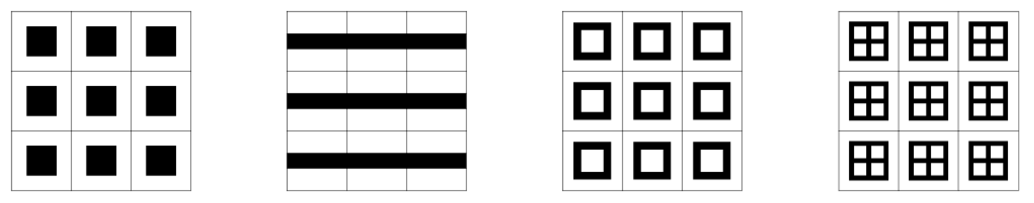
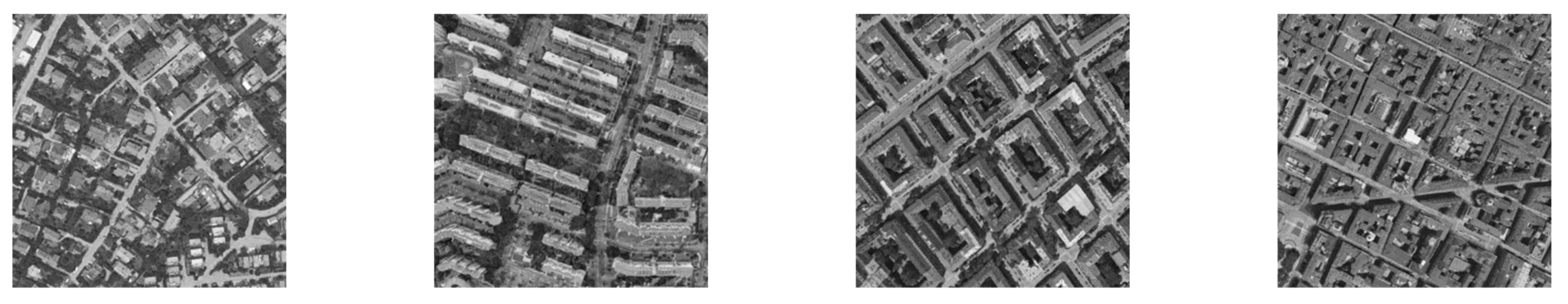
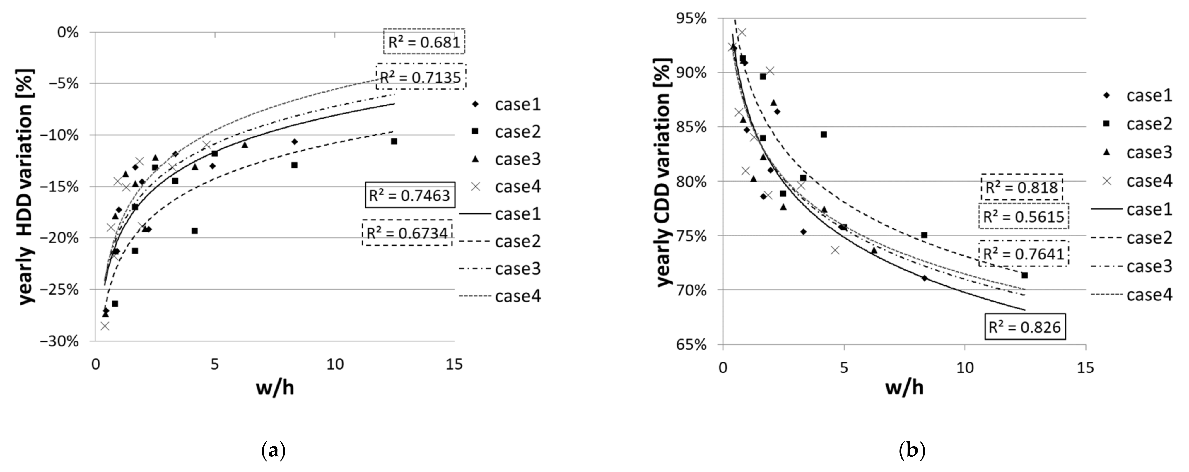
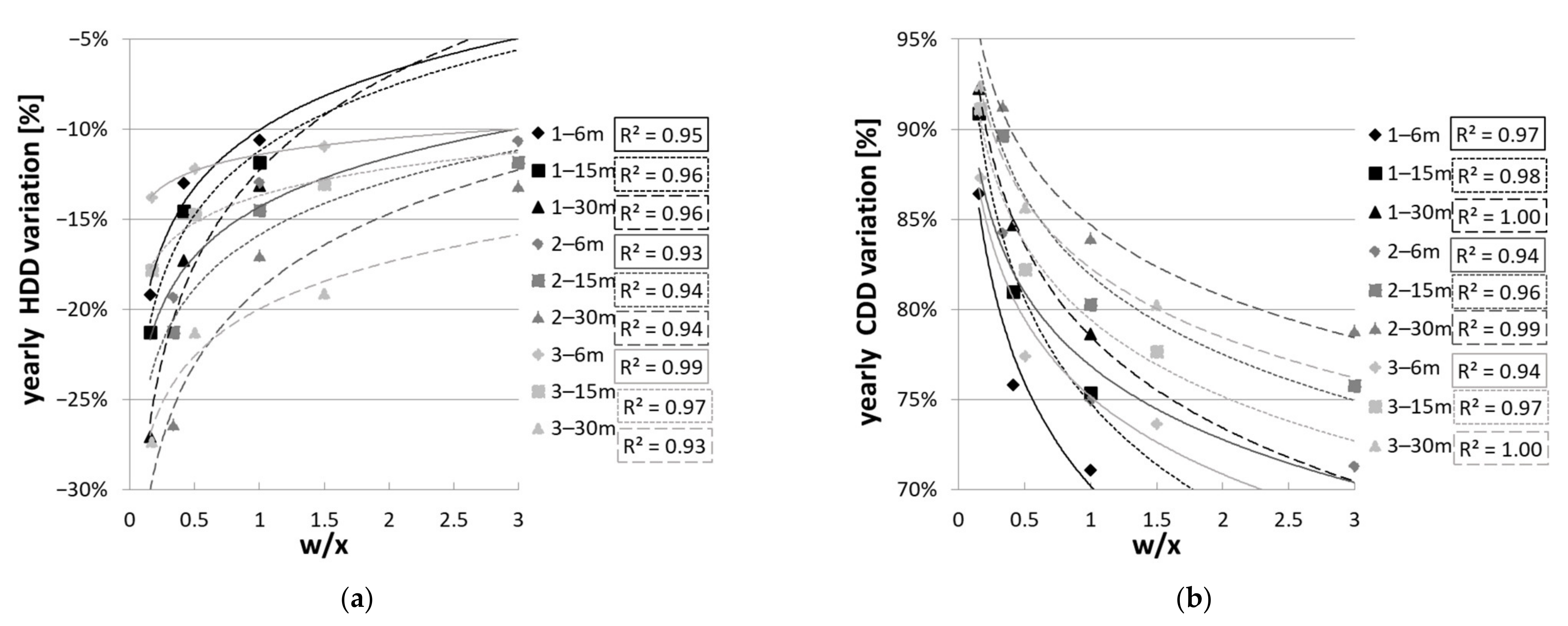
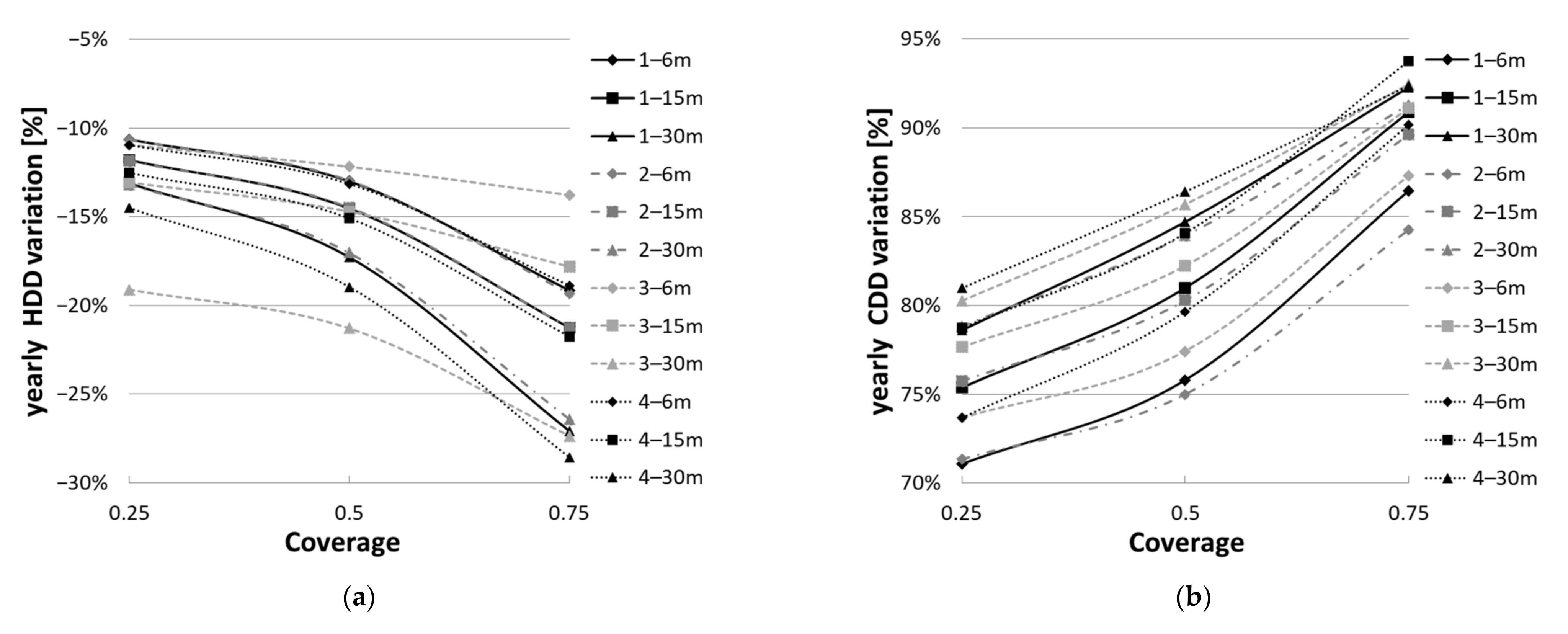
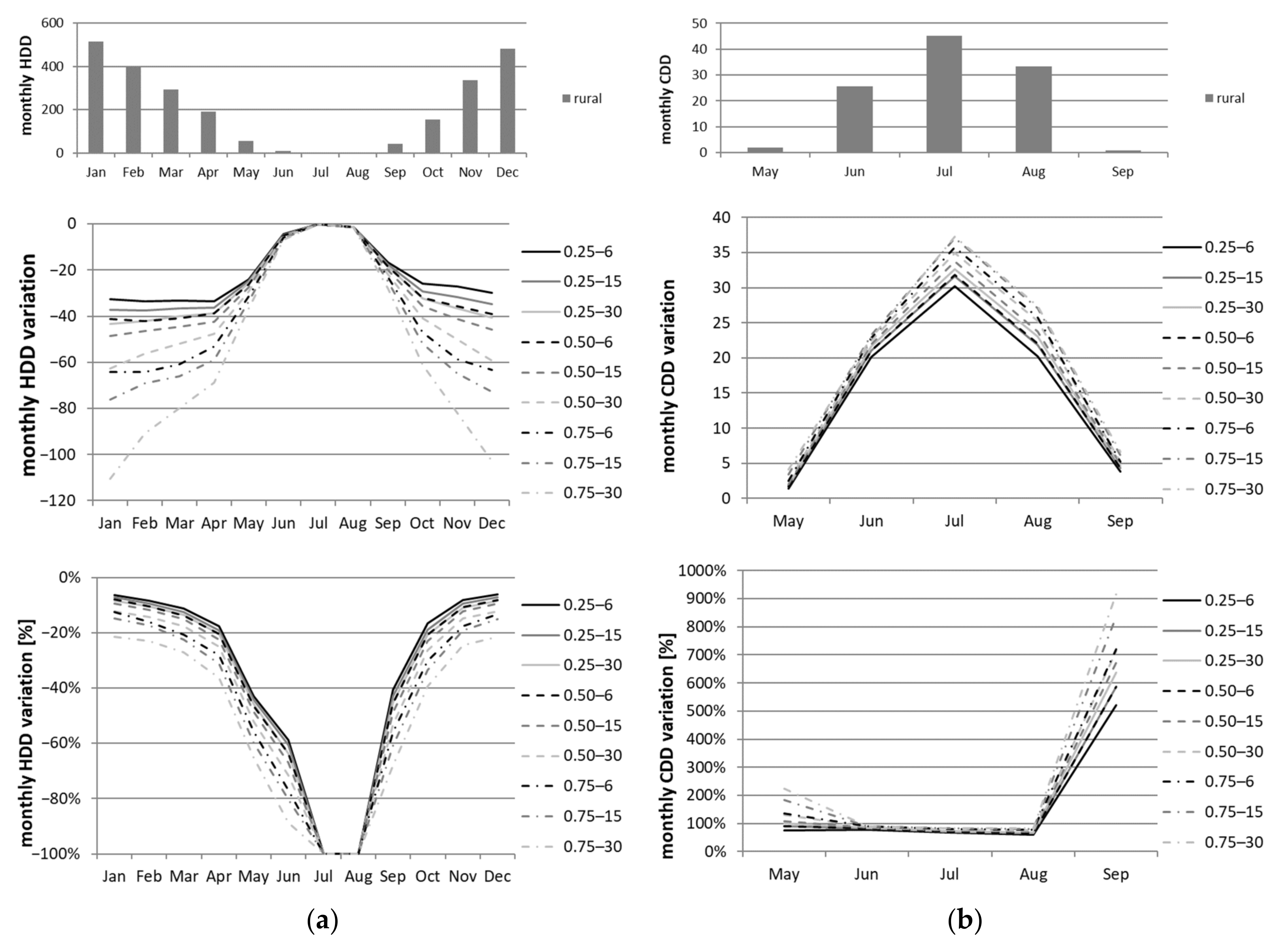
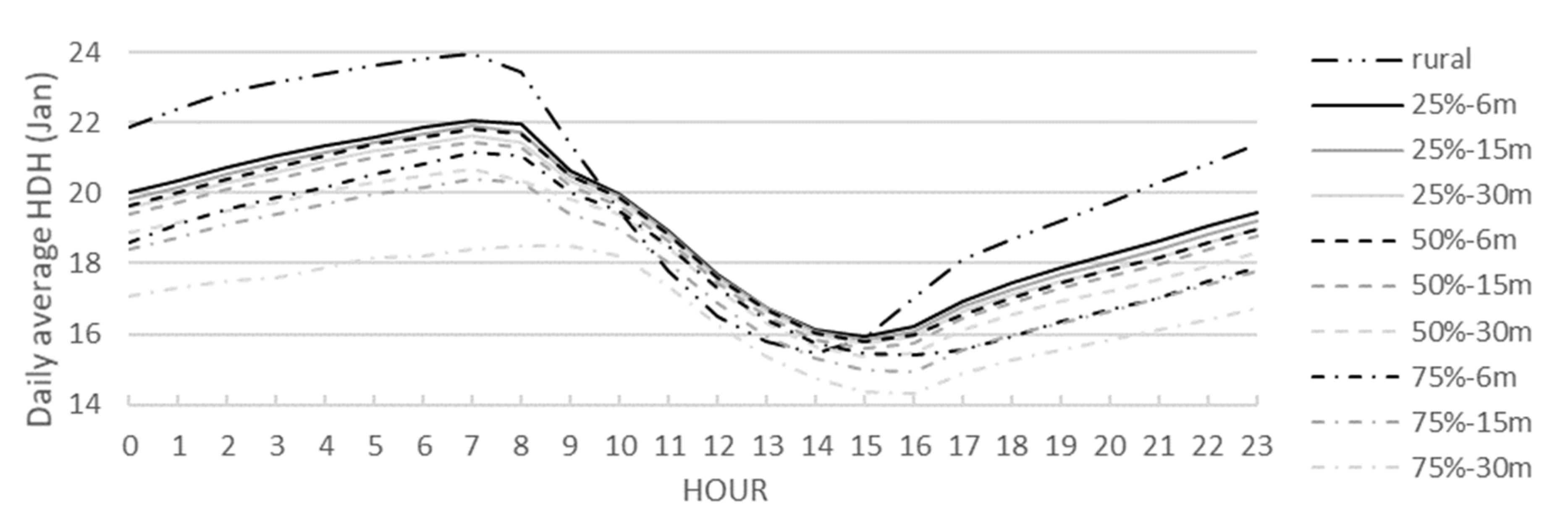
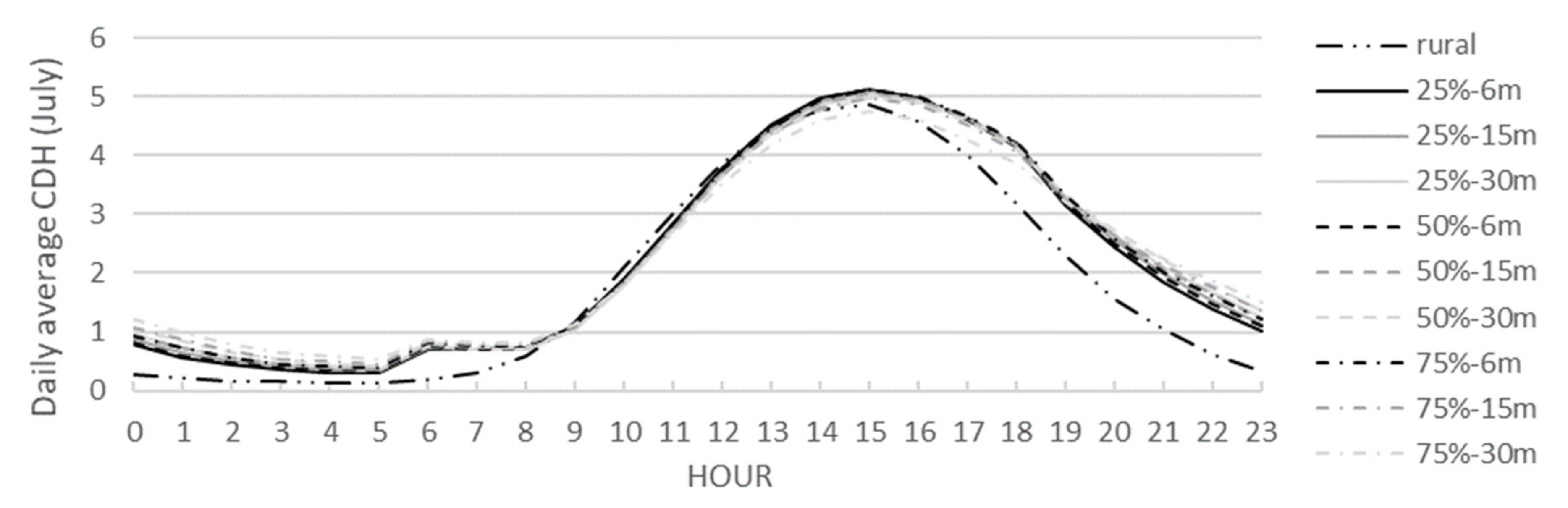
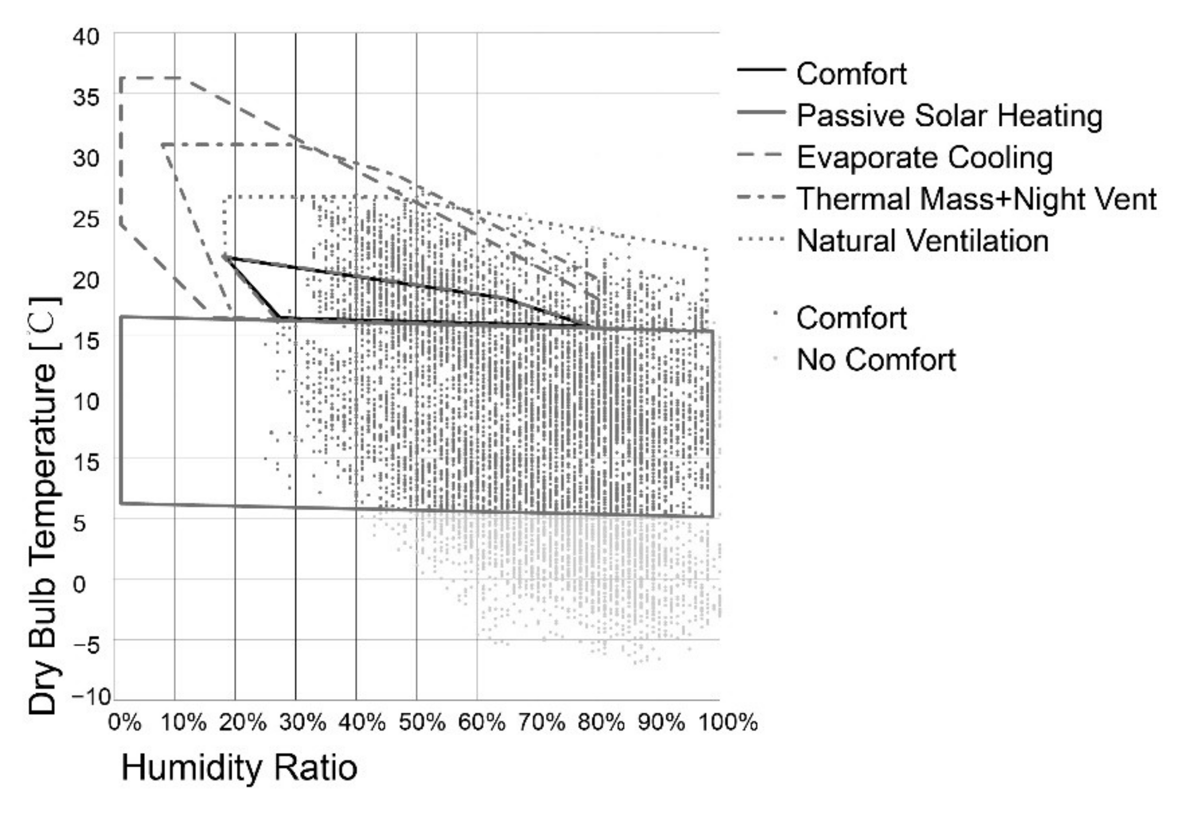
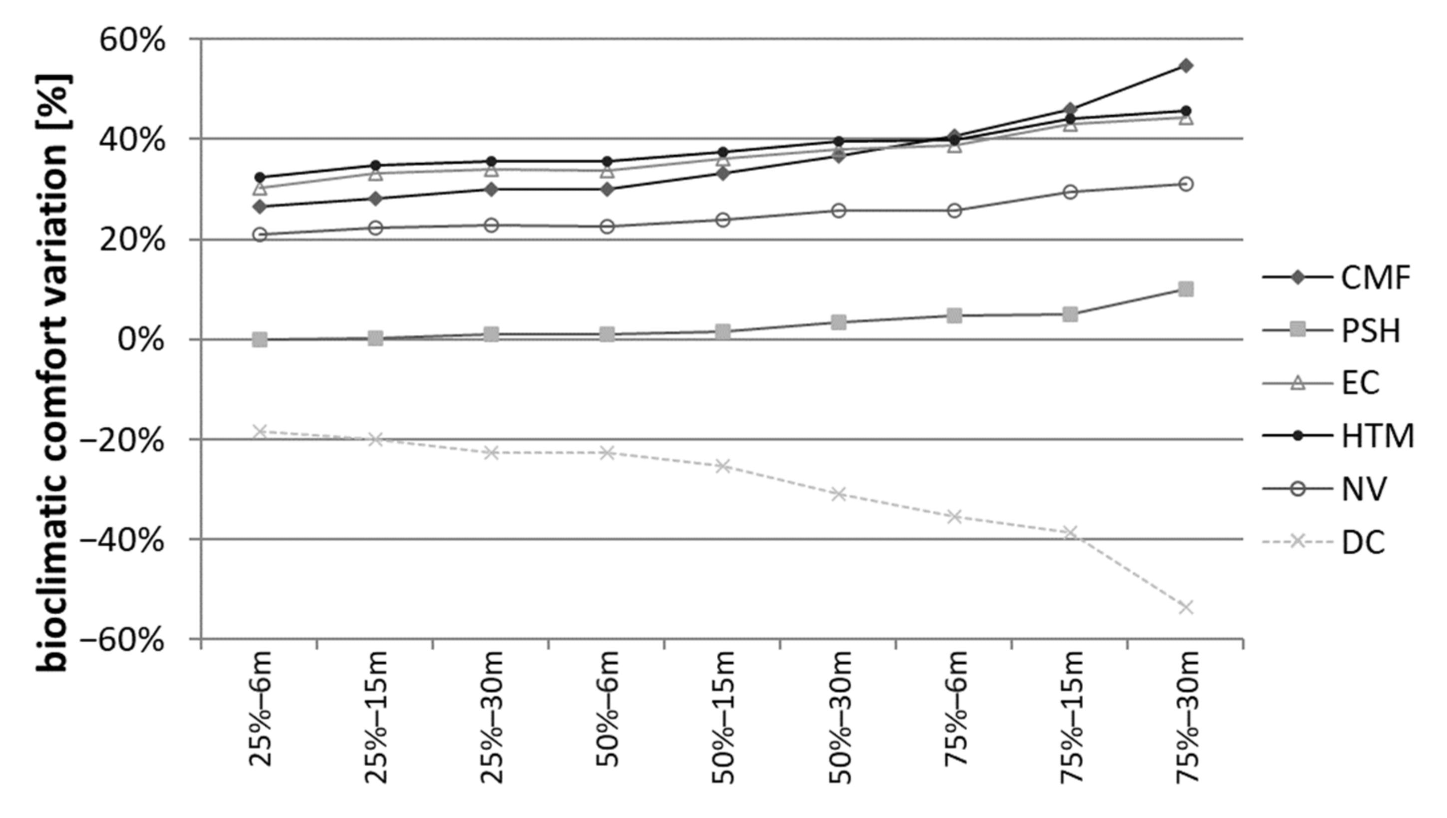
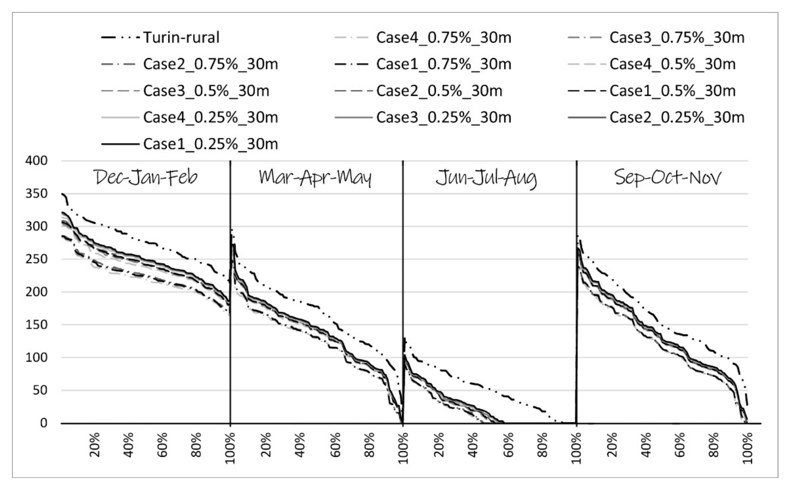
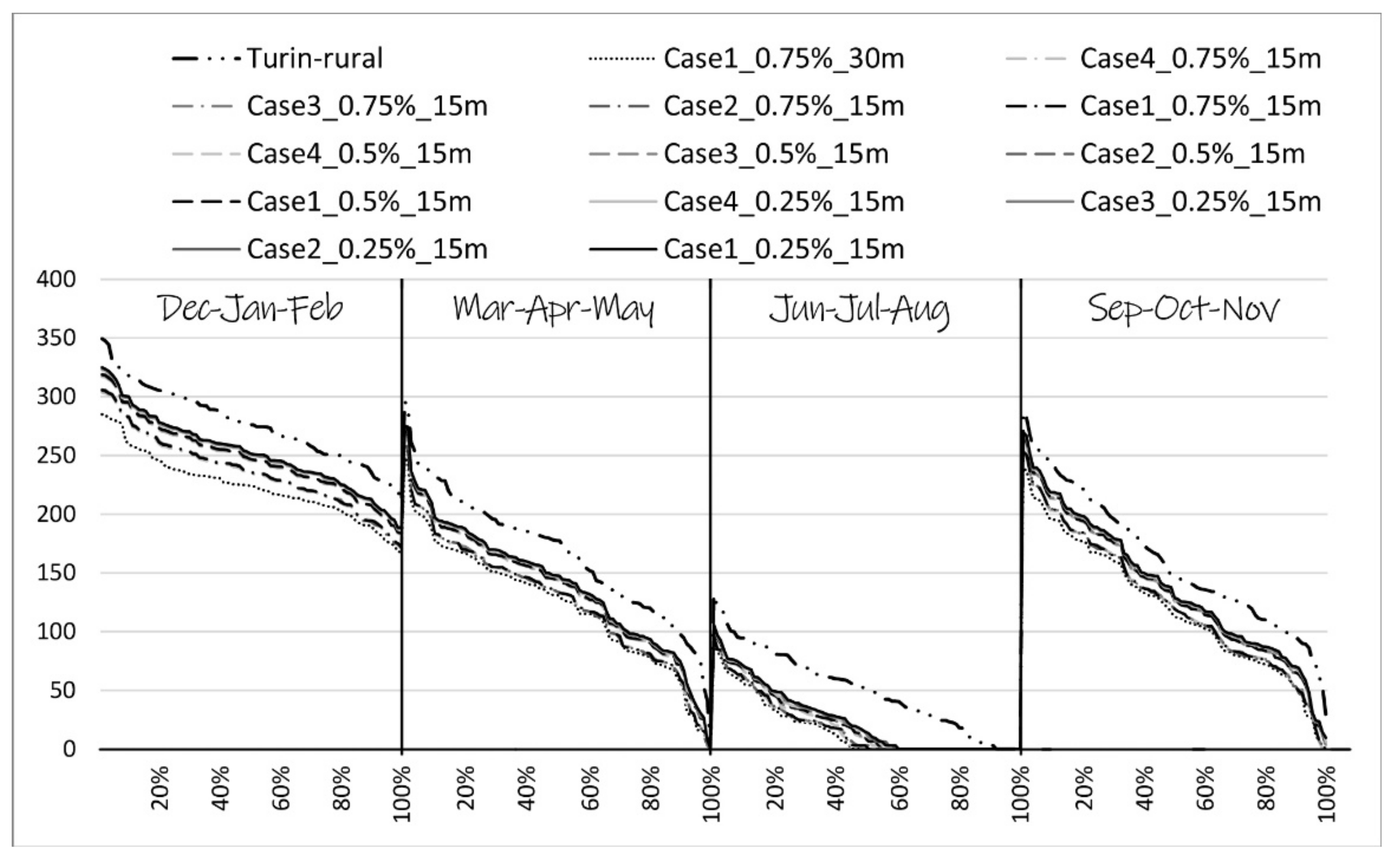
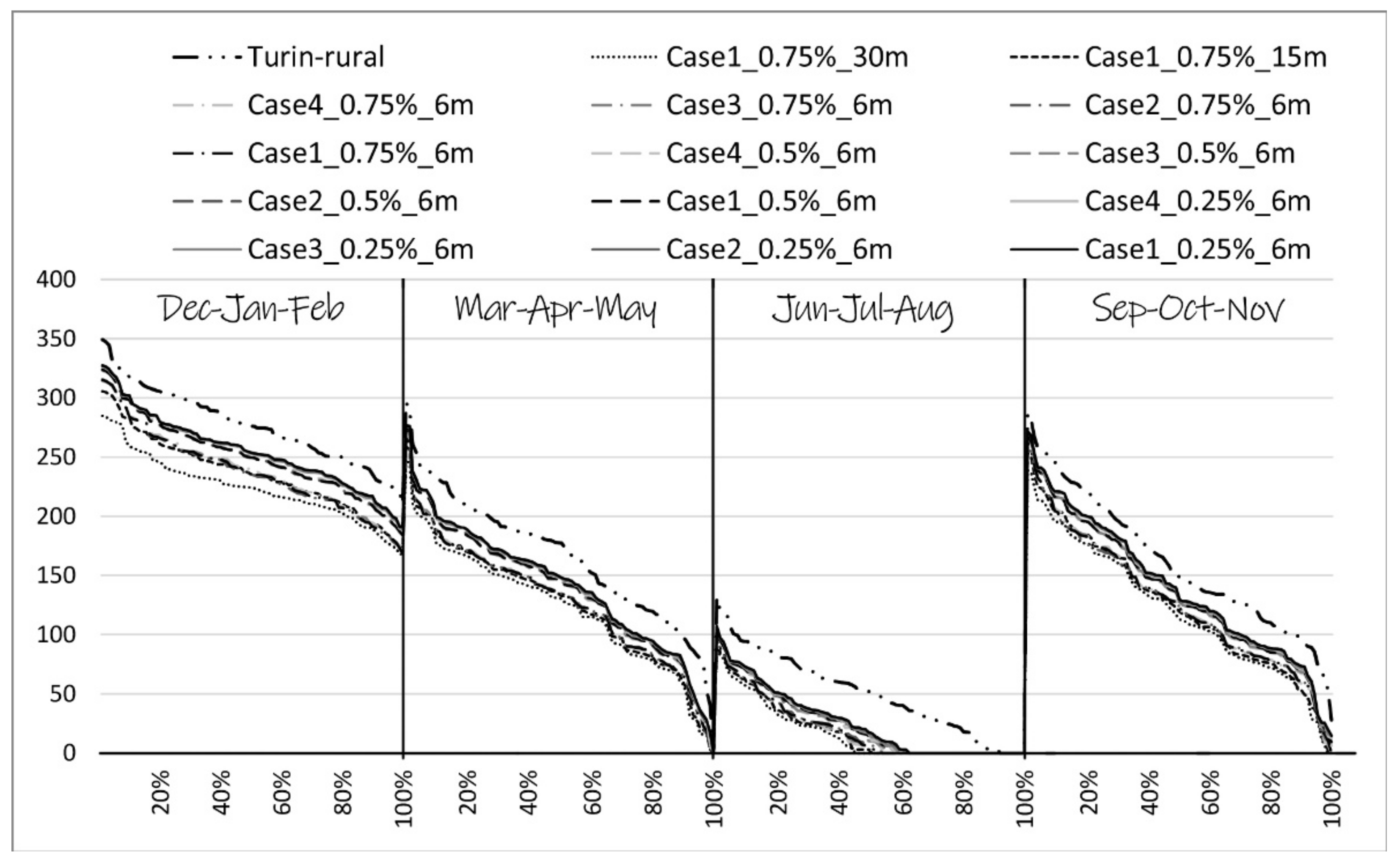
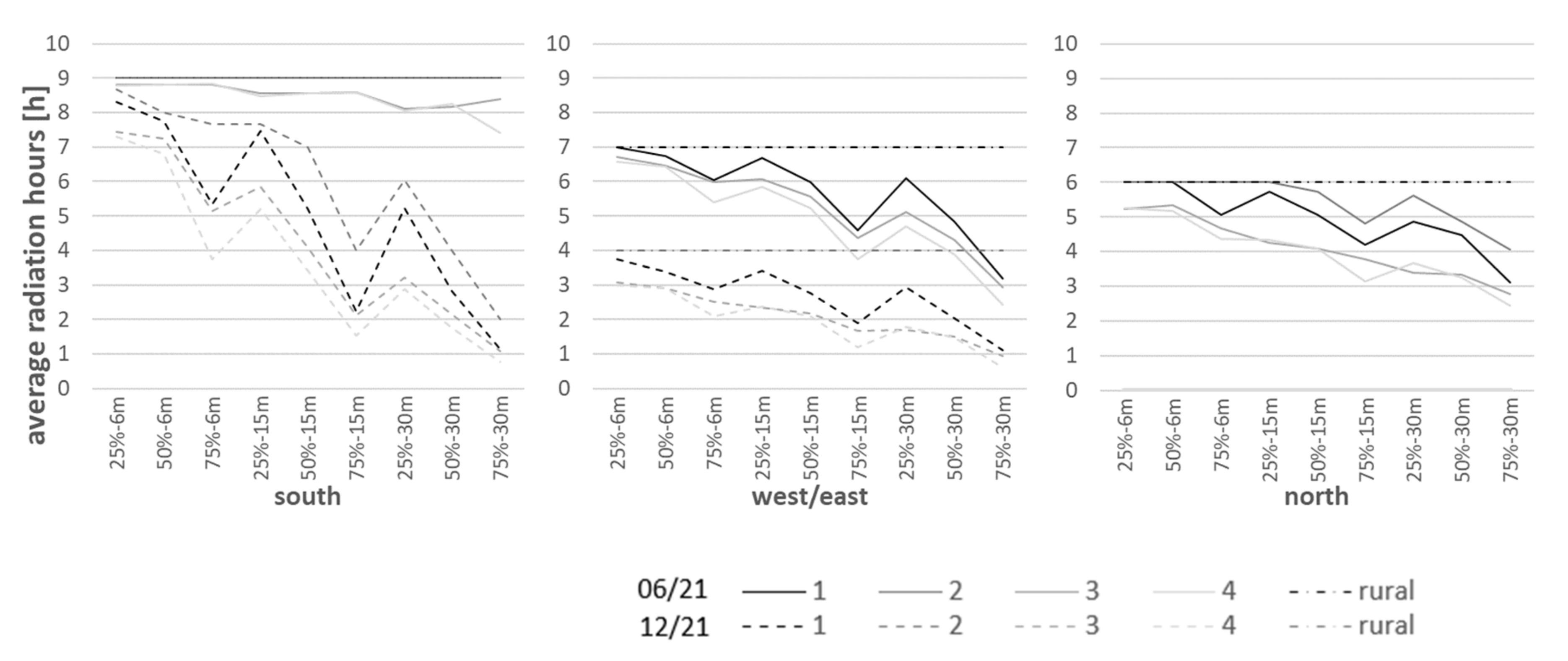
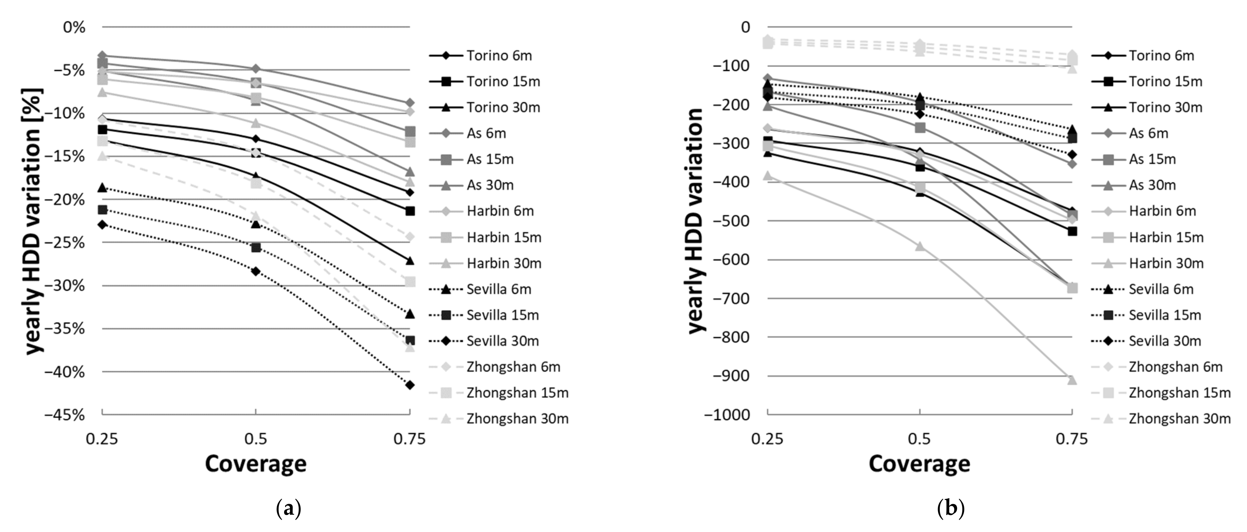
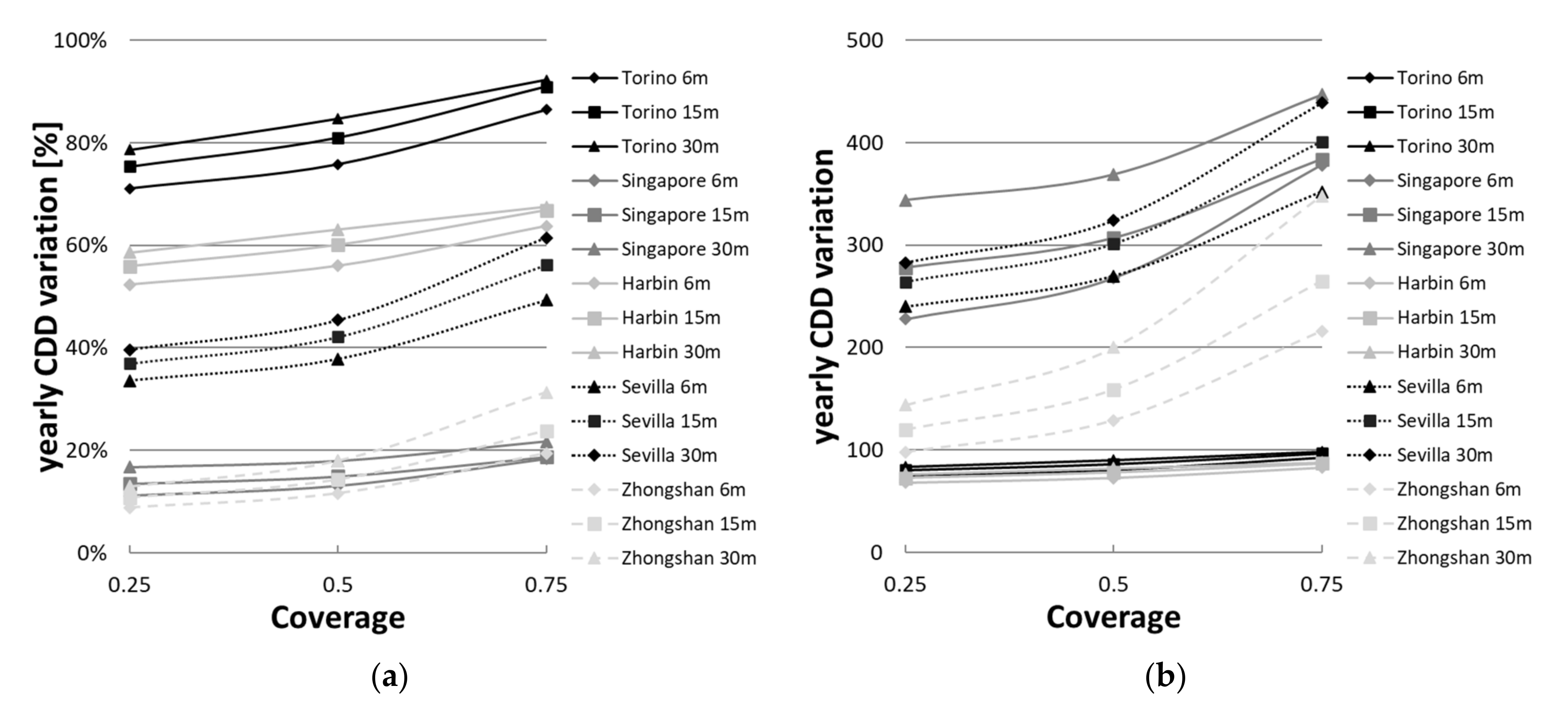
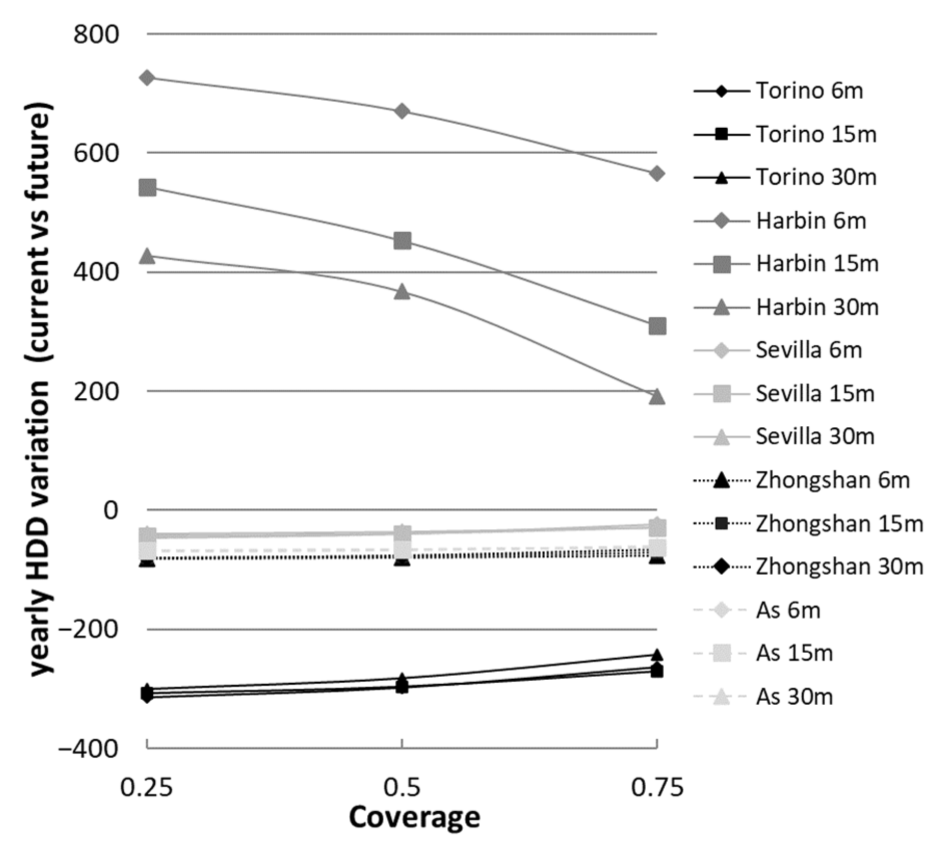
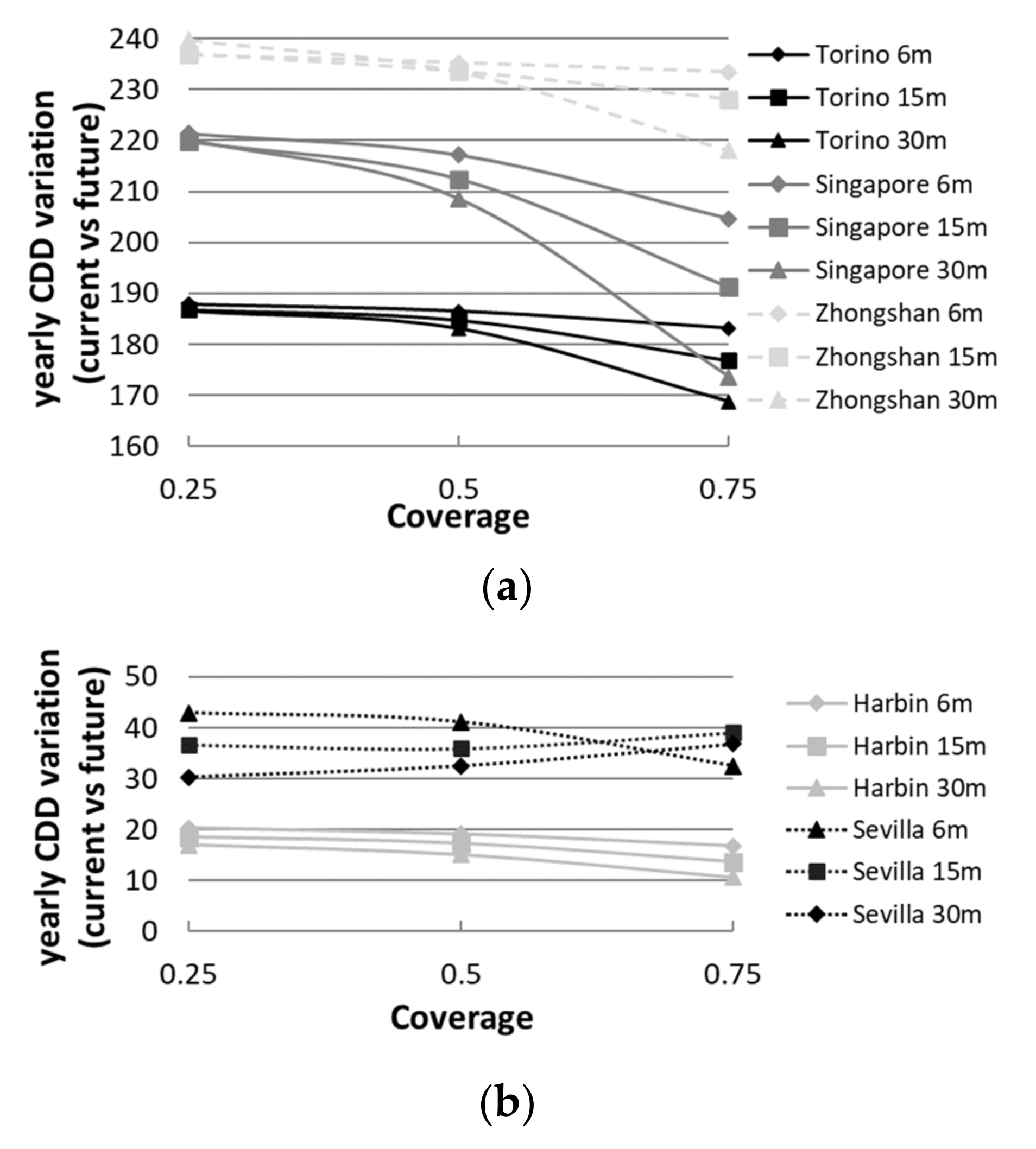
Table 1.
Morphological parameters for each urban morphological family.
| Morphological Type | Plot Top View | Coverage | Canyon w (m) 1 | Building Size X (m) | w/x | Building Height h (m) | w/h |
|---|---|---|---|---|---|---|---|
| Case 1 |  | 25% | 50 | 50 | 1 | 6 | 8.33 |
| 15 | 3.33 | ||||||
| 30 | 1.67 | ||||||
 | 50% | 29.3 | 70.7 | 0.41 | 6 | 4.88 | |
| 15 | 1.95 | ||||||
| 30 | 0.98 | ||||||
 | 75% | 13.4 | 86.6 | 0.15 | 6 | 2.33 | |
| 15 | 0.89 | ||||||
| 30 | 0.45 | ||||||
| Case 2 |  | 25% | 75 | 25 | 3 | 6 | 12.5 |
| 15 | 5 | ||||||
| 30 | 2.5 | ||||||
 | 50% | 50 | 50 | 1 | 6 | 8.33 | |
| 15 | 3.33 | ||||||
| 30 | 1.67 | ||||||
 | 75% | 25 | 75 | 0.33 | 6 | 4.17 | |
| 15 | 1.67 | ||||||
| 30 | 0.83 | ||||||
| Case 3 |  | 25% | 37.5 | 25 | 1.5 | 6 | 6.25 |
| 15 | 2.5 | ||||||
| 30 | 1.25 | ||||||
 | 50% | 25 | 50 | 0.5 | 6 | 4.17 | |
| 15 | 1.67 | ||||||
| 30 | 0.83 | ||||||
 | 75% | 12.5 | 75 | 0.17 | 6 | 2.08 | |
| 15 | 0.83 | ||||||
| 30 | 0.42 | ||||||
| Case 4 |  | 25% | 27.83 | / | / | 6 | 4.64 |
| 15 | 1.86 | ||||||
| 30 | 0.93 | ||||||
 | 50% | 19.32 | / | / | 6 | 3.22 | |
| 15 | 1.29 | ||||||
| 30 | 0.64 | ||||||
 | 75% | 11.61 | / | / | 6 | 1.94 | |
| 15 | 0.78 | ||||||
| 30 | 0.39 |
1 In case 3 and case 4, canyon width is the average value of canyon width and courtyard width.
Table 2.
Input and system parameters used in the performed UWG morphing processes.
| Category | UWG Input Parameter | Value | Unit |
|---|---|---|---|
| Pavement Parameters | Road Albedo | 0.1 | - |
| Pavement Thickness | 0.5 | m | |
| Thermal conductivity | 1 | W/(m⋅K) | |
| Volumetric heat capacity | 1,600,000 | J/m3K | |
| Vegetation Parameters | Veg Start Month | 3 | - |
| Veg End Month | 10 | - | |
| Vegetation Albedo | 0.25 | - | |
| Latent Fraction of Grass | 0.5 (winter) 0.3 (summer) | - | |
| Latent Fraction of Tree | 0.5 (winter) 0.7 (summer) | - | |
| Boundary-Layer | Urban Boundary Layer Height—Day | 1000 | m |
| Urban Boundary Layer Height—Night | 50 | m | |
| Inversion Height | 150 | m | |
| Circulation Coefficient | 1.2 | - | |
| UCM–UBL Exchange Coefficient | 0.3 | - | |
| Reference EPW Parameters | Rural average obstacle height | 0.1 | m |
| Rural road vegetation coverage | 0.9 | - | |
| RSM temperature reference height | 2.6 | m | |
| RSM wind reference height | 10 | m |
UWG: Urban weather generator.
Table 3.
Hours of comfort and passive building strategies of comfort in rural Turin. CMF: Comfort; PSH: Passive Solar Heating; EC: Evaporative Cooling; HTM: Thermal Mass + Night Vent; NV: Natural Ventilation; DC: Discomfort in all strategies.
Table 3.
Hours of comfort and passive building strategies of comfort in rural Turin. CMF: Comfort; PSH: Passive Solar Heating; EC: Evaporative Cooling; HTM: Thermal Mass + Night Vent; NV: Natural Ventilation; DC: Discomfort in all strategies.
| CMF | PSH | EC | HTM | NV | DC | |
|---|---|---|---|---|---|---|
| hours (h) | 599 | 4897 | 785 | 832 | 1107 | 2155 |
| percentage (%) | 6.84 | 55.90 | 8.96 | 9.53 | 12.64 | 24.60 |
Table 4.
Comparison between four selected urban tissues and morphological building types.
| Arial Image of the Selected Urban Tissue | Axonometric Representation of the Real Urban Tissue | Axonometric Representation of Morphological Types | Morphological Data |
|---|---|---|---|
 |  |  | Case 1: Oslo suburban area Avg. building height: 7.7 m Coverage: 20% |
 |  |  | Case 2: Singapore Ang Mo Kio residential area Avg. building height: 38 m Coverage: 21% |
 |  |  | Case 3: Oslo downtown area Avg. building height: 18.4 m Coverage: 37% |
 |  |  | Case 4: Torino historical city center Avg. building height: 18.2 m Coverage: 0.63% |
Table 5.
MSE: Mean squared error; RMSE: Root mean squared error; MAE: Mean absolute error; MAE: Mean absolute percentage error. R2 between the UWG results of the hourly air temperature of selected urban issues and morphological building types.
Table 5.
MSE: Mean squared error; RMSE: Root mean squared error; MAE: Mean absolute error; MAE: Mean absolute percentage error. R2 between the UWG results of the hourly air temperature of selected urban issues and morphological building types.
| Morphological Type | MSE | RMSE | MAE | MAPE | R2 |
|---|---|---|---|---|---|
| Case 1 | 0.0002 | 0.0147 | 0.0021 | 0.00% | 1.0000 |
| Case 2 | 0.0028 | 0.0528 | 0.0278 | 0.02% | 0.9994 |
| Case 3 | 0.0100 | 0.100 | 0.0692 | 0.53% | 0.9999 |
| Case 4 | 0.1671 | 0.4088 | 0.2367 | 4.18% | 0.9984 |
Table 6.
Comparison of yearly HDD in current and future-scenario conditions in six climates—rural cases.
Table 6.
Comparison of yearly HDD in current and future-scenario conditions in six climates—rural cases.
| Torino | Singapore | Harbin | Sevilla | Zhongshan | Ås | |
|---|---|---|---|---|---|---|
| current | 2469.49 | 0.00 | 5061.61 | 790.75 | 288.41 | 4006.80 |
| future | 2089.44 | 0.00 | 5182.16 | 699.34 | 213.71 | 3940.21 |
| variation | −380.05 | / | 120.55 | −91.41 | −74.70 | −66.59 |
| % | −15% | / | 2% | −12% | −26% | −2% |
Table 7.
Comparison of yearly CDD in current and future-scenario conditions in six climates—rural cases.
Table 7.
Comparison of yearly CDD in current and future-scenario conditions in six climates—rural cases.
| Torino | Singapore | Harbin | Sevilla | Zhongshan | Ås | |
|---|---|---|---|---|---|---|
| current | 106.61 | 2056.22 | 130.15 | 714.47 | 1111.81 | 0.94 |
| future | 257.31 | 2269.32 | 158.74 | 826.02 | 1314.54 | 3.07 |
| variation | 150.70 | 213.11 | 28.58 | 111.56 | 202.73 | 2.13 |
| % | 141% | 10% | 22% | 16% | 18% | 226% |
Publisher’s Note: MDPI stays neutral with regard to jurisdictional claims in published maps and institutional affiliations. |
© 2021 by the authors. Licensee MDPI, Basel, Switzerland. This article is an open access article distributed under the terms and conditions of the Creative Commons Attribution (CC BY) license (https://creativecommons.org/licenses/by/4.0/).
Share and Cite
MDPI and ACS Style
Chiesa, G.; Li, Y. Including Urban Heat Island in Bioclimatic Early-Design Phases: A Simplified Methodology and Sample Applications. Sustainability 2021, 13, 5918. https://0-doi-org.brum.beds.ac.uk/10.3390/su13115918
AMA Style
Chiesa G, Li Y. Including Urban Heat Island in Bioclimatic Early-Design Phases: A Simplified Methodology and Sample Applications. Sustainability. 2021; 13(11):5918. https://0-doi-org.brum.beds.ac.uk/10.3390/su13115918
Chicago/Turabian StyleChiesa, Giacomo, and Yingyue Li. 2021. "Including Urban Heat Island in Bioclimatic Early-Design Phases: A Simplified Methodology and Sample Applications" Sustainability 13, no. 11: 5918. https://0-doi-org.brum.beds.ac.uk/10.3390/su13115918
Note that from the first issue of 2016, this journal uses article numbers instead of page numbers. See further details here.