4.2. Results from GM (1,1)
Table 2 and
Table 3 compare the unemployment rate in rural and urban areas of Vietnam’s six administrative regions from 2014 to 2025. It is quite evident that the unemployment rate for urban areas would follow a downward trend until 2025 due to the industrialization and modernization process. By contrast, the rural unemployment rate might continue to rise because of the process’s impacts. It could be seen that the unemployment rate in the urban areas tends to be higher as opposed to that in rural areas. Specifically, the average forecasted unemployment rate in urban regions ranges between 2.5% and 3.5%, while the figures for rural areas are below 2%. The reason for this phenomenon is not explained by the population scale of each region since, according to Vietnam General Statistics Office, there were approximately 37,6 million rural laborers and about 18 million in urban regions as of 2019 (
https://www.gso.gov.vn/ accessed on 30 July 2020). Because the population scale could not explain the higher unemployment rate in urban regions, Vietnamese experts have interpreted a rising demand for qualified laborers in big cities; with this demand comes stricter recruitment procedures and lower the chances for unqualified laborers.
Moreover, high-skilled laborers look for jobs that offer decent pay, and low-skilled workers do everything for their livelihood. Therefore, high-skilled laborers might suffer from frictional unemployment during the job-seeking period. In addition, reference data from the GSO indicated a downward trend for the RRD because the region now has the highest education level in Vietnam. In 2018, the proportions of secondary school, high school, and university graduates were estimated at 39% and 31.6%, respectively. Moreover, supporting the trend is an influx of Foreign Direct Investment (FDI) into the region. According to statistics from the Foreign Direct Investment Department of the Ministry of Planning and Investment, as of 2015, the number of newly registered investment projects was recorded at 606, amounting to USD 2.6 billion. In addition to that, capital-increasing projects accounted for about 62.5% of the region’s total FDI.
Moreover, the accumulated calculations specified the number of 5800 registered projects since the ‘Doi Moi’ policy; foreign investment projects in the Red River Delta made up 30% of the total projects in Vietnam, accounting for approximately 26% of the total amount of FDI in the country. The FDI data from a report in 2017 by the Foreign Direct Investment Department showed a significant increase in the number of new projects. It was estimated that in 2017, the Red River Delta had attracted nearly 7202 projects, which were worth USD 81.76 billion. According to GM (1,1) model, the average forecastings of unemployment rates in urban and rural areas are shown in
Figure 1.
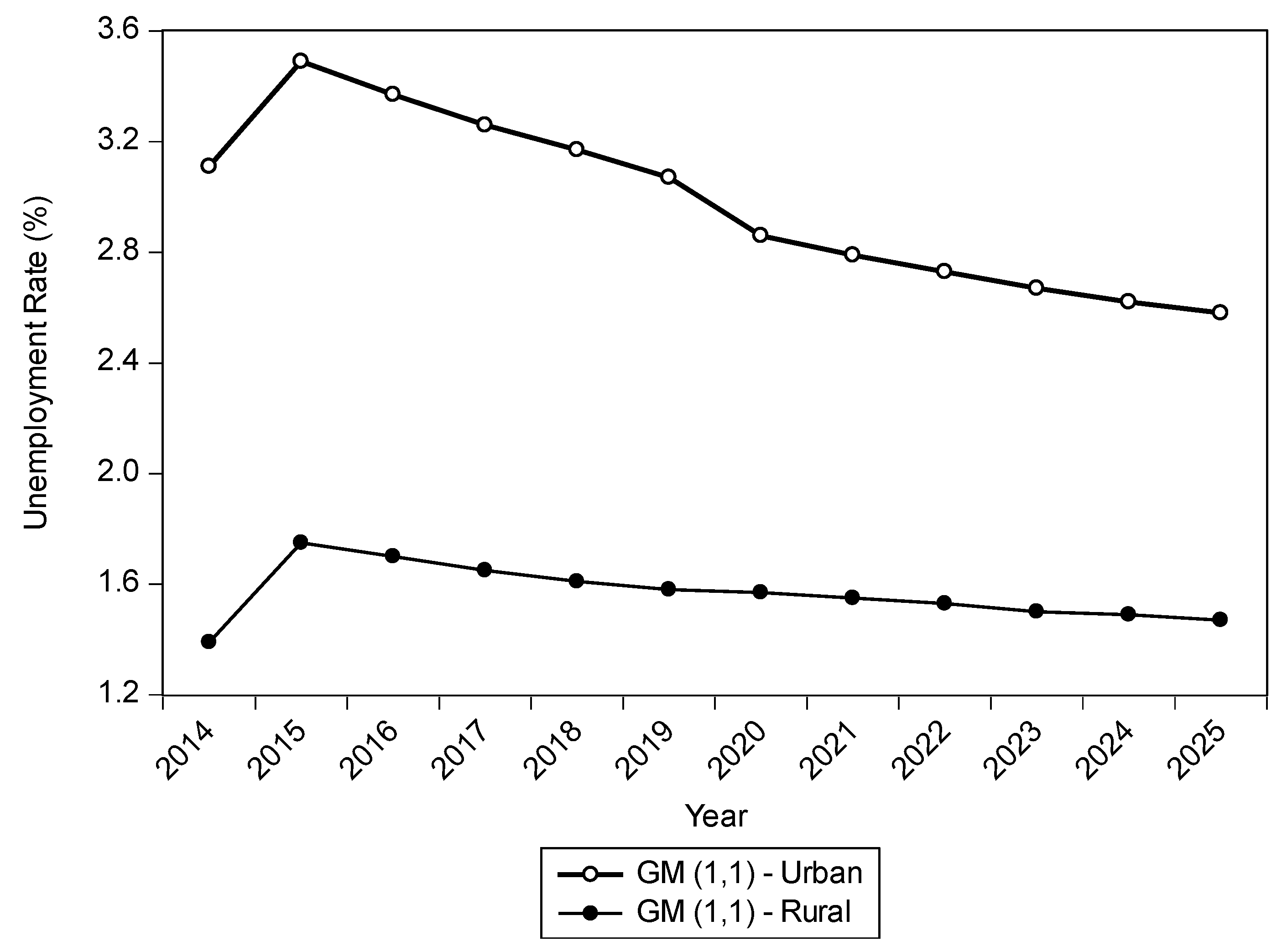
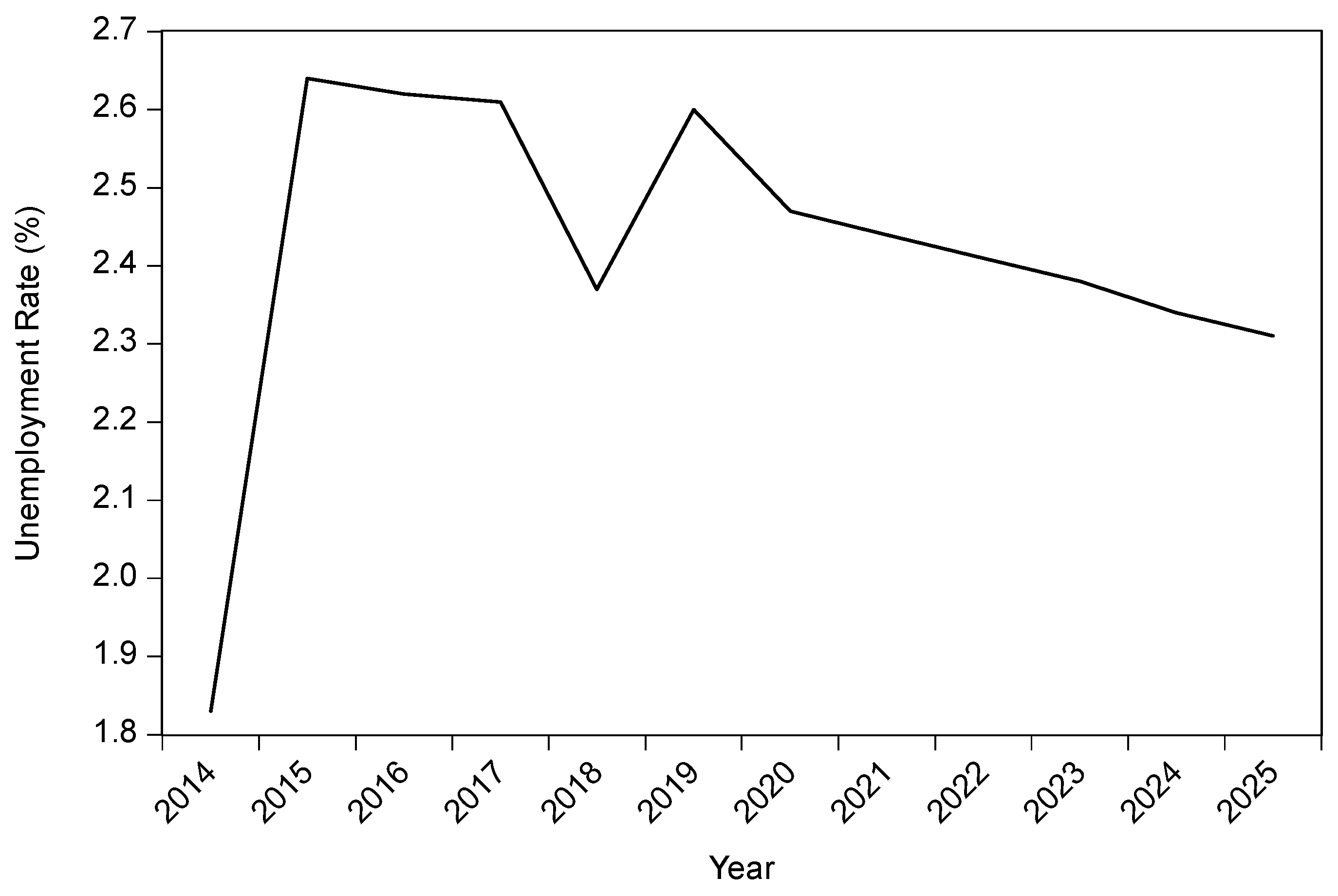
From
Figure 1, it is seen that the forecasts of unemployment rates show a descending trend based on GM (1,1) model. Average forecasting of urban areas’ unemployment rates will reach above 2.5%. However, this rate decreases by approximately 1.5% in rural areas. In the context of GM (1,1) model predictions, the unemployment rates for each region will be evaluated between
Figure 2,
Figure 3,
Figure 4,
Figure 5,
Figure 6,
Figure 7,
Figure 8,
Figure 9,
Figure 10,
Figure 11,
Figure 12 and
Figure 13, separately.
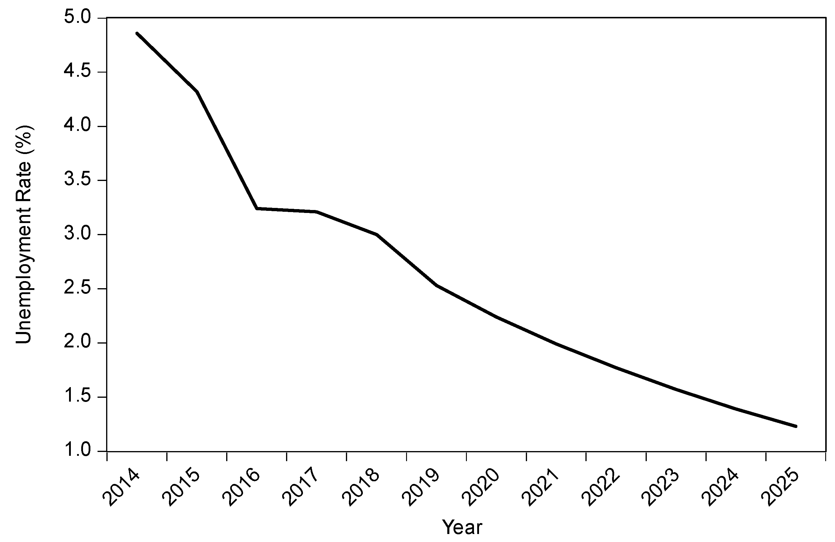
According to
Figure 2, it is clear that the unemployment rate in the urban area of the Red River Delta region declined as time went on. The unemployment rate in that region was around 4.86%; then it decreased by 11.1% to 4.32% in the next year. After that, the unemployment rate declined significantly by 25% to around 3.24% in 2016. Since the sharp decline in 2016, in the following years, the unemployment rate maintained at around 3% in 2018. In the latest update, the unemployment rate in the region decreased to 2.53% in 2019. In addition, it is estimated that the Red River Delta’s urban area’s unemployment rate would continue to decrease in the following years, from 2.53% to 1.23% in 2025.
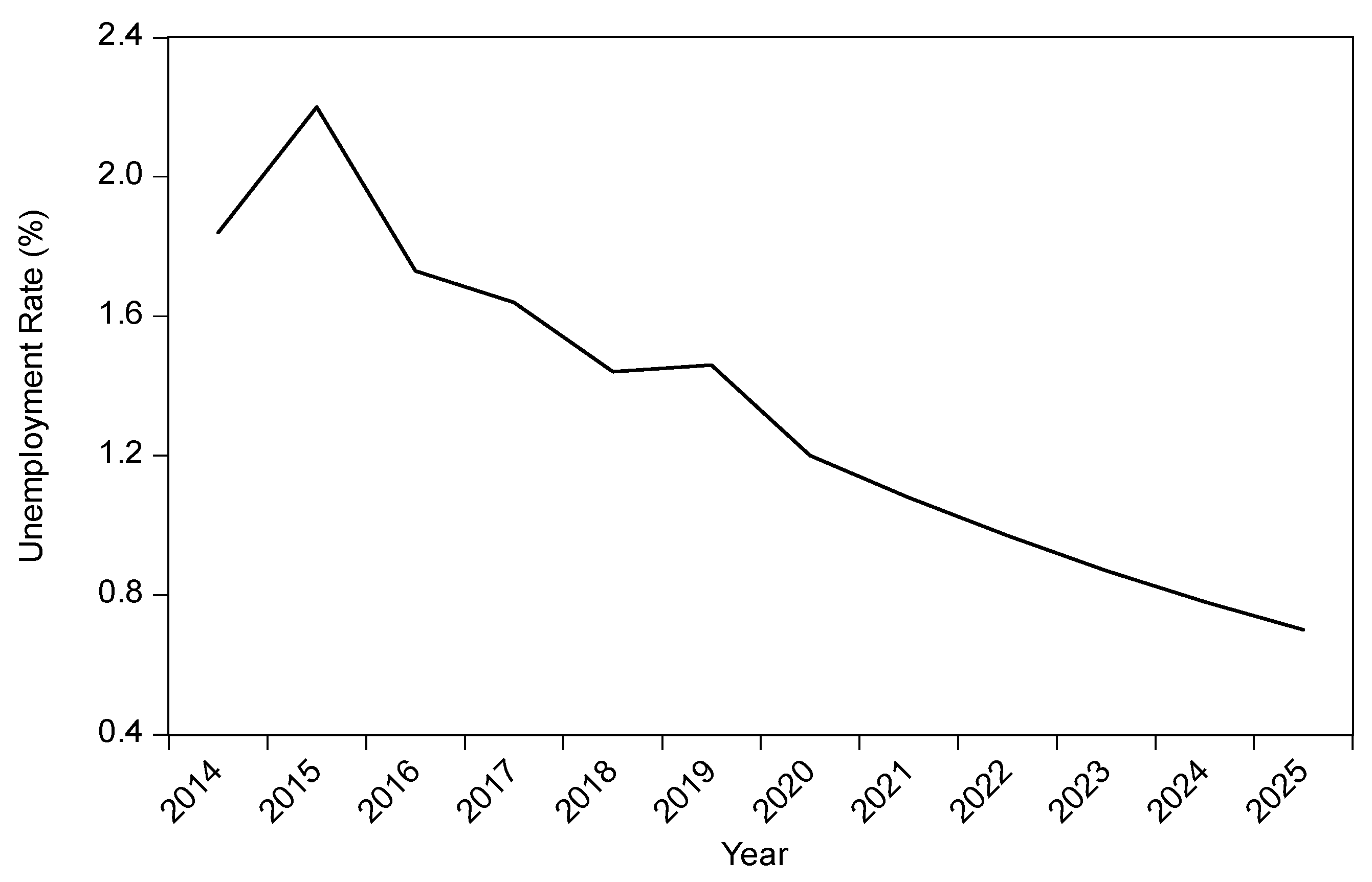
Regarding the unemployment rate in the Red River Delta’s rural area, as shown in
Figure 3, the unemployment rate decreased for most of the period. On the one hand, there was only a sharp increase in the year 2015. In 2014, the number of unemployed in the total number of employed people was recorded at 1.84%. In 2015, the unemployment rate increased by approximately 20% to 2.2%, which declined by 21.4% to 1.73% in 2016. In the next three years, the unemployment rates were between 1.44% and 1.64%; it could continue this downward trend and decrease to 0.7% by 2025.
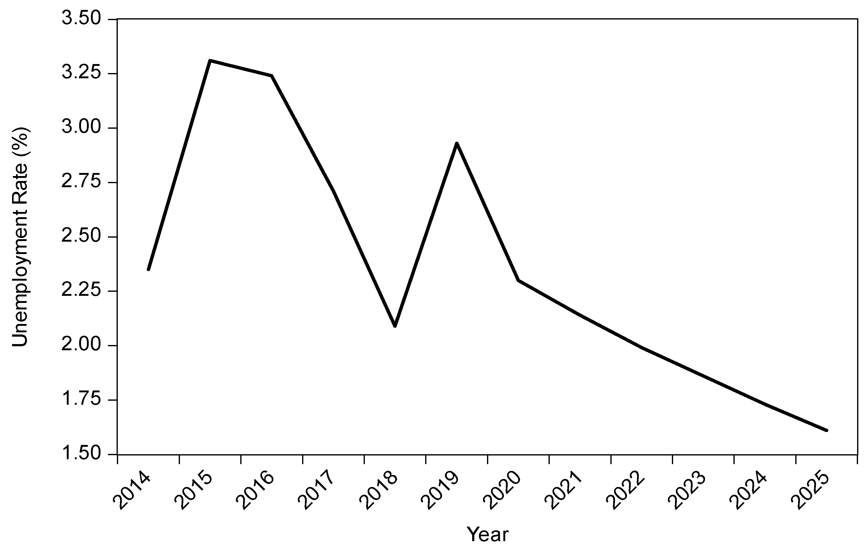
As shown in
Figure 4, the urban unemployment rate in the Northern Midlands and Mountains was estimated at 2.4% in 2014. It then rose by 37.5% to 3.3% in 2015. However, the unemployment rate declined significantly to 2.09% in 2018, which was 22% lower than the rate for the year 2016. The year 2019 saw an increasing unemployment rate at 2.93%, up 38% from the previous year. In the next six years, the unemployment rate is estimated to continue a downward trend as it would decrease gradually from 2.9% to 1.6% in 2025.
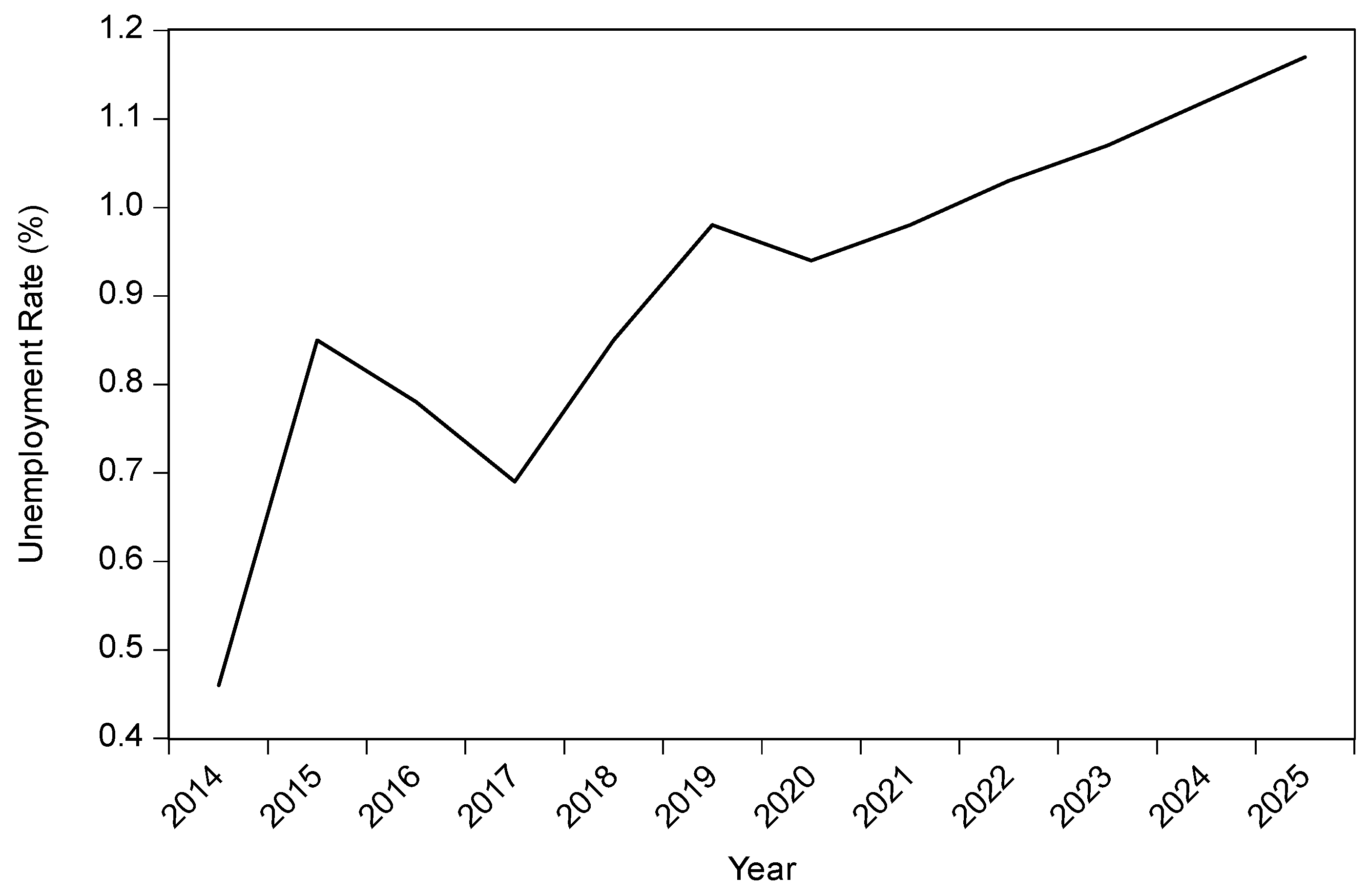
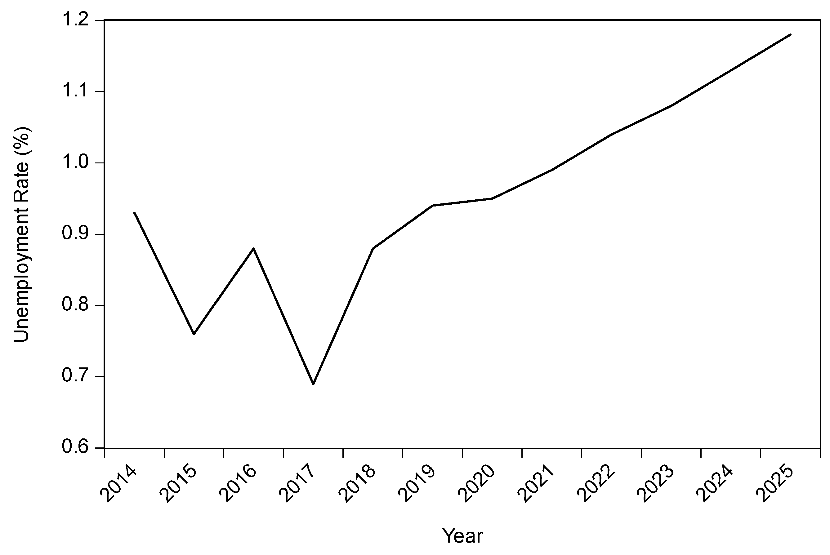
Figure 5 shows the unemployment rate for the rural area of the Northern Midlands and Mountains. It can be seen that the rural unemployment rate reached 0.85% in 2015, a tremendous increase from 2014, then it decreased to 0.78% in 2016. Following the downward trend, the rate decreased to 0.69% in 2017. There were increases in the rate of 0.85% in 2018 and 0.98% in 2019. Estimations for the period from 2020–2025 indicate that the unemployment rate would continue its downward trend as it could increase to about 1.17% by 2025.
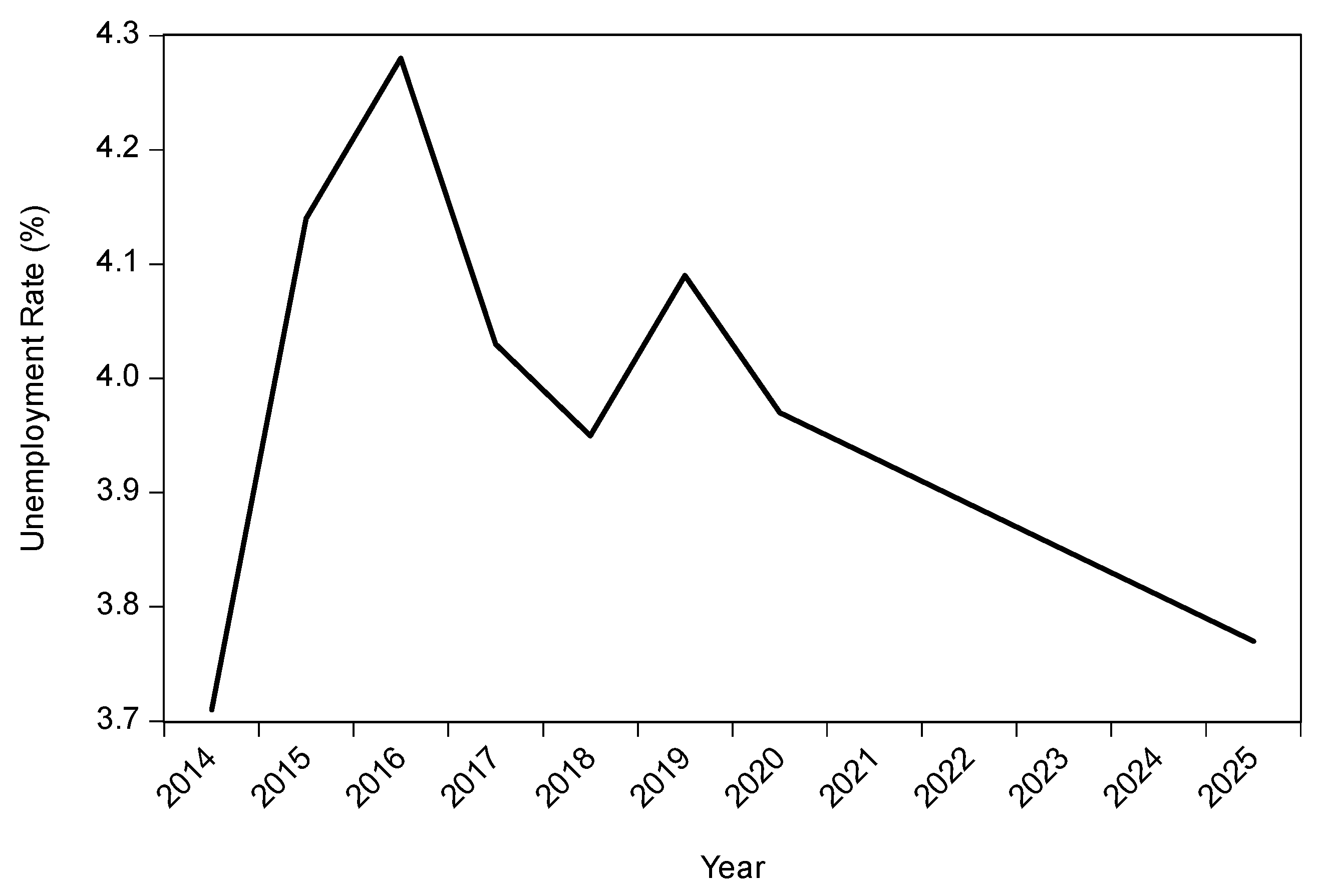
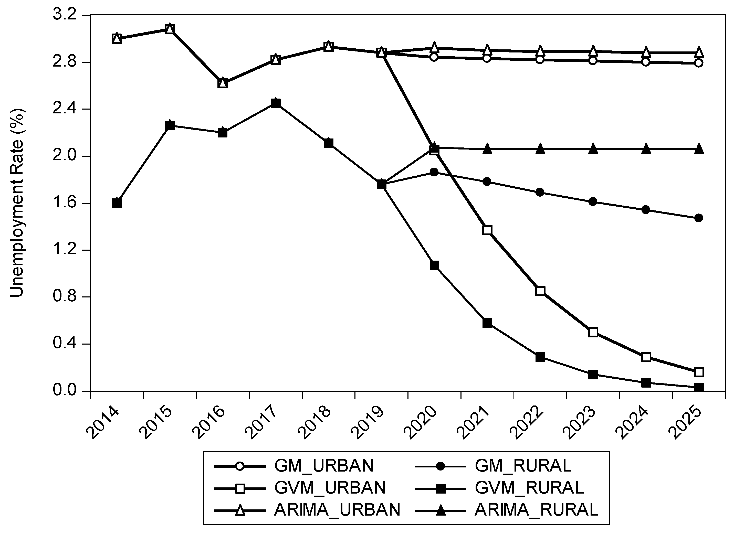
Figure 6 shows the unemployment rate for the urban area of the North Central region. The North Central region’s unemployment rate was quite volatile. Starting at 3.71% in 2014, it increased at the rate of 11.6% to 4.14% in 2015. In the following years, the urban unemployment rate fluctuated between 3.95% to 4.28%. The rate is then expected to decrease for the next six consecutive years to around 3.77% in 2025.
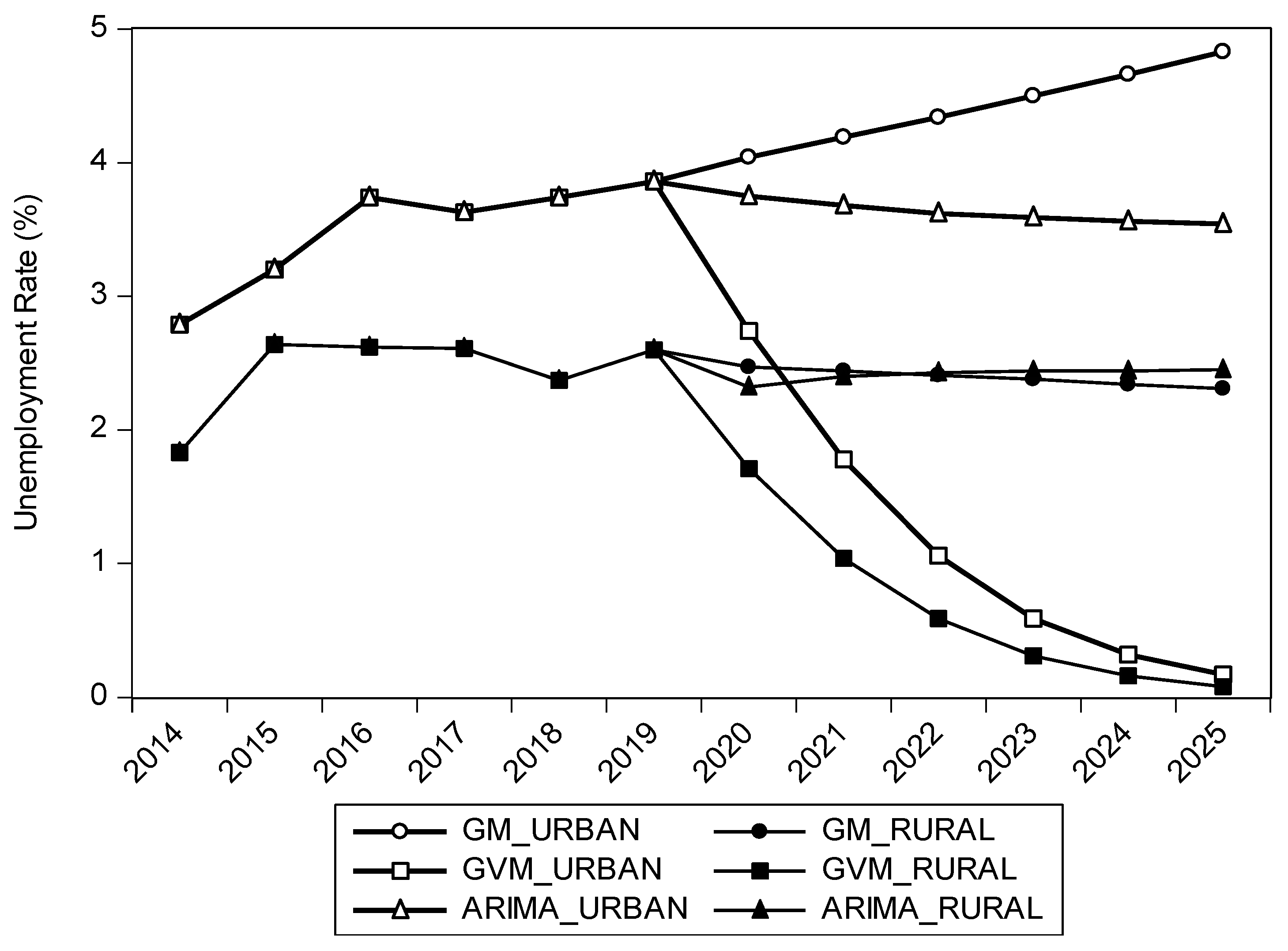
According to
Figure 7, the unemployment rate increased continuously from around 12% to 14% in the first three years of the period. Nevertheless, it fluctuated around 2% in the next three years, and this trend is estimated to continue until 2025.
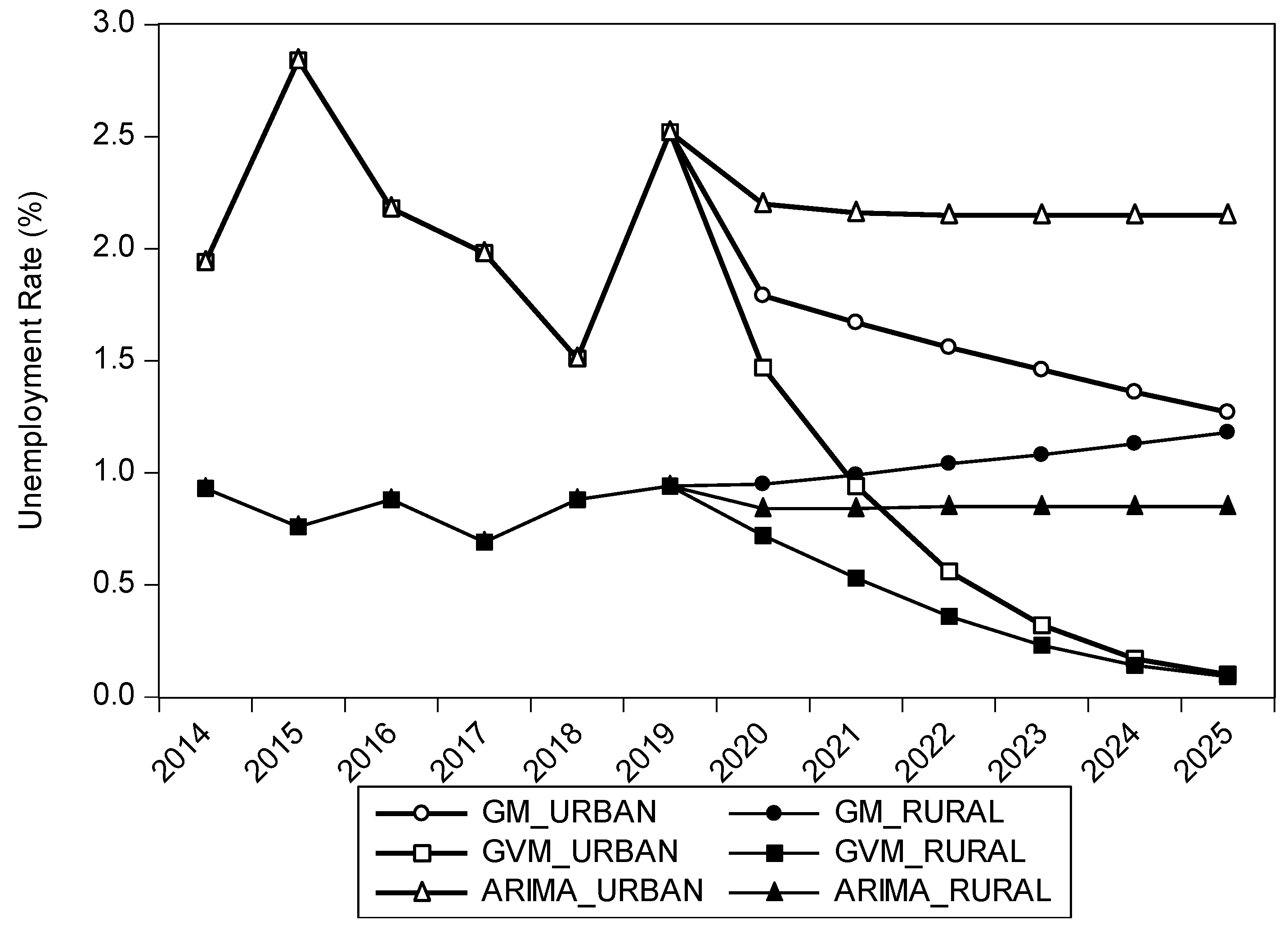
Concerning the percentage of the unemployed in the Highlands region’s urban area, it is pretty visible that the rate increased by nearly 50% from 1.94% in 2014 to 2.84% in 2015 (see
Figure 8). After that, the rate experienced declines in 2016, 2017, and 2018 before witnessing a high rise in 2019. It is expected that the rate could continue its downward trend in the next six years as it might decrease to 1.27% in 2025.
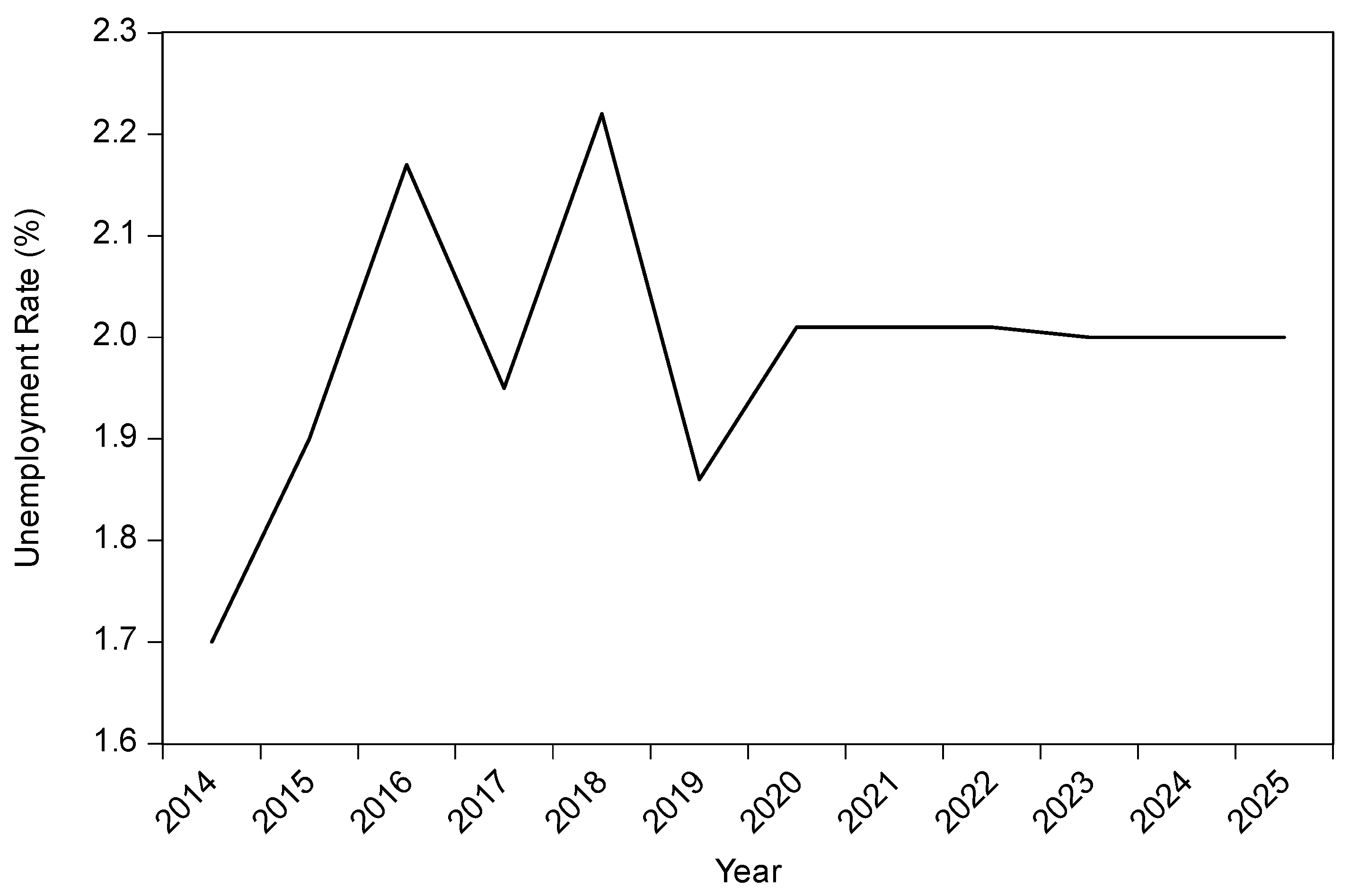
Figure 9 shows the unemployment rate for the rural area of the Highlands. Starting at 0.93% in 2014, the unemployment rate in the rural area of the Highlands region decreased to 0.76% in 2015. The year 2017 was quite similar to that of 2015 as the rate decreased to 0.69% from 0.88% in 2016. Finally, in 2019, there was a slight increase in the rate, from 0.88% to 0.94%. In the next six years, the trend is expected to increase to 1.18% in 2025.
According to
Figure 10, the average unemployment rate in the urban Southeast region during the period from 2014—2019 was about 2.88%, with the rate in 2015 being the highest, followed by the rates for the years 2014, 2018, 2019, 2017, and 2016. Then, in the following years, the unemployment rate for this region is expected to decline year after year to 2.79% in 2025.
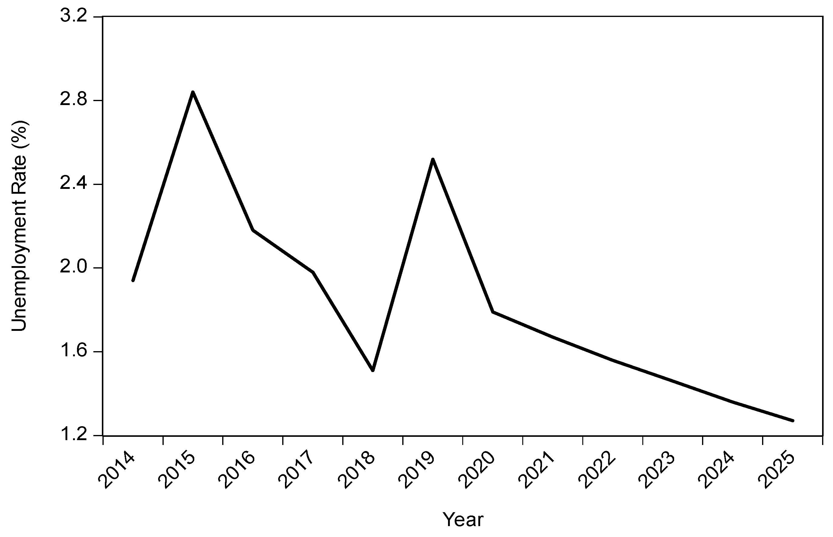
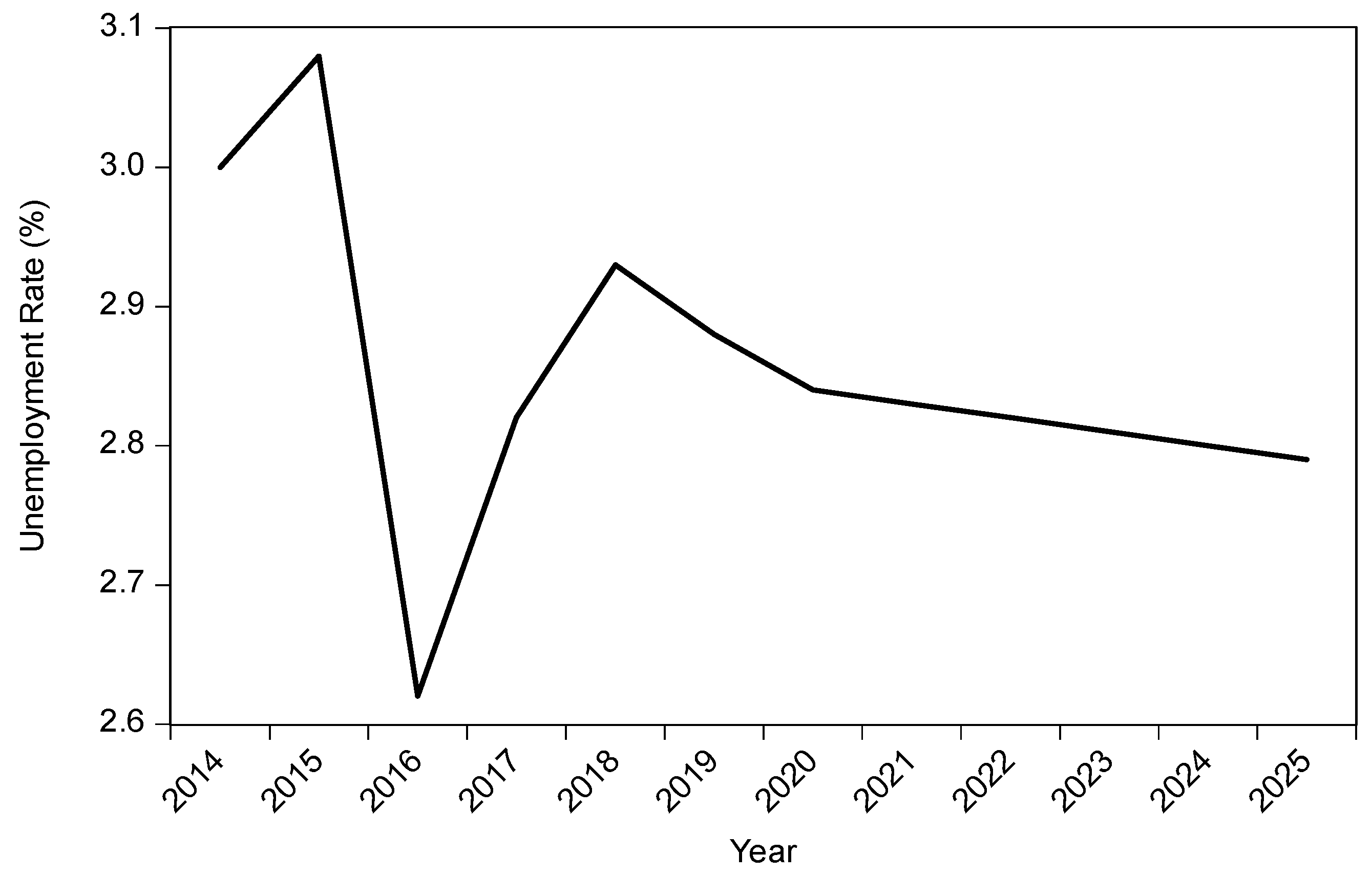
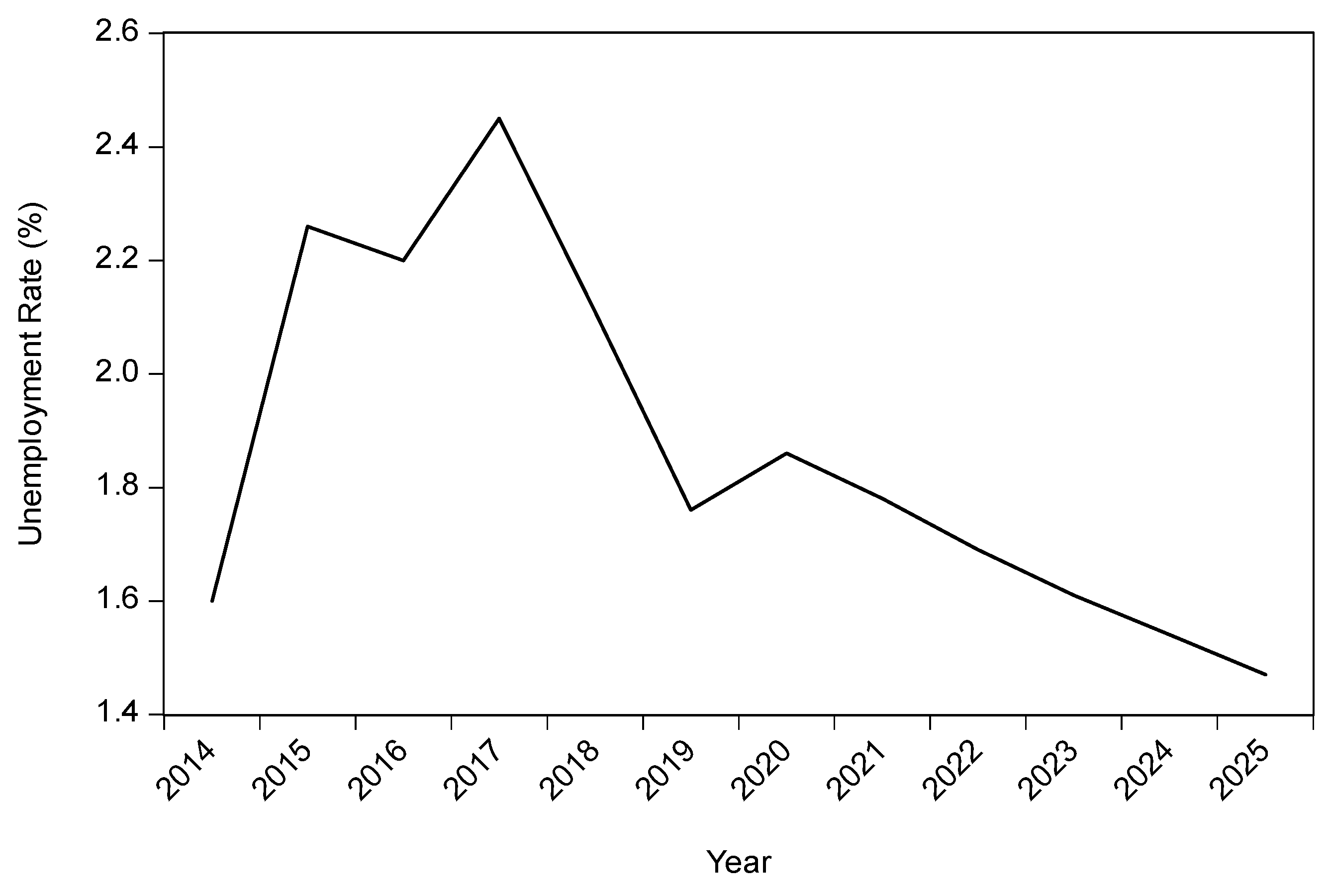
Figure 11 shows the unemployment rate for the rural area of the Southeast region. Between 2014 and 2019, the unemployment rate stood at 1.60% 2014. Then, there was a rise to 2.26% in 2015 before falling to 2.2% in the rural unemployment rate in the Southeast region in 2016. The rate then increased to 2.45% in 2017. From 2020 to 2025, the percentages for the unemployed in this region’s rural area are expected to decrease by 1.47%.
In
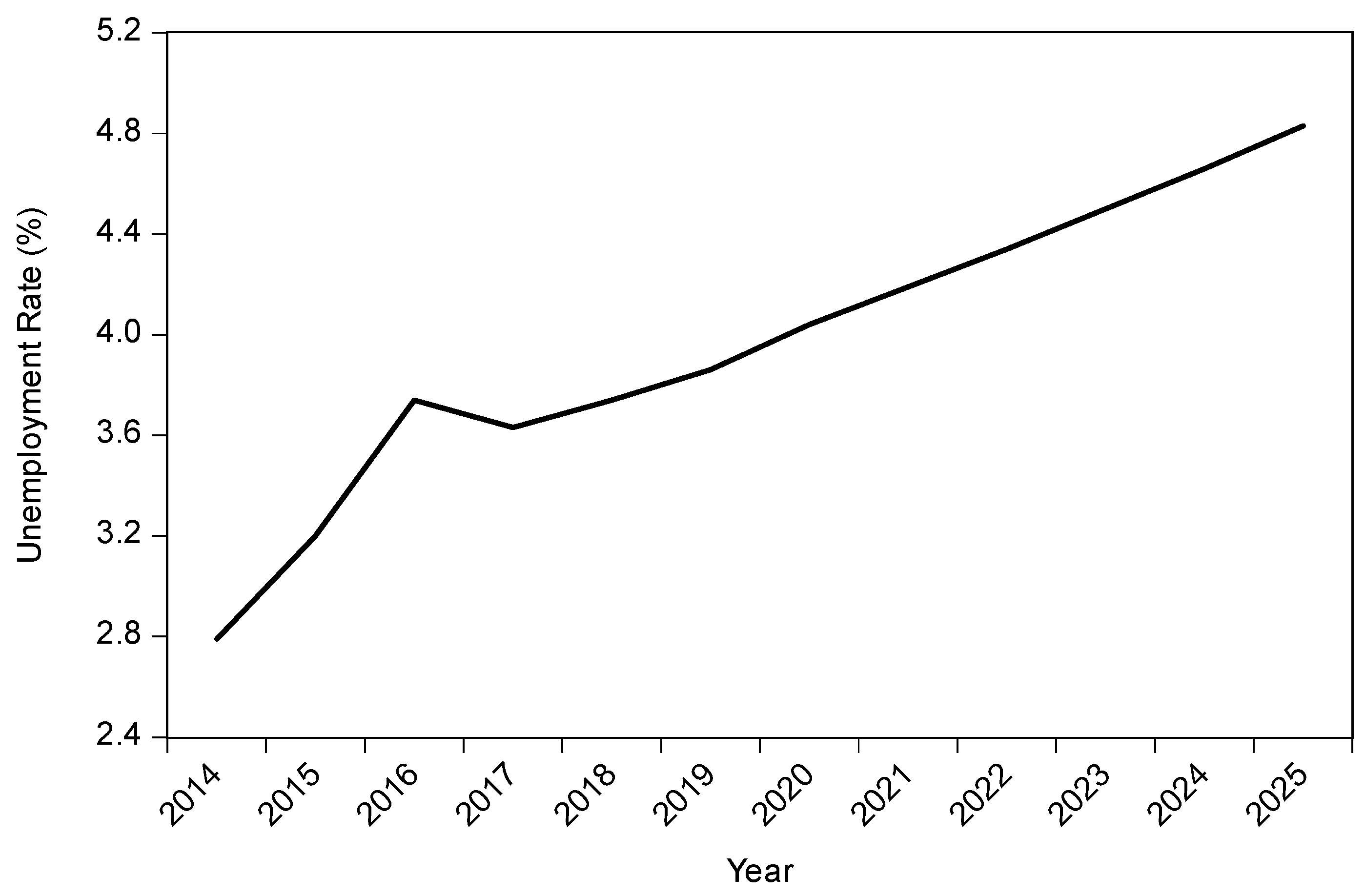
Figure 12, The Mekong River Delta’s urban unemployment rate, which increased from 2.79% to 3.74% in the first three years, decreased slightly to 3.63% in 2017. However, it continued its upward trend to 3.86% in 2019 and is expected to rise to 4.83% in 2025.
In the Mekong River Delta’s rural area, the unemployment rate was estimated at 1.83% in 2014. The unemployment rate maintained at around 2.6% during three years from 2015 to 2018, and then experienced a decline to 2.37% in 2018. Last but not least, the unemployment rate increased to 2.6%. Nevertheless, estimations indicate that the unemployment rate in the Mekong River’s rural area would continue to decrease until 2025, and by 2025 the rate could be around 2.31% in
Figure 13.
4.3. Comparative Analysis Results of the Proposed Models
The three models’ accuracies were tested through the MAPE. The performance of the proposed methods was investigated by comparing the initial values with and . Details about the calculations of can be explored in Equations (8), (17), and (21) for the GM (1,1), GVM, and ARIMA models, respectively.
According to
Table 4 for estimated data, it is clarified that the errors of GM (1,1) are more accurate in comparison to that of GVM and ARIMA models. The average MAPE values of 5.88% for urban areas and 5.16% for rural areas in
Table 4 are well fitted to the first level of the grade reference of the Grey prediction model, which is considered a highly accurate prediction. On the contrary, the MAPE values from the GVM and ARIMA models indicated significant errors (except HLR at the urban area in the ARIMA model) in the predictions for the future unemployment rate.
From
Table 4, it is apparent that the predicted values have the lowest mean percentage errors. For the North Central region, the lowest mean percentage error is roughly 1.76%, which means the forecast was completely accurate with an accuracy of 98.24%. Meanwhile, the Highlands region results had a mean percentage error of 14.73% from the ARIMA (1,0,1) model, indicating forecasted reliability of 85.27%. The remaining reliability test results for other regions revolve around 2.25% to nearly 9%, considered highly accurate forecasting for GM (1,1) model.
It is shown in
Table 4 that the mean percentage errors of the expected rural unemployment rate with GM (1,1) model in the North Central, Highlands, and Southeast Regions are relatively similar at 5.74%, 5.94%, and 5.57%, respectively. The Red River Delta’s figure is 4.53%, nearly twofold the number for the Mekong River Delta at 2.21%. However, the reliability test results of the estimated unemployment rates in the six regions are well fitted in the range of 1% to 10%.
Likewise, the MAPE results from the other administrative regions showed little-to-no errors in the GM (1,1) technique. This could be explained as, generally, the Traditional Grey Verhulst model could reflect the future unemployment rate; some defects in the model caused low predictions. This model indicated significant errors in the predictions for the future unemployment rate. However, the ARIMA model gave more successful forecastings than the Traditional Grey Verhulst model, except for RRD at the urban area and SER at the rural area.
As can be seen from the Appendices, the performance of the proposed methods was tested by comparing the initial values with
and
. Details about the calculations of
can be explored in Equations (8), (9), (16) and (17) for the GM and GVM models and in Equations (20) and (21) for the ARIMA model (
Appendix A,
Appendix B,
Appendix C,
Appendix D and
Appendix E).
Table 5 shows the unemployment rates for all regions’ urban and rural areas by using the GVM and ARIMA models. It is quite apparent that the unemployment rates for urban and rural areas would follow a downward trend until 2025 with the GVM model. On the contrary, the unemployment rates might steadily continue until 2025 with the ARIMA model.
Figure 14 shows the comparisons of the average forecasted unemployment rates in the urban and rural areas for the GM, GVM, and ARIMA models. According to the GVM model’s forecasting between 2020 and 2025, the average forecasted unemployment rates in the urban and rural regions will reach 0.79 and 0.42, respectively. However, the average forecasted unemployment rates with the ARIMA model in urban regions range from approximately 3.1%, whereas the figures for the rural areas are 1.62%. The diagrams between
Table A7 and
Table A12 show the unemployment rates in whole regions for six years from 2020 to 2025 using three forecasting methods, separately.


