
Development of an Urban Heat Mitigation Plan for the Greater Sacramento Valley, California, a Csa Koppen Climate Type

Altostratus Inc., Martinez, CA 94553, USA
Sustainability 2021, 13(17), 9709; https://0-doi-org.brum.beds.ac.uk/10.3390/su13179709
Submission received: 28 July 2021
/
Revised: 24 August 2021
/
Accepted: 26 August 2021
/
Published: 30 August 2021
(This article belongs to the Special Issue Urban Climate, Comfort and Building Energy Performance in the Mediterranean Climate)
Abstract
:An urban atmospheric modeling study was undertaken with the goal of informing the development of a heat-mitigation plan for the greater Sacramento Valley, California. Realistic levels of mitigation measures were characterized and ranked in terms of their effectiveness in producing urban cooling under current conditions and future climate and land use. An urban heat-island index was computed for current and future climates based on each location’s time-varying upwind temperature reference points and its hourly temperatures per coincident wind direction. For instance, the UHII for the period 16–31 July 2015, for all-hours averaged temperature equivalent (i.e., °C · h hr−1), ranged from 1.5 to 4.7 °C across the urban areas in the region. The changes in local microclimates corresponding to future conditions were then quantified by applying a modified high-resolution urban meteorology model in dynamically downscaling a climate model along with future urbanization and land use change projections for each area. It was found that the effects of urbanization were of the same magnitude as that of the local climate change. Considering the urban areas in the region and the selected emissions scenarios, the all-hours temperature equivalent of the UHII (°C · h hr−1) increased by between 0.24 and 0.80 °C, representing an increase of between 17% and 13% of their respective values in the current climate. Locally, instantaneous (e.g., hourly) temperatures could increase by up to ~3 °C because of climate effects and up to ~5 °C because of both climate and urbanization changes. The efficacies of urban heat mitigation measures were ranked both at the county level and at local project scales. It was found that urban cooling measures could help decrease or offset exceedances in the National Weather Service heat index (NWS HI) above several warning thresholds and reduce the number of heatwave or excessive heat event days. For example, measures that combine increased albedo and urban forests can reduce the exceedances above NWS HI Danger level by between 50% and 100% and the exceedances above Extreme Caution level by between 18% and 36%. UHII offsets from each mitigation measure were quantified for two situations: (1) a scenario where a community implements cooling measures and no other nearby communities take any action and (2) a scenario where both the community and its upwind neighbors implement cooling measures. In this second situation, the community benefits from cooler air transported from upwind areas in addition to the local cooling resulting from implementation of its own heat mitigation strategies. The modeling of future climates showed that except for a number of instances, the ranking of measures in each respective urban area remains unchanged into the future.
1. Introduction
Hot summer weather can cause a myriad of unwanted effects, including heat health impacts, increased cooling energy demand, higher emissions of air pollutants, and worsening air quality [1,2,3,4,5,6]. Thus, urban areas in the warmer parts of the world have implemented or have begun to implement various measures to combat heat. This study focused on the greater Sacramento Valley, California, and evaluated the potential benefits of urban cooling measures as a basis for developing a heat-mitigation plan by various organizations in the region. As this area is a Csa Koppen climate type, the focus of such plans is mainly on the summer season.
In this context, the goal of this and similar studies is to design and implement measures that reduce urban heat, not necessarily the urban heat island (UHI), per se. The UHI and UHI Index (UHII) are merely some quantitative yardsticks that indicate how much cooling can be reasonably expected at a given urban location. In other words, the UHI (or UHII) is simply an indicator as to how much cooling is needed to bring the temperature of an urban location down to that of a nearby non-urban area [7,8]. Of course, the actual cooling that is achievable at any given location could be smaller or larger than its assigned UHII [8]. In this article, a distinction is made between the UHI and UHII:
- UHI: Urban heat island is an instantaneous temperature difference between an urban location and a non-urban reference point (i.e., an instantaneous measurement). Thus, the units of UHI are °C.
- UHII: Urban heat island index is a cumulative temperature difference between an urban location and a non-urban reference point calculated over determined hours or time periods. The units of UHII are degree-hours per a certain time interval, e.g., degree-days or degree-hours. Thus, in this context, temperature is °C · h hr−1.
Of note, the urban heat indicators quantified in this study (including UHI and UHII) are air-temperature-based, not derived from skin-surface temperature, such as shown in many studies of “urban hot spots” that are satellite/thermal remote-sensing imageries, i.e., surface-temperature urban heat island. Hence, the spatial patterns of urban heat presented in this article differ from those seen in satellite imagery and can be counterintuitive in some cases.
Various cooling measures have been investigated in the past, e.g., Taha [1,9,10], Akbari et al. [11], Georgescu et al. [12], Gilbert et al. [13], and Levinson et al. [14], among many other U.S. and international studies, too numerous to list here. In this study, the following measures were evaluated and modeled:
- For area-wide urban cooling, that is, to achieve regional effects benefiting urban areas as a whole in the greater Sacramento Valley, the measures evaluated at the coarse (2-km) scale included the following: (1) cool roofs and cool pavements; (2) vegetation canopy cover; (3) combinations of measures; and (4) smart growth (for future climate), i.e., infill or greenfield developments.
- For localized effects at community scale, transportation corridors, roadway projects, and specific neighborhoods, i.e., to achieve localized benefits regardless of whether any actions were taken by other communities at the regional scale, the following measures were considered (these were modeled at a 500-m resolution): (1) cool roofs; (2) cool pavements; (3) vegetation canopy cover; (4) vehicle electrification; (5) solar PV; and (6) cool walls. In this article, a subset of these measures is discussed.
It is noted here that the urban-heat mitigation measures and mitigation levels proposed and modeled in this study are reasonable, i.e., they can already be found in the study region and are not hypothetical or extreme. In other words, one goal of this project is simply to encourage the wider use of materials and methods that already exist in the current market and in current construction and building practices in this area. Furthermore, keeping the modification levels reasonable also means minimizing potential negative effects on the atmosphere and urban environment, e.g., air quality impacts that could result from decreased mixing/venting, increased UV albedo, increased biogenic emissions, or concerns with the thermal/visual environments (Taha [9,15,16]).
Figure 1 provides a simplified introductory overview of the methodology and some of the overarching tasks.
2. Land Use and Land Cover Analysis
2.1. Study Region and Modeling Domains
The focus of this study is a region encompassing six counties in the greater Sacramento Valley, roughly covering an area of 32,000 km2, as shown in Figure 2. The modeling domain structure was configured based on nested grids of 54, 18, 6, 2, and 0.5 km in resolution. The 2-km grid was used to analyze the impacts of heat mitigation measures at the level of six counties. The 500-m grids, on the other hand, were used to evaluate the localized effects of mitigation measures at the project or community scales. These grids are as follows: D05: Yuba City/Marysville; D06: Woodland; D07: various areas in Sacramento; D08: Roseville and Granite Bay; D09: Folsom and El Dorado Hills; and D10: Placerville. The simulations were performed using the WRF modeling system with several components modified for high-resolution urban applications (discussed in Section 4).
2.2. Land Use/Land Cover (LULC), Urban Morphology, and Surface Properties Characterizations
To develop a detailed, bottom-up surface physical characterization input for the meteorological model, several data types were used. The datasets, ranging in resolution from 1 m to 30 m, included:
- National Land Cover Data for current LULC [17];
- USGS Anderson Level II and Level IV datasets [18];
- Google Earth Pro urban morphological and land cover data (google.com);
- Remote-sensed, area-specific building albedo characterizations [21];
- Earth Define/CAL FIRE urban tree canopy cover (www.earthdefine.com; accessed on 15 January 2020);
- Quick Bird UFORE urban tree canopy [24] *;
- NASA MODIS 7-band reflectivities (modis.gsfc.nasa.gov; accessed on 15 January 2020);
- Caltrans transportation datasets: www.dot.ca.gov/hq/tsip/gis/datalibrary *; accessed on 5 January 2020;
- SACOG regional land use (www.sacog.org/regional−gis−clearninghouse *; accessed on 15 November 2019);
- CalEnviroScreen environmental data: oehha.ca.gov/calenviroscreen [25]; accessed on 15 November 2019;
- Sacramento County general plan (www.per.saccounty.net; accessed on 20 November 2019 *;
- El Dorado County planning data: http://gem.edcgov.us/ugotnetextracts/ *; accessed on 5 January 2020, and
- Sacramento area building footprints: data−sacramentocounty.opendata.arcgis.com/ *; accessed on 2 November 2019.
- * Local data sources.
Based on these datasets, each model grid cell in D03 and finer was characterized bottom-up by calculating various parameters, including (1) vegetation attributes, e.g., cover, leaf-area index, height, geometrical properties, albedo, roughness length, and shade factor; (2) impervious cover, including roofs and ground-level paved surfaces and built-up fractions; (3) grid cell-level albedo from narrow-band reflectivities; (4) surface-specific albedo (roofs and pavements); (5) thermophysical parameters, including roughness length and soil moisture; (6) geometrical/morphological parameters including top-, plan-, and frontal-area densities, building heights, distribution of vegetation canopies, paved surfaces, sky-view factor, street widths and orientations; (7) heat emissions from buildings and industrial operations; and (8) vehicular traffic density and heat emissions [15].
3. Observational Weather Data
Observational meteorological data were used in (1) the initial characterization of the intra-urban microclimates in the study region, (2) the four-dimensional assimilation in the meteorological model, and (3) the statistical model performance evaluation. Several datasets were identified and used including: (1) NCEP-NOAA MADIS (Meteorological Assimilation Data Input System) with mesonet and urbanet; (2) National Weather Service/NOAA Cooperative Observer Program (COOP); (3) WeatherBug and Weather Underground CWOP; (4) NCAR dataset 472.0; (5) California Irrigation Management Information System (CIMIS); and (6) network-specific California datasets. The monitor locations (~400 stations) in the 6-counties area are shown in Figure 3. The data quality checks and uses are discussed elsewhere [15].
A detailed analysis of observed meteorology was carried out with some focus on the temperature field in the six-counties region, their localized tendencies, i.e., warming and cooling at each station, means, maxima, minima, ranges, and various indices, metrics, and derivatives [15]. To capture the area-wide characteristics, for example, Figure 4 shows the cumulative metrics for temperature, where YYYYMM denotes the year and month and DH day−1 (°C · h day−1) is the average for the given month (this is a non-threshold DH day−1 metric). In this figure, the progression of color codes from light to dark indicates lower to higher temperatures (the cooler zone in the northeast is the Lake Tahoe area). The observational analysis suggests significant background- and urban-generated heat in the region [15].
4. Urban Atmospheric Modeling
This work was carried out with the WRF modeling system [26] using Altostratus Inc.’s modified and updated urban canopy models, parameterizations, and data ingestion techniques (Altostratus AREAMOD and modUCM approaches) [8,15,27,28,29,30,31,32,33,34,35,36,37,38].
Very briefly, some of the Altostratus updates to the WRF model that were applied in this study include modifications to the urban canopy and land surface parametrizations, as well as to the single and multi-layer urban models so that they can be called simultaneously at any grid cell during model integration. The modifications also include adding the effects of vegetation and blue surfaces in the urban canopy model and the ability to specify hourly profiles and diurnal cycles of vegetation evapotranspiration or watering events that are location-specific. The WRF urban modules were also tested with a soil moisture model building upon earlier work with the urban MM5 [29,30]. Furthermore, trigger mechanisms call the urban parameterizations at specified locations (cells) based not on land use classes but on physical/geometrical properties of the built-up areas in each grid cell (see also Section 5.11.2). The flow-related parameters, e.g., roughness and length scales, are updated per wind direction and the corresponding frontal-area densities of building and green canopies, as well as the orientation of streets and canyons, where applicable. Altostratus also uses detailed, bottom-up, cell-specific characterizations of physical and geometrical properties including those of buildings, canopies, and other structures, as well as data preparation techniques that differ from those in the standard WRF pre-processing system. This results in more cell-specific characterizations of the surface. Various modules were updated to directly ingest these cell-specific parameters. The model options, physics, dynamics, and structure (vertical and horizontal) used in this study are discussed in Taha [15].
4.1. Base Modeling of the Six-Counties Domain (D04)
Figure 5 shows a random sample from the model field at 2 km, using the Altostratus modeling approach and depicting the higher temperatures in and around urban areas and the locations of mesonet stations and probing points relative to urban heat plumes. In this example, the field is for the all-hours average air temperature at 2 m above ground level for 15–30 June 2016. The range of average temperature (from light color to dark) is 13.6–28.6 °C, and each color level (step) is 0.5 °C.
Figure 6 is a random sample of results from a few hours in June 2013. It can be seen that the daytime urban heat plumes are pushed to the south and southeast by the northwesterly wind (Figure 6A) and to the east by westerly flow (Figure 6B). Figure 6C,D are sample snapshots from the model temperature field at 0700 PDT on two different days. Many areas are warmer than their surroundings, but for different reasons. The central parts of the domain are warmer because they are urban (the outlines of urban areas are clearly identifiable and the UHII effect is evident), whereas the eastern one-third of the domain is warmer because of the higher elevations (nighttime and early-morning inversions). This is also the reason why the Sutter hills (in the northwestern part of the domain) are warmer, as are the mountain ranges at the western boundary.
4.2. Model Performance Evaluation
At the 2-km level (see Figure 2), a model performance evaluation (MPE) was carried out for each year and interval at hourly time scales (each interval is 2 weeks long, after removing spin-up days). Variables that were evaluated at weather station locations (Figure 3) were (1) air temperature (°C), (2) specific humidity (g kg−1), (3) wind speed (m s−1), and (4) wind direction (°) [39]. Taha [8,15,27] discusses the benchmarks, metrics, and model performance for this region in California. Here, the mean absolute error (MAE) is presented briefly as example.
In this application, the air temperature’s MAE is 1.8 °C, which is within the recommended benchmark of ≤2.0 °C [39] and better than the 2–3 °C seen in a number of studies for California. In terms of specific humidity, the MAE is 1.2 g kg−1, also within the recommended value of ≤2 g kg−1. Wind speed statistics indicate an MAE of 2 m s−1, which is similar to the community-recommended benchmark of 2 m s−1. Finally, wind direction statistics show an MAE of 50° (within the recommended benchmark range of 30–60°). This is considered reasonable as it indicates a correct general flow direction. All of these indicators are satisfactory, especially considering the varied land cover and topography in the region and the wide range of atmospheric conditions in the study domain.
At the more local 500-m level (e.g., Section 5.11.3), MPE was carried out at those locations where urbanet or mesonet stations were sufficiently close to the project locations and for the selected time periods discussed in Section 5.11.1. The model performance with the modified urban parameterizations and special triggers approach used in this study (Section 5.11.2) further improved the model performance (MAE reduction) by 30–40% beyond the performance at the 2-km level listed above.
5. Effects of Mitigation Measures in Current Climate and Land Use
In this section, results are presented from (1) the modeling at 2-km resolution for the six-counties region to evaluate mitigation measures area-wide and (2) the modeling at 500-m scale to evaluate the potential benefits of localized measures at the community or neighborhood scales. Since this article focuses on urban heat, air temperature is the main subject of the analysis that follows. In Section 6, the effects of mitigation measures in future climates are discussed.
5.1. Characterization of the UHII in Current Climate
As introduced earlier, the greater Sacramento Valley is characterized by a Csa Koppen climate type and, as such, the focus of the mitigation measures is largely on urban heat during the summer. Thus, for this purpose, the months from May to September (MJJAS) of the years 2013–2016 were modeled and analyzed. Based on wind climatology, the six-counties region was divided into six “tiles” or sub-domains (Figure 7), each of which was assigned its own set of non-urban, upwind temperature reference points. The reason for assigning different and separate reference points for each sub-domain was to (1) cancel out the large-scale, regional climate signal, i.e., the changes in the background temperature across the region, and (2) to more accurately select non-urban reference points since the flow varies in direction among those tiles. For example, areas to the north of Sacramento (such as Yuba City/Marysville) are generally warmer than those southwest of Sacramento because the latter is influenced by the sea breeze from the San Francisco Bay Area, and this regional heat pattern is unrelated to urban effects (Figure 4, Figure 5 and Figure 6). Thus, using separate non-urban reference points for different tiles can compensate for these regional climate differences.
The UHII at any location (i.e., at each grid cell) within each of the six tiles was computed relative to a time-varying, wind-direction-dependent upwind reference point. The reference points for each tile were selected to be outside of the urban heat plumes per wind direction. This was determined from a model ensemble that characterized the plumes and their variations. This also took into account the temperature-change length scales discussed below in Section 5.5. Thus, at each hourly or sub-hourly interval of the simulations, the wind approach direction at each grid cell in the tiles was diagnosed, and the UHII was computed per upwind reference points for each tile independently of the others. This approach, while more accurate than the standard methodologies of using static reference points, can sometimes produce counter-intuitive spatial patterns of the UHI and UHII [8,15]. An example for all-hours UHII is shown in Figure 7 for the period 16–31 July 2015. The all-hours averaged temperature equivalent (i.e., DH hr−1) is as follows (for selected disadvantaged communities): A: 3.3 °C; B: 3.6 °C; C: 2.1 °C; D: 3.9 °C; E: 2.1 °C; G: 1.5 °C; and H: 2.7 °C. Other UHII temperature equivalents shown in this figure are Davis: 2.1 °C; Woodland: 1.5 °C; Yuba City: 2.2 °C; Placerville: 1.8 °C; Auburn: 4.5 °C; and Roseville-Lincoln: 4.7 °C. Recall, again, that each tile is independent of the others, even though they are plotted together on the same map shown in Figure 7.
In areas such as Auburn, Rocklin, and Lincoln, for example, the UHII can be elevated because of day/night variations in the temperature of the natural surroundings, higher elevations (Auburn), or heat transport from upwind urban areas (Lincoln and Rocklin). The latter effect can be explained with Equation (1) in that the change in air temperature (T) at any location (e.g., a point in an urban area) is the sum of (1) temperature change resulting from local heat generation or physical processes and (2) change resulting from transport of heat, e.g., from upwind urban areas, by the wind vector (u). The local heat generation could stem from anthropogenic origins such as motor vehicles emissions, building operations, and industrial activities, or result from heat fluxes exacerbated by surface physical properties of roofs, pavements, roadways, and so on.
Thus, if local heat generation were invariant at a given time interval, the change in temperature becomes proportional to heat transported to the location which, in turn, is proportional to the time and distance an air mass travels over an upstream urban area (for example) during that interval before arriving at the location of interest. Figure 8 shows an example of back trajectories arriving at three locations in the greater Sacramento region at 1400 PDT in the period 16–31 July 2015 (trajectories were computed with RIP4; www2.mmm.ucar.edu/wrf/users/docs/ripug.htm (accessed on 15 November 2019) and then plotted with GIS). While the wind direction varies from day to day and hour to hour, in this example, a significant percentage of the approach directions is from the southwest, i.e., from the San Francisco Bay Area.
Air masses travel over mostly natural and agricultural lands (Figure 8) before arriving at community C, but other masses travel slightly longer over urban areas before arriving at communities A and B. However, air masses arriving at Rocklin, for example, travel almost 4 h over urban areas before arriving there. Per Equation (1), this partly explains why the UHII is larger in communities A and B than in community C and also why it is significantly larger in Rocklin than in communities A and B. As will be discussed later, this is a reason why the reverse effect (cooling) also occurs, i.e., reductions in the UHII with mitigation measures, assuming region-wide deployment, are also larger in this direction.
UHII information, such as the data displayed in Figure 7, can then be processed further to generate derivatives for, say, planning or implementation purposes. As an example, one could characterize a temperature-weighted UHII that could be used in conjunction with other datasets such as CES 3.0 [25] to help prioritize geographical areas for the deployment of cooling measures. Thus, some qualitative scoring of areas can be developed based on both UHII and absolute air temperature, that is, areas with both a large UHII and high absolute temperatures receive a higher score than areas with a small UHII and lower temperatures. To develop a weighted UHII score, wuSCORE (here, for all hours and all intervals), a tier can be assigned to each of the UHII and absolute temperature ranges as follows:
- 1.0 ≤ UHII < 2.0, UHIItier = 1 25.0 ≤ Tair < 26.0, Tairtier = 1
- 2.0 ≤ UHII < 3.0, UHIItier = 2 26.0 ≤ Tair < 27.0, Tairtier = 2
- 3.0 ≤ UHII < 4.0, UHIItier = 3 27.0 ≤ Tair < 28.0, Tairtier = 3
- 4.0 ≤ UHII < 5.0, UHIItier = 4 28.0 ≤ Tair < 29.0, Tairtier = 4
- 5.0 ≤ UHII < 6.0, UHIItier = 5 29.0 ≤ Tair < 30.0, Tairtier = 5
where, the units of Tair are °C and the units for UHII are °C·h hr−1 (these ranges are specific to this region and the summer conditions during the studied periods). Then, the weighted UHII score (wuSCORE) for a given grid cell could be just their product, as follows:
wuSCORE = LOG (UHIItier × Tairtier)
The use of LOG in Equation (2) is simply to compress the range of wuSCORE for plotting and scaling purposes. The wuSCORE is dimensionless and has no physical meaning. Figure 9 is an example of wuSCORE computed based on both the all-hour UHII and all-hour absolute temperature averages for all years and intervals modeled in this study. Compare Figure 9 with Figure 7. Of course, this is a simple example that could be made more quantitative, or, instead of Tair, one could use virtual or apparent temperatures, solar radiation, the NWS heat index, or others.
5.2. Definition of Heat Mitigation Measures at the Regional Scale in Current Conditions
At the 2-km level, the mitigation scenarios were defined as follows:
- Case 10: A modest increase of 0.15 on average in albedo on impervious surfaces. Difference between this and the base case is labeled “del10”. †
- Case 20: Larger increase in albedo of 0.25 on average on impervious surfaces. Difference between this and the base case is labeled “del20”. †
† Note that the above increases in albedo are specified at the surface, e.g., roof or pavement. When averaged over urban grid cells in each area, the increases become small—between 0.01 and 0.03. Both case 10 and case 20 are realistic and reasonable, translating into the surface-specific caps (limits) on increases summarized in Table 1.
- Case 01: A first-level increase in canopy cover, about 2.5–3 million trees throughout the entire 6-counties region, which is about a 12% increase in cover, e.g., an additional 12% of a cell’s area on average. Previous studies [24,41,42] estimated that the established urban forest canopy in the Sacramento region is ~15% and that many urban areas have canopy cover that needs to be brought up from 2–5% to 15%, hence the 12% increase. The difference between this case and the base case is labeled “del01”.
- Case 02: An extreme level of increase in canopy cover (~20%–25% cover increase or adding 5–6 million trees throughout the entire 6−counties region). This is not a realistic scenario, nor is it considered feasible at this time, and thus, it is not used in the combined scenario (case31, below) and is excluded from some analysis later in this article. This scenario is included as a test for potential upper-bound effects per suggestions from local tree organizations that are targeting such increases in canopy cover, at least locally. Still, compared to findings from other studies, this increase is smaller than what is typically proposed (canopy increase of 35%–40%) to exert a significant impact on air temperature. The difference between this case and the base case is labeled “del02”. Taha [15] also models several intermediate levels of canopy cover to evaluate the incremental effects of growth (or additional canopy) on air temperature and water usage. These are identified here as 01A, 01B, 02A, and 02B.
- Case 31: This is a combination of realistic high albedo and canopy-cover increases. The increase in albedo is slightly larger than in case20, and the increase in canopy cover corresponds to that of case01. The difference between this case and the base case is labeled “del31”.
In this modeling framework, the effects of tree canopies (i.e., cases 01, 02, and 31 above and case B in Section 5.11.1) were parameterized via specifying and computing frontal area density, height, roughness length, albedo, evapotranspiration, soil moisture, shade factor, vertical profiles of foliage density (leaf-area index), and the properties of the surfaces underlying the canopy [10,15,24,29,41]. At the finer scales, where the urban parameterizations are triggered (discussed in Section 5.11 below), the canopy effects were additionally quantified using an urbanized sub-mesoscale soil model [43,44] building on previous work with the urban MM5 model [29,30,31,32,45]. As the focus of this study was on the urban climate and outdoor environment, as well as on the transportation system, these parameterizations of vegetation effects on the urban canopy, ground surfaces, and roadways were deemed appropriate. Had building energy use or indoor conditions been the top priority, other and more recent urban vegetation models [46,47] would have been considered as well. On the other hand, this also suggests that there were additional benefits from tree canopies, e.g., shading buildings and energy savings, that were not accounted for in this study.
At the 2-km scale, the canopies were implemented per technical potential indiscriminately as to where within each model grid cell they should be placed. At the 500-m scale, the trees were positioned per guidance from the local communities. At some locations, this was explicitly specified per local projects, such as in a transportation corridor, a bridge, a specific downtown area, etc. In other areas, the canopies were assumed to be distributed along roadways, over parking lots, in parks/open spaces, and residential/commercial lots. The distribution was determined per land use/land cover makeup and the urban morphology of each target model grid cell.
5.3. Minimizing Inadvertent Impacts on Biogenic Emissions, UV Albedo, Mixing, and Thermal/Visual Environment
As with many environmental control measures, the selection and implementation of urban cooling strategies can in some cases result in unintended consequences, that is, produce both positive and negative effects [7,10]. The opposing impacts can be seen in meteorology (e.g., cooling and warming), emissions (decrease and increase), and in air quality (e.g., decrease and increase in formation, transport, or mixing/concentrations of ozone or particulate matter) [15]. Here, some pointers to suggested considerations are listed:
- Impose constraints on albedo increase to prevent issues with glare and possible pedestrian visual/thermal discomfort at street level. Limit the maximum final albedo on roadways and pavements to 0.35 and on roofs to 0.50.
In this study, the competing positive and negative effects of mitigation measures were accounted for, and thus, the final results embody the various possible outcomes and compensating factors.
5.4. Impacts of Mitigation Measures on Wintertime Outdoor Air Temperature
Prior to proceeding with the quantification of summertime impacts from heat-mitigation measures, which is the main objective in this study, the potential wintertime effects of these measures (at the proposed levels of implementation) were also evaluated to ensure that no significant negative effects are imparted. Of concern are the potential penalties in terms of heating needs during the winter season, although this is not a major issue in the Csa Koppen climate type. For indoor air temperature, these effects would have to be evaluated on a building-by-building basis, but the impacts have been shown to be small in a climate such as that of the greater Sacramento Valley [53].
In this study, the effects of mitigation measures on wintertime outdoor urban air temperature were examined. The modeling and analysis show small or non-existent cooling effects in winter (a result of smaller solar altitude angle and larger cloud cover). The analysis suggests that the reasonable albedo-increase levels proposed in this study would result in no significant negative impacts during the winter [15] both in terms of the area affected by the temperature changes and the magnitude and duration of such changes. Higher levels of albedo increase (hypothetical and not modeled in this study) might result in more noticeable negative wintertime effects. As such it is important to constrain the albedo increases to reasonable levels—as defined earlier in Section 5.2 and Section 5.3. In terms of urban greening strategies, the same conclusion applies as over 70% of the trees in the Sacramento region shed their leaves in winter [15,54], thus reducing ambient cooling from shading and evapotranspiration. For evergreen trees, the lower incoming solar radiation (increased cloudiness and larger solar air mass) and lower air temperatures also reduce the trees’ cooling effects [15].
5.5. Estimation of a Length Scale for Cooling
In Section 5.12 and Section 6.7, the efficacies of urban cooling measures are evaluated under two scenarios: (1) when implemented in a community whose neighbors do not apply any heat mitigation strategies and (2) when implemented in a community whose neighbors also deploy urban cooling measures. Thus, some estimates of a length scale for cooling are developed in order to define the extent of upwind urban areas affecting a certain location or neighborhood as discussed in Taha [8,15]. Such length scales are also of relevance in the selection of UHI/UHII reference points and locating them outside of urban heat plumes as was introduced earlier in Section 5.1.
As expected, the length scale depends on the level of surface modification, weather conditions, wind speed and direction, the upstream distance over which an air parcel travels over hot or cooled surfaces (i.e., the size of the urban area), and the desired downwind temperature threshold, i.e., how large the temperature reduction is relative to an original upwind reduction value, ∆o, by the time it reaches the downwind point of interest. Several indicators could be used, for example, e-folding (1/e ∆o), half-life (½ ∆o), or some other measure. In this discussion, a temperature−reduction half-life (½ ∆o) is presented as an example, meaning the distance downwind where temperature reduction reaches half of the original temperature depression (∆o) at the edge of the cooled urban area [15].
Figure 10 is an example from this analysis (in this case using temperature difference corresponding to perturbations from case 10) at random time intervals with different flow patterns and wind directions. The cool-air plumes correspond to the coincident wind directions (depicted in the upper-left part of each figure). The small circles are grid cells where albedo was increased (the darker the circle, the larger the albedo increase, per legend on each figure). The shades of blue are the changes in air temperature—the darker blue means larger cooling. As can be seen, there are areas that have become cooler even though no local changes in albedo were applied. These are areas affected by the transport of cooler air from the modified grid cells upstream.
From the analysis over a range of wind speeds (per each direction), temperature reductions, sizes of urban areas in this region, and levels of mitigation, the half-life for temperature reduction (½ ∆o) was found at 2 to 4 km downwind (where ∆o is taken at the end of an airmass trajectory before exiting the urban land use). In other words, for the region’s current-climate summer conditions studied in this effort (MJJAS 2013–2016), an air mass cooled by flowing over an urban area where mitigation measures have been implemented can retain half of its cooling by the time it reaches 2 to 4 km downwind from the edge of the urban area (where temperature depression = ∆o). The lower bound is associated with the smaller urban areas and lower levels of mitigation, whereas the upper bound is associated with the larger urban areas and the higher levels of mitigation.
5.6. Effects of Mitigation Measures in Current Climate and Land Use: Example Instantaneous Temperature Differences
To begin the presentation of effects from various mitigation measures, a brief snapshot from the temperature-difference field is provided as an introduction. In Figure 11, the instantaneous temperature impacts of five mitigation measures are presented for the scenarios defined earlier in Section 5.2 and for a random hour at 1300 PDT, 28 July 2015.
The instantaneous temperature reductions reach up to 0.7, 1.4, 1.5, 2.4, and 3.9 °C for cases 01, 02, 10, 20, and 31, respectively. The spatial pattern of these reductions follows the urban boundaries as well as the downwind transport of cool air, as discussed in Section 5.5. The magnitude of cooling is also proportional to the built-up density and the size of the urban area being modified. Of note, the mitigation measures can also cause some warming, generally downwind of the modified urban areas. However, the warming is small compared to the cooling effect both in magnitude and the size of the areas affected by it. In this example, the warming can be seen mostly in the northeastern part of the domain (small areas shown in green), reaching up to a maximum of 0.3 °C on average.
5.7. Impacts of Mitigation Measures and Their Ranking at the Regional Scale
In addition to the instantaneous impacts discussed for example in Section 5.6, the effects of mitigation measures were also evaluated at other hours, periods, and ranges [15]. Here, two examples are presented, namely, for hours 1400–2000 PDT and the all-hours interval.
5.7.1. Impacts on the Temperature Field during Hours 1400–2000 PDT
This block of hours, especially in summer, is of interest to local utilities in peak electric load planning. In this interval, the effects of albedo measures are generally larger than those of canopy cover, excluding case 02. The magnitudes of reductions in temperature and the intrameasure differences within each area differ by location (Figure 12). There are also instances where the measures are tied in terms of cooling potentials (e.g., case 02 and case 20 in Woodland). This indicates that the effects of albedo are very significant during this range of hours and can even be equivalent to the effects of extreme canopy cover increases. The most effective measure overall in this interval is case 31.
5.7.2. Impacts on the All-Hours Temperature Field
Figure 13 shows the all-hours average temperature reductions, i.e., averaged over all hours in each period and also averaged over urban grid cells in the specified sub-domains. The ranking of measures is influenced by nighttime effects of vegetation cover and thus may not be a good indicator for use in daytime urban heat reduction. The areas of Davis, Sacramento, Woodland, and Yuba City see the larger cooling effects. The most effective scenario is case 02—if this scenario is excluded as an extreme, then the next most effective one is the combination measure (case 31).
5.8. Rankings in Current Climate
To provide an “at a glance” comparison among various scenarios, Figure 14 summarizes the rankings of the five measures in various areas and for different hours or times of day in current climate and land-use conditions. Cases that are tied are indicated by a repeated number and color code. The rankings are based on temperature changes averaged over 2 km. These rankings can differ at the finer scales (500 m) and the magnitudes of the temperature reductions also become larger when averaged at finer resolutions. In Figure 14, the various time blocks or bands may be relevant to different applications. For example, the 0600 PDT and allHRS bands could be of interest from a heatwave perspective, the 1400–2000 PDT band may be of interest to local electric utilities, the 1500−PDT band could be used in relation to peak cooling demand analysis, and the band at 1300 PDT is of relevance to assessments of measures that are most effective around solar noon. Figure 15 shows the temperature changes corresponding to Figure 14.
Modeling future climates (e.g., year 2050 RCP 4.5 and RCP 8.5, discussed later) shows that, except for a number of instances, the ranking (order) of measures in terms of their cooling effectiveness in current climates and LULC remains relatively unchanged in the future. However, while the order can be relatively similar in current and future years, the magnitudes of the cooling effects differ. It can be concluded from the analysis that albedo scenarios (e.g., cool roofs and cool pavements) are the top choice for reducing daytime urban air temperature. Because the vegetation canopy cover can cool the air both during the day and at night (albeit less so at night than during the day [35,36,37,38]), its impacts are dominant in the 24-h average metrics and the early-morning averages.
5.9. Impacts of Cooling Measures on the UHII in Current Climate
An overview is presented here for the regional scale (2 km)—a similar assessment at the fine scale (500 m) follows. The examples shown here are for cases 01, 02, 10, 20, and 31 for the all-hour average UHII. It is reiterated that the maps shown in this discussion are composites of six different tiles, each with its own upwind reference points. It is also noted that the changes discussed here are changes in the UHII (which, itself, is a temperature difference) not in absolute temperature.
Figure 16 depicts the potential offsets of the UHII as an all-hour average for a sample period 16–31 July 2015. It shows the spatial characteristics of the offsets which, again, are skewed relatively more towards the effects of canopy cover (since they include nighttime effects). One can see that (1) the spatial pattern of UHII mitigation is in general such that the greater offsets are generally in locations of larger UHII (which is desirable) and (2) that case 31 (as well as case 02) can offset most if not all of the all-hours UHII.
The most effective measures (excluding case 02) are the combination scenario and the vegetation-cover case 01. The albedo-only measures are still effective and significant, but because this metric includes nighttime effects, vegetation canopy has a more dominant effect. Figure 17 summarizes the reductions in the UHII (DH exceedances) relative to 35 °C, which is a threshold commonly used by the electric utilities in calculating summertime cooling loads. Excluding the extreme case 02 and related scenarios (02A,02B), the most effective measure is again case 31 followed by albedo (case 20) and vegetation-canopy cover (case 01).
5.10. Reductions in National Weather Service Heat Warnings in Current Climate
One of many beneficial aspects of urban cooling measures, at least in theory, is their potential to improve public heat health in summer. To characterize these benefits, the reductions in exposure above various warning levels of the National Weather Service heat index (NWS HI), were quantified. The NWS HI is computed based on both temperature and humidity and is reported as an effective temperature (in °F) [1]. Several metrics are discussed below that provide an assessment of these potential effects—they were calculated at a number of probing locations identified in Figure 18. As discussed below and shown in Table 2 and Table 3, the mitigation measures can also reduce the number of heatwave days and the exposure to heatwave conditions.
The NWS HI “Danger” level is defined above 106 °F (41.1 °C) and “Extreme Caution” above 91 °F (32.8 °C). The “Caution” level is set at 80 °F (26.7 °C), as shown in Figure 19. A heat wave is defined when the NWS HI is within or exceeds 105–110 °F for at least 2 consecutive days. Per this definition, and as seen in the figure (for 1700 PDT), the model correctly captures heat events/heatwaves in the region during the intervals of (1) 30 June–4 July 2013 (day counter 30–34 in Figure 19), (2) 30 June–1 July 2016 (day counter 345–346), and (3) 28–29 July 2016 (day counter 373–374).
The cooling measure (case 31) can shift down the index from one warning level to a lower one. Some such instances are seen at the locations of the green arrows (pointing up or down) where the NWS HI goes from the “Extreme Caution” level (blue series) to the “Caution” level (red series). Table 2 provides additional information for the hours at 1700 PDT in terms of exceedances and potentials for reduction by the mitigation measures (in this example, case 31). For each sample probing point (P0001 through P0028), the first three rows provide the percentages of DH above the given thresholds and the following three rows give the reduction (%) in DH above those thresholds, respectively. The analysis indicates that the mitigation measure has a significant impact—it can reduce exceedances above 106 °F (Danger) by between 50% and 100% (except for one location) and exceedances above 91 °F (Extreme caution) by between 18% and 36% [15].
In terms of locally offsetting the effects of excessive heat events or heat waves (per above definitions), Table 3 provides a summary of the mitigation potential for case 31. It shows (1) the number of days with NWS HI of 105–110 °F at each selected probing location for the three heatwave events identified above and (2) reduction in the number of heatwave days at each location as a result of implementing case 31. The heatwave effects are locally offset everywhere, except for one period in the Yuba City/Marysville area.
Figure 20 provides information for additional hours from 1400 to 2000 PDT. It summarizes the average reductions (percentage-wise) in DH exceedances above the 3 warning levels of the NWS HI for case 31 at 13 selected probing points (defined earlier) and for 7 individual hours (from 1400 to 2000 PDT), averaged over all such hours in the modeled periods (i.e., a total of 420 h for each computed average). If no data is shown for certain hours in the graphs, this means that there were no exceedances of the thresholds to begin with.
As seen in Figure 20, the mitigation measure can offset exceedances above the thresholds at all locations and hours, sometimes fully (100%) offsetting the exceedances over the “Danger” threshold. Furthermore, and except for the “Danger” level, the reductions in the other two levels exhibit a rough inverted “U” pattern, suggesting that the cooling measure reduces the heat index relatively more on both sides of the hour at 1700 PDT. That is, the NWS HI is reduced most (percentage-wise) at 1400 and 2000 PDT, followed by 1500 and 1900 PDT, then 1600 and 1800 PDT, and finally by 1700 PDT. Thus, in a way, the foregoing discussion of the hour at 1700 PDT might in fact have been a presentation of the more conservative beneficial effects of the cooling measure (i.e., the benefits can be larger at other hours, or it could be because the heat index was relatively smaller at those hours than at 1700 PDT).
5.11. Community-Level Impacts of Mitigation Measures
The goal of the fine-scale simulations at a 500-m resolution was to provide an assessment of the localized changes in microclimate resulting from project- or community-scale mitigation measures. In this section, a subset of the results is presented as example.
5.11.1. Definitions of Project- and Community-Level Mitigation Scenarios
- Case A: For Metro Transport Plan (MTP) projects, the roadway albedo was increased from an areawide mean of 0.12 (average of current roadway albedo) to 0.35 as a maximum per roadway. For the communities and urban areas identified by cities and project participants, roof albedo was increased from a current areawide mean of 0.17 to 0.5 as a maximum per roof and the roadway albedo to a maximum of 0.30 per roadway. The reason for imposing these upper limits was discussed earlier (Section 5.3).
- Case B: A vegetation canopy scenario that increases cover and evapotranspiration, but is different from canopy cover scenarios at the 2-km level (i.e., case 01 and case 02). Here, the increases in cover are applied to specific areas of interest defined by the counties and cities participating in the project. In this scenario, for example, some 325 large trees would be added to 0.25 km2 cells, which is roughly equivalent to an increase of 8% of a cell area. Thus, this is roughly equivalent to or smaller than case 01 in domain D04 (2 km grid), but the increase in cover is concentrated in a much smaller area.
- Case QF: In this vehicle-electrification scenario, heat flux from mobile sources was reduced by up to 25% in response to local studies that target an electric vehicle ownership level of 25% in the Sacramento region [40]. The base vehicular traffic hourly profile of anthropogenic heat emissions and its contribution to the total profile for the Sacramento area was computed per Sailor and Lu [55] and scaled in each affected model grid cell by roadways density. The maximum reduction of 25% in vehicular heat emissions’ contribution to the total emissions was further modulated and scaled down by (1) the distribution of roadways density in each grid cell and (2) the distance from charging stations [15]. The reductions in mobile-source heat emissions were evaluated along the major highways in the region.
For the community-scale modeling and analysis, the following periods are presented in this article:
- 1–15 July 2013: Example of hotter periods (daily max: 38–45 °C);
- 1–15 August 2016: Example of mid−range periods (daily max: 34–37 °C);
- 1–15 June 2015: Example of cooler periods (daily max: 27–35 °C).
5.11.2. Urban Parameterizations Triggers
As introduced in Section 4, Altostratus’s fine-scale modeling techniques include triggering various urban parameterizations based on surface physical properties and/or urban geometrical characteristics, not based on land use classification or “local climate zones” as is the standard approach in WRF. Of relevance to simulating the scenarios defined above, Altostratus also applies different urban parameterizations simultaneously in each grid cell, unlike the current practice in WRF where only one urban module is active during a model run. This can enhance quantifying the effects of various mitigation measures in different parts of each cell. Thus, for example, a 500-m grid cell might have an urban part that is a “canyon”, another urban portion that is not a canyon, a third part that is only slightly urbanized, and a fourth portion that is non-urban. In this case, three different urban parameterizations are triggered simultaneously in each cell along with the non-urban WRF. Thus, this is one way to represent further-resolved sub-grid-scale urban effects and capture finer-scale processes without the need to increase resolution beyond, say, 500 m (which is used in this study). The resulting fields and fluxes are then weighted by the respective built-up fractions, urban geometry, land cover/canopy physical characteristics, or flow properties [15,29,30,31]. Thus, the location- and site-specificity of the model results are enhanced.
Compared to a single active urban parameterization per model run (which is the standard approach in WRF), the multi-parameterization approach used in this study yields an improvement in location-specific model performance (especially for temperature) by up to 30–40% [15,27,30] at locations where observations from urbanet or mesonet are available (also see Section 4.2).
The determination of which parameterization to apply in different parts of a grid cell is done by thoroughly examining the makeup, surface properties, and urban geometry in each cell (which is part of the bottom-up approach to surface and morphometric characterizations) and via a tile approach evaluating whether an area in the cell lends itself to a high-rise configuration representation, a canyon geometry configuration, urban non-canyon, slightly urbanized, or simply paved/impervious with no buildings. These criteria are then used to trigger the different parameterizations during a model run. Furthermore, once urban parameterizations are triggered, cell-specific properties are then applied (from the bottom-up approach), unlike in the standard WRF where these properties are surrogated by land use type. These variables include the following (for each parametrization that is triggered): building heights, view factors, street widths, street orientations, impervious cover, building cover, frontal area densities, various vegetation cover attributes above and below the canopy, cell albedo, building and pavement albedo, and anthropogenic heat. These are then used internally by the model to calculate dynamics and physics variables.
5.11.3. Examples of Community-Scale Results
Two examples are presented here—domains D05 and D07. Other domains and results are discussed in Taha [15].
Domain D05 (Yuba City/Marysville)
Figure 21 depicts the MTP project locations and other areas of interest that were modeled to evaluate the local-scale impacts of mitigation measures in domain D05. The yellow line defines downtown Marysville, an area of interest per project participants, the orange lines are roadway and bridge projects identified by the city, and the red lines are MTP projects identified by local agencies. The major highways of interest for electrification scenarios are highlighted with bold black lines.
For case A (Figure 22, top left), both cool roofs and pavements are implemented in downtown Marysville, but in the MTP roadway project areas, only cool pavements are used. The urban canopy is cooled by up to a maximum of 4.5 °C at a few locations, as an average over all 1500−PDT hours in the period 1–15 August 2016 (in this example). The largest cooling is seen in the downtown Marysville area and in the MTP roadway projects in the southern part of the domain. For the roadway skin-temperature impacts of implementing cool pavements, the average maximum cooling (i.e., averaged over all 1500−PDT hours) in the period 1–15 August 2016 is 11.0 °C. For case B, the 24-h average cooling (in the sample interval 1–15 June 2015) reaches up to 1.8 °C in the north-central parts of downtown. For case QF, along the major highways in the area, namely, HWY 20, HWY 99, HWY 70, and HWY 65, the 1700 PDT (rush hour) average reduction reaches up to 1.8 °C during this sample interval. The largest cooling can be seen along highways 99 (N−S direction) and 20 (E−W direction) in Yuba City, as well as in downtown Marysville.
Table 4 is a summary of temperature changes for other hours or range of hours over the modeled periods identified earlier in Section 5.11.1. It is noted here (and in similar subsequent tables) that, unlike cool pavements and roofs, canopy cover affects air temperature above the canopy as well as both air temperature and surface temperature below the canopy. Similarly, for the electrification scenarios, the tail pipe exhaust occurs closer to the ground than to the upper parts of the urban canopy layer. Thus, for both canopy cover and electrification scenarios, it is more accurate to account for (e.g., average) both air and surface temperature changes, as will be shown later in the temperature summaries. However, for the purpose of Table 4 (and similar ones), the effects are reported separately. Of additional note, the largest cooling from vegetation during the daytime occurs earlier in the morning and later in the afternoon. Thus, the sample hours (1300 and 1500 PDT) in the table may not represent the largest effects from urban greening.
Domain D07 (Sacramento).
In Figure 23, the locations of interest in the Sacramento area are identified. The yellow zones are disadvantaged communities (AB617) [40]. The red lines are MTP projects and the major highways of interest in electrification scenarios are highlighted with bold black lines.
For case A, the urban canopy air temperature impacts are shown for a sample interval 1–15 August 2016 (Figure 24, top left). It is assumed that in the disadvantaged (AB617) communities (yellow areas in Figure 23), both cool roofs and cool pavements are implemented, whereas in the roadway project corridors (red lines), only cool pavements are applied. The average cooling in the urban canopy reaches up to a maximum of 5.2 °C at some locations as a result of implementing cool roofs and pavements (as an average over all 1500 PDT hours in this period). The largest cooling is seen in various parts of the communities as well as along the MTP roadway projects. Again, it should be re-emphasized that these cooling effects are significantly larger than those at the 2-km scale because they are very localized within the canopy layer and averaged over much smaller areas. The roadway temperature impact of implementing cool pavements averaged over all 1500 PDT hours in the period 1–15 August 2016 is 13.2 °C.
In case B, the increases in canopy cover were assumed to be implemented in communities A in the north and C in the south (Figure 24, bottom left). The 24-h average cooling (during the sample interval 1–15 June 2015) reaches up to 1.4 °C in community C and is larger than the cooling attained in community A. For case QF, in terms of the near-surface temperature effects from vehicle electrification, the model results along the major highways—I-80, HWY 50, I-5, and HWY 99—suggest a 1700 PDT (rush-hour) average reduction in temperature of up to 2.4 °C, during the sample interval 1–15 July 2013. The largest cooling occurs along HWY 50 and HWY 99, although all major highways do see significant cooling at different locations.
Table 5 provides a summary of temperature changes averaged (for different hours or range of hours) over the three sample periods identified in Section 5.11.1. The notes preceding Table 4 also apply here to Table 5.
5.12. Local Offsets of the UHII in Current Climate
Effects from deploying cooling measures at community scale (500 m) were compared to the corresponding local all-hours UHII in current climate. For this purpose, the local offset of the UHII via each mitigation measure was evaluated for two situations, as in Figure 25: (1) a scenario where only the community implements urban cooling measures (second to last column) and (2) a scenario where both the community and its neighbors implement cooling measures (last column). In this second situation, the community benefits from cooler air transported from upwind areas (that have implemented case 31, in this example) in addition to local cooling resulting from the implementation of its own heat mitigation measures (Equation 1). Length scales, or upwind distances of relevance to transport of cooler air, were estimated with an average half-life at 2–4 km (Section 5.5).
In Figure 25, the all-hours UHII and the all-hours offset of UHII at the 500-m resolution were averaged over the periods defined earlier in Section 5.11.1. It can be seen that (1) some measures, even in a standalone fashion, can completely offset the UHII, with or without the transport of cooler air from upwind urban areas, and (2) when neighboring communities also implement urban cooling measures (case 31, in this example), the local benefits increase significantly, sometimes more than doubling or tripling the effects.
It is to be re-emphasized that these are localized effects, i.e., temperature changes at or near the surface of the modified roadways or the effective air temperature within the urban canopy of the selected communities. Hence, the cooling effects of pavements alone (in some locations) can be larger than the effects of pavements and roof albedo modifications because the levels of increase in pavement albedo for the main highways and freeways are larger than those for the local roadways in the selected communities (for the reasons stated earlier). In addition, there is a shading effect in the urban canyons that reduces the efficacy of cool pavement measures [15,29,30,31,56].
6. Urban Heat and Mitigation in Future Climate and Land use
The changes in urban heat and its indicators (e.g., UHI, UHII, and other metrics) in response to changes in climate and urbanization levels were quantified. This was followed by an evaluation of the efficacies of heat mitigation measures under those future conditions. For this purpose, the year 2050 was selected per input from the regional air districts and local communities in the Sacramento Valley. Future local climate scenarios were generated via dynamical downscaling of the CMIP5/CCSM4 climate model [57] with Altostratus Inc.’s high-resolution customized urbanized WRF parameterizations discussed earlier, accounting for future urban surface physical properties and morphological projections, future changes in the transportation system, roadways, and infrastructure. Two representative concentrations pathways (RCP) for year 2050 were modeled: RCP 4.5 and RCP 8.5. These RCPs are defined in Clarke et al. [58] and Riahi et al. [59].
CCSM4 was used in this study, as it is one of ten climate models recommended by the California Energy Commission and the California Natural Resources Agency and is a “middle-of-the-road” model in terms of predictions. Furthermore, per Bruyere et al. [57], CCSM4 has been bias corrected using the NCEP/NCAR Reanalysis (NNRP [60]) as follows:
where CCSM4bc represents the bias-corrected climate model fields and Equations (3)–(5) are six-hourly. The average NNRP term in Equations (4) and (5) is taken over the period from ~1980 to 2005.
Analysis of the climate and meteorological models’ fields for 2050 (RCP 4.5 and 8.5) shows that it is generally significantly warmer than the current climate, as discussed in the following sections. It is also a middle of the road time frame.
6.1. Projections of Future Urbanization and Effects
In this study, the USGS LUCAS land use projection data [19,20] were vectorized and remapped to develop surface characterization input to the atmospheric model, including physical properties in areas that will be urbanized by 2050. Figure 26 depicts the projected urbanization in the greater Sacramento Valley by 2050 under the BAU scenario [15]. The green color-coded grid cells are the current urban land use [17] and the pink cells are the new urban areas by 2050. In this domain (D04), the urbanized area in 2050 is 68% larger than in 2015.
The next step was to develop physical characterizations for the new urban areas to update the corresponding input to the land surface and atmospheric models. Since it is unknown what the physical and geometrical characteristics of these new urban areas could be, this study simply assumed that they would be similar to the properties of existing nearby urban areas, i.e., near the outskirts of the current urban boundaries. Thus, an algorithm was designed to march through each new urban grid cell by 2050 and within a specified radius of influence, e.g., 6 km, search for current neighboring urban cells and average their physical properties. These properties were then projected onto the expanding, new urban areas (cells).
In Figure 27, a snapshot of the temperature change (i.e., temperature equivalent DH hr−1 of the UHII) in 2050 RCP 8.5 at a random single hour (1600 PDT) relative to the corresponding time and date in 2015 is presented. The range of change at that hour relative to current conditions (dark green to dark red, in the left figure) is +1 to +5 °C. In the new urban areas (outskirts seen in pink in Figure 26), the change is up to +5 °C, which can be attributed to effects of both climate change and urbanization, whereas the change in the existing (2015) urban areas is up to 3 °C, which is attributed to only the climate effects (since urbanization is assumed to not have changed noticeably in these areas). Thus, qualitatively at least, at this random hour, it can be said that the effects of climate are to warm the current urban areas by 3 °C, whereas the effects of urbanization (changes in land use only) are a warming of 2 °C. This implies that (1) changes in urbanization and LULC are critical to account for and consider when developing regional land use plans (since they have relatively similar local warming effects as the changes in climate) and (2) that urban cooling measures will be critical in the future as they can locally offset the effects of climate change.
An examination of all intervals, not just a single average hour as in the forgoing example, suggests that in the longer term, the local effects of changes in land use and in climate on air temperature are of similar magnitudes. For example, Figure 27 (right) shows the temperature equivalent (DH hr−1) of the UHII change for all hours during the period 16–31 July of 2050 versus the same interval in 2015. In this case, the climate effect is +1.36 °C and the land use effect is up to +1.41 °C (that is, 2.77 minus 1.36 °C), essentially of the same magnitude. Hence, the role of LULC change in warming and the role of heat mitigation measures in cooling (under current and future climates) should be fully acknowledged and explored in light of such similarities in magnitudes. Note, again, that Figure 27 (right) is a composite of six tiles that were defined earlier in Section 5.1.
6.2. Impacts of Climate and Land Use Changes on the UHII
The characteristics of the future UHII are dictated mainly by the effects discussed above, i.e., (1) local climate change and (2) urbanization. Table 6 is a summary of the average all-hours UHII (averaged over all JJAS intervals, not just the sample periods discussed above). It is noted from the table, and Figure 28, that the UHII is larger in 2050 RCP 4.5 than in current climate, and it is also larger in 2050 RCP 8.5 than it is in 2050 RCP 4.5, both of which are expected, except for domains D05 and D06. In these domains, the UHII in the RCP 8.5 scenario, while still larger than in the current climate, is slightly smaller than in RCP 4.5. The reason for this is that the non-urban areas surrounding Yuba City/Marysville (in D05) and Woodland (in D06) warm up faster in the long run than the urban areas as a result of lower vegetation cover in the non-urban surrounds (Taha [15]). Thus, by definition, the UHII becomes smaller, despite the absolute urban temperatures being higher in RCP 8.5 than in RCP 4.5. This phenomenon was also discussed in Taha [8] for various areas in California. Figure 28 summarizes the differences in future UHII relative to present.
6.3. Impacts and Ranking of Mitigation Measures in Future Climate and Land Use
Because the urban area will have expanded further by 2050, there is now increased technical potential, i.e., additional areas available for implementation of urban cooling measures. This translates into larger overall possible cooling and thus provides a counterbalance to the warming effects from both climate change and urbanization. In addition to the cases defined in Section 5.2, this study also evaluated a scenario of smart growth whereby 15% less urbanization occurs in the future (2050) relative to the BAU urbanization scenario discussed above. A range of metrics and hours were analyzed to quantify these effects [15]. Here, two examples are presented, namely, 1400–2000 PDT and the all-hours indicator.
6.3.1. Impacts of Mitigation Measures on Temperature during Hours 1400–2000 PDT
Figure 29 depicts the average temperature reductions, at sample locations, for the interval 1400–2000 PDT (i.e., temperature reductions averaged over all 1400 to 2000 PDT hours in each listed period) and also averaged over urban grid cells in each specified sub-domain. The figure also shows the ranking (i.e., the order of measures’ effectiveness) at this time interval labeled on the right side of each graph (which differs from that at other hours). During 1400–2000 PDT, the effects of albedo measures are larger than those of canopy cover, excluding case 02. The magnitudes of reductions in temperature and the intra-measure differences within each area also differ by location.
In this and similar figures, the sample intervals (int#) are as follows, int1: 1–15 June; int2: 16–30 June; int3: 1–15 July; int4: 16–31 July; int5: 1–15 August; int6: 16–31 August; and int7: 1–15 September.
The smart growth scenario was compared to the LUCAS BAU urbanization in the year 2050. These impacts are presented (in Figure 30) for those locations where urbanization was prevented [15]. The avoided warming (at these locations) ranges from an average of 0.6 °C in Davis to up to an average of 1.2 °C in Auburn. However, if averaged over each subdomain as a whole, the effects of smart growth become much smaller, namely, an avoided warming of between 0.05 and 0.15 °C region-wide.
6.3.2. Impacts of Mitigation Measures on All-Hours Average Temperatures
Figure 31 shows the all-hours average temperature reductions that are also averaged over urban grid cells in each specified sub-domain. The ranking of measures is uniform across most regions, but differs in Sacramento and Woodland. In the all-hours average, the effects of vegetation canopy are more dominant since they include nighttime hours.
The smart growth scenario was also evaluated for the all-hours average impacts and compared against those of the BAU growth in year 2050. Again, the impacts are presented here only for those grid cells where urbanization was avoided. Figure 32 shows that except for Auburn and El Dorado Hills, there is less variation across the regions and a relatively similar avoided warming of between 1.2 and 1.6 °C relative to if these areas became urbanized. When averaged over each sub-domain as a whole, the avoided warming becomes smaller, as discussed earlier.
6.3.3. Ranking of Measures in Future Climate and Land Use
Figure 33 summarizes the rankings of measures discussed above (excluding smart growth) for 2050 RCP 4.5 and RCP 8.5 and provides a comparison with their order under current climate and land use. The chart is color-coded so that black is most effective measure (largest cooling) and near-white is smallest cooling effect. Note that these are impacts on air temperature, not the UHII.
The following observations can be made regarding future rankings and how they compare to those in current climate:
- At 0600−PDT:
- ◦
- The rankings of mitigation measures (order) are similar and consistent across all regions;
- ◦
- Within each region, the rankings are similar across current and future climates;
- At 1300−PDT:
- ◦
- The rankings are different across the regions;
- ◦
- In Davis and Sacramento, the rankings also differ in future compared to current climate;
- At 1400–2000 PDT interval:
- ◦
- The rankings are different across the regions;
- ◦
- In Woodland, the rankings differ in future climate compared to current conditions;
- At 1500 PDT:
- ◦
- The rankings are different across the regions;
- ◦
- In Auburn, Davis, El Dorado Hills, and Yuba City, the rankings are different in future climate compared to current conditions;
- At all−hours interval:
- ◦
- The rankings are different across the regions;
- ◦
- Within each region, the rankings are similar across current and future climates.
The chart also shows that there are no differences in the order between RCP 4.5 and RCP 8.5 (but their rankings can differ from those under current climate). However, it is important to keep in mind that while the rankings may be similar in RCP 4.5 and RCP 8.5, the absolute changes in temperature and UHII are different.
6.4. Impacts of Mitigation Measures on the UHII in Future Climate
Two examples are presented for the effects on the UHII in future climate and land use.
6.4.1. Impacts of Mitigation Measures on the 1500 PDT UHII in Future Climate
Figure 34 summarizes the reductions (percentage-wise) in the 1500 PDT UHII averaged for all periods in 2050. The results show varying effects across scenarios and regions but also that, in general, the mitigation measures reduce the UHII in RCP 8.5 slightly more than in RCP 4.5. The ranking of measures at 1500 PDT (including the extreme case 02) is in the following order: 31, 02, 20, then 10 and 01 tied, in all sub-domains and is the same in both RCP 4.5 and RCP 8.5. This ranking (order) of measures is different from that at night or early morning—here, the albedo scenarios are more effective. As seen in the figure, there also is a single instance (anomaly) in Davis in RCP 4.5, where case 10 causes a very small (1%) increase in the 1500 PDT UHII and a case in RCP 8.5 in Woodland where case 01 has almost no effect on the UHII at this hour. This is also related to the long-term changes in non-urban temperatures in these regions, as discussed in Section 6.2.
6.4.2. Impacts of Mitigation Measures on the All-Hours UHII in Future Climate
In Figure 35, the reductions are shown for the all-hour UHII averaged for all periods in 2050. The results indicate that the reductions are almost identical in RCP 4.5 and 8.5 (for each respective region) but that minor differences occur and that the reductions in RCP 8.5, percentage-wise, can be slightly smaller than those in RCP 4.5. The ranking of measures for the reduction in all-hours UHII (including extreme case 02) is in the following order: 02, 31, 01, 20, and 10, in all sub-domains and in both RCP 4.5 and RCP 8.5. This order of measures is influenced by the effects of vegetation canopy cover, as this also includes nighttime effects.
6.5. Changes in the National Weather Service Heat Warnings in Future Climate
Changes in the NWS HI resulting from changes in climate and urbanization and the impacts of mitigation measures on the index were evaluated at the same probing locations defined earlier. In this section, examples are provided for changes at 1700 PDT, i.e., averaged over all 1700 PDT hours in the period JJAS of 2050 for RCP 4.5 and RCP 8.5 for case 00 and case 31 at location P0001 as an example for comparison with the first part of Section 5.10. The future-year NWS HI and its changes were compared to the corresponding values in the current climate (2013–2016), as seen in the sample Figure 36 and Table 7, where the percentages of reductions in exceedances are given relative to thresholds “Danger”, “Extreme caution”, and “Caution”. The mitigation measure can reduce exposure above the “Danger” level in both RCPs. It can also shift down exposure above “Extreme caution” to “Caution” as seen in the hours around counter 17, 53, 72 in RCP 4.5 and around counter 24, 67, 100, and 104 in RCP 8.5. Table 7 provides additional information for other sample locations.
6.6. Impacts of Mitigation Measures on Temperature Exeedances Relative to Threholds in Future Climate
The changes in temperature, e.g., cumulative DH, above certain thresholds in the future were evaluated along with the potential reductions resulting from cooling measures. In this section, a threshold of 35 °C is used as an example. Figure 37 depicts the percentage-wise reductions in degree-hour (°C·hr) exceedances above 35 °C in the sample subdomains, for all modeled time intervals (JJAS 2050), and for RCP 4.5 and RCP 8.5. For each time interval, the changes are presented for five scenarios. As before, the caveat related to case 02 (as an extreme measure) should be reiterated.
There is significant variation in the reduction of exceedances across different time intervals within each domain and variations from RCP 4.5 to RCP 8.5 within each region. There are also several cases (in different areas) where no exceedances occur above 35 °C in RCP 4.5, but significant exceedances are seen in RCP 8.5. As a result, the figures may be misleading in these cases suggesting larger reductions in RCP 8.5 when there are none in RCP 4.5 (because there are no exceedances in RCP 4.5 to begin with).
The ranking (order) of measures in terms of effectiveness is as follows (similar in both RCP 4.5 and 8.5): in Auburn: 31, 02, 20, 01, 10; in Davis: 31, 02, 20, and 01/10 tied; in El Dorado Hills: 31, 02, 20, 01, 10; in Placerville: 31, 02, 20/01 tied, and 10; in Sacramento: 31, 02, 20, 01/10 tied; in Woodland: 31, 02/20 tied, 01/10 tied; and in Yuba City: 31, 02, 20/01 tied, then 10.
6.7. Local Offsets of the UHII in Future Climates
The 500-m simulations were examined in the context of future climate (2050) with a goal of evaluating the effectiveness of localized measures in offsetting the future UHII. Figure 38 (for RCP 4.5) and Figure 39 (for RCP 8.5) are structured in a manner similar to Figure 25 (in Section 5.12), but for future climates and land use.
The model results indicate that the effectiveness of mitigation measures in 2050 is generally similar to their effectiveness in current climate. In other words, the UHII offsets (percentage-wise) for various measures are of the same magnitudes in 2050 (RCP 4.5 and RCP 8.5) as they are in current climate (compare with Figure 25). The reason for this, as explained earlier, is that increased urbanization, while contributing to significant additional local warming, also means an increase in technical potential, i.e., area available for the deployment of mitigation measures, thus keeping the overall UHII offset levels relatively similar to those in current climates or even slightly larger in some cases. Recall that these are localized impacts of mitigation relative to future UHII, not future absolute temperature.
7. Conclusion and Qualitative Takeaways
In conclusion, the following qualitative takeaways are provided, in no particular order:
- Significant urban heat exists in the greater Sacramento Valley. The UHI and the UHII are larger in urban areas that (1) are more densely built up, (2) cover a larger geographical area, (3) are located downwind of an urban zone, (4) are located at higher elevations, and (5) are surrounded by non-urban areas that cool down significantly faster at night.
- While temperature in the region generally increases from current climate to future (e.g., to 2050 RCP 4.5 and then to 2050 RCP 8.5), the corresponding UHII also increases in this direction, except for two urban areas where the UHII can be smaller in RCP 8.5 than in RCP 4.5 (although still larger than in the current climate). This is a result of faster long-term warming in the surrounding non-urban areas.
- It is highly feasible to mitigate the current and future UHI and offset the UHII (in some cases completely) using materials and practices that are reasonable and readily used throughout the region. The proposed urban cooling measures are reasonable—meaning they do not require extreme implementation levels, only what is already available and used in the current market and current construction and building practices in this area.
- Mitigation measures can offset the local UHII in standalone fashion, in some cases completely. Various combinations of measures can further offset the UHII, although the combined effects of measures are not linear and generally smaller than the sum of cooling effects from individual measures.
- The mitigation measures can have significant beneficial effects in terms of public heat health as indicated by their ability to lower exceedances above warning levels of the National Weather Service Heat Index. The cooling measures can also significantly reduce or completely erase the number of heatwave days during several excessive-heat events identified in the study.
- The mitigation measures are as effective under conditions of future climate and land use as they are under current conditions.
- Different mitigation measures affect urban heat and temperature differently during different times of the day. Hence it is possible to target certain time intervals, e.g., peaks, night, day, or all hours (per a community or city’s needs), if so desired, by choosing a specific mitigation measure or combinations of measures that are most effective during the desired time periods.
- If, in addition to a community’s own heat mitigation actions, neighboring communities also implement urban cooling measures, the local cooling effects could be significantly larger, sometimes by more than double or triple the amount (although there is a wide range of effects depending on location, time, and specific measures).
- Some measures that are not often associated with urban cooling (or urban heat island mitigation), such as vehicle electrification, solar PV installations, and smart urban growth, all appear to have significant beneficial urban cooling effects.
- The cooling effects are significant across a range of urban areas in the study region, including disadvantaged communities, which can help improve the thermal environment, reduce emissions of air pollutants, and improve air quality, especially in vulnerable areas.
A ranking of measures’ efficacies was done for each region, measure, and time interval (e.g., specific hours or a range of hours) for current and future climates and land use. Some areas or time intervals have a consistent ranking (order) of measures, others vary by location, and, yet, others vary in future climate relative to current conditions.
Funding
This article describes work that was performed with funding and support from the California Department of Transportation (Caltrans). The Sacramento Metropolitan Air Quality Management District (SMAQMD) is acknowledged for funding and managing this project. The local Government Commission (LGC) is acknowledged for directing the work. The findings and recommendations from this study do not necessarily represent the views of Caltrans, SMAQMD, LGC, or the State of California, nor do these agencies or the state assume any legal liability for the information generated in this work.
Institutional Review Board Statement
Not applicable.
Informed Consent Statement
Not applicable.
Data Availability Statement
Data locations were reported throughout the article.
Conflicts of Interest
The author declares no conflict of interest.
References
- Taha, H. Cool cities: Counteracting potential climate change and its health impacts. Curr. Clim. Chang. Rep. 2015, 1, 163–175. [Google Scholar] [CrossRef]
- Alfaro, E.; Gershunov, A.; Cayan, D.; Steinemann, A.; Pierce, D.; Barnett, T. A method for prediction of California summer air surface temperature. Eos Trans. AGU 2004, 85, 553–558. [Google Scholar] [CrossRef] [Green Version]
- Alfaro, E.; Gershunov, A.; Cayan, D. Prediction of summer maximum and minimum temperature over the central and western United States: The role of soil moisture and sea surface temperature. J. Clim. 2006, 19, 1407–1421. [Google Scholar] [CrossRef]
- Founda, D.; Santamouris, M. Synergies between urban heat island and heat waves in Athens (Greece) during extremely hot summer (2012). Sci. Rep. 2017, 7, 10973. [Google Scholar] [CrossRef] [Green Version]
- Gershunov, A.; Cayan, D.R.; Iacobellis, S.F. The great 2006 heat wave over California and Nevada: Signal of an increasing trend. J. Clim. 2009, 22, 6181–6203. [Google Scholar] [CrossRef] [Green Version]
- Li, D.; Bou-Zeid, E. Synergistic interactions between urban heat islands and heat waves: The impact in cities is larger than the sum of its parts. J. Appl. Meteorol. Climatol. 2013, 52, 2051–2064. [Google Scholar] [CrossRef] [Green Version]
- Taha, H. Meteorological, emissions, and air-quality modeling of heat-island mitigation: Recent findings for California, USA. Int. J. Low Carbon Technol. 2013, 10, 3–14. [Google Scholar] [CrossRef] [Green Version]
- Taha, H. Characterization of urban heat and exacerbation: Development of a heat island index for California. Climate 2017, 5, 59. [Google Scholar] [CrossRef]
- Taha, H. Urban Surface Modification as a Potential Ozone Air-Quality Improvement Strategy in California Phase 2: Fine-Resolution Meteorological and Photochemical Modeling of Urban Heat Islands. Final Report Prepared by Altostratus Inc. for the California Energy Commission, Sacramento, California, PIER Environmental Research; 2007. Available online: http://www.energy.ca.gov/2009publications/CEC-500-2009-071/CEC-500-2009-071.PDF (accessed on 15 November 2019).
- Taha, H. Meteorological, air-quality, and emission-equivalence impacts of urban heat island control in California. Invit. Pap. Sustain. Cities Soc. 2015, 19, 207–221. [Google Scholar] [CrossRef] [Green Version]
- Akbari, H.; Rose, S.; Taha, H. Characterizing the fabric of the urban environment: A case study of Sacramento, California. In Lawrence Berkeley National Laboratory Report LBNL-44688; LBNL: Berkeley, CA, USA, 1999. [Google Scholar]
- Georgescu, M.; Morefield, P.E.; Bierwage, B.G.; Weaver, C.P. Urban adaptation can roll back warming of emerging metropolitan regions. Proc. Natl. Acad. Sci. USA 2014, 111, 2909–2914. [Google Scholar] [CrossRef] [Green Version]
- Gilbert, H.E.; Rosado, P.J.; Ban-Weiss, G.; Harvey, J.T.; Li, H.; Mandel, B.H.; Millstein, D.; Mohegh, A.; Saboori, A.; Levinson, R.M. Energy and environmental consequences of a cool pavement campaign. Energy Build. 2017, 157, 53–77. [Google Scholar] [CrossRef] [Green Version]
- Levinson, R.M.; Gilbert, H.E.; Jin, L.; Harvey, J.; Kendall, A.; Li, H.; Mandel, B.; Millstein, D.; Rosado, P.; Saboori, A.; et al. Life-cycle assessment and co-benefits of cool pavements. In Report Prepared by the Lawrence Berkeley National Laboratory for the California Air Resources Board and the California Environmental Protection Agency under Contract; LBNL: Berkeley, CA, USA, 2017; pp. 12–314. [Google Scholar]
- Taha, H. Capital Region Heat-Pollution Reduction: Atmospheric Modeling for the Development of a Regional Heat-Pollution Reduction Plan. Final Technical Report Prepared for Caltrans/SMAQMD, Sacramento, California. 2020. Available online: http://www.airquality.org/LandUseTransportation/Documents/Altostratus_Final_Report.pdf (accessed on 25 February 2020).
- Taha, H. Urban Surface Modification as a Potential Ozone Air-Quality Improvement Strategy in California Phase 1: Initial Mesoscale Modeling. Final Report Prepared by Altostratus Inc. for the California Energy Commission, Sacramento, California, PIER Environmental Research; 2005; p. 169. Available online: http://www.energy.ca.gov/2005publications/CEC-500-2005-128/CEC-500-2005-128.PDF (accessed on 15 November 2019).
- Multi-Resolution Land-Characteristics Consortium (MRLC) 2011. National Land Cover Databases. Available online: http://www.mrlc.gov/data/nlcd-2011-land-cover-conus-0 (accessed on 15 November 2019).
- Anderson, J.R.; Hardy, E.E.; Roach, J.T.; Witmer, R.E. A Land Use and Land Cover Classification System for Use with Remote Sensor Data; USGS Professional Paper 964; U.S. Government Printing Office: Washington, DC, USA, 2001.
- Sleeter, B.M.; Wilson, T.S.; Sherba, J.T. Land use and land cover projections for California’s 4th Climate Assessment. US Geol. Surv. Data Release 2017. [Google Scholar] [CrossRef]
- Sleeter, B.M.; Wilson, T.S.; Sharygin, E.; Sherba, J.T. Future scenarios of land change based on empirical data and demographic trends. Earth’s Future 2017, 5, 1068–1083. [Google Scholar] [CrossRef] [Green Version]
- Ban-Weiss, G.A.; Woods, J.; Millstein, D.; Levinson, R. Using remote sensing to quantify albedo of roofs in seven California cities, Part 2: Results and application to climate modeling. Sol. Energy 2015, 115, 791–805. [Google Scholar] [CrossRef] [Green Version]
- Burian, S.; Han, W.S.; Brown, M. Morphological Analyses Using 3-D Building Databases: Houston Texas; Department of Civil and Environmental Engineering, University of Utah: Salt Lake City, UT, USA, 2003. [Google Scholar]
- Ching, J.; Brown, M.; Burian, S.; Chen, F.; Cionco, R.; Hanna, A.; Hultgren, T.; McPherson, T.; Sailor, D.; Taha, H.; et al. National urban database and access portal tool, NUDAPT. Bull. Am. Meteorol. Soc. 2009, 90, 1157–1168. [Google Scholar] [CrossRef] [Green Version]
- Simpson, J.; McPherson, G. Preliminary evaluation of the potential air-quality benefits of trees within SIP guidelines. In Center for Urban Forest Research; PSW, USDA Forest Service: Davis, CA, USA, 2007. [Google Scholar]
- OEHHA. California Communities Environmental Health Screening Tool, Version 1 (CalEnviroScreen 1.0) Guidance and Screening Tool. Office of Environmental Health Hazard Assessment Report, Sacramento, California; 2013. Available online: https://www.oehha.ca.gov/ej/pdf/042313CalEnviroScreen1.pdf (accessed on 15 November 2019).
- Skamarock, W.; Klemp, J.; Dudhia, J.; Gill, D.; Barker, D.; Duda, M.; Huang, X.; Wang, W.; Powers, J. A Description of the Advanced Research WRF. NCAR Technical Note NCAR/TN-475+STR; National Center for Atmospheric Research: Boulder, CO, USA, 2008. [Google Scholar]
- Taha, H. Intra-Urban Enhancements to Probabilistic Climate Forecasting for the Electric System. Final Report, EPC-15-070, Prepared for the California Energy Commission, Sacramento, California; 2021. Available online: https://www.energy.ca.gov/sites/default/files/2021-05/CEC-500-2021-003.pdf (accessed on 25 March 2021).
- Taha, H.; Levinson, R.; Mohegh, A.; Gilbert, H.; Ban-Weiss, G.; Chen, S. Air-temperature response to neighborhood-scale variations in albedo and canopy cover in the real world: Fine-resolution meteorological modeling and mobile temperature observations in the Los Angeles climate archipelago. Climate 2018, 6, 53. [Google Scholar] [CrossRef] [Green Version]
- Taha, H. Meso-urban meteorological and photochemical modeling of heat island mitigation. Atmos. Environ. 2008, 42, 8795–8809. [Google Scholar] [CrossRef]
- Taha, H. Episodic performance and sensitivity of the urbanized MM5 (uMM5) to perturbations in surface properties in Houston TX. Bound. -Layer Meteorol. 2008, 127, 193–218. [Google Scholar] [CrossRef]
- Taha, H. Urban surface modification as a potential ozone air-quality improvement strategy in California: A mesoscale modeling study. Bound. -Layer Meteorol. 2008, 127, 219–239. [Google Scholar] [CrossRef]
- Martilli, A.; Clappier, A.; Rotach, M.W. An urban surface exchange parameterization for mesoscale models. Bound. -Layer Meteorol. 2002, 104, 261–304. [Google Scholar] [CrossRef]
- Chen, F.; Kusaka, H.; Bornstein, R.; Ching, J.; Grimmond, C.S.B.; Grossman-Clarke, S.; Loridan, T.; Manning, K.; Martilli, A.; Miao, S.; et al. The integrated WRF/urban modeling system: Development, evaluation, and applications to urban environmental problems. Int. J. Climatol. 2010, 31, 273–288. [Google Scholar] [CrossRef]
- Salamanca, F.; Georgescu, M.; Mahalov, A.; Moustaoui, M.; Martilli, A. Citywide impacts of cool roofs and rooftop photovoltaic development on near-surface air temperature and cooling energy demand. Bound. -Layer Meteorol. 2016, 161, 203–221. [Google Scholar] [CrossRef] [Green Version]
- Malek, E. Night-time evapotranspiration vs. daytime and 24 h evapotranspiration. J. Hydrol. 1992, 138, 119–129. [Google Scholar] [CrossRef]
- Groh, J.; Puetz, T.; Gerke, H.H.; Vanderborght, J.; Vereecken, H. Quantifying and predicting nighttime evapotranspiration for two distinct grassland ecosystems. AGU Fall Meet. 2019, 2009, H23C-05. [Google Scholar]
- Resco de Dios, V.; Roy, J.; Ferrio, J.P.; Alday, J.G.; Landais, D.; Milcu, A.; Gessler, A. Processes driving nocturnal transpiration and implications for estimating land evapotranspiration. Sci. Rep. 2015, 5, 10975. [Google Scholar] [CrossRef] [PubMed]
- van Heerwaarden, C.C.; Vila-Guerau de Arellano, J.; Gounou, A.; Guichard, F.; Couvreux, F. Understanding the daily cycle of evapotranspiration: A method to quantify the influences of forcings and feedbacks. J. Hydrometeorol. 2010, 11, 1405–1422. [Google Scholar] [CrossRef]
- Tesche, T.W.; McNally, D.E.; Emery, C.A.; Tai, E. Evaluation of the MM5 Model over the Midwestern U.S. for Three 8-Hour Oxidant Episodes, Prepared for the Kansas City Ozone Technical Workgroup; Alpine Geophysics LLC and Environ Corp: San Rafael, CA, USA, 2001. [Google Scholar]
- SMAQMD. Final Assessment of Proposed Monitoring Locations for AB 617 Community Air Protection Action. Report Prepared by the Sacramento Metropolitan Air Quality Management District, 31 July 2018. Available online: https://ww2.arb.ca.gov/sites/default/files/2018-08/SMAQMD_Community%20Recommendations.pdf (accessed on 15 November 2019).
- Taha, H.; Wilkinson, J.; Bornstein, R.; Xiao, Q.; McPherson, G.; Simpson, J.; Anderson, C.; Lau, S.; Lam, J.; Blain, C. An urban–forest control measure for ozone in the Sacramento, CA Federal Non-Attainment Area (SFNA). Sustain. Cities Soc. 2015, 21, 51–65. [Google Scholar] [CrossRef]
- Taha, H.; Wilkinson, J.; Bornstein, R. Urban Forest for Clean Air Demonstration in the Sacramento Federal Non-Attainment Area: Atmospheric Modeling in Support of a Voluntary Control Strategy; Project Final Report Prepared by Altostratus Inc. for the Sacramento Metropolitan Air Quality Management District (SMAQMD): Sacramento, CA, USA, 2011. [Google Scholar]
- Dupont, S.; Mestayer, P.G.; Guilloteau, E. Parameterization of the urban water budget with the submesoscale soil model. J. Appl. Meteorol. Climatol. 2006, 45, 624–648. [Google Scholar] [CrossRef]
- Dupont, S.; Mestayer, P. Parameterization of the urban energy budget with the submesoscale soil model. J. Appl. Meteorol. Climatol. 2006, 45, 1744–1765. [Google Scholar] [CrossRef]
- Dupont, S.; Otte, T.; Ching, J. Simulations of meteorological fields within and above urban and rural canopies with a mesoscale model (MM5). Bound.-Layer Meteorol. 2004, 113, 111–158. [Google Scholar] [CrossRef]
- Wang, C.; Wang, Z.-H.; Yang, J. Cooling effects of urban trees on the built environment of contiguous United States. Earth’s Future 2018, 6, 1066–1081. [Google Scholar] [CrossRef] [Green Version]
- Mussetti, G.; Brunner, D.; Henne, S.; Allegrini, J.; Krayenhoff, E.S.; Schubert, S.; Feigenwinter, C.; Vogt, R.; Wicki, A.; Carmeliet, J. COSMO-BEP-Tree v1.0: A coupled urban climate model with explicit representation of street trees. Geosci. Model Dev. 2020, 13, 1685–1710. [Google Scholar] [CrossRef] [Green Version]
- Berdahl, P.; Akbari, H.; Rose, S. Aging of Reflective Roofs: Soot Deposition. Appl. Opt. 2002, 41, 2355–2360. [Google Scholar] [CrossRef]
- Berdahl, P.; Bretz, S. Preliminary Survey of the Solar Reflectance of Cool Roofing Materials. Energy Build. 1997, 25, 149–158. [Google Scholar] [CrossRef] [Green Version]
- Levinson, R.; Akbari, H.; Reilly, J.C. Cooler tile-roofed buildings with near-infrared-reflective non-white coatings. Energy Build. 2007, 42, 2591–2605. [Google Scholar] [CrossRef]
- Taha, H. Modeling the Impacts of Increased Urban Vegetation on the Ozone Air Quality in the South Coast Air Basin. Atmos. Environ. 1996, 30, 3423–3430. [Google Scholar] [CrossRef]
- Taha, H. Multi-Episodic and Seasonal Meteorological, Air-Quality, and Emission-Equivalence Impacts of Heat-Island Control and Evaluation of the Potential Atmospheric Effects of Urban Solar Photovoltaic Arrays. Final Report Prepared by Altostratus Inc. for the California Energy Commission, PIER Environmental Research Program, Sacramento, California; 2013. Available online: http://www.energy.ca.gov/2013publications/CEC-500-2013-061/CEC-500-2013-061.pdf (accessed on 15 November 2019).
- Akbari, H.; Konopacki, S. Calculating energy-saving potentials of heat-island reduction strategies. Energy Policy 2005, 33, 721–756. [Google Scholar] [CrossRef]
- Davey Urban Tree Canopy Assessment, Sacramento; CA. Report Prepared by Davey Resource Group for the City of Sacramento: Atascadero, CA, USA, 2018; p. 56.
- Sailor, D.J.; Lu, L. A top–down methodology for developing diurnal and seasonal anthropogenic heating profiles for urban areas. Atmos. Environ. 2004, 38, 2737–2748. [Google Scholar] [CrossRef]
- Rosado, P.J.; Ban-Weiss, G.; Mohegh, A.; Levinson, R.M. Influence of street setbacks on solar reflection and air cooling by reflective streets in urban canyons. Sol. Energy 2017, 144, 144–157. [Google Scholar] [CrossRef] [Green Version]
- Bruyere, C.; Done, J.M.; Holland, G.J.; Fredrick, S. Bias corrections of global models for regional climate simulations of high-impact weather. Clim. Dyn. 2014, 43, 1847–1856. [Google Scholar] [CrossRef] [Green Version]
- Clarke, L.E.; Edmonds, J.A.; Jacoby, H.D.; Pitcher, H.; Reilly, J.M.; Richels, R. Scenarios of Greenhouse Gas Emissions and Atmospheric Concentrations. Sub-Report 2.1a of Synthesis and Assessment Product 2.1; Climate Change Science Program and the Subcommittee on Global Change Research: Washington, DC, USA, 2007.
- Riahi, K.; Krey, V.; Rao, S.; Chirkov, V.; Fischer, G.; Kolp, P.; Kindermann, G.; Nakicenovic, N.; Rafai, P. RCP-8.5: Exploring the consequence of high emission trajectories. Clim. Chang. 2011, 109, 33–57. [Google Scholar] [CrossRef] [Green Version]
- Kistler, R.; Kalnay, E.; Collins, W.; Saha, S.; White, G.; Woollen, J.; Chelliah, M.; Ebisuzaki, W.; Kanamitsu, M.; Kousky, V.; et al. The NCEP-NCAR 50-year reanalysis: Monthly means CDROM and documentation. Bull. Am. Meteorol. Soc. 2001, 82, 247–267. [Google Scholar] [CrossRef]
Figure 1.
Overview of methodology and overarching tasks.

Figure 2.
(Left) Six-counties study region—counties are shown with brown fill and orange borders. Yellow rectangle is the 2-km domain (D04) and the white rectangles (D05–D10) are 500-m grids. Areas deemed of interest by the project-participating cities and organizations are highlighted with blue, red, and grey overlays. (Right) Ten-domain atmospheric model configuration.

Figure 3.
Weather monitor locations in the 6-counties area and surroundings.

Figure 4.
Observational temperature field as °C · h day−1 averages in the six-counties region. Example for JJAS 2013 (north points up). Ranges (light to dark-colored Thiessen polygons around weather stations) are: 254–681 for 201306; 341–734 for 201307; 289–667 for 201308; and 195–594 for 201309.
Figure 4.
Observational temperature field as °C · h day−1 averages in the six-counties region. Example for JJAS 2013 (north points up). Ranges (light to dark-colored Thiessen polygons around weather stations) are: 254–681 for 201306; 341–734 for 201307; 289–667 for 201308; and 195–594 for 201309.

Figure 5.
Locations of mesonet weather stations (white circles) and additional probing points (blue circles) in relation to urban heat plumes in the six-counties region (north points up).
Figure 5.
Locations of mesonet weather stations (white circles) and additional probing points (blue circles) in relation to urban heat plumes in the six-counties region (north points up).

Figure 6.
Model 2-m temperature field at random hours in the 2-km domain.

Figure 7.
Composite 16–31 July 2015 all-hours averaged UHII for six tiles in the greater Sacramento Valley (A–H are environmentally-disadvantaged AB617 communities per SMAQMD [40]). See the text for UHII values.
Figure 7.
Composite 16–31 July 2015 all-hours averaged UHII for six tiles in the greater Sacramento Valley (A–H are environmentally-disadvantaged AB617 communities per SMAQMD [40]). See the text for UHII values.

Figure 8.
Back trajectories example, 16–31 July 2015, arriving at 1400 PDT on 13 different days. The “4” marker is the upstream position of an air mass four hours prior to arrival, i.e., its position at 1000 PDT. Urban areas are highlighted with brown or orange background.
Figure 8.
Back trajectories example, 16–31 July 2015, arriving at 1400 PDT on 13 different days. The “4” marker is the upstream position of an air mass four hours prior to arrival, i.e., its position at 1000 PDT. Urban areas are highlighted with brown or orange background.

Figure 9.
Example temperature-weighted UHII score (wuSCORE) for prioritizing the deployment of urban cooling measures at the regional scale: Tiers 1 through 4 correspond to lowest to highest wuSCORE—any other number of tiers could be devised (for clarity, zoom on figures).
Figure 9.
Example temperature-weighted UHII score (wuSCORE) for prioritizing the deployment of urban cooling measures at the regional scale: Tiers 1 through 4 correspond to lowest to highest wuSCORE—any other number of tiers could be devised (for clarity, zoom on figures).

Figure 10.
Advection of cooler air from increased albedo (case 10). Example timestamps with different flow patterns. Many areas benefit from cooler air despite no local application of mitigation measures.
Figure 10.
Advection of cooler air from increased albedo (case 10). Example timestamps with different flow patterns. Many areas benefit from cooler air despite no local application of mitigation measures.

Figure 11.
Instantaneous differences in air temperature at 1300 PDT, 28 July 2015, for five mitigation scenarios in the six-counties region. Top row (left to right): del01: maximum change at this hour: −0.7 °C; del02: −1.4 °C; del10: −1.5 °C. Bottom row, del20: −2.4 °C; del31: −3.9 °C (for clarity, zoom on figures).

Figure 12.
Summary of averaged temperature impacts at 1400–2000 PDT. Median, quartiles, and maxima/minima are shown with box-and-whisker plots.
Figure 12.
Summary of averaged temperature impacts at 1400–2000 PDT. Median, quartiles, and maxima/minima are shown with box-and-whisker plots.

Figure 13.
Summary of all-hour average temperature impacts. Median, quartiles, and maxima/minima are shown with box-and-whisker plots.
Figure 13.
Summary of all-hour average temperature impacts. Median, quartiles, and maxima/minima are shown with box-and-whisker plots.

Figure 14.
Ranking of measures case 01 through case 31 by cooling efficacy in current climate (1–5, darker to lighter gray = largest to smallest cooling). Note that case 02 should be excluded from some analysis. Also note that these are impacts on temperature, not UHII.
Figure 14.
Ranking of measures case 01 through case 31 by cooling efficacy in current climate (1–5, darker to lighter gray = largest to smallest cooling). Note that case 02 should be excluded from some analysis. Also note that these are impacts on temperature, not UHII.

Figure 15.
Temperature changes (°C) corresponding to Figure 14 (case 02 has been excluded).
Figure 15.
Temperature changes (°C) corresponding to Figure 14 (case 02 has been excluded).

Figure 16.
Change in all-hours UHII (composite 2 km domain). Example for period 16–31 July 2015 (DH = °C · hr).
Figure 16.
Change in all-hours UHII (composite 2 km domain). Example for period 16–31 July 2015 (DH = °C · hr).

Figure 17.
Reduction (%) in UHII above 35 °C threshold, for all periods. Cases 01A, 01B, 02A, and 02B are intermediates relative to cases 01 and 02, respectively.
Figure 17.
Reduction (%) in UHII above 35 °C threshold, for all periods. Cases 01A, 01B, 02A, and 02B are intermediates relative to cases 01 and 02, respectively.

Figure 18.
Probing locations for the analysis of changes in the NWS heat index.

Figure 19.
NWS HI at all 1700 PDT hours (for case 00, case 31) for JJAS at probing location P0001.

Figure 20.
Percentage-wise reductions in the NWS HI exceedances (DH) over the specified thresholds for case31 relative base scenario for all hours during JJAS at probing locations identified in Figure 18.
Figure 20.
Percentage-wise reductions in the NWS HI exceedances (DH) over the specified thresholds for case31 relative base scenario for all hours during JJAS at probing locations identified in Figure 18.

Figure 21.
Locations of roadway projects and areas of interest in the Yuba City/Marysville domain.

Figure 22.
(Top left): Change in urban canopy air temperature from cool roofs and pavements in the Yuba City/Marysville area averaged at 1500 PDT, 1–15 August 2016. Maximum average cooling is 4.5 °C (darkest blue). (Top right): Change in roadway temperature from cool pavements. Maximum average cooling is 11.0 °C (darkest blue). (Bottom left): All-hour average change in the interval 1–15 June 2015 resulting from canopy cover in downtown Marysville. Maximum average cooling is 1.8 °C (darkest blue). (Bottom right): Change in near-surface temperature from vehicle electrification. Example at 1700 PDT (rush-hour) average change in the interval 1–15 July 2013. Maximum average cooling is 1.8 °C (darkest blue).

Figure 23.
Locations of roadway projects and areas of interest in the Sacramento area.

Figure 24.
(Top left): Change in urban canopy air temperature from cool roofs and pavements in the Sacramento area. Example: average changes at 1500 PDT, 1–15 August 2016. Maximum average cooling is 5.2 °C (darkest blue). (Top right): Change in roadway temperature from cool pavements. Maximum average cooling is 13.2 °C (darkest blue). (Bottom left): Change in air temperature from canopy cover in communities A and C. Example: all-hour average change in the interval 1–15 June 2015. Maximum average cooling is 1.4 °C (darkest blue). (Bottom right): Change in near-surface temperature from vehicle electrification. Example: 1700 PDT (rush-hour) average change in the interval 1–15 July 2013. Maximum average cooling is 2.4 °C (darkest blue).

Figure 25.
Mitigation potential of local projects vs. all-hours UHII. ** In this example, averaged over periods defined in Section 5.11.1.
Figure 25.
Mitigation potential of local projects vs. all-hours UHII. ** In this example, averaged over periods defined in Section 5.11.1.

Figure 26.
Current (2015, green) and 2050 BAU urban land use (pink).

Figure 27.
Left: Effects of climate and land use changes at a random single hour. Example: temperature equivalent, °C (DH hr−1) difference between 2050 RCP 8.5 and current climate (2015) at 1600 PDT, July 27. Right: Temperature equivalent, °C (DH hr−1) of the all-hours change in the UHII for all hours during the period 16–31 July of 2050 versus those in 2015.

Figure 28.
Changes (differences) in the UHII from current climate and LULC to 2050.

Figure 29.
Average temperature reduction (°C) at 1400–2000 PDT at sample locations for 2050 RCP 4.5 (left) and RCP 8.5 (right). Intervals are identified on the horizontal axis and the ranking of measures on the right side of each graph.
Figure 29.
Average temperature reduction (°C) at 1400–2000 PDT at sample locations for 2050 RCP 4.5 (left) and RCP 8.5 (right). Intervals are identified on the horizontal axis and the ranking of measures on the right side of each graph.


Figure 30.
Impacts of smart growth on 1400−2000 PDT air temperature in 2050: Avoided warming (°C) at new urban locations for RCP 4.5 and 8.5.
Figure 30.
Impacts of smart growth on 1400−2000 PDT air temperature in 2050: Avoided warming (°C) at new urban locations for RCP 4.5 and 8.5.

Figure 31.
Average all-hours temperature reduction (°C) at sample locations for 2050 RCP 4.5 (left) and RCP 8.5 (right). Intervals are identified on the horizontal axis and the ranking of measures on the right side of each graph.
Figure 31.
Average all-hours temperature reduction (°C) at sample locations for 2050 RCP 4.5 (left) and RCP 8.5 (right). Intervals are identified on the horizontal axis and the ranking of measures on the right side of each graph.

Figure 32.
Impacts of smart growth on all-hours average air temperature in 2050: Avoided warming (°C) at new urban locations for RCP 4.5 and 8.5.
Figure 32.
Impacts of smart growth on all-hours average air temperature in 2050: Avoided warming (°C) at new urban locations for RCP 4.5 and 8.5.

Figure 33.
Ranking of measures by cooling efficacy in future climates and land use.

Figure 34.
Percentage-wise impacts of mitigation measures on the 1500 PDT UHII in 2050 RCP 4.5 (left) and RCP 8.5 (right).
Figure 34.
Percentage-wise impacts of mitigation measures on the 1500 PDT UHII in 2050 RCP 4.5 (left) and RCP 8.5 (right).

Figure 35.
Percentage-wise impacts of mitigation measures on the all-hours UHII in 2050 RCP 4.5 (left) and RCP 8.5 (right).
Figure 35.
Percentage-wise impacts of mitigation measures on the all-hours UHII in 2050 RCP 4.5 (left) and RCP 8.5 (right).

Figure 36.
NWS HI and changes resulting from urban cooling measures (case 31) for the hour at 1700 PDT, year 2050, and JJAS for RCP 4.5 and RCP 8.5 at location P0001.
Figure 36.
NWS HI and changes resulting from urban cooling measures (case 31) for the hour at 1700 PDT, year 2050, and JJAS for RCP 4.5 and RCP 8.5 at location P0001.

Figure 37.
Changes in degree-hours above 35 °C.


Figure 38.
Mitigation potential of local projects vs. all-hours UHII in 2050 RCP 4.5. ** In this example, averaged over intervals 1–15 June, 1–15 July, and 1–15 August.
Figure 38.
Mitigation potential of local projects vs. all-hours UHII in 2050 RCP 4.5. ** In this example, averaged over intervals 1–15 June, 1–15 July, and 1–15 August.

Figure 39.
Mitigation potential of local projects vs. all-hours UHII in 2050 RCP 8.5. ** In this example, averaged over intervals 1–15 June, 1–15 July, and 1–15 August.
Figure 39.
Mitigation potential of local projects vs. all-hours UHII in 2050 RCP 8.5. ** In this example, averaged over intervals 1–15 June, 1–15 July, and 1–15 August.


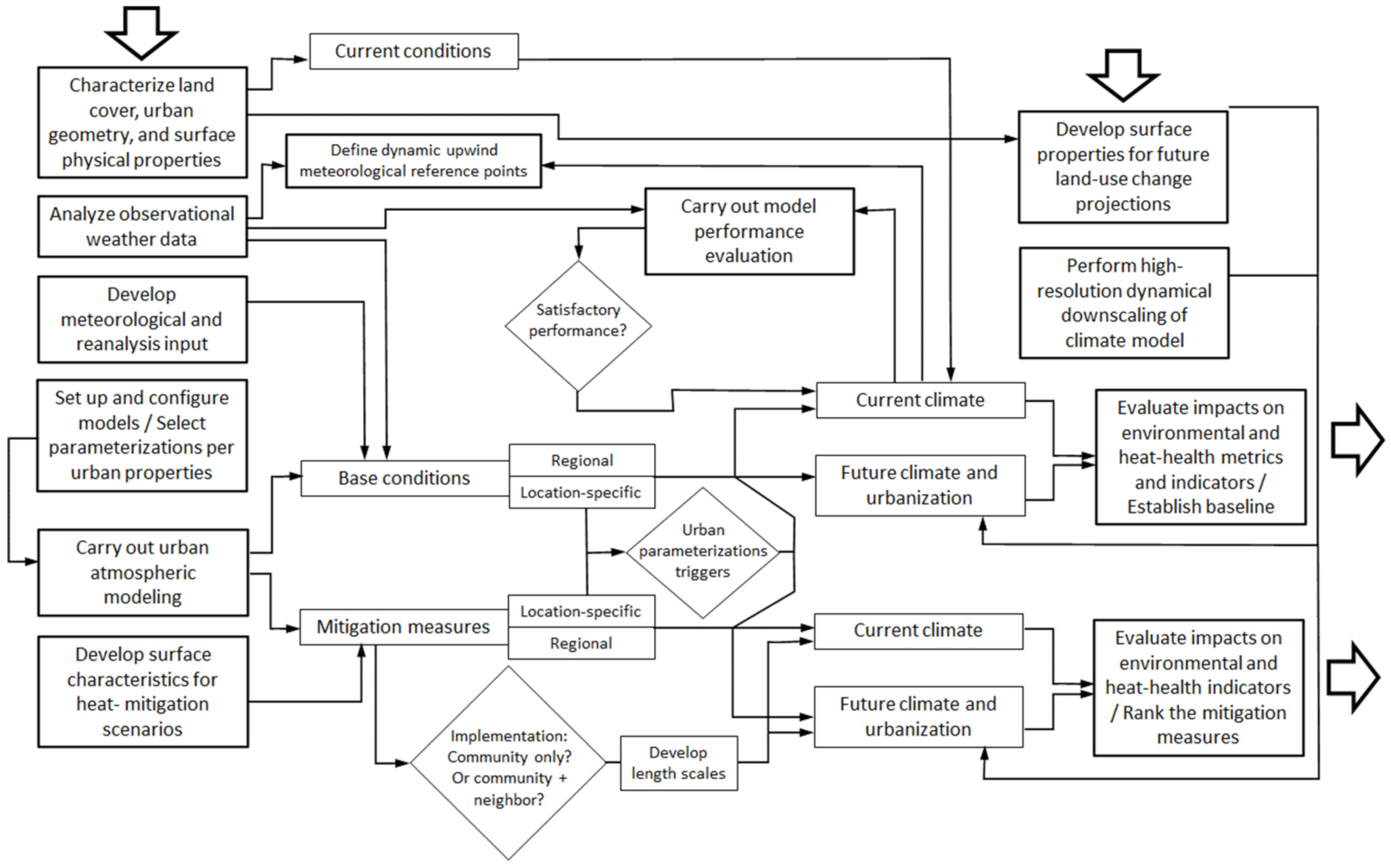
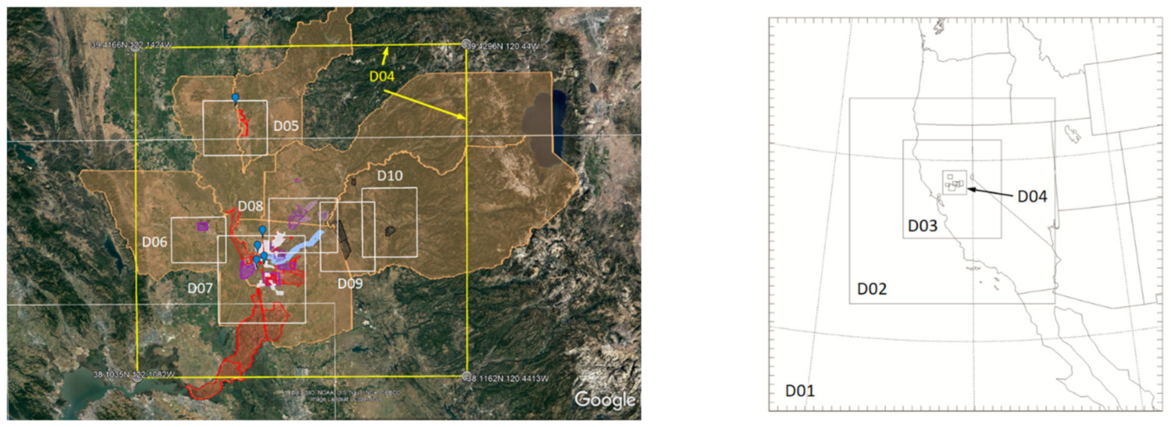
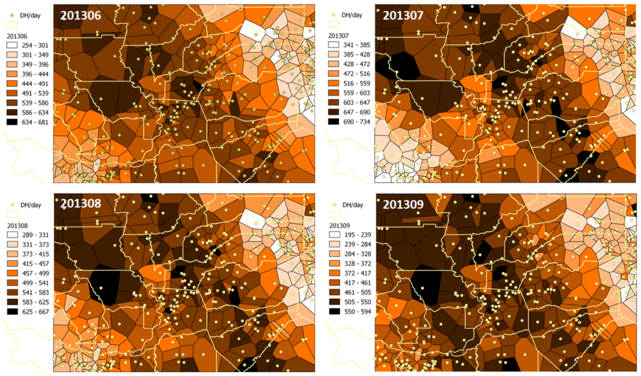
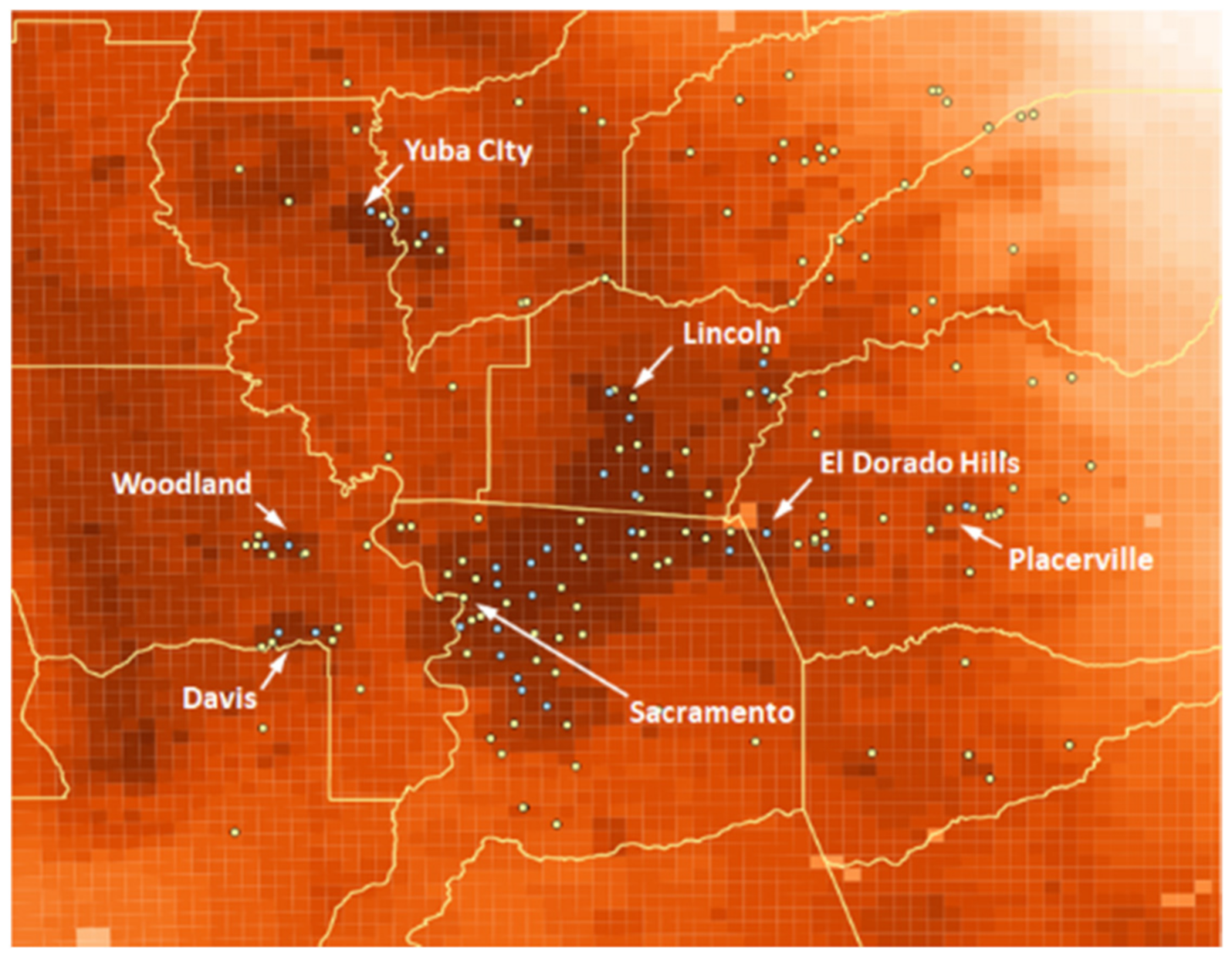
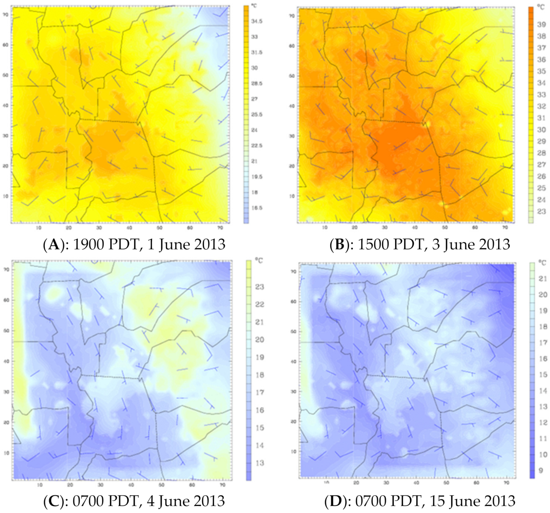
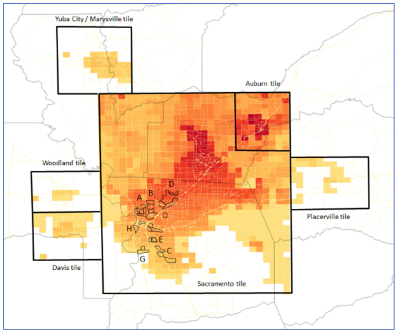
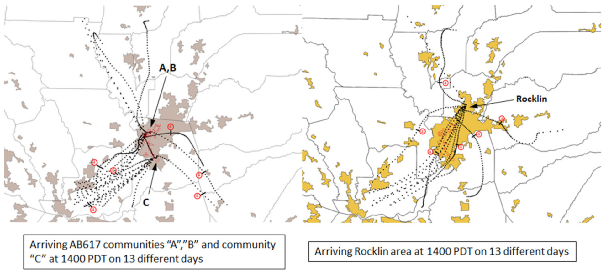
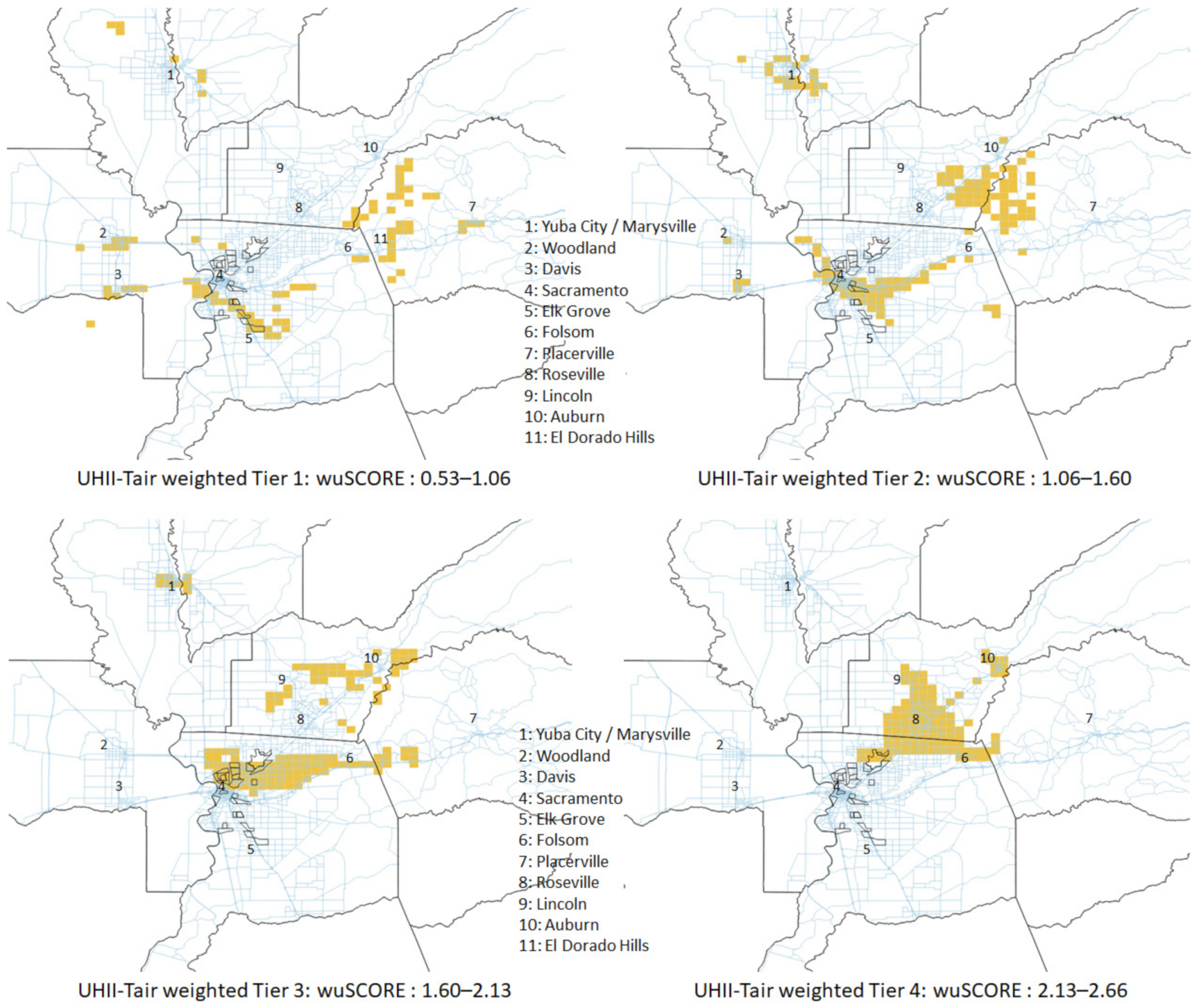
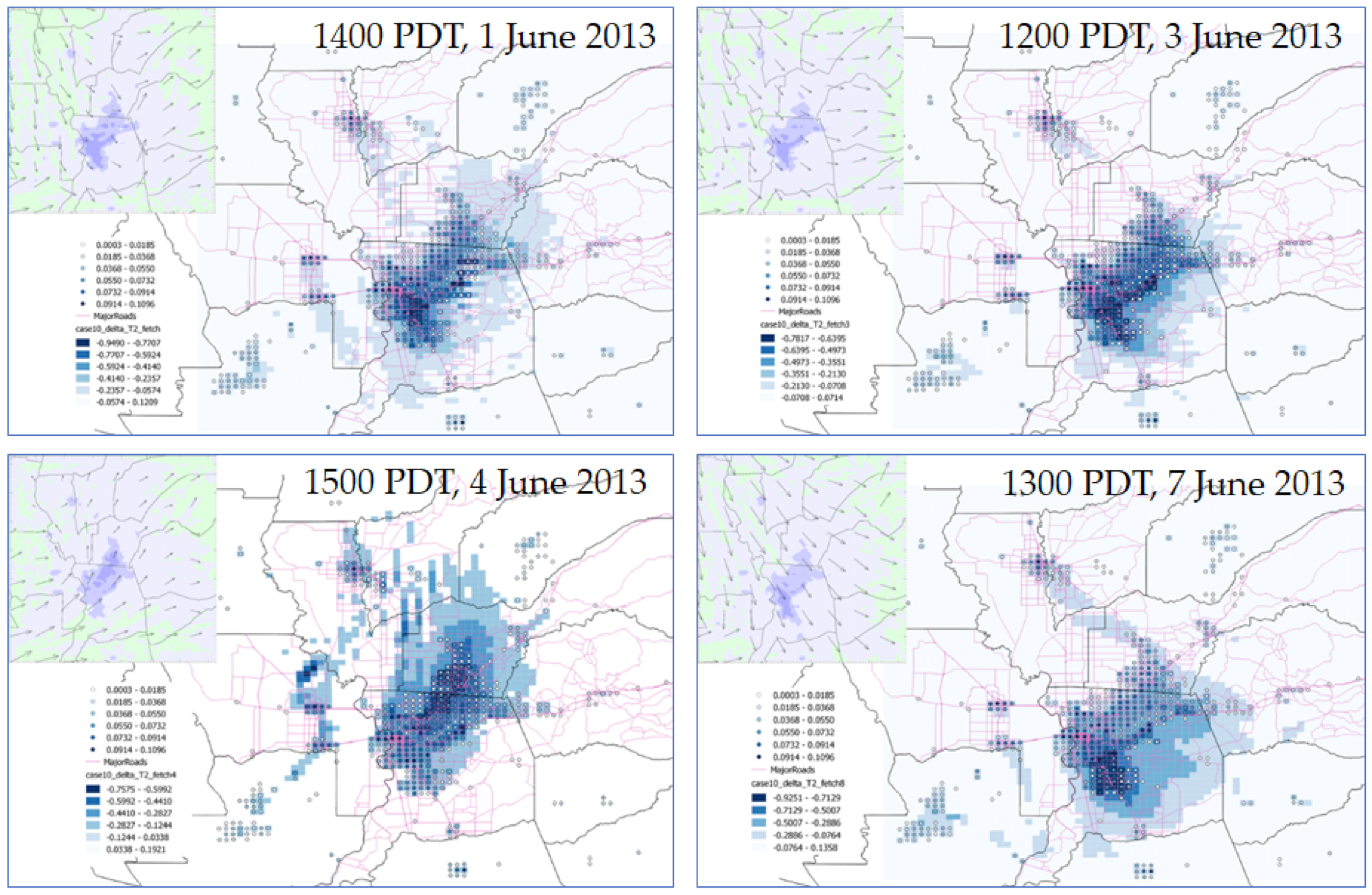
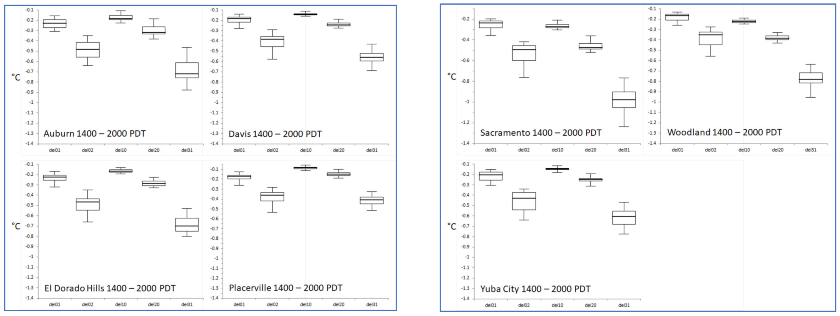
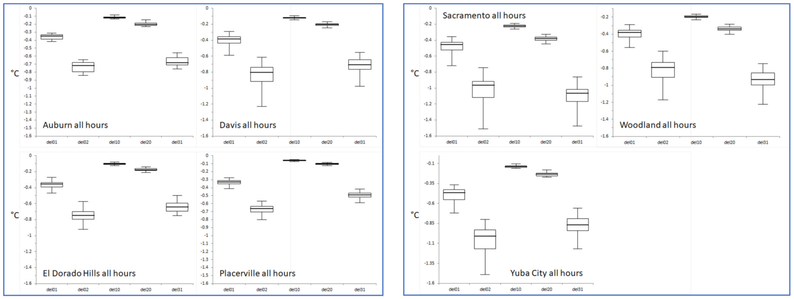
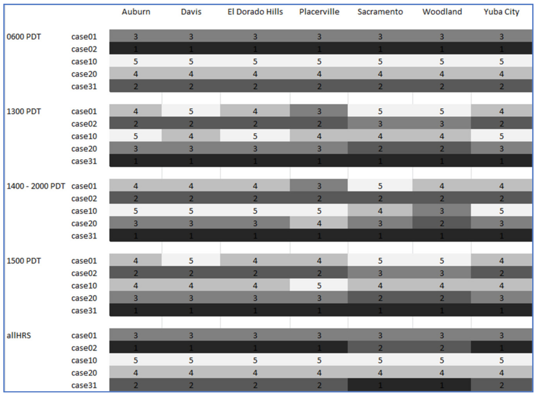
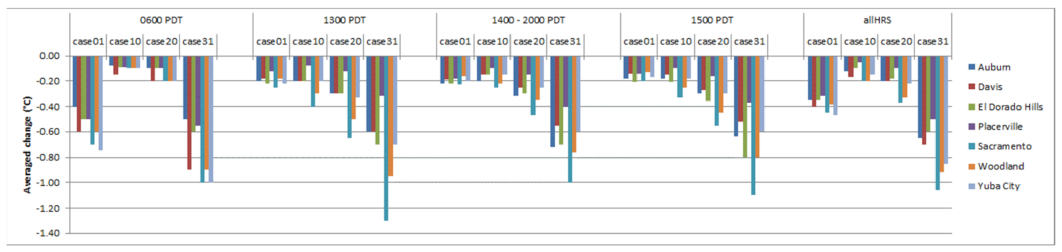
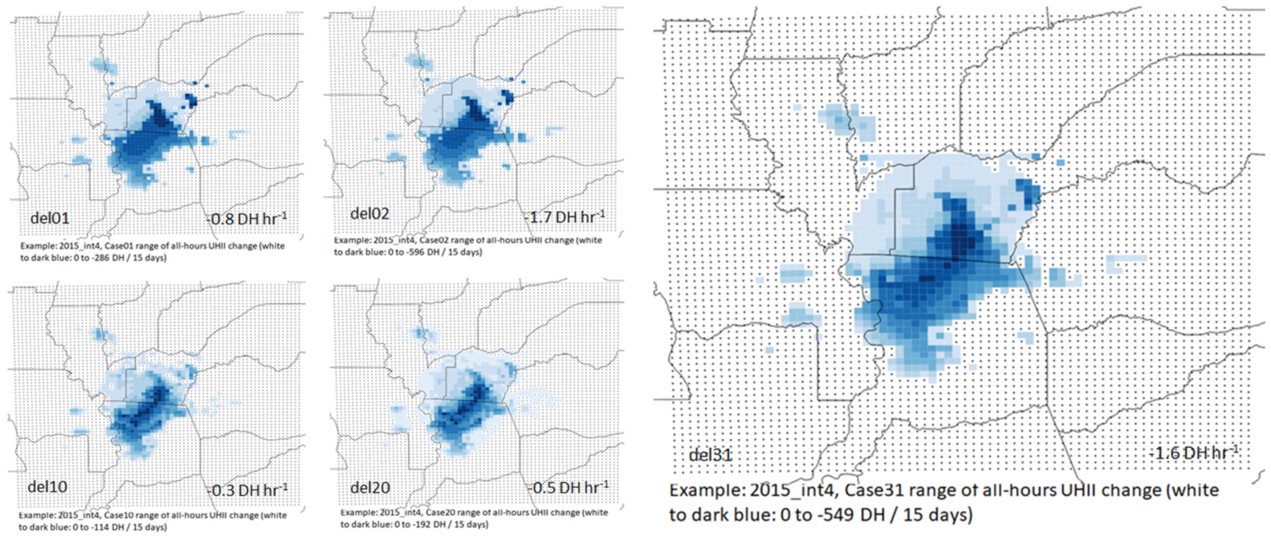
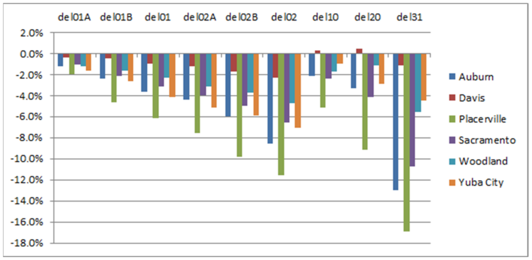
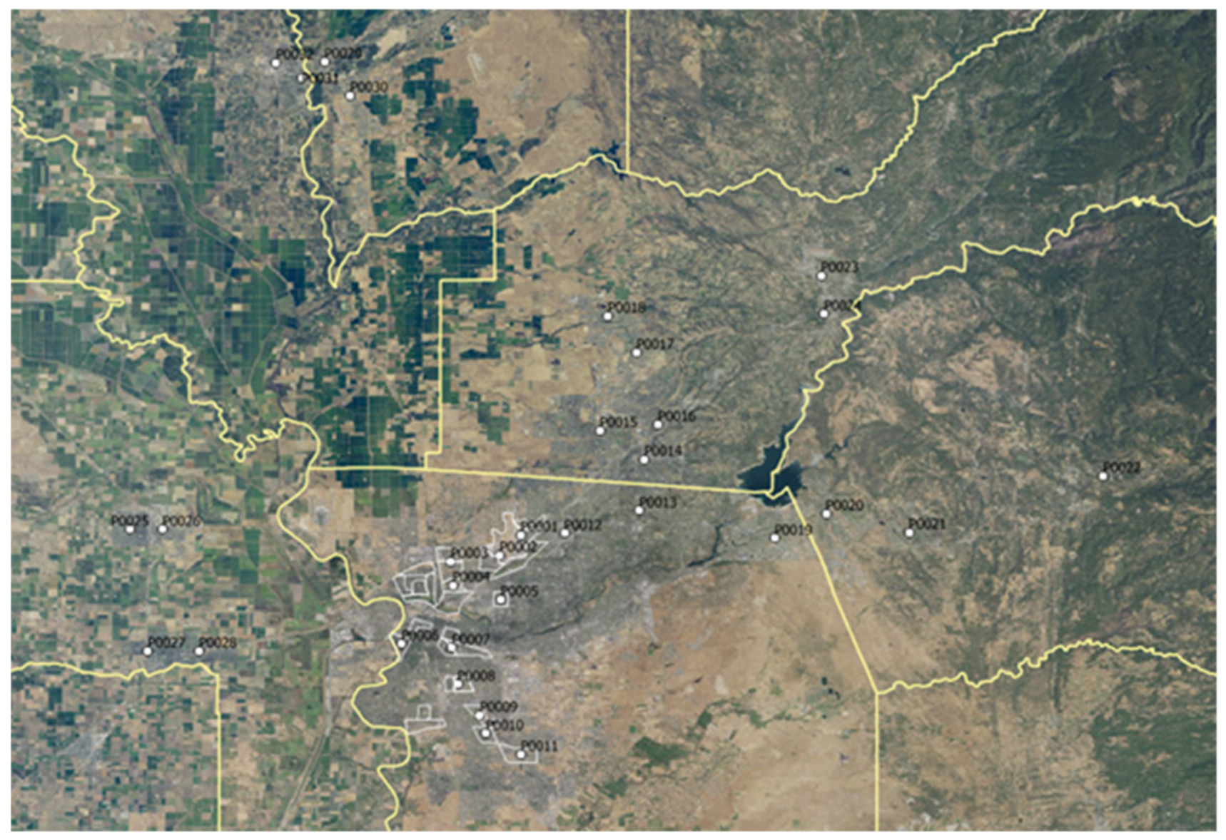
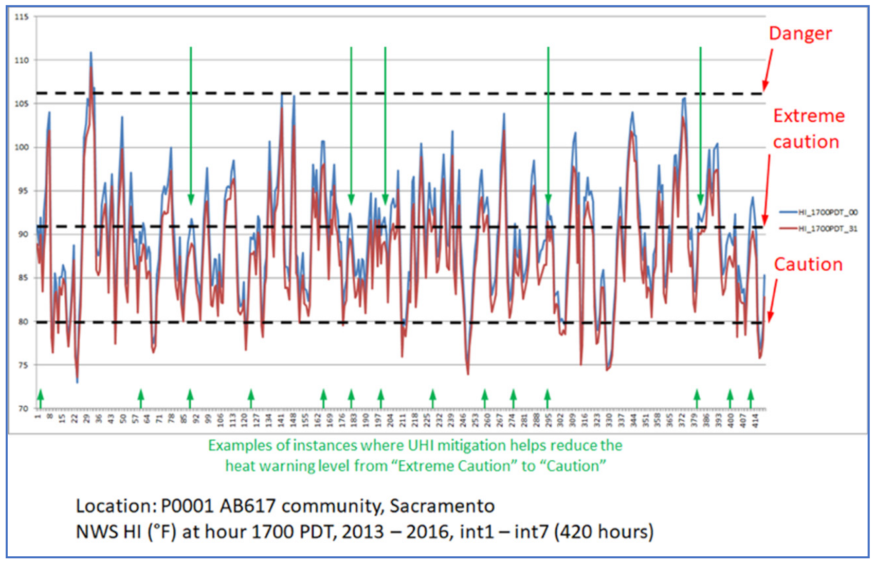
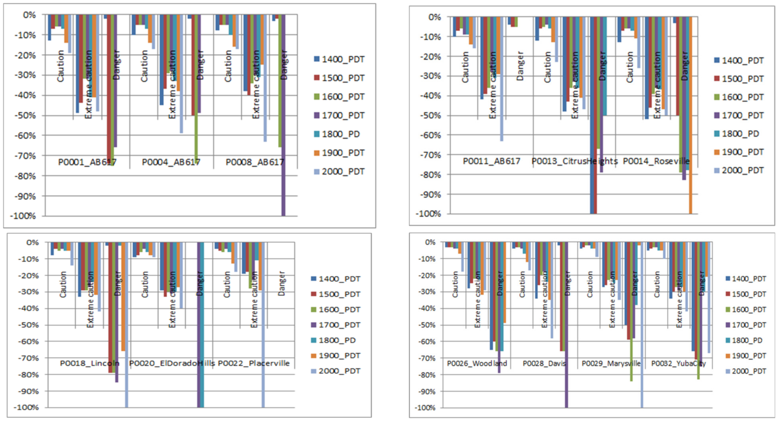
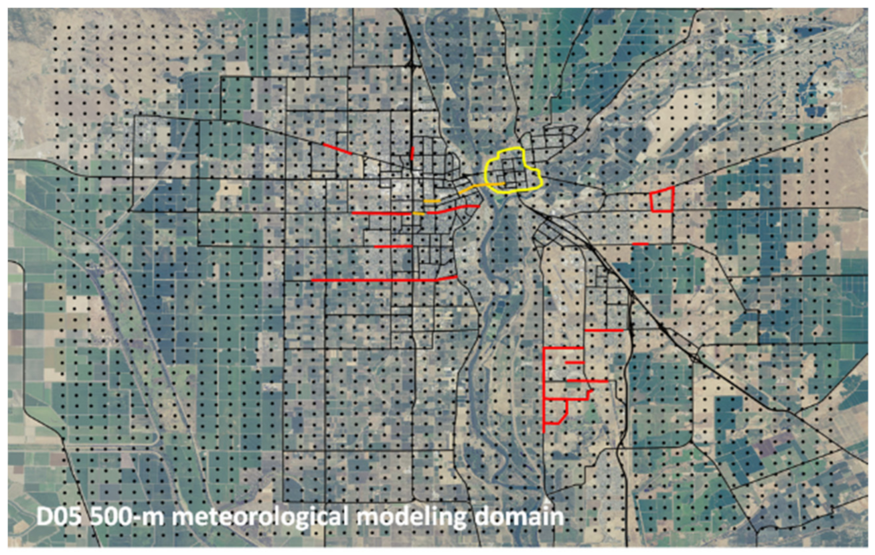
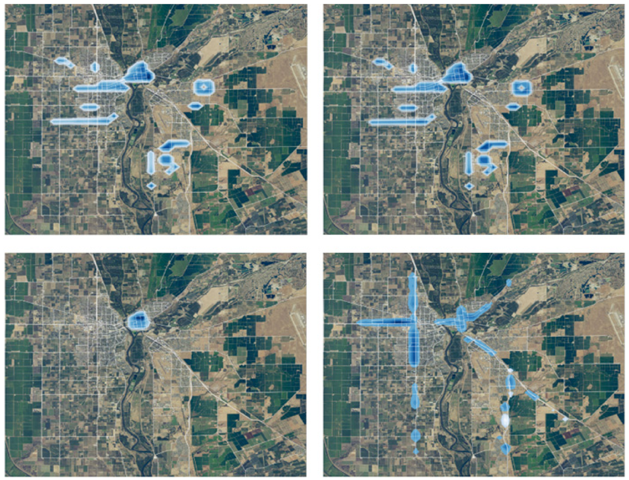
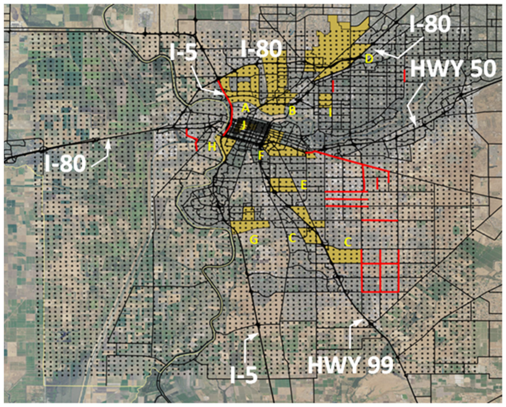
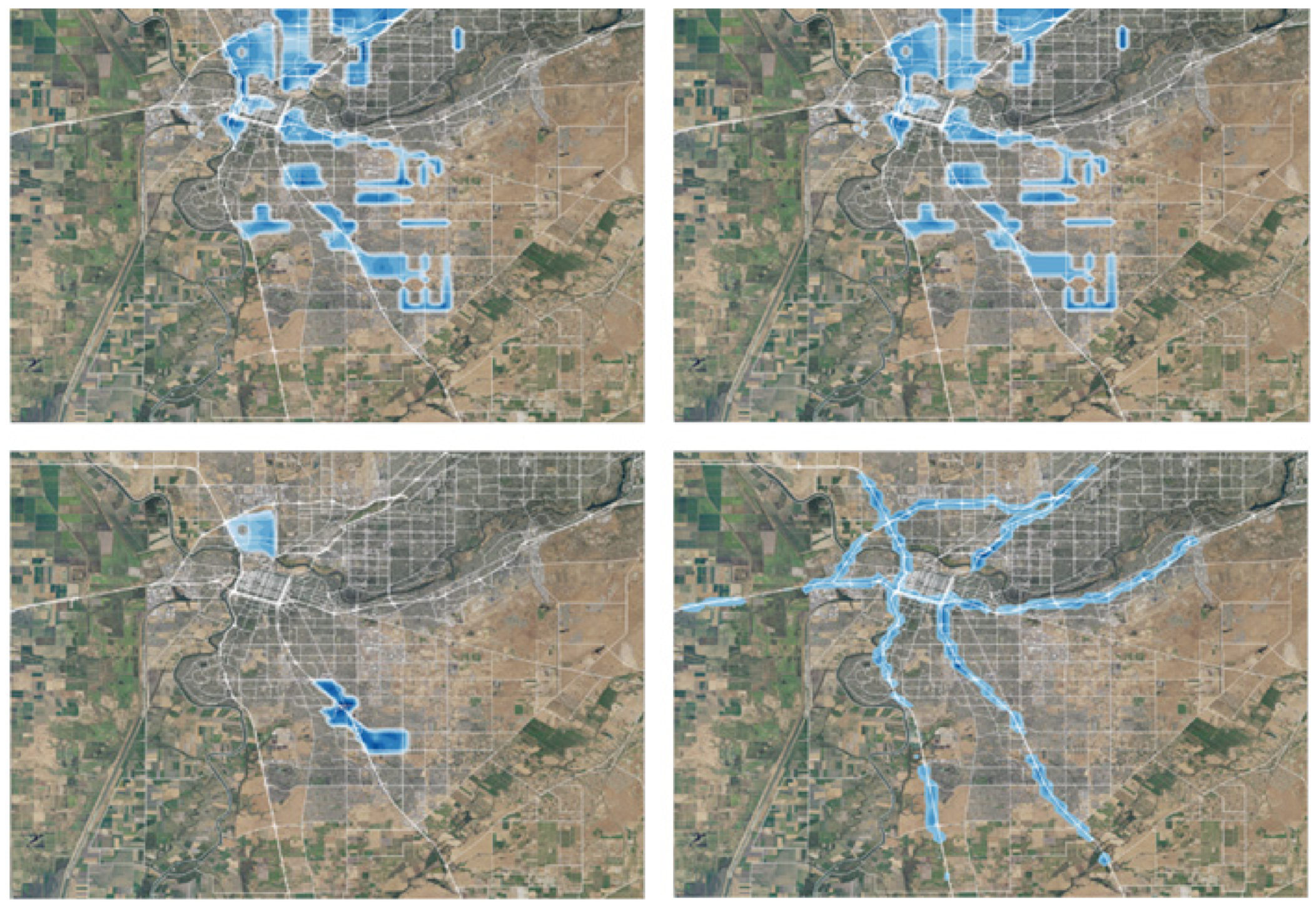
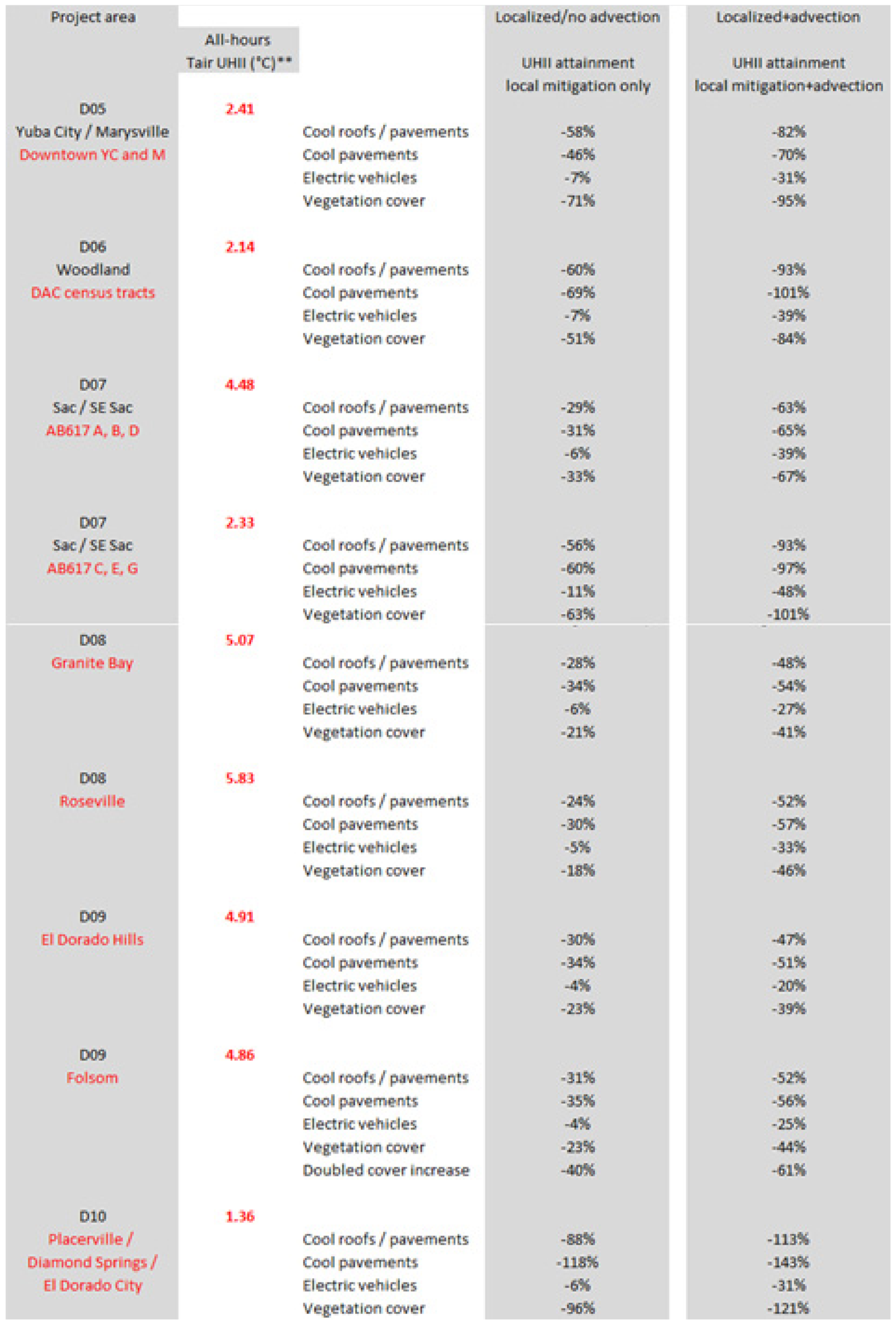
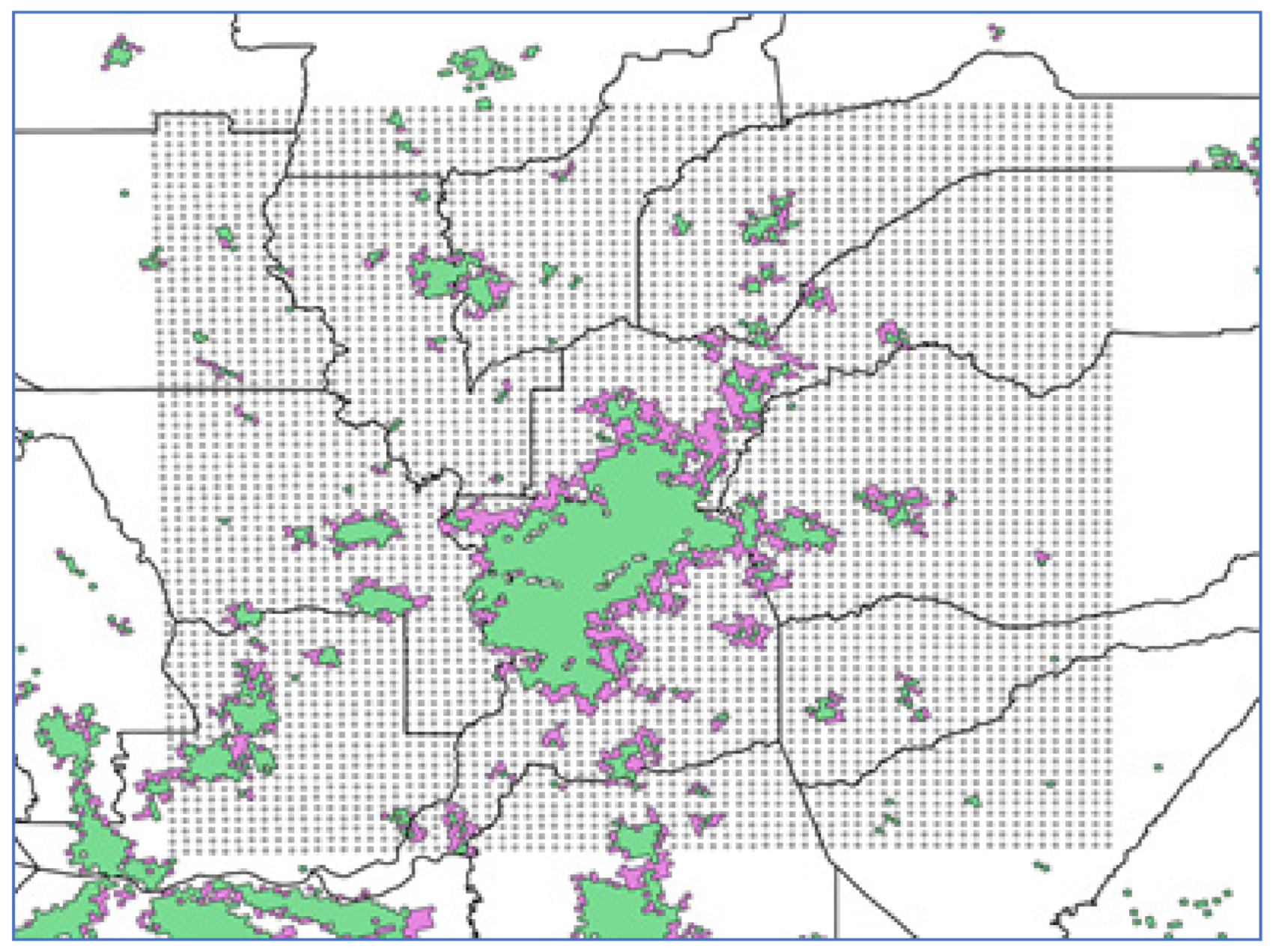
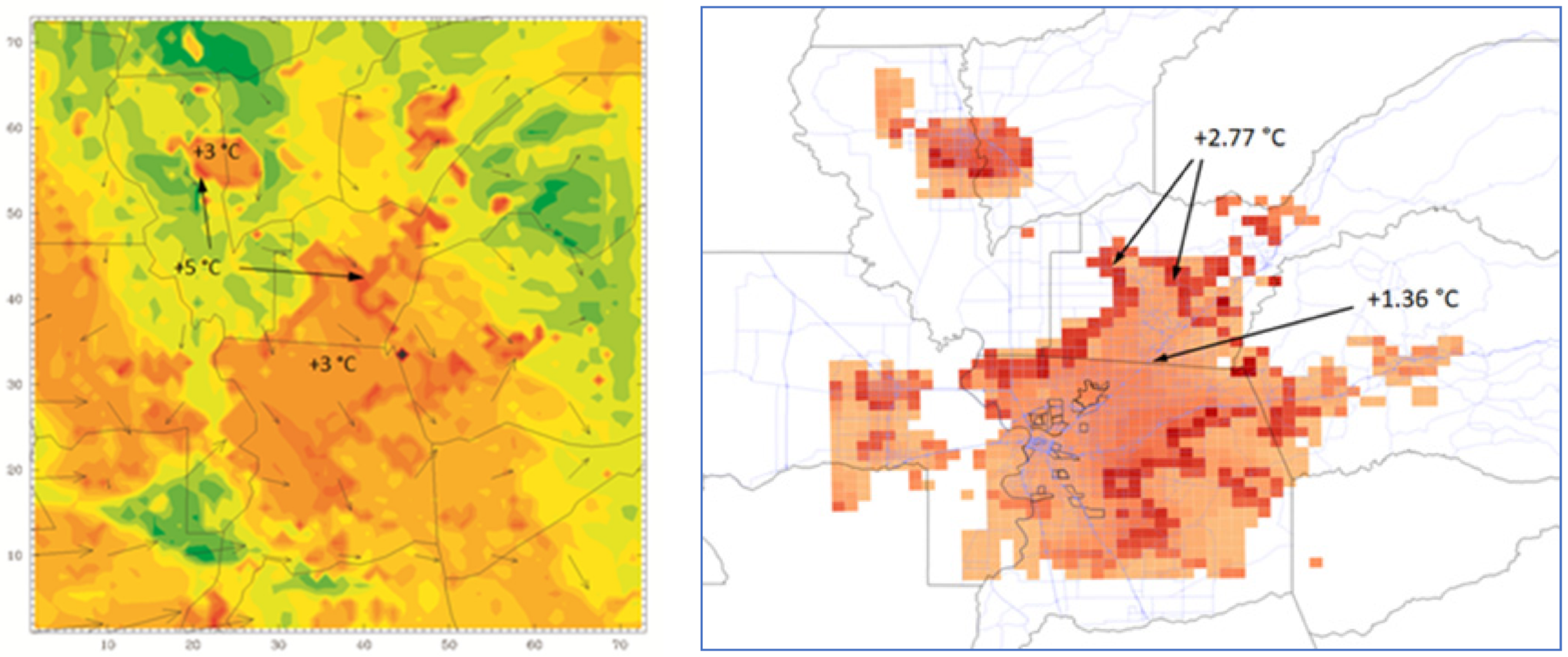
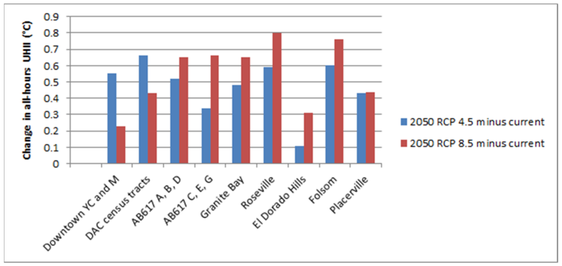
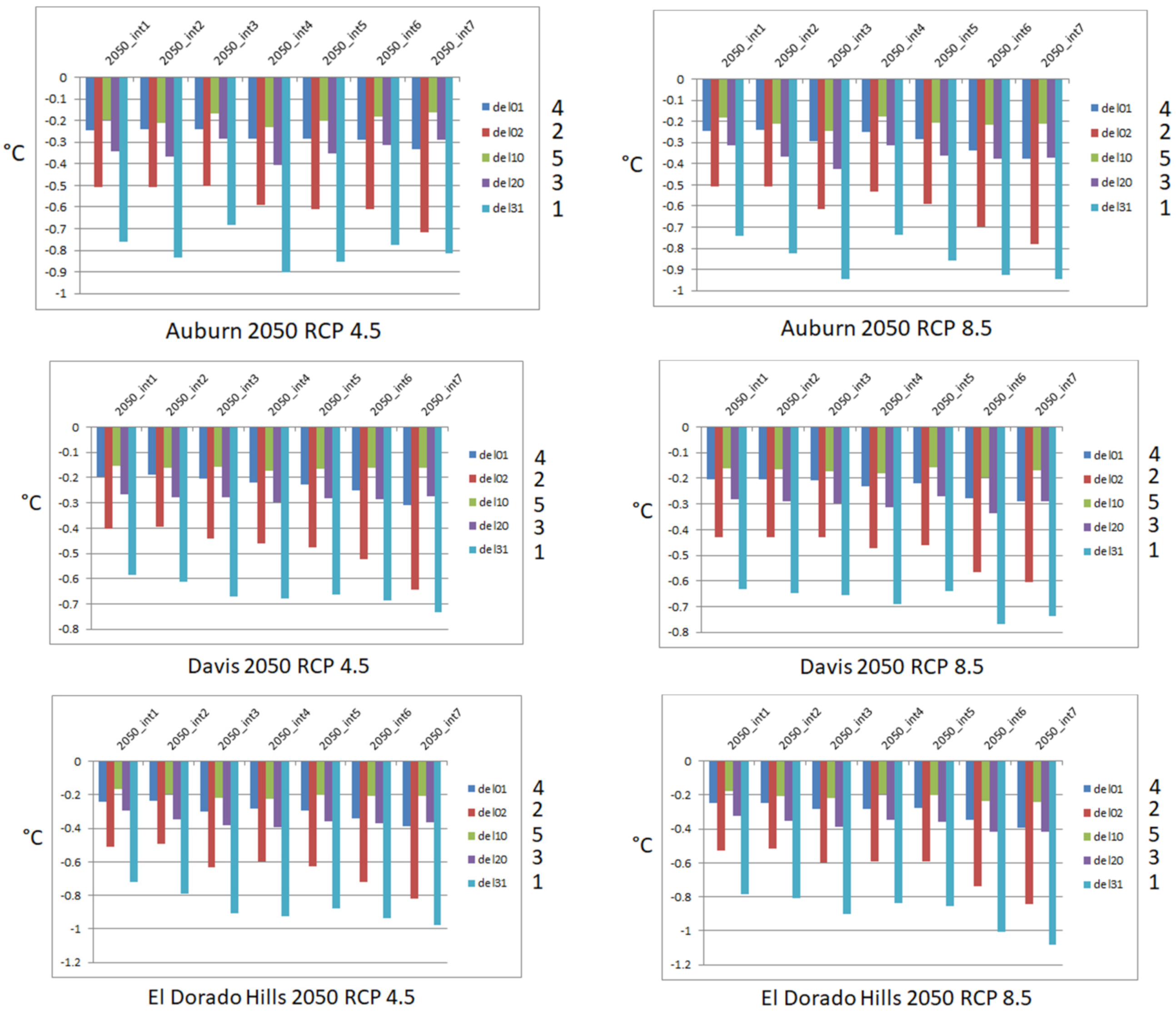
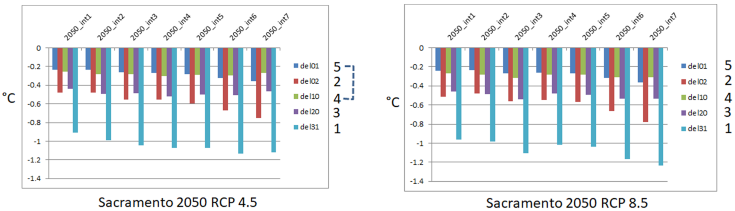
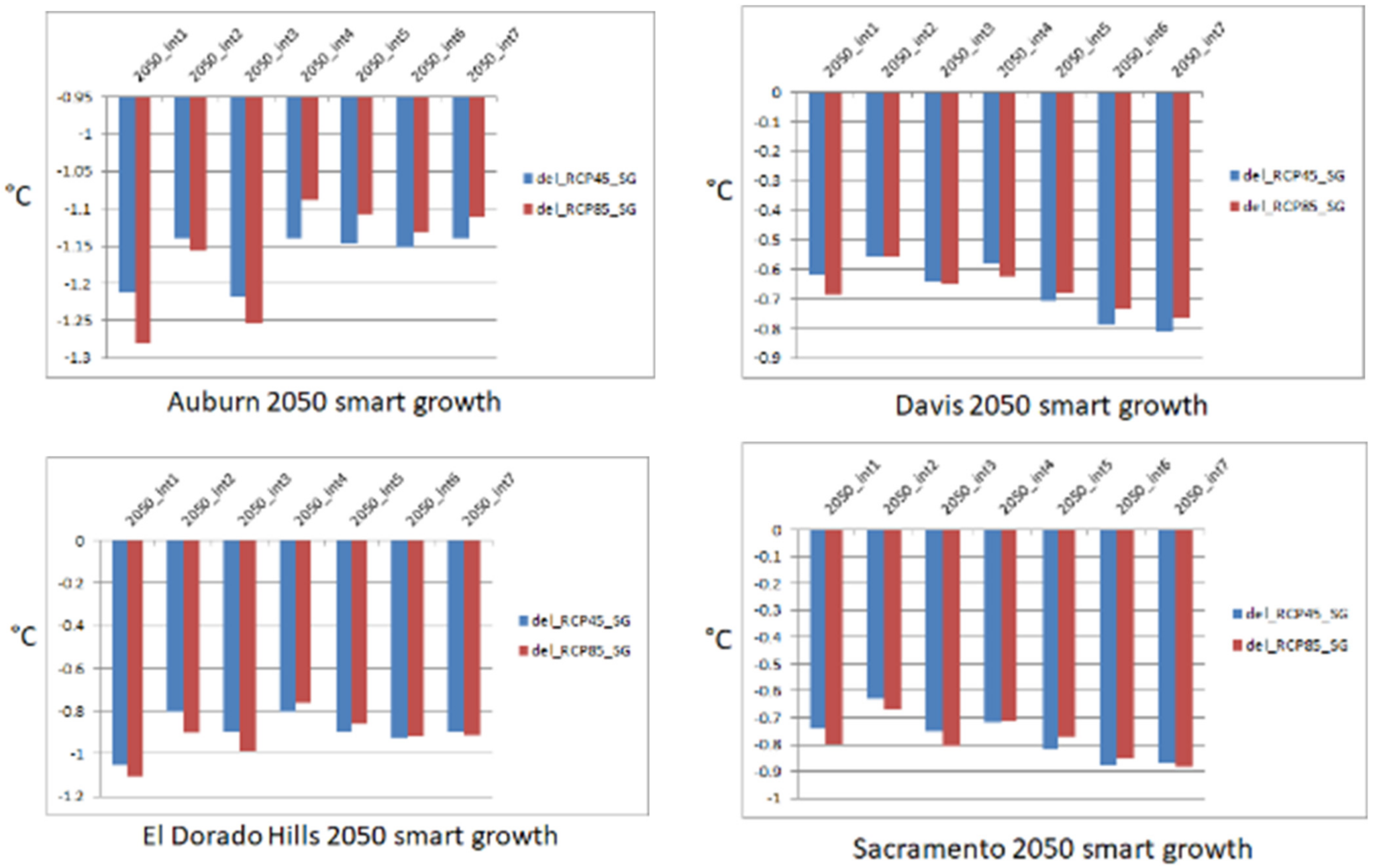
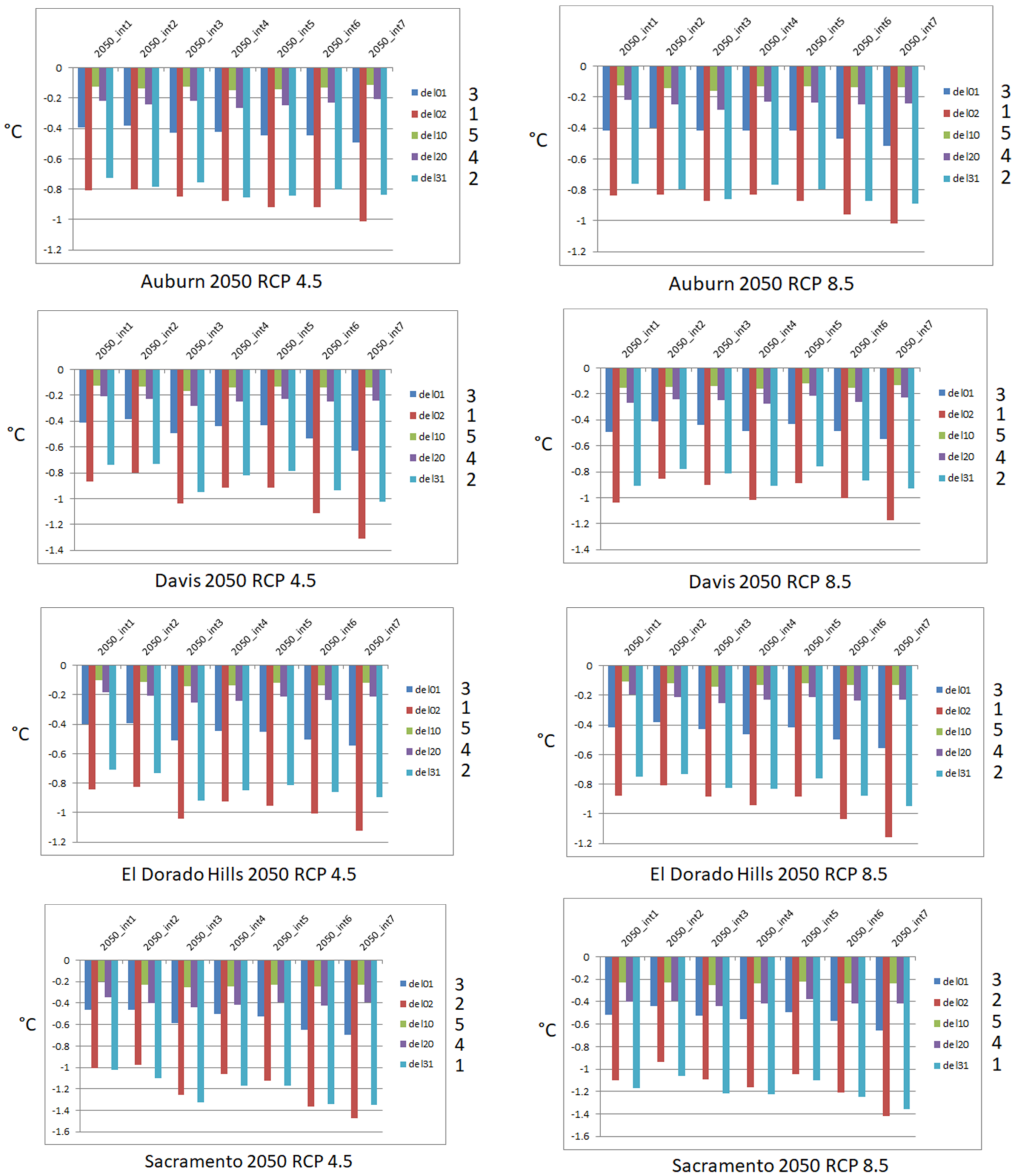
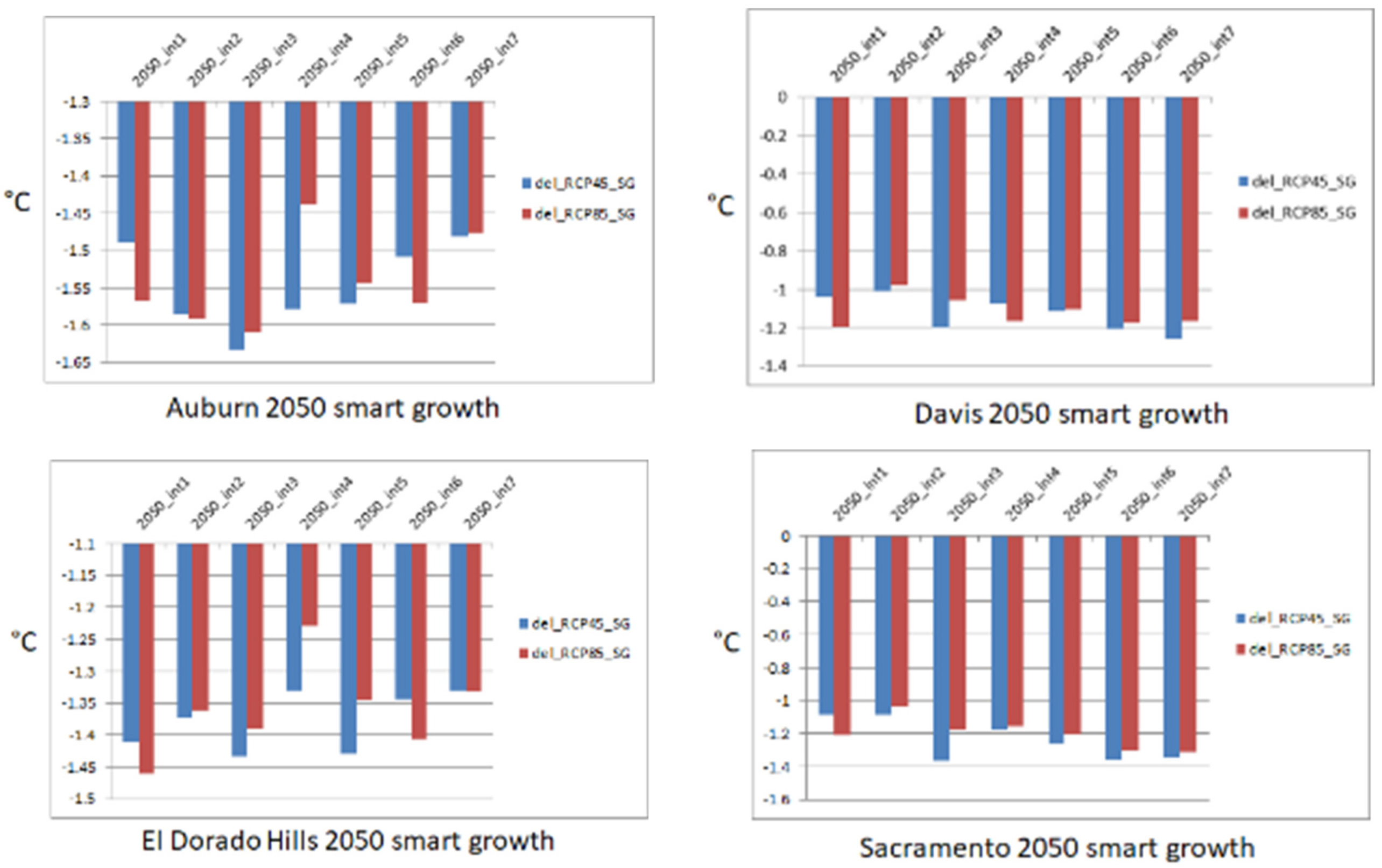
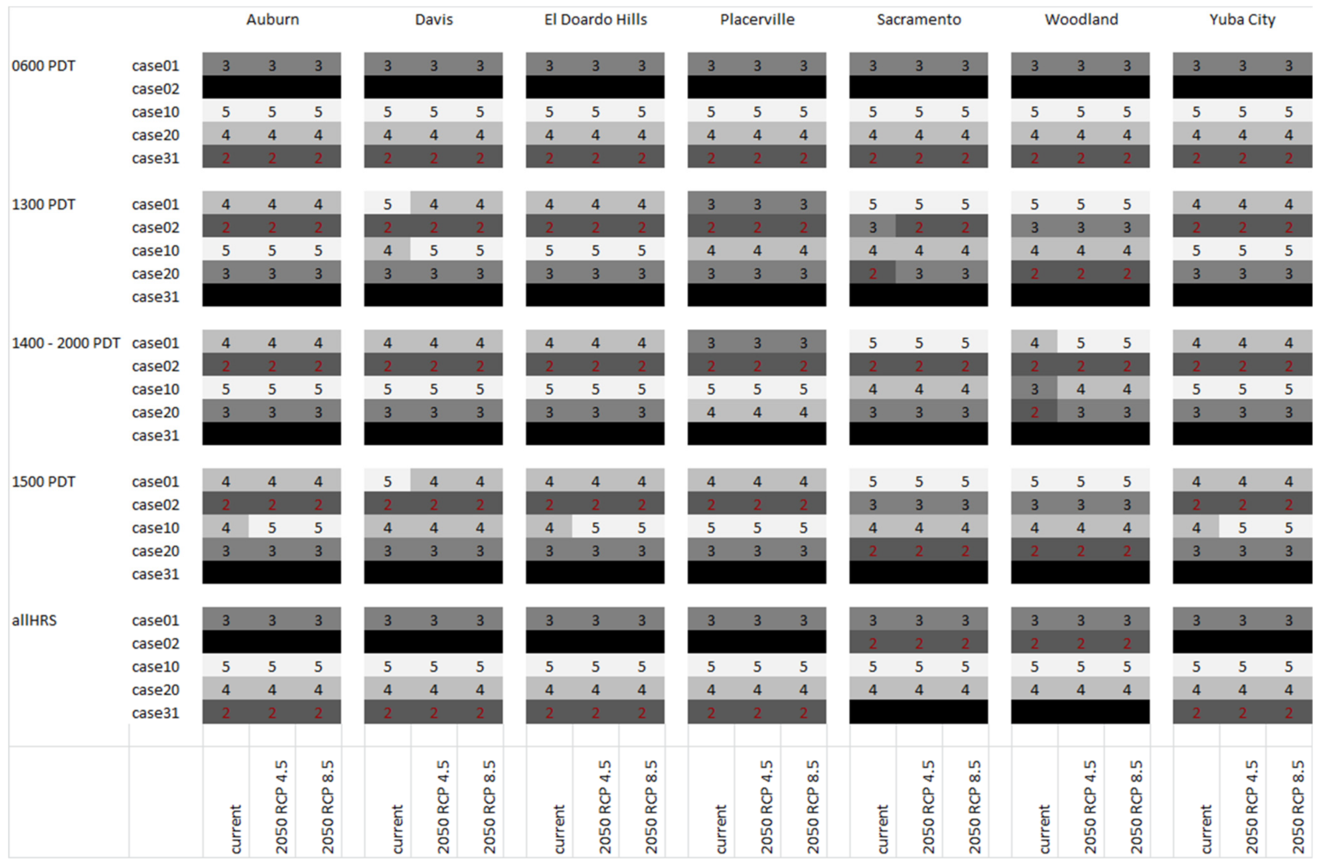
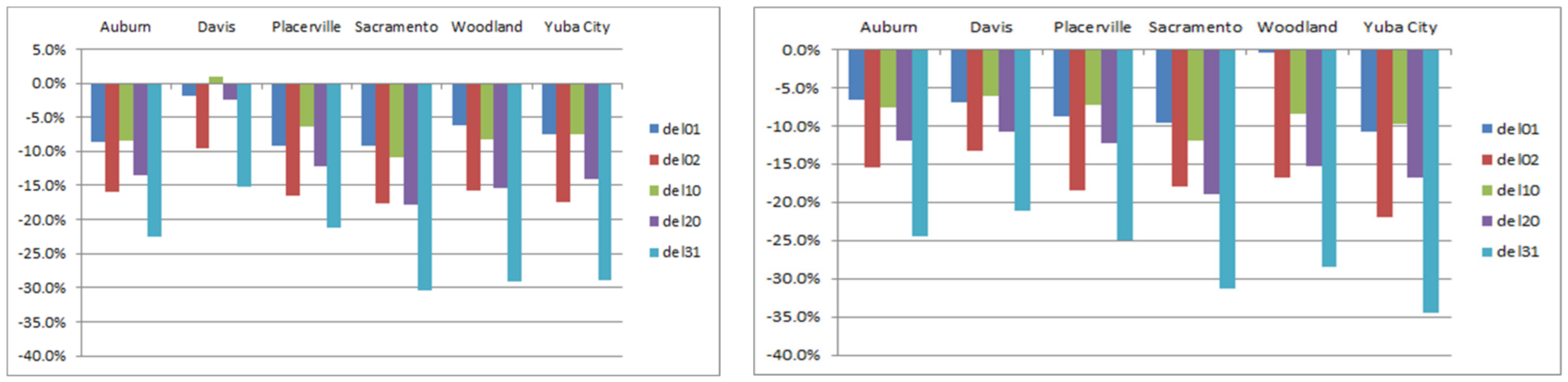
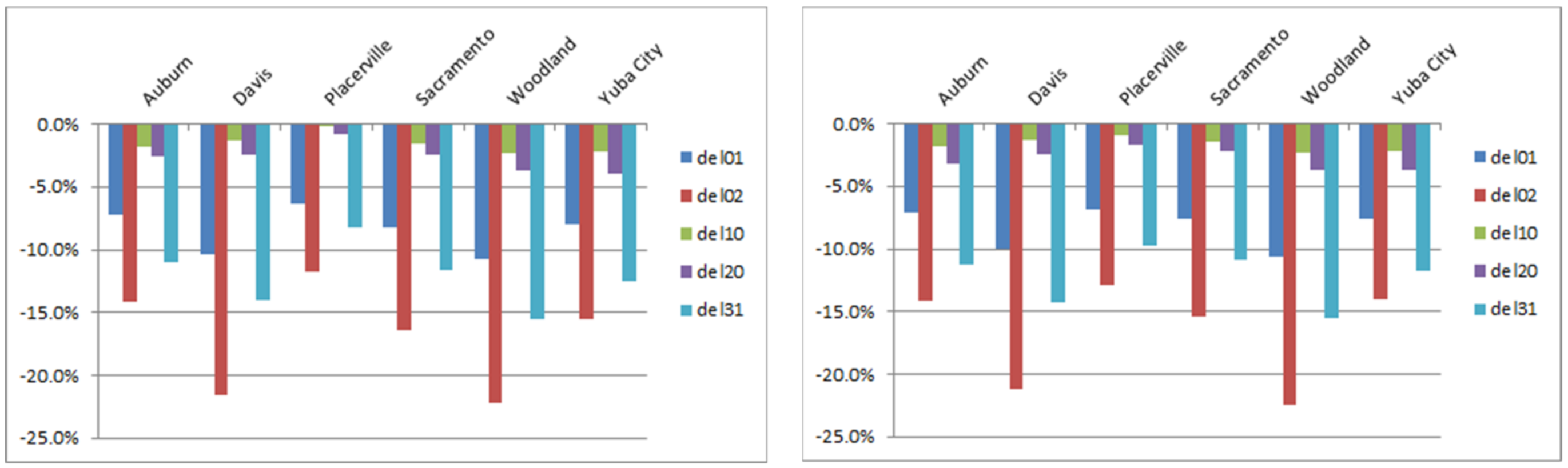
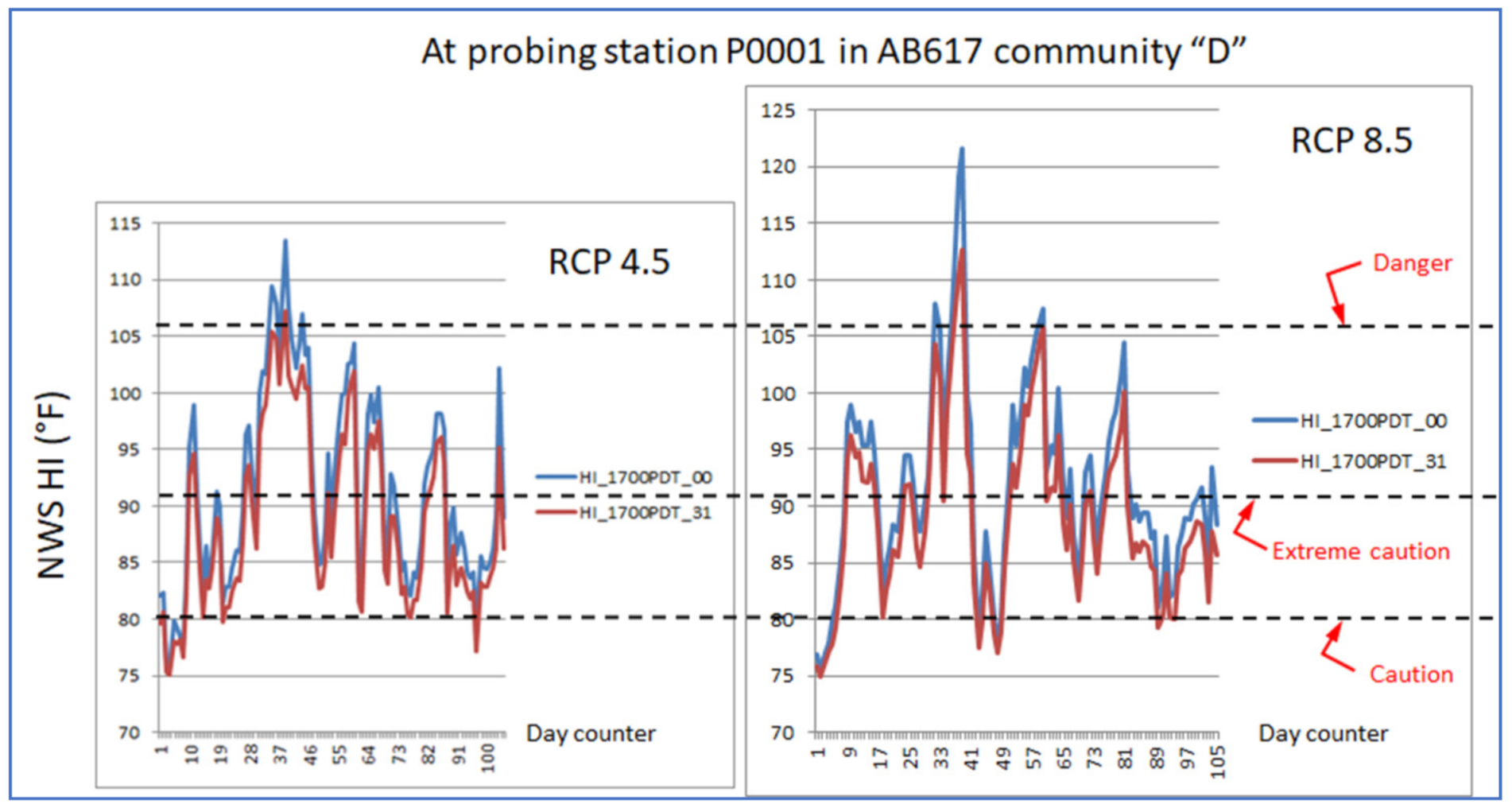
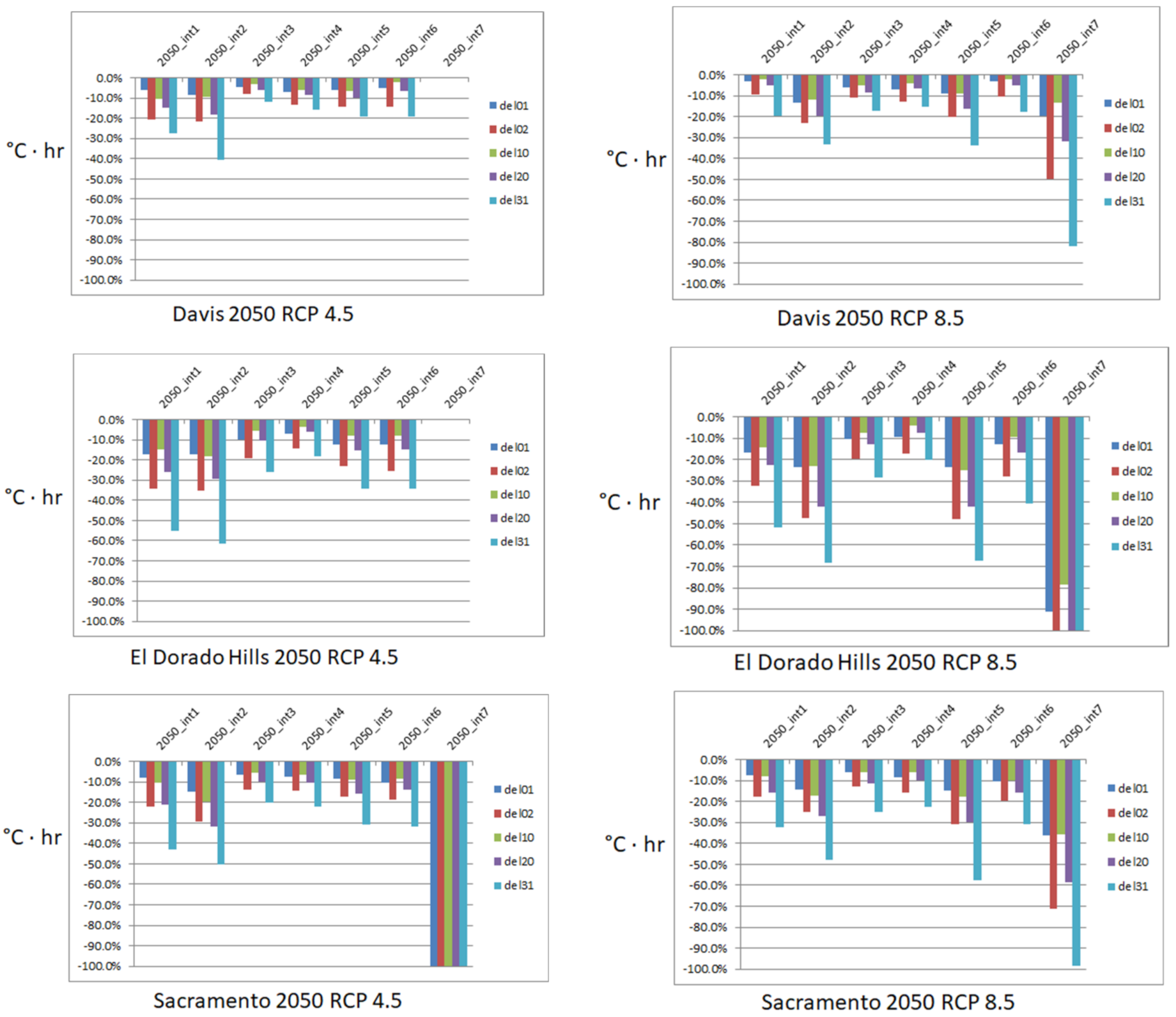
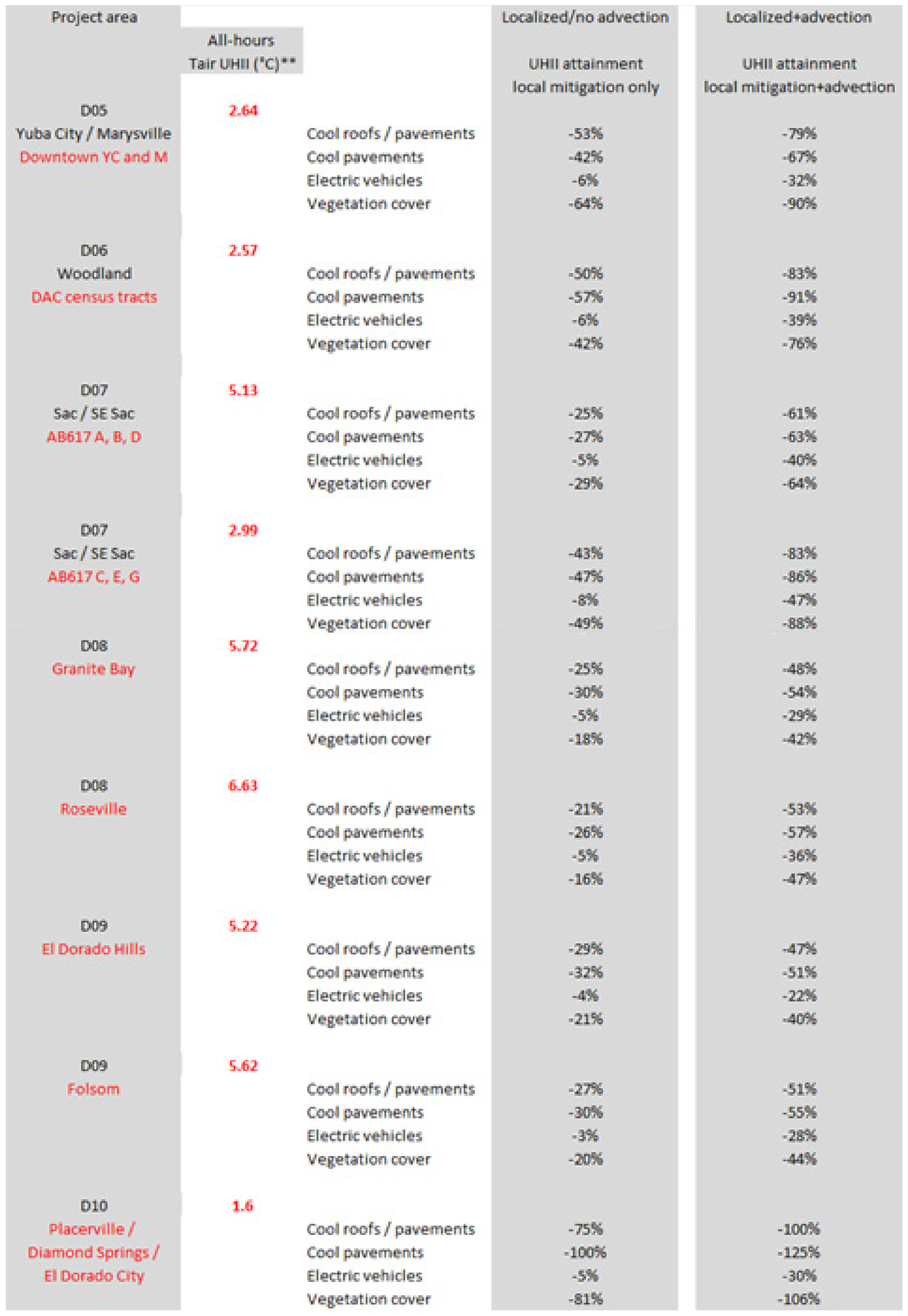
Table 1.
Upper bounds (maximum) for realistic increases in albedo.
| Case 10 (Max) | Case 20 (Max) | |
|---|---|---|
| Residential roof | +0.10 | +0.25 |
| Commercial roof | +0.20 | +0.30 |
| Roadway | +0.15 | +0.20 |
| Sidewalk/paved | +0.10 | +0.20 |
| Parking lots | +0.15 | +0.25 |
Table 2.
Exceedances above three NWS HI warning levels (1700 PDT averages over all intervals) in current climate at sample locations (P####) defined in Figure 18. All numbers are percentages.
Table 2.
Exceedances above three NWS HI warning levels (1700 PDT averages over all intervals) in current climate at sample locations (P####) defined in Figure 18. All numbers are percentages.
| HI Threshold | P0001 | P0004 | P0008 | P0011 | P0013 | P0014 | P0018 | P0020 | P0022 | P0026 | P0028 | |
|---|---|---|---|---|---|---|---|---|---|---|---|---|
| % of DH above threshold | >80 °F | 93.0 | 92.8 | 90.6 | 90.1 | 92.3 | 93.4 | 93.9 | 89.0 | 71.3 | 94.1 | 92.1 |
| >91 °F | 45.6 | 43.5 | 36.0 | 32.1 | 44.8 | 47.7 | 52.7 | 29.3 | 10.4 | 48.7 | 38.2 | |
| >106 °F | 0.9 | 0.6 | 0.3 | 0.0 | 1.4 | 1.7 | 2.0 | 29.3 | 10.4 | 48.7 | 38.2 | |
| % reduction in DH above thresholds | >80 °F | −5.8 | −5.0 | −5.2 | −9.4 | −4.9 | −6.1 | −4.7 | −4.8 | −4.8 | −4.2 | −4.8 |
| >91 °F | −31.9 | −28.6 | −30.5 | −28.0 | −33.5 | −36.2 | −27.0 | −31.9 | −23.3 | −22.3 | −18.7 | |
| >106 °F | −66.2 | −49.7 | −100.0 | N/A | −79.8 | −83.2 | −85.5 | −100.0 | N/A | −79.7 | −1.1 |
Table 3.
Number of consecutive days with NWS HI 105–110 °F in three time periods.
| Number of Days with NWS HI 105–110 °F | |||||||||
|---|---|---|---|---|---|---|---|---|---|
| 30 June–4 July 2013 | 30 June–1 July 2016 | 28 July–30 July 2016 | |||||||
| Probing Location | Heat Wave? | Base | Case 31 | Base | Case 31 | Base | Case 31 | ||
| P0001 AB617 (Sac) | yes | 5 | 1 | 0 | 0 | 2 | 0 | ||
| P0004 AB617 (Sac) | yes | 3 | 1 | 0 | 0 | 2 | 0 | ||
| P0008 AB617 (Sac) | 1 | 0 | 0 | 0 | 0 | 0 | |||
| P0011 AB617 (Sac) | 1 | 0 | 0 | 0 | 0 | 0 | |||
| P0013 Citrus Heights | yes | 5 | 1 | 1 | 0 | 1 | 0 | ||
| P0014 Roseville | yes | 5 | 2 | 1 | 0 | 2 | 0 | ||
| P0018 Lincoln | yes | 4 | 3 | 1 | 0 | 2 | 0 | ||
| P0020 El Dorado Hills | 1 | 0 | 0 | 0 | 0 | 0 | |||
| P0022 Placerville | 0 | 0 | 0 | 0 | 0 | 0 | |||
| P0026 Woodland | yes | 3 | 0 | 0 | 0 | 0 | 0 | ||
| P0028 Davis | yes | 4 | 0 | 0 | 0 | 0 | 0 | ||
| P0029 Marysville | yes | 4 | 4 | 2 | 0 | 3 | 2 | ||
| P0032 Yuba City | yes | 4 | 4 | 2 | 0 | 3 | 1 | ||
Table 4.
Changes in temperature as area-wide and time averages per given hour or range of hours (averaged over three intervals defined in Section 5.11.1) for the Yuba City/Marysville area. In canopy cover and electrification scenarios, a better indicator is to average Tair and Tsfc (see text for explanation).
| D05 Marysville/Yuba City | |||||
|---|---|---|---|---|---|
| Case A (Avg. Change in °C) | Case B (Avg. Change in °C) | Case QF (Avg. Change in °C) | |||
| 0600 PDT | Tair | Roofs and pavements | −0.24 | −0.34 | |
| Roadways | −0.17 | ||||
| Tsfc | Roofs and pavements | −0.46 | −2.23 | ||
| Roadways | −0.35 | ||||
| 0700 PDT | Tair | −0.05 | |||
| Tsfc | −0.18 | ||||
| 1300 PDT | Tair | Roofs and pavements | −3.07 | −0.43 | |
| Roadways | −2.09 | ||||
| Tsfc | Roofs and pavements | −8.28 | −2.56 | ||
| Roadways | −5.53 | ||||
| 1500 PDT | Tair | Roofs and pavements | −2.68 | −0.40 | |
| Roadways | −2.46 | ||||
| Tsfc | Roofs and pavements | −7.45 | −2.50 | ||
| Roadways | −6.33 | ||||
| 1700 PDT | Tair | −0.06 | |||
| Tsfc | −0.37 | ||||
| All hours | Tair | Roofs and pavements | −1.38 | −0.49 | −0.04 |
| Roadways | −1.11 | ||||
| Tsfc | Roofs and pavements | −3.57 | −2.87 | −0.24 | |
| Roadways | −2.68 | ||||
Table 5.
Changes in temperature as area-wide and time averages per given hour or range of hours (averaged over three intervals defined in Section 5.11.1) for the Sacramento area. In canopy cover and electrification scenarios, a better indicator is to average Tair and Tsfc (see text for explanation).
| D07 Sacramento | |||||
|---|---|---|---|---|---|
| Case A (Avg. Change in °C) | Case B (Avg. Change in °C) | Case QF (Avg Change in °C) | |||
| 0600 PDT | Tair | Roofs and pavements | −0.25 | −0.39 | |
| Roadways | −0.24 | ||||
| Tsfc | Roofs and pavements | −0.44 | −2.25 | ||
| Roadways | −0.45 | ||||
| 0700 PDT | Tair | −0.04 | |||
| Tsfc | −0.39 | ||||
| 1300 PDT | Tair | Roofs and pavements | −2.79 | −0.14 | |
| Roadways | −3.14 | ||||
| Tsfc | Roofs and pavements | −6.98 | −1.52 | ||
| Roadways | −7.90 | ||||
| 1500 PDT | Tair | Roofs and pavements | −2.67 | −0.21 | |
| Roadways | −2.90 | ||||
| Tsfc | Roofs and pavements | −6.70 | −2.03 | ||
| Roadways | −7.39 | ||||
| 1700 PDT | Tair | −0.11 | |||
| Tsfc | −0.69 | ||||
| All hours | Tair | Roofs and pavements | −1.31 | −0.41 | −0.07 |
| Roadways | −1.45 | ||||
| Tsfc | Roofs and pavements | −3.08 | −2.54 | −0.43 | |
| Roadways | −3.46 | ||||
Table 6.
All-hours UHII and changes (temperature equivalent in °C) at sample locations.
| Domain | Area | All-Hours UHII (Temperature Equivalent °C) | ||
|---|---|---|---|---|
| 2013–2016 | 2050 RCP 4.5 | 2050 RCP 8.5 | ||
| D05 | Yuba City/Marysville | 2.41 | 2.96 | 2.64 |
| D06 | Woodland | 2.14 | 2.80 | 2.57 |
| D07 | Sacramento, communities A, B, D | 4.48 | 5.00 | 5.13 |
| D07 | Sacramento, communities C, E, G | 2.33 | 2.67 | 2.99 |
| D08 | Granite Bay | 5.07 | 5.55 | 5.72 |
| D08 | Roseville | 5.83 | 6.42 | 6.63 |
| D09 | El Dorado Hills | 4.91 | 5.02 | 5.22 |
| D09 | Folsom | 4.86 | 5.46 | 5.62 |
| D10 | Placerville | 1.36 | 1.59 | 1.60 |
Table 7.
NWS HI at 1700 PDT: exceedances above thresholds and reduction from case31. All numbers are percentages. (These are sample locations P0001–P0020.
Table 7.
NWS HI at 1700 PDT: exceedances above thresholds and reduction from case31. All numbers are percentages. (These are sample locations P0001–P0020.
| P0001 AB617 | HI Threshold | 2013–2016 | 2050 RCP 4.5 | 2050 RCP 8.5 |
| % of DH above threshold | >80 °F | 93.0 | 94.3 | 93.5 |
| >91 °F | 45.6 | 49.8 | 51.2 | |
| >106 °F | 0.9 | 6.8 | 8.1 | |
| % reduction in DH above thresholds | >80 °F | −5.2 | −4.7 | −7.6 |
| >91 °F | −31.9% | −20.2 | −23.4 | |
| >106 °F | −66.2 | −83.6 | −57.7 | |
| P0004 AB617 | HI threshold | 2013–2016 | 2050 RCP 4.5 | 2050 RCP 8.5 |
| % of DH above threshold | >80 °F | 92.8 | 94.3 | 92.7 |
| >91 °F | 43.5 | 48.9 | 49.4 | |
| >106 °F | 0.6 | 5.7 | 8.1 | |
| % reduction in DH above thresholds | >80 °F | −5.0 | −5.2 | −7.1 |
| >91 °F | −28.6 | −22.3 | −27.8 | |
| >106 °F | −49.7 | −80.4 | −57.8 | |
| P0008 AB617 | HI threshold | 2013–2016 | 2050 RCP 4.5 | 2050 RCP 8.5 |
| % of DH above threshold | >80 °F | 90.6 | 92.6 | 90.1 |
| >91 °F | 36.0 | 43.2 | 43.6 | |
| >106 °F | 0.3 | 4.6 | 9.2 | |
| % reduction in DH above thresholds | −5.2% | −9.6 | −4.1 | −5.2 |
| −30.5% | −13.8 | −33.2 | −30.5 | |
| −100.0% | −100.0 | −100.0 | −100.0 | |
| P0014 Roseville | HI threshold | 2013–2016 | 2050 RCP 4.5 | 2050 RCP 8.5 |
| % of DH above threshold | >80 °F | 93.4 | 94.3 | 95.2 |
| >91 °F | 47.7 | 49.6 | 52.2 | |
| >106 °F | 1.7 | 7.9 | 7.1 | |
| % reduction in DH above thresholds | −5.2% | −6.1 | −4.1 | −8.7 |
| −30.5% | −36.2 | −20.3 | −23.4 | |
| −100.0% | −83.2 | −100.0 | −51.1 | |
| P0018 Lincoln | HI threshold | 2013–2016 | 2050 RCP 4.5 | 2050 RCP 8.5 |
| % of DH above threshold | >80 °F | 93.9 | 95.1 | 95.2 |
| >91 °F | 52.7 | 48.4 | 52.1 | |
| >106 °F | 2.0 | 4.5 | 6.1 | |
| % reduction in DH above thresholds | −5.2% | −4.7 | −2.9 | −5.8 |
| −30.5% | −27.0 | −15.8 | −15.0 | |
| −100.0% | −85.5 | −75.3 | −40.2 | |
| P0020 ED Hills | HI threshold | 2013–2016 | 2050 RCP 4.5 | 2050 RCP 8.5 |
| % of DH above threshold | >80 °F | 89.0 | 93.4 | 90.9 |
| >91 °F | 29.3 | 37.8 | 38.5 | |
| >106 °F | 0.3 | 1.1 | 3.7 | |
| % reduction in DH above thresholds | −5.2% | −4.8 | −8.5 | −7.1 |
| −30.5% | −31.9 | −12.8 | −30.2 | |
| −100.0% | −100.0 | −100.0 | −35.6 |
Publisher’s Note: MDPI stays neutral with regard to jurisdictional claims in published maps and institutional affiliations. |
© 2021 by the author. Licensee MDPI, Basel, Switzerland. This article is an open access article distributed under the terms and conditions of the Creative Commons Attribution (CC BY) license (https://creativecommons.org/licenses/by/4.0/).
Share and Cite
MDPI and ACS Style
Taha, H. Development of an Urban Heat Mitigation Plan for the Greater Sacramento Valley, California, a Csa Koppen Climate Type. Sustainability 2021, 13, 9709. https://0-doi-org.brum.beds.ac.uk/10.3390/su13179709
AMA Style
Taha H. Development of an Urban Heat Mitigation Plan for the Greater Sacramento Valley, California, a Csa Koppen Climate Type. Sustainability. 2021; 13(17):9709. https://0-doi-org.brum.beds.ac.uk/10.3390/su13179709
Chicago/Turabian StyleTaha, Haider. 2021. "Development of an Urban Heat Mitigation Plan for the Greater Sacramento Valley, California, a Csa Koppen Climate Type" Sustainability 13, no. 17: 9709. https://0-doi-org.brum.beds.ac.uk/10.3390/su13179709
Note that from the first issue of 2016, this journal uses article numbers instead of page numbers. See further details here.