Information Sharing in a Supply Chain with Asymmetric Competing Retailers

Abstract

We study the information sharing in a supply chain of a manufacturer selling to two asymmetric retailers engaged in inventory competition. The dominant retailer has strong bargaining power and market power, which means that it enjoys a lower wholesale price and can obtain part of the unmet demand transferred from the weak retailer. The manufacturer offers a wholesale price to the weak retailer. As the weak retailer’s private demand information is unknown to the other participants, whether to share the information to other players become an important issue. We develop a game-theoretic model to examine four information-sharing formats: no information sharing, only sharing with the dominant retailer, only sharing with the manufacturer, and full information sharing. We obtain the equilibrium profits and decisions under the four sharing formats and investigate the firms’ preferences regarding these formats. We find that the weaker retailer prefers not sharing information and only sharing information with the dominant retailer formats, since these two formats lower the wholesale price and increase the weak retailer’s order quantity. The dominant retailer prefers full information sharing to only sharing with the dominant retailer because the former format increases the manufacturer’s wholesale price to the weaker retailer, thereby improving the dominant retailer’s total demand. This study also provides a theoretical basis for the application of advanced information technology in the supply chain.

1. Introduction

Dominant retailers (i.e., Walmart, Tesco, Lowe’s, Home Depot, Best Buy, etc.), also referred to as “category killers” and “power retailers”, have achieved great success in an increasing number of industries [1,2,3,4]. These dominant retailers have excellent operational efficiencies, which enable them to by far surpass their competitors in market power and bargaining power [2,5,6,7]. Stronger bargaining power and stronger market power enable these dominant retailers to obtain lower wholesale prices and a higher market share than their competitors [4,7]. For example, Walmart negotiates the lowest possible wholesale prices from upstream manufacturers and refuses to accept price increases [1,8,9]. Tesco is the UK’s leading grocery retailer with a market share of nearly 28% in the supermarket industry [10,11,12]. The total market share of Lowe’s and Home Depot exceeds 50% of the home improvement segment [13].

Many studies on supply chain management with the dominant retailer focus on its bargaining power and the market power and the impact in the quantity demanded and pricing decisions [4,5,7,14,15]. However, there is scant research on this topic in the presence of information sharing. Yet, information technology is a critical prompter of efficient supply chain strategies and contribute to the supply chain sustainability. Specifically, digital twin, AI, 5G and other advanced technologies have been well applied in the supply chain and promoted information sharing among supply chain members [16,17,18,19]. Recently, there have been more studies that prove the value of information sharing for enterprise operations, such as improving the supply chain coordination, inventory control and reducing the supply-demand mismatch [20,21,22,23,24,25,26,27]. In practice, retailers have a certain understanding of the market demand information because they have point of sale (POS) data, overall store indicators and an understanding of store marketing. Many retailers (e.g., Procter and Gamble, Warner–Lambert, ShopKo, Wegmans) engage in schemes such as Collaborative Planning, Forecasting, and Replenishment (CPFR) to promote the information sharing in supply chain enterprises [25,28].

As discussed previously, exploring the information sharing in a supply chain with asymmetric competing retailers has a practical significance. This paper builds an analytical model to investigate the value of information sharing in an asymmetric competitive supply chain. Specifically, we consider a two-echelon supply chain including a manufacturer and two asymmetric competing retailers. We assume the two retailers are asymmetric in their marketing power over demand and bargaining power over the wholesale price. That is, the dominant retailer faces a long-term exogenous wholesale price, its un-met demand cannot switch to the weak retailer, while the weak retailer faces an endogenous wholesale price proved by the manufacturer, and its un-met demand can partially switch to the dominant retailer. These assumptions are widely used in the literature [7,29,30].

Our main contribution is to explore how information sharing formats affect players’ ordering and pricing decisions when downstream retailers are asymmetric and competitive. We characterize the equilibrium ordering and pricing decisions under different information sharing formats. As we consider the asymmetry of retailers’ market power, i.e., only the unmet demand of the weak retailer can be partially transferred to the dominant retailer, the dominant retailer’s order quantity decision and the manufacturer’s wholesale price decision depend on the weak retailer’s demand information. We consider four information-sharing formats. The first is the “no information sharing” format, in which the weak retailer does not share private demand information to either of the players. The second is the “partial information sharing with the dominant retailer” format, in which the weak retailer only shares information with his competitive retailer. The third is the “partial information sharing with the manufacturer” format, in which the weak retailer only shares information with the upstream manufacturer. The fourth is the “full information sharing” format, in which the weak retailer shares information with the both. Specifically, we address the following questions:

Does the weak retailer share its demand information with the dominant retailer and the upstream manufacturer and, if so, what’s the optimal information-sharing format? One might intuit that the weak retailer will not share his private demand with his competitor. We show this may not be true when retailers are asymmetric under bargaining power and market power. We find that the weak retailer prefers the “no information sharing” format and the “partial sharing with the dominant retailer” format. Because the weak retailer enjoys the lowest wholesale price and orders the highest quantity, and therefore obtains the highest equilibrium expected profit in these two formats. Moreover, the weak retailer is least willing to partially share information with the upstream manufacturer. The highest wholesale price and the lowest order quantity result in the weaker retailer’s lowest equilibrium expected profit under this format.

What are the optimal preferences of the manufacturer and the dominant retailer regarding the four sharing formats? We show that the manufacturer prefers (least likes) the “partial sharing with the manufacturer” format (the “partial sharing with the dominant retailer” format) since the format enables the manufacturer to earn more (less) profit from the dominant retailer and more (less) marginal gains from the weak retailer. We find that the dominant retailer prefers the “full information sharing” format than the “partial sharing with the dominant retailer” format since the former format increases the manufacturer’s wholesale price to the weaker retailer, thus reducing the order quantity of the weaker retailer and increasing the unmet demand transferred from the weaker retailer. Moreover, the dominant retailer prefers the “partial sharing with the dominant retailer” format than the “no information sharing” format since the dominant retailer has a more accurate understanding of the demand information of the weak retailer under the former format, thereby reducing the loss caused by over ordering.

How does the demand substitution rate affect the operational decisions and the equilibrium expected profit of retailers and the manufacturer? We show that regardless of the information sharing format, the weak retailer’s order quantity increases as the demand substitution rate increases, the dominant retailer’s order quantity decreases as the demand substitution rate increases, and the wholesale price increases as the demand substitution rate increases. The manufacturer gains from a higher demand substitution rate, because a higher demand substitution rate increases the dominant retailer’s effective market demand, resulting in the manufacturer receiving more orders from the dominant retailer and setting a higher wholesale price to the weak retailer. The weak retailer gains from a lower demand substitution rate since a lower demand substitution rate leads to a lower order cost and a higher order quantity.

The remainder of this study is organized as follows. Section 2 reviews the related literature. Section 3 sets up the model. Section 4 characterizes the equilibrium and some of its properties. Section 5 discusses the information-sharing format preferences of the manufacturer and two competitive retailers. Section 6 provides some concluding remarks and proposes potential directions for future research. Proofs are in the Appendix A.

2. Literature Review

In recent years, there has been a great deal of academic study on the supply chain management community concerning inventory decision-making, information sharing, supply chain relations [23,26,30,31,32], and references therein. By exploring the information sharing in a supply chain of a manufacturer selling to two asymmetric retailers engaged in inventory competition, our paper is closely related to three streams of literature: the first stream of literature focuses on how information sharing (including vertical information sharing and horizontal information sharing) affects the operation decisions of supply chain enterprises in a competitive environment; the second stream of literature focuses on the asymmetric channel relationships in the newsvendor competition model; the third stream of literature focuses on demand switching between competing firms in a supply chain; the fourth stream of literature focuses on the state-of-the-art technology-driven trends in a supply chain.

2.1. Information Sharing in Competing Retailers

There are two categories of information sharing in a supply chain with retail competition which have been considered in the previous literature. The first category studies vertical information sharing in a supply chain with one upstream suppler and two or more competing retailers [28,33,34,35]. These papers study the value of vertical information sharing and the effect of a newsvendor competition on the information sharing. Li [36] investigates the incentives of vertical information sharing in a two-echelon supply chain with Cournot competition. He points out how “direct effect” and “indirect effect” of information sharing affect the information sharing decisions of downstream retailers. Zhang [33] shows that the manufacturer voluntarily chooses not to share information in the supply chain with duopoly retailers. Gal-Or et al. [28] demonstrate that the advantages of vertical information sharing depend on these three important factors, including the degree of retail competition, the relative accuracy of a retailers’ random signal, and whether the demand signal has been shared by competing retailers. Chen and Özer [34] examine supply chain contracts that can promote vertical information sharing in the supply chain and prevent a horizontal information leakage among competing retailers.

The second category studies horizontal information sharing in a supply chain under competition [35,37,38,39,40]. These papers focus on whether a cooperation has the incentive to share private information horizontally to competitors. Gal-Or [35] studies information sharing in a Cournot competition and a Bertrand competition and reveals that different information structures have opposite motives for information sharing. Li and Zhang [37] consider a decentralized supply chain with one manufacturer and many symmetric retailers competing in price, and show that in the context of fierce retail competition, all firms have the incentive to participate in information sharing. Zhou et al. [38] consider the supply chain coordination in the context of information asymmetry and horizontal competition, and demonstrate that group procurement organizations (GPOs) can promote information sharing and coordinate production quantities. Wu et al. [39] show that the capacity constraint has an impact on downstream manufacturers’ horizontal information sharing strategies under competition, and the upstream suppler can also affect the downstream manufacturers’ horizontal information sharing strategy through pricing. Cao and Chen [40] show that when downstream competition is fierce, the informed retailer prefers an information sharing format if cost-reduction is relatively high. All of these papers consider vertical information sharing and/or horizontal information sharing in a supply chain with retail competition, not in the presence of demand switching and asymmetry retailers as we do.

2.2. Newsvendor Competition Model with Asymmetric Channel Relationships

The second stream of literature investigates the asymmetric channel relationships in the newsvendor competition model [2,3,7,41]. These studies that focus on characterizing the competing retailer are asymmetric in bargaining power and market power. For instance, Raju and Zhang [41] study a channel model, which consists of a manufacturer selling products to a dominant retailer and many passive identical retailers. They demonstrate that the manufacturer can choose quantity discounts or two-part tariffs as the channel coordination mechanism under certain conditions. Dukes et al. [2] argue the dominant retailer with a significant cost advantage may not necessarily make the manufacturer worse off, even if the retailer has a better bargaining power than his retail competitor. Geylani et al. [3] shows that the manufacturer offers a higher wholesale price to the weak retailer than the dominant retailer in the strategic manufacturer response. Wu et al. [7] consider a trade credit contract when the two retailers are asymmetric in terms of capital constraints and bargaining power for wholesale prices. They show that demand substitution improves the profit of the manufacturer and the dominant retailer, but reduces the profit of the weak retailer. The focus of these studies is mainly the consequence of the bargaining power. In these studies, the asymmetry is in wholesale price, i.e., the dominant retailer enjoys the lower wholesale price. Different from the previous research on the ordering cost asymmetry in the newsvendor competition, our paper investigates both the bargaining power asymmetry and the demand information asymmetry by introducing demand switching. This allows us to explore how information sharing affects the newsvendor competition and the preferences of the manufacturer and the dominant retailer for the information sharing strategy of the weaker retailer.

2.3. Demand Switching in a Supply Chain

The third stream of literature investigates demand switching between competing firms in a supply chain [7,29,30,42,43,44]. These papers focus on the effect of demand switching on the competing firms’ inventory levels. Lippman and McCardle [42] consider the classic newsvendor problem in the context of competition, and demonstrate that competition will not cause industry inventories to decline if all unmet demand is reallocated. Netessine et al. [29] consider a multi-period competition problem in a multi-period in which the unmet demand can be switched to another competitor or be backordered, and analyze the impact of the customers’ back-ordering scenarios on the retailers’ stocking quantities and profits. Liu et al. [30] study the dynamic competition in product availability between two companies. In their model, when the customers encounter stockouts, the unmet demand will shift from the current supplier to the competitor in a fixed proportion in the next period. Jiang and Anupindi [43] explore two different search processes, i.e., the customer-driven search (CDS) and the retailer-driven search (RDS), to balance the unmet demand and overstocking that exist in any decentralized multi-location system. Lee and Lu [44] consider an inventory competition model under yield uncertainty and show that the demand switching rate has an impact on the equilibrium yield reliability levels. Wu et al. [7] model an inventory competition that allows the unmet demand to switch between retailers, and study the impact of trade credit on demand-switching and retailers’ order quantities. They demonstrate that capital constraints increase the total order quantity of retailers, so it may alleviate the demand-switching effect. We also study the effect of the demand switching behavior on the operational decisions. However, our work differs from the above-mentioned paper by considering the value of demand information.

2.4. The Technology-Driven Trends in a Supply Chain

The fourth stream of literature investigates the state-of-the-art technology-driven trends related to information sharing in a supply chain [16,17,18,19]. These papers focus on expounding and demonstrating that advanced technologies such as digital twins, AI, 5G, etc. can be used in the supply chain and promote information sharing among supply chain members. Khatib and Barco [16] propose a management system that can optimize the 5G network to make the IIoT-enabled supply chain more efficient. They show that 5G has many advantages in smart logistics, such as outsourcing communication management, simplifying the management of wireless devices, and meeting the requirements of many industry 4.0 applications. Hussain et al. [17] present an orderly literature review on the blockchain-based IoT devices in supply chain management. They show that the blockchain-based IoT brings many information advantages to the supply chain. For example, it improves the process and detection of information, promotes the accessibility of information and improves the connection between the information flow and material flow. Kegenbekov and Jackson [18] argue that advanced supply chain digital twins is a necessary infrastructural condition in many real-world applications. They show that when end-to-end visibility is provided, deep reinforcement learning (DRL) can synchronously process inbound and outbound flows, and it supports continuous business operations in a random environment. Abideen et al. [19] propose a digital twin integrated reinforced learning framework for logistic and supply chains. They break through the limitation of using historical data only for simulation modeling to understand the know-how procedure, and attempt to explore real-time simulation modeling or digital twin generates that use the Internet of Things assisted real-time data. Different from previous studies on the advantages of technology for information sharing in a supply chain, this paper establishes a game model to study how information sharing affects the decision and income of supply chain enterprises. Moreover, this work provides a sufficient theoretical basis for the application of advanced technology in the supply chain.

3. Model Setting

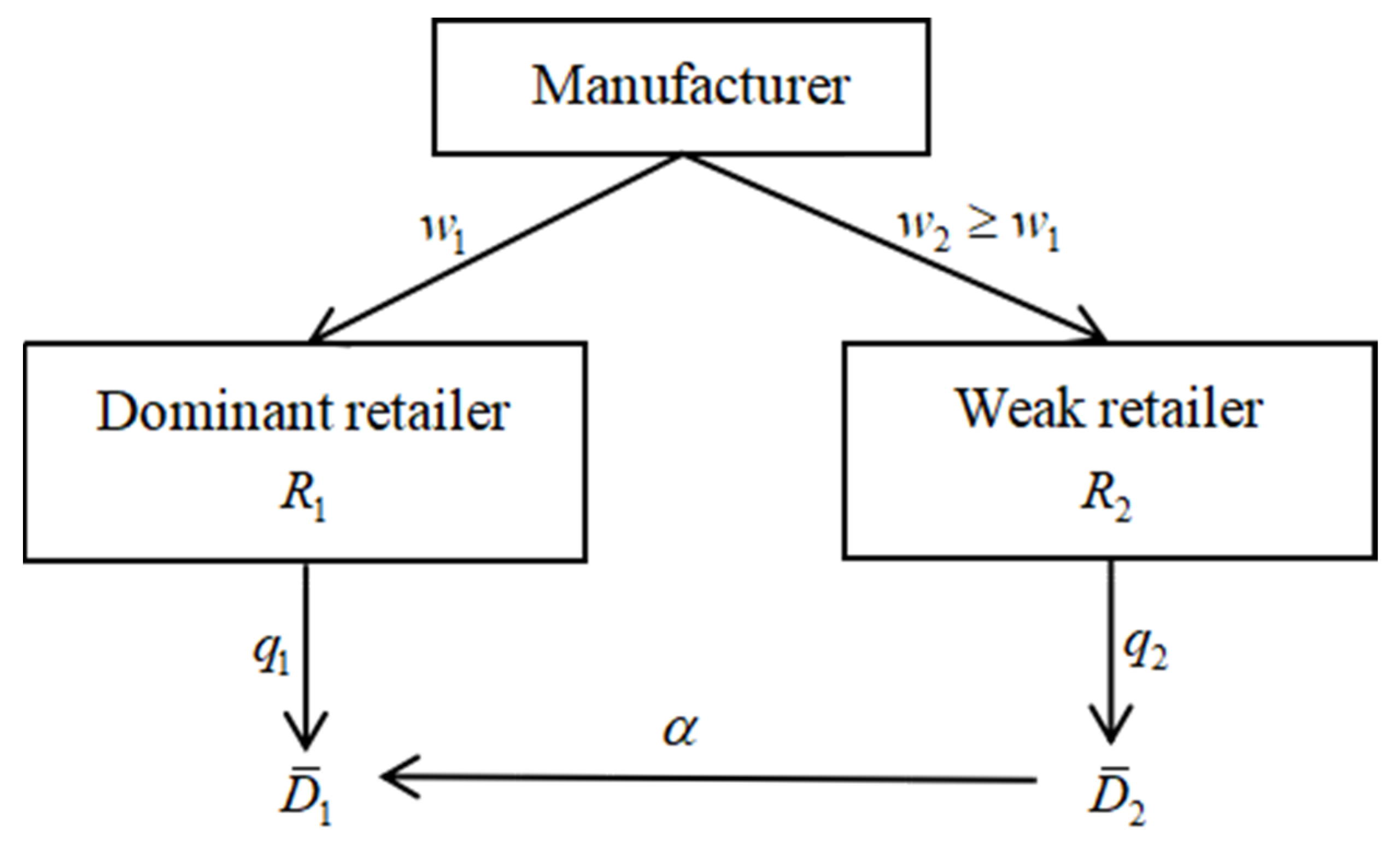
Consider a manufacturer selling a product to two differentiated retailers that compete in sales during a sales season. The retailers sell at the same exogenous retail price $p$ to the consumer. The two retailers have asymmetric bargaining power and market power. The dominant retailer ($R_1$) has a stronger bargaining power, so the manufacturer provides him with an exogenous wholesale price $w_1$. We assume that the dominant retailer’s retail price $w_1$ is endogenous and not higher than $\frac{p}{2}$. Moreover, the weak retailer ($R_2$) has less bargaining power and cannot negotiate the wholesale price with the upstream manufacturer. Therefore, the manufacturer offers a take-it or leave-it wholesale price $w_2\ge w_1$ to the weak retailer.

Market Demand. Suppose that weak retailer’s prior demand $D_2$ is the normal distributed with mean $d_2$ and variance ${\delta }^2$, i.e., $D_2~N\left(d_2,{\delta }^2\right)$, which is known to all firms. Moreover, the posterior demand $D_2^{\prime }~N\left(d_2,{\delta }^{\prime 2}\right)$ is the weak retailer’s private information. In particular, $0<{\delta }^{\prime }<\delta$ reflects the posterior information that is more valuable than the prior information. The stochastic demand $D_2$ (${D^{\prime }}_2$) has a probability density function $f_{D_2}(\cdot )$ ($f_{{D^{\prime }}_2}(\cdot )$) and a cumulative distribution function $F_{D_2}(\cdot )$ ($F_{{D^{\prime }}_2}(\cdot )$). For simplicity, we assume that $d_2$ is sufficiently large so that the probability of a negative demand can be ignored in the following.

We assume that strong retailers have a stronger ability to absorb the market demand. That is, the unmet demand of the weak retailer can be partially transferred to the dominant retailer at the demand substitution rate $\alpha \in \left(0,1\right)$, but the unmet demand of the dominant retailer cannot be transferred to the weak retailer, thus, for the weak retailer, the demand substitution rate is zero. Similar to Wu et al. (2019) [7], it is called cross-demand, and the total demand of each retailer includes the initial demand and the cross-demand. We focus on the information sharing strategy of the weak retailer in the presence of bargaining power and market power asymmetry. To make this analysis tractable, we assume that the dominant retailer’s initial demand $d_1>0$ is deterministic.

Since the weak retailer’s unmet demand can be partly transferred to the dominant retailer and its’ posterior is unknown to other players, the weak retailer may choose to share or not share with another retailer and manufacturer, or only share one of them. Therefore, if the weak retailer shares his posterior information $D_2^{\prime }$ to the dominant retailer, the total demand faced by the dominant retailer is ${\overline{D}}_1=d_1+\alpha {\left(D_2^{\prime }-q_2\right)}^{+}$, otherwise, the total demand faced by the dominant retailer is ${\overline{D}}_1=d_1+\alpha {\left(D_2-q_2\right)}^{+}$, where ${\left[a\right]}^{+}=\max \left(a,0\right)$. The total demand faced by the weak retailer is always ${\overline{D}}_2=D_2^{\prime }$.

As shown above, the weak retailer’s demand information affects the manufacturer’s wholesale price decision and the dominant retailer’s order decision. We consider the retailer’s information sharing strategy. Figure 1 illustrates the arrangement of agents.

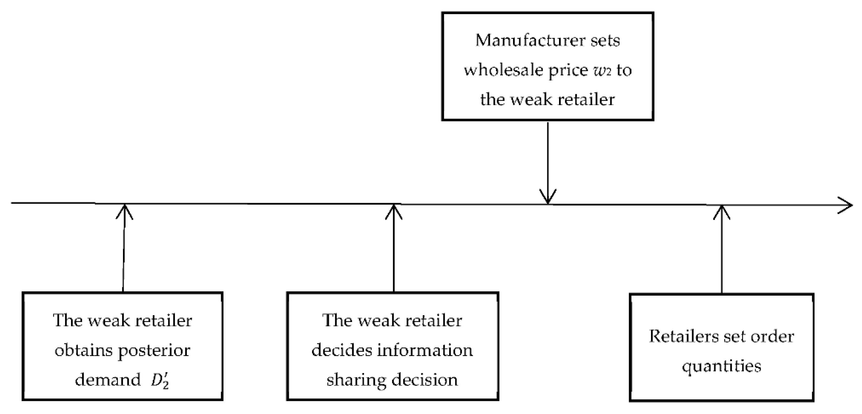
Sequence of Events. The sequence of events as follows: (1) the weaker retailer $R_2$ becomes privately informed of posterior demand $D_2^{\prime }$; (2) the weak retailer decides whether to share his private information with other players, i.e., the manufacturer and the dominant retailer; (3) the manufacturer offers an exogenous wholesale price $w_1$ to the dominant retailer and decides a take-it or leave-it wholesale price $w_2$ to the weak retailer; (4) the retailers simultaneously decide their order quantity, $q_1$ and $q_2$. The timing of the model is depicted in Figure 2.

3.1. The Weak Retailer’s Ordering Response

In the fourth stage, since the unmet demand of the dominant retailer cannot be transferred to the weak retailer, the profit of the weak retailer is only affected by its own demand ${\overline{D}}_2=D_2^{\prime }$ and wholesale price $w_2$. Therefore, the weak retailer’s expected profit is given by

$$\begin{array}{ll}{\pi }_2\left(q_2|w_2,{\overline{D}}_2\right)& =p{\rm E}\min \left(q_2,D_2^{\prime }\right)-w_2{q}_2\\ & =p{q}_2-p{\displaystyle {\int }_{-\infty }^{q_2}{F}_{D_2^{\prime }}\left(D\right)dD-}{w}_2{q}_2.\end{array}$$

(1)

Denote $\varphi (\cdot )$ as PDF of the standard normal distribution and $\mathrm{\Phi }(\cdot )$ as CDF of the standard normal distribution. Moreover, $\overline{\mathrm{\Phi }}(\cdot )=1-\mathrm{\Phi }(\cdot )$ is complementary CDF of the standard normal distribution and ${\overline{\mathrm{\Phi }}}^{-1}(\cdot )$ is inverse completed CDF of the standard normal distribution. $z(\cdot )=\frac{\varphi (\cdot )}{\overline{\mathrm{\Phi }}(\cdot )}$ is increasing failure rate (see, e.g., [45,46]). The weak retailer’s optimal order quantity in stage 4, as a function of $D_2^{\prime }$ and $w_2$, is then given by $q_2\left(w_2,D_2^{\prime }\right)={\overline{F}}_{D_2^{\prime }}{}^{-1}\left(\frac{w_2}{p}\right)=d_2+{{\delta }^{\prime }}_2{\overline{\mathrm{\Phi }}}^{-1}\left(\frac{w_2}{p}\right)$.

Note that for other players, in the case of obtaining information, the weak retailer’s response function is related to the posterior information, which is $q_2\left(w_2,D_2^{\prime }\right)$; otherwise, in the case of no information, the weak retailer’s response function is only related to the prior information, which is $q_2\left(w_2,D_2\right)=d_2+{\delta }_2{\overline{\mathrm{\Phi }}}^{-1}\left(\frac{w_2}{p}\right)$. When the wholesale price is relatively high, i.e., $w_2\in \left(\frac{p}{2},p\right]$, the information sharing increases the weak retailer’s response order quantity, i.e., $q_2\left(w_2,D_2\right)<q_2\left(w_2,D_2^{\prime }\right)<d_2$; when the wholesale price is relatively low, i.e., $w_2\in \left[0,\frac{p}{2}\right)$, the information sharing decreases the weak retailer’s response order quantity, i.e., $q_2\left(w_2,D_2\right)>q_2\left(w_2,D_2^{\prime }\right)>d_2$.

The intuition is as follows. First, if the weak retailer faces a relatively high wholesale price, he will reduce his order until it is lower than the mean of the prior demand $d_2$ whether the information is shared or not. Second, a relatively low wholesale price increases the retailer’s order until it is higher than the mean of the prior demand $d_2$ whether information is shared or not. This qualitative result reflects that the information sharing strategy does not affect the change direction of the weak retailer’s order quantity (i.e., higher than or lower than the initial demand), whereas the wholesale price $w_2$ has a very significant influence on the relationship between the weak retailer’s order quantity and the initial demand. Second, it is interesting to note that under the low (high) wholesale price, the other players will overestimate (underestimate) the weak retailer’s order quantity if the weak retailer does not share his private information.

3.2. The Dominant Retailer’s Ordering Response

In the fourth stage, if the weak retailer shares information to the dominant retailer, the dominant retailer makes the order quantity decision depending on $q_2\left(w_2,D_2^{\prime }\right)$. The dominant retailer’s expected profit is given by

$$\begin{array}{l}{\pi }_1\left(q_1|q_2\left(w_2,D_2^{\prime }\right)\right)=p{\rm E}\min \left(q_1,d_1+\alpha {\left(D_2^{\prime }-q_2\left(w_2,D_2^{\prime }\right)\right)}^{+}\right)-w_1{q}_1\\ =\{\begin{array}{l}\left(p-w_1\right)q_1, if{q}_1<d_1,\hfill \\ p\left(q_1-\alpha {\displaystyle {\int }_{q_2\left(w_2,D_2^{\prime }\right)}^{\frac{1}{\alpha }\left(q_1-d_1\right)+q_2\left(w_2,D_2^{\prime }\right)}{F}_{{D^{\prime }}_2}\left(D\right)dD}\right)-w_1{q}_1, if{q}_1\ge d_1.\hfill \end{array}\end{array}$$

(2)

The dominant retailer’s optimal order quantity in stage 4, as a function of $D_2^{\prime }$ and $w_2$, is then given by $q_1\left(w_2,D_2^{\prime }\right)=d_1+\alpha \left({\overline{F}}_{D_2^{\prime }}{}^{-1}\left(\frac{w_1}{p}\right)-q_2\left(w_2,D_2^{\prime }\right)\right)$. Thus, $q_1\left(w_2,D_2^{\prime }\right)=d_1+\alpha {\delta }^{\prime }\left({\overline{\mathrm{\Phi }}}^{-1}\left(\frac{w_1}{p}\right)-{\overline{\mathrm{\Phi }}}^{-1}\left(\frac{w_2}{p}\right)\right)$.

Similarly, if the weak retailer does not share information to the dominant retailer, the dominant retailer makes the order quantity decision depending on $q_2\left(w_2,D_2\right)$. The dominant retailer’s expected profit is given by

$$\begin{array}{l}{\pi }_1\left(q_1|q_2\left(w_2,D_2\right)\right)=p{\rm E}\min \left(q_1,d_1+\alpha {\left(D_2-q_2\left(w_2,D_2\right)\right)}^{+}\right)-w_1{q}_1\\ =\{\begin{array}{l}\left(p-w_1\right)q_1, if{q}_1<d_1,\hfill \\ p\left(q_1-\alpha {\displaystyle {\int }_{q_2\left(w_2,D_2\right)}^{\frac{1}{\alpha }\left(q_1-d_1\right)+q_2\left(w_2,D_2\right)}{F}_{D_2^{\prime }}\left(D\right)dD}\right)-w_1{q}_1, if{q}_1\ge d_1.\hfill \end{array}\end{array}$$

(3)

The dominant retailer’s optimal order quantity in stage 4, as a function of $D_1^{\prime }$, $D_2$ and $w_2$, is then given by $q_1\left(w_2,D_2\right)=d_1+\alpha \left({\overline{F}}_{D_2}{}^{-1}\left(\frac{w_1}{p}\right)-q_2\left(w_2,D_2\right)\right)$. Thus, $q_1\left(w_2,D_2\right)=d_1+\alpha \delta \left({\overline{\mathrm{\Phi }}}^{-1}\left(\frac{w_1}{p}\right)-{\overline{\mathrm{\Phi }}}^{-1}\left(\frac{w_2}{p}\right)\right)$.

It follows from the fact $w_2\ge w_1$ that the dominant retailer’s order quantity is not less than his initial demand $d_1$, regardless of whether the dominant retailer is informed or not. In particular, the dominant retailer’s order quantity is equal to his initial demand if and only if the manufacturer offers the lowest wholesale price to the weak retailer, e.g., $w_2=w_1$. When the manufacturer offers a high wholesale price $w_2$ to the weak retailer, the dominant retailer deems that the weak retailer will lower his order quantity and has a more unmet market demand, thereby increasing his order quantity, i.e., $\frac{\partial q_1\left(w_2,D_2\right)}{\partial w_2}>0$ and $\frac{\partial q_1\left(w_2,D_2^{\prime }\right)}{\partial w_2}>0$.

4. Analysis

This section presents the description and analysis of the four cases: The benchmark case with no information sharing (N), the second case in which the weak retailer only shares his posterior demand information to the dominated retailer (PR), the third case in which the weak retailer only shares his posterior demand information to the upstream manufacturer (PM), and the fourth case in which the weak retailer shares his posterior demand information to the dominated retailer and the upstream manufacturer (FS). We start with the benchmark case.

4.1. Benchmark Case: No Information Sharing (N)

In the third stage, the manufacturer decides the wholesale price $w_2$ depends on prior demand $D_2$, thus retailers’ response functions are $q_1\left(w_2,D_2\right)$ and $q_2\left(w_2,D_2\right)$, respectively. The manufacturer’s optimization problem is

$$\begin{array}{l}\underset{w_2\ge w_1}{\max }\mathrm{\Pi }\left(w_2|q_1\left(w_2,D_2\right),q_2\left(w_2,D_2\right)\right)=\underset{w_2\ge w_1}{\max }\left(w_1{q}_1\left(w_2,D_2\right)+w_2{q}_1\left(w_2,D_2\right)\right)\\ =\underset{w_2\ge w_1}{\max }\left(w_1\left(d_1+\alpha \delta \left({\overline{\mathrm{\Phi }}}^{-1}\left(\frac{w_1}{p}\right)-{\overline{\mathrm{\Phi }}}^{-1}\left(\frac{w_2}{p}\right)\right)\right)+w_2\left(d_2+\delta {\overline{\mathrm{\Phi }}}^{-1}\left(\frac{w_2}{p}\right)\right)\right)\end{array}$$

(4)

Note that the assumptions of $w_1\le \frac{p}{2}$ and $d_2$ is sufficiently large (e.g., $d_2>\frac{\delta }{z\left(0\right)}$) ensures that $p\overline{\mathrm{\Phi }}\left({\widehat{y}}_{\delta }\right)>w_1$, where ${\widehat{y}}_{\delta }<0$ solves $p\overline{\mathrm{\Phi }}\left({\widehat{y}}_{\delta }\right)\left[1-z\left({\widehat{y}}_{\delta }\right)\left({\widehat{y}}_{\delta }+\frac{d_2}{\delta }\right)\right]=\alpha w_1$. Therefore, we obtain the optimal wholesale price under no information sharing as follows.

Lemma 1.

When the weak retailer does not share demand information, the weak retailer’s wholesale price in equilibrium equals $w_2^{NS}=p\overline{\mathrm{\Phi }}\left({\widehat{y}}_{\delta }\right)$.

The intuition behind Lemma 1 is that the manufacturer’s decision of the wholesale price for the weak retailer depends not only on the prior demand information of the weak retailer, i.e., $D_2~N\left(d_2,{\delta }^2\right)$, but also on the endogenous wholesale price $w_1$ provided to another retailer.

Since the dominant retailer makes the order quantity decision based on the prior information of the weak retailer’s demand $D_2$ and wholesale prices $w_2^{NS}$, the dominant retailer’s equilibrium order quantity is $q_1^{NS}=q_1\left(w_2^{NS},D_2\right)=d_1+\alpha \delta \left({\overline{\mathrm{\Phi }}}^{-1}\left(\frac{w_1}{p}\right)-{\widehat{y}}_{\delta }\right)$. The weak retailer makes the order quantity decision based on the posterior information of his demand $D_2^{\prime }$ and wholesale prices $w_2^{NS}$, so the weak retailer’s equilibrium order quantity is $q_2^{NS}=q_2\left(w_2^{NS},D_2^{\prime }\right)=d_2+{\delta }^{\prime }{\widehat{y}}_{\delta }$.

Based on the foregoing, we derive retailers and the manufacturer’s equilibrium expected profit under no information sharing as follows.

$${\mathrm{\Pi }}^{NS}=\mathrm{\Pi }\left(w_2^{NS}|q_1^{NS},q_2^{NS}\right)=w_1\left(d_1+\alpha \delta \left({\overline{\mathrm{\Phi }}}^{-1}\left(\frac{w_1}{p}\right)-{\widehat{y}}_{\delta }\right)\right)+w_2\left(d_2+{\delta }^{\prime }{\widehat{y}}_{\delta }\right)$$

$${\pi }_1^{NS}={\pi }_1\left(q_1^{NS}|q_2^{NS}\right)=\left(p-w_1\right)\left(d_1+\alpha \delta \left({\overline{\mathrm{\Phi }}}^{-1}\left(\frac{w_1}{p}\right)-{\widehat{y}}_{\delta }\right)\right)-\alpha p{\displaystyle {\int }_{d_2+{\delta }^{\prime }{\widehat{y}}_{{\delta }_2}}^{d_2+\delta {\overline{\mathrm{\Phi }}}^{-1}\left(\frac{w_1}{p}\right)-\left(\delta -{\delta }^{\prime }\right){\widehat{y}}_{\delta }}{F}_{D_2^{\prime }}\left(D\right)dD;\mathrm{and}}$$

$${\pi }_2^{NS}={\pi }_2\left(q_2^{NS}|w_1^{NS},D_2^{\prime }\right)=p\mathrm{\Phi }\left({\widehat{y}}_{\delta }\right)\left(d_2+{\delta }^{\prime }{\widehat{y}}_{\delta }\right)-p{\displaystyle {\int }_{-\infty }^{d_2+{\delta }^{\prime }{\widehat{y}}_{\delta }}{F}_{D_2^{\prime }}\left(D\right)dD}$$

4.2. With the Dominant Retailer (PR)

In the third stage, the manufacturer makes the wholesale price decision depending on prior demand $D_2$, thus the manufacturer’s expected profit is the same as that without information sharing. Furthermore, we get that the equilibrium wholesale price is $w_2^{PR}=p\overline{\mathrm{\Phi }}\left({\widehat{y}}_{\delta }\right)$. The dominant retailer’s equilibrium order quantity is $q_1^{PR}=q_1\left(w_2^{NS},D_2^{\prime }\right)=d_1+\alpha {\delta }^{\prime }\left({\overline{\mathrm{\Phi }}}^{-1}\left(\frac{w_1}{p}\right)-{\widehat{y}}_{\delta }\right)$, and the weak retailer’s equilibrium order quantity is $q_2^{PR}=q_2\left(w_2^{PR},D_2^{\prime }\right)=d_2+{\delta }^{\prime }{\widehat{y}}_{{\delta }^{\prime }}$. Since the dominant retailer knows the posterior demand, the dominant retailer’s equilibrium order quantity is related to $D_2^{\prime }$.

When the weak retailer only shares information with the dominant retailer, the retailers and the manufacturers’ equilibrium expected profit as follows.

$${\mathrm{\Pi }}^{PR}=\mathrm{\Pi }\left(w_2^{PR}|q_1^{PR},q_2^{PR}\right)=w_1\left(d_1+\alpha {\delta }^{\prime }\left({\overline{\mathrm{\Phi }}}^{-1}\left(\frac{w_1}{p}\right)-{\widehat{y}}_{\delta }\right)\right)+p\overline{\mathrm{\Phi }}\left({\widehat{y}}_{\delta }\right)\left(d_2+{\delta }^{\prime }{\widehat{y}}_{\delta }\right)$$

$${\pi }_1^{PR}={\pi }_1\left(q_1^{PR}|q_2^{PR}\right)=\left(p-w_1\right)\left(d_1+\alpha {\delta }^{\prime }\left({\overline{\mathrm{\Phi }}}^{-1}\left(\frac{w_1}{p}\right)-{\widehat{y}}_{\delta }\right)\right)-\alpha p{\displaystyle {\int }_{d_2+{\delta }^{\prime }{\widehat{y}}_{\delta }}^{d_2+{\delta }^{\prime }{\overline{\mathrm{\Phi }}}^{-1}\left(\frac{w_1}{p}\right)}{F}_{D_2^{\prime }}\left(D\right)dD;\mathrm{and}}$$

$${\pi }_2^{PR}={\pi }_2\left(q_2^{PR}|w_2^{PR},D_2^{\prime }\right)=p\mathrm{\Phi }\left({\widehat{y}}_{\delta }\right)\left(d_2+{\delta }^{\prime }{\widehat{y}}_{\delta }\right)-p{\displaystyle {\int }_{-\infty }^{d_2+{\delta }^{\prime }{\widehat{y}}_{\delta }}{F}_{D_2^{\prime }}\left(D\right)dD}$$

4.3. With the Manufacturer (PM)

In the third stage, if the weak retailer only shares information with the manufacturer, for the manufacturer, the retailers’ response functions are $q_1\left(w_2,D_2\right)$ and $q_2\left(w_2,D_2^{\prime }\right)$, respectively. The manufacturer’s optimization problem is

$$\begin{array}{l}\underset{w_2\ge w_1}{\max }\mathrm{\Pi }\left(w_2|q_1\left(w_2,D_2\right),q_2\left(w_2,D_2^{\prime }\right)\right)=\underset{w_2\ge w_1}{\max }\left(w_1{q}_1\left(w_2,D_2\right)+w_2{q}_1\left(w_2,D_2^{\prime }\right)\right)\\ =\underset{w_2\ge w_1}{\max }\left(w_1\left(d_1+\alpha \delta \left({\overline{\mathrm{\Phi }}}^{-1}\left(\frac{w_1}{p}\right)-{\overline{\mathrm{\Phi }}}^{-1}\left(\frac{w_2}{p}\right)\right)\right)+w_2\left(d_2+{\delta }^{\prime }{\overline{\mathrm{\Phi }}}^{-1}\left(\frac{w_2}{p}\right)\right)\right).\end{array}$$

(5)

Lemma 2.

When the weak retailer only shares information with the manufacturer, the weak retailer’s wholesale price in equilibrium equals$w_2^{PM}=p\overline{\mathrm{\Phi }}\left({\widehat{y}}_{\delta ,{\delta }^{\prime }}\right)$, where${\widehat{y}}_{\delta ,{\delta }^{\prime }}<0$solves$p{\delta }^{\prime }\overline{\mathrm{\Phi }}\left({\widehat{y}}_{\delta ,{\delta }^{\prime }}\right)\left[1-z\left({\widehat{y}}_{\delta ,{\delta }^{\prime }}\right)\left({\widehat{y}}_{\delta ,{\delta }^{\prime }}+\frac{d_2}{{\delta }^{\prime }}\right)\right]=\alpha \delta w_1$.

The intuition behind Lemma 2 is that when the weak retailer only shares information with the manufacturer, the manufacturer makes the wholesale price dependent on both a priori and a posterior demand information of the weak retailer, i.e., $D_2\sim N\left(d_2,{\delta }^2\right)$ and $D_2^{\prime }\sim N\left(d_2,{{\delta }^{\prime }}^2\right)$. This is because the manufacturer obtains the posterior demand information directly from the weak retailer and makes the decision according to the dominant retailer’s response of the order quantity related to the prior information.

Since the dominant retailer makes the order quantity decision based on the prior information of the weak retailer’s initial demand $D_2$ and wholesale prices $w_2^{PM}$, the dominant retailer’s equilibrium order quantity is $q_1^{PM}=q_1\left(w_2^{PM},D_2\right)=d_1+\alpha \delta \left({\overline{\mathrm{\Phi }}}^{-1}\left(\frac{w_1}{p}\right)-{\widehat{y}}_{\delta ,{\delta }^{\prime }}\right)$. The weak retailer makes its ordering quantity based on the posterior information of his initial demand $D_2^{\prime }$ and wholesale prices $w_2^{PM}$, so the weak retailer’s equilibrium order quantity is $q_2^{PM}=q_2\left(w_2^{PM},D_2^{\prime }\right)=d_2+{\delta }^{\prime }{\widehat{y}}_{\delta ,{\delta }^{\prime }}$.

Furthermore, when the weak retailer only shares information with the manufacturer, the retailers’ and the manufacturer’s equilibrium expected profit are as follows.

$${\mathrm{\Pi }}^{PM}=\mathrm{\Pi }\left(w_2^{PM}|q_1^{PM},q_2^{PM}\right)=w_1\left(d_1+\alpha \delta \left({\overline{\mathrm{\Phi }}}^{-1}\left(\frac{w_1}{p}\right)-{\widehat{y}}_{\delta ,{\delta }^{\prime }}\right)\right)+p\overline{\mathrm{\Phi }}\left({\widehat{y}}_{\delta ,{\delta }^{\prime }}\right)\left(d_2+{\delta }^{\prime }{\widehat{y}}_{\delta ,{\delta }^{\prime }}\right)$$

$$\begin{array}{l}{\pi }_1^{PM}={\pi }_1\left(q_1^{PM}|q_2^{PM}\right)\\ =\left(p-w_1\right)\left(d_1+\alpha \delta \left({\overline{\mathrm{\Phi }}}^{-1}\left(\frac{w_1}{p}\right)-{\widehat{y}}_{{\delta }_2,{\delta }_2^{\prime }}\right)\right)-\alpha p{\displaystyle {\int }_{d_2+{\delta }^{\prime }{\widehat{y}}_{{\delta }_2,{{\delta }^{\prime }}_2}}^{d_2+{\delta }^{\prime }{\overline{\mathrm{\Phi }}}^{-1}\left(\frac{w_1}{p}\right)-\left({\delta }_2-{\delta }_2^{\prime }\right){\widehat{y}}_{{\delta }_2,{\delta }_2^{\prime }}}{F}_{D_2^{\prime }}\left(D\right)dD}\end{array};\mathrm{and}$$

$${\pi }_2^{PM}={\pi }_2\left(q_2^{PM}|w_2^{PM},D_2^{\prime }\right)=p\mathrm{\Phi }\left({\widehat{y}}_{\delta ,{\delta }^{\prime }}\right)\left(d_2+{\delta }^{\prime }{\widehat{y}}_{\delta ,{\delta }^{\prime }}\right)-p{\displaystyle {\int }_{-\infty }^{d_2+{\delta }^{\prime }{\widehat{y}}_{\delta ,{\delta }^{\prime }}}{F}_{D_2^{\prime }}\left(D\right)dD.}$$

4.4. With the Dominant Retailer and the Manufacturer (FS)

In the third stage, if the weak retailer shares information with the manufacturer and the dominant retailer, the retailers’ response functions are $q_1\left(w_2,D_2^{\prime }\right)$ and $q_2\left(w_2,D_2^{\prime }\right)$, respectively. The manufacturer’s optimization problem is

$$\begin{array}{l}\underset{w_2\ge w_1}{\max }\mathrm{\Pi }\left(w_2|q_1\left(w_2,D_2^{\prime }\right),q_2\left(w_2,D_2^{\prime }\right)\right)=\underset{w_2\ge w_1}{\max }\left(w_1{q}_1\left(w_2,D_2^{\prime }\right)+w_2{q}_1\left(w_2,D_2^{\prime }\right)\right)\\ =\underset{w_2\ge w_1}{\max }\left(w_1\left(d_1+\alpha {\delta }^{\prime }\left({\overline{\mathrm{\Phi }}}^{-1}\left(\frac{w_1}{p}\right)-{\overline{\mathrm{\Phi }}}^{-1}\left(\frac{w_2}{p}\right)\right)\right)+w_2\left(d_2+{\delta }^{\prime }{\overline{\mathrm{\Phi }}}^{-1}\left(\frac{w_2}{p}\right)\right)\right).\end{array}$$

(6)

Lemma 3.

When the weak retailer shares information with both, the weak retailer’s wholesale price in equilibrium equals$w_2^{FS}=p\overline{\mathrm{\Phi }}\left({\widehat{y}}_{{\delta }^{\prime }}\right)$, where${\widehat{y}}_{{\delta }^{\prime }}<0$solves$p\overline{\mathrm{\Phi }}\left({\widehat{y}}_{{\delta }^{\prime }}\right)\left[1-z\left({\widehat{y}}_{{\delta }^{\prime }}\right)\left({\widehat{y}}_{{\delta }^{\prime }}+\frac{d_2}{{\delta }^{\prime }}\right)\right]=\alpha w_1$.

Lemma 3 shows that when the weak retailer shares information with both, the manufacturer makes the wholesale price depend on the posterior demand information of the weak retailer, i.e., $D_2^{\prime }\sim N\left(d_2,{{\delta }^{\prime }}^2\right)$.

Since retailers make order quantities based on the posterior information of the initial demand $D_2^{\prime }$, the dominant retailer’s equilibrium order quantity is $q_1^{FS}=q_1\left(w_2^{FS},D_2^{\prime }\right)=d_1+\alpha {\delta }^{\prime }\left({\overline{\mathrm{\Phi }}}^{-1}\left(\frac{w_1}{p}\right)-{\widehat{y}}_{{\delta }^{\prime }}\right)$ and the weak retailer’s equilibrium order quantity is $q_2^{FS}=q_2\left(w_2^{FS},D_2^{\prime }\right)=d_2+{\delta }^{\prime }{\widehat{y}}_{{\delta }^{\prime }}$.

Furthermore, when the weak retailer shares information with both, the retailers’ and the manufacturer’s equilibrium expected profit are as follows.

$${\mathrm{\Pi }}^{FS}=\mathrm{\Pi }\left(w_2^{FS}|q_1^{FS},q_2^{FS}\right)=w_1\left(d_1+\alpha {\delta }^{\prime }\left({\overline{\mathrm{\Phi }}}^{-1}\left(\frac{w_1}{p}\right)-{\widehat{y}}_{{\delta }^{\prime }}\right)\right)+p\overline{\mathrm{\Phi }}\left({\widehat{y}}_{{\delta }^{\prime }}\right)\left(d_2+{\delta }^{\prime }{\widehat{y}}_{{\delta }^{\prime }}\right)$$

$$\begin{array}{l}{\pi }_1^{FS}={\pi }_1\left(q_1^{FS}|q_2^{FS}\right)\\ =\left(p-w_1\right)\left(d_1+\alpha {\delta }^{\prime }\left({\overline{\mathrm{\Phi }}}^{-1}\left(\frac{w_1}{p}\right)-{\widehat{y}}_{{\delta }^{\prime }}\right)\right)-\alpha p{\displaystyle {\int }_{d_2+{\delta }^{\prime }{\widehat{y}}_{{\delta }^{\prime }}}^{d_2+{\delta }^{\prime }{\overline{\mathrm{\Phi }}}^{-1}\left(\frac{w_1}{p}\right)}{F}_{D_1^{\prime }}\left(D\right)dD}\end{array};\mathrm{and}$$

$${\pi }_2^{FS}={\pi }_2\left(q_2^{FS}|w_2^{FS},D_2^{\prime }\right)=p\mathrm{\Phi }\left({\widehat{y}}_{{\delta }^{\prime }}\right)\left(d_2+\alpha {\delta }^{\prime }{\widehat{y}}_{{\delta }^{\prime }}\right)-p{\displaystyle {\int }_{-\infty }^{d_2+{\delta }^{\prime }{\widehat{y}}_{{\delta }^{\prime }}}{F}_{D_2^{\prime }}\left(D\right)dD.}$$

5. Format Preferences

We first compare the impact of the four information sharing formats on the retailers’ ordering decisions and the manufacturer’s wholesale price decision, and then examine the firms’ preference over the four information sharing formats.

5.1. The Effect of Information Sharing on the Firms’ Decisions

Proposition 1.

The manufacturer sets the highest wholesale price to the weak retailer when the weak retailer’s partial shares demand information with the manufacturer. Moreover, the manufacturer sets the lowest wholesale price to the weak retailer when the weak retailer doesn’t share the demand information with both players or only partially shares the demand information with the dominant retailer, i.e., $w_2^{NS}=w_2^{PR}<w_2^{FS}<w_2^{PM}$.

Proposition 1 shows that among the four information-sharing formats, the “partial sharing with the manufacturer” format makes the manufacturer charge the highest wholesale price. However, the “partial sharing with the dominant retailer” format and the “no information sharing” format make the manufacturer charge the lowest wholesale price.

The intuition behind Proposition 1 is that the manufacturer’s understanding of the demand information of the weak retailer determines the level of the wholesale price provided to the weak retailer. Specifically, compared with the other three information sharing formats, in the format of when the weak retailer only shares demand information with the manufacturer, the manufacturer can use the information advantage to set a higher wholesale price, thereby obtaining more sales revenue. Under the two formats of when the weak retailer doesn’t share demand information with both players or only partially shares demand information with the dominant retailer, the manufacturer is at a disadvantage of information, so it can only set the lowest wholesale price. Apart from the above, when the weak retailer shares demand information to all participants, the manufacturer has the same information advantage as other participants, so he will set an intermediate wholesale price.

Proposition 2.

The weak retailer orders the most products when the weak retailer does not share information with any players or only partially shares demand information with the dominant retailer. Moreover, the weak retailer orders the least amount of products when the weak retailer only partially shares their demand information with the manufacturer, i.e., $q_2^{PM}<q_2^{FS}<q_2^{NS}=q_2^{PR}$.

Proposition 2 shows that among the four information-sharing formats, the “partial sharing with the dominant retailer” format and the “no information sharing” format promote the weak retailer to order products without difference. However, the “partial sharing with the manufacturer” format restricts the weak retailer from ordering products. This is because the weak retailer’s information sharing strategy affects the upstream manufacturer’s wholesale price decision, which in turn affects the weak retailer’s ordering decision. Thus, in equilibrium, the weak retailer’s order quantity responds negatively to the wholesale price provided by the manufacturer.

Proposition 3.

The dominant retailer orders the most (least) products when the weak retailer only partially shares the demand information with the manufacturer (the dominant retailer), i.e., $q_1^{PM}=\underset{k=NS,PR,PM,FS}{\max }{q}_1^k$and$q_1^{PR}=\underset{k=NS,PR,PM,FS}{\min }{q}_1^k$.

Proposition 3 shows that among the four information-sharing formats, the “partial sharing with the manufacturer” format promotes the dominant retailer to order products. However, the “partial sharing with the dominant retailer” format restricts the dominant retailer from ordering products.

Recall that the manufacturer provides the dominant retailer with an exogenous wholesale price but provides the weak retailer with an endogenous wholesale price, and the unmet demand of the weak retailer can transfer to the dominant retailer. Therefore, the dominant retailer’s order quantity is affected by the wholesale price accepted by the weak retailer, and the information strategy and the order quantity of the weak retailer. Specifically, when only the manufacturer is informed of the weak retailer’s demand information, the dominant retailer orders the most products, i.e., $q_1^{PM}=\underset{k=NS,PR,PM,FS}{\max }{q}_1^k$. This is because that under this format, the manufacturer charges the highest wholesale price to the weak retailer, i.e., $w_2^{PM}>\underset{k=PR,NS,FS}{\max }{w}_2^k$, thereby lowering the weak retailer’s order quantity, i.e., $q_2^{PM}<\underset{k=PR,NS,FS}{\min }{q}_2^k$, and transferring more unmet demand to the dominant retailer. When only the dominant retailer is informed of the weak retailer’s demand information, the dominant retailer orders the least amount of products, i.e., $q_1^{PR}=\underset{k=NS,PR,PM,FS}{\min }{q}_1^k$. This is because, under this format, the manufacturer charges the least wholesale price to the weak retailer, i.e., $w_2^{PR}=\underset{k=PR,PM,NS,FS}{\min }{w}_2^k$, thereby increasing the weak retailer’s order quantity, i.e., $q_2^{PR}=\underset{k=PR,PM,NS,FS}{\max }{q}_2^k$, and transferring less unmet demand to the dominant retailer. From Proposition 1 and Proposition 2, the manufacturer (the weak retailer) makes the same wholesale price decision (order quantity decision) under the “no information sharing” format and the “partial sharing with the dominant retailer” format, i.e., $w_2^{NS}=w_2^{PR}$ and $q_2^{NS}=q_2^{PR}$. However, the dominant retailer’s order is less when only the dominant retailer is informed of the weak retailer decision, i.e., $q_1^{PR}<q_1^{NS}$. This is because, under the “no information sharing” format, the dominant retailer’s prediction accuracy of the initial demand of the weak retailer is lower, i.e., $\delta >{\delta }^{\prime }$, which improves the dominant retailer’s order quantity to meet the relatively more uncertain market demand compared with the “partial sharing with the dominant retailer” format.

5.2. The Effect of Information Sharing on Firms’ Profits

Proposition 4.

In equilibrium, the weak retailer gains the highest equilibrium expected profit under the “no information sharing” format and the “partial sharing with the dominant retailer” format, and the lowest equilibrium expected profit under the “partial sharing with the manufacturer” format, i.e.,${\pi }_2^{PM}<{\pi }_2^{FS}<{\pi }_2^{NS}={\pi }_2^{PR}$.

Proposition 4 shows that the weak retailer prefers the “no information sharing” format and the “partial sharing with the dominant retailer” format. Moreover, the retailer is least willing to partially share information with the upstream manufacturer. As Section 4 shows, the weak retailer knows the total demand he faces, and his equilibrium expected profit depends on the wholesale price, determined by the manufacturer and his order quantity. When faced with a lower wholesale price, the weak retailer will increase his order quantity, and enjoy a lower marginal ordering cost, obtain more sales revenue, and ultimately obtain the higher equilibrium expected profit. On the contrary, when faced with a higher wholesale price, the weak retailer will decrease his order quantity, to enjoy a higher marginal ordering cost and obtain less sales revenue, and ultimately obtain the lower equilibrium expected profit. The implication of Proposition 4 is that the retailer is worse off by sharing his private demand information to the upstream manufacturer (discussed in [33]). This is because of the direct effect, i.e., the manufacturer’s use of better information to seek more economic benefits and damage the interests of the retailer.

Proposition 5.

In equilibrium, the manufacturer gains the highest equilibrium expected profit under the “partial sharing with the manufacturer” format and the lowest equilibrium expected profit under the “partial sharing with the dominant retailer” format, i.e., ${\mathrm{\Pi }}^{PM}>\underset{k=PR,NS,FS}{\max }{\mathrm{\Pi }}_1^k$and${\mathrm{\Pi }}^{PR}<\underset{k=PM,NS,FS}{\max }{\mathrm{\Pi }}_1^k$.

Proposition 5 shows that the manufacturer prefers the “partial sharing with the manufacturer” format, i.e., ${\mathrm{\Pi }}^{PM}>\underset{k=PR,NS,FS}{\max }{\mathrm{\Pi }}^k$, because that the PM format enables the manufacturer to earn more profit from the dominant retailer and more marginal gains from the weak retailer. Specifically, under the PM format, the manufacturer sets the highest wholesale price to the weak retailer, i.e., $w_2^{PM}>\underset{k=PR,NS,FS}{\max }{w}_2^k$, it reduces the weak retailer’s order quantity and increases unmet market demand, i.e., $q_2^{PM}<\underset{k=PR,NS,FS}{\min }{q}_2^k$, which in turn increases the dominant retailer’s order quantity, i.e.,$q_1^{PM}>\underset{k=PR,NS,FS}{\max }{q}_1^k$. Moreover, the manufacturer is least willing to partially share information with the dominant retailer (PR), i.e., ${\mathrm{\Pi }}^{PR}<\underset{k=PM,NS,FS}{\min }{\mathrm{\Pi }}^k$, because that the PR format enables the manufacturer to earn less from profit from the dominant retailer and less marginal gains from the weak retailer. Specifically, under the PR format, the manufacturer sets the lowest wholesale price to the weak retailer, i.e., $w_2^{PR}\le \underset{k=PM,NS,FS}{\max }{w}_2^k$, it increases the weak retailer’s order quantity and decreases the unmet market demand, i.e., $q_2^{PR}\ge \underset{k=PM,NS,FS}{\max }{q}_2^k$, which in turn decreases the dominant retailer’s order quantity, i.e., $q_1^{PR}<\underset{k=PM,NS,FS}{\max }{q}_1^k$. The implication of Proposition 5 is that the manufacturer is better off by receiving the downstream retailer’s private information (discussed in [33]).

Proposition 6.

In equilibrium, the dominant retailer gains a more equilibrium expected profit under the “full information sharing” format than that under the “partial sharing with the dominant retailer” format. Moreover, the dominant retailer gains a more equilibrium expected profit under the “partial sharing with the dominant retailer” format than that under the “no information sharing” format, i.e., ${\pi }_1^{FS}>{\pi }_1^{PR}>{\pi }_1^{NS}$.

Proposition 6 shows that the dominant retailer prefers the “full information sharing” format than the “partial sharing with the dominant retailer” format. This is because compared with the PR format, the FS format increases the manufacturer’s wholesale price to the weaker retailer, i.e., $w_2^{PR}<w_2^{FS}$, thus reducing the order quantity of the weaker retailer, i.e., $q_2^{FS}<q_2^{PR}$, and increasing the unmet demand transferred from the weaker retailer. Moreover, the dominant retailer prefers the “partial sharing with the dominant retailer” format than the “no information sharing” format. Recall that the manufacturer (the weak retailer) makes the same wholesale price decision (order quantity decision) under the “no information sharing” format and the “partial sharing with the dominant retailer” format, i.e., $w_2^{NS}=w_2^{PR}$ and $q_2^{NS}=q_2^{PR}$. This shows that the understanding of information is the reason why the dominant retailer gets a higher profit under the PR format. Specifically, compared with the NS format, the dominant retailer has a more accurate understanding of the demand information of the weak retailer under the PR format, thereby reducing the loss caused by over ordering, i.e., $q_1^{PR}<q_1^{NS}$.

The implication of Proposition 6 is that when the dominant retailer is informed of the demand information of the weak retailer, the dominant retailer also wants the manufacturer to be informed of the demand information of the weak retailer. When the manufacturer is uninformed of the demand information of the weak retailer, the dominant retailer wants to be informed of the demand information of the weak retailer. Moreover, the dominant retailer’s profit does not simply depend on his order quantity or the total demand faced by him, but on the consistency between his order quantity and total demand faced by him.

5.3. The Effect of the Demand Substitution Rate

From Section 4, we learn that the demand substitution rate $\alpha$ affects the aggregate demand of the dominant retailer, which in turn changes the manufacturer’s wholesale price decision for the weaker retailer, and ultimately affects the weaker retailer’s ordering decision. Therefore, the demand substitution rate can change the decisions and benefits across all firms in the supply chain. We have the following results.

Corollary 1.

$\frac{\partial q_1^k}{\partial \alpha }>0$, $\frac{\partial q_2^K}{\partial \alpha }<0$, $\frac{\partial w_2^k}{\partial \alpha }>0$, where$k=FS,NS,PM,PR$.

Corollary 1 shows that, regardless of the information sharing format, the dominant retailer’s order quantity increases as the demand substitution rate increase, the weak retailer’s order quantity decreases as the demand substitution rate increases, and the wholesale price increases as the demand substitution rate increases. This is because the higher demand substitution rate leads to the transfer of a more unmet demand from the weak retailer to the dominant retailer, which increases the total demand faced by the dominant retailer. Therefore, the dominant retailer will increase his order quantity to meet the higher market demand. Knowing that the higher order quantity can be obtained from the dominant retailer, the manufacturer tends to the obtain the higher profits by increasing the wholesale price provided to the weak retailer, thus the weak retailer orders less quantity.

The intuition behind Corollary 1 is that in a supply chain of a manufacturer selling to two asymmetric retailers engaged in inventory competition, the demand substitution rate has an opposite effect on the inventory competitiveness of the two retailers.

Corollary 2.

$\frac{\partial {\mathrm{\Pi }}^k}{\partial \alpha }>0$, where$k=FS,NS,PM,PR$.

Corollary 2 shows that, regardless of the information sharing format, the manufacturer’s equilibrium expected profit increases as the demand substitution rate increases. This is because a higher demand substitution rate increases the dominant retailer’s effective market demand, thus inducing that the manufacturer receives more orders from the dominant retailer and sets a higher wholesale price to the weak retailer.

The implication behind the Corollary 2 is that the manufacturer prefers a higher demand substitution rate to increase the dominant retailer’s order quantity and increase marginal income from the weak retailer, thus increasing his sales revenue.

Corollary 3.

$\frac{\partial {\pi }_2^K}{\partial \alpha }<0$, where$k=FS,NS,PM,PR$.

Corollary 3 shows that, regardless of the information sharing format, the weak retailer’s equilibrium expected profit decreases as the demand substitution rate increases. This is because a higher demand substitution rate increases the weak retailer’s order cost and reduces his order quantity, thus decreasing the weak retailer’s profit.

6. Conclusions

6.1. Main Findings

In this paper, we examine four information-sharing formats (no information sharing, only sharing with the dominant retailer, only sharing with the manufacturer, and full information sharing) in a supply chain where the manufacturers selling to two asymmetric retailers engaged in inventory competition. The two competing retailers are asymmetric in a marker power over demand and bargaining power over the wholesale price. We determine the explicit solutions of the retailer’s equilibrium order quantity and the manufacturer’s equilibrium wholesale price under four information-sharing formats.

We find that there is no difference in the retailers’ preference for no information sharing and partial information sharing, since these two formats lower the wholesale price and increase the weak retailer’s order quantity. Meanwhile, we show that the dominant retailer prefers the “full information sharing” format than the “partial sharing with the dominant retailer” format since the former format increases the manufacturer’s wholesale price to the weaker retailer, thus reducing the order quantity of the weaker retailer and increasing the unmet demand transferred from the weaker retailer. Moreover, the dominant retailer prefers the “partial sharing with the dominant retailer” format than the “no information sharing” format since the dominant retailer has a more accurate understanding of the demand information of the weak retailer under the former format, thereby reducing the loss caused by over ordering. The manufacturer prefers only sharing with the manufacturer format, the main reason is that this increases the manufacturer’s wholesale price to the weak retailer.

6.2. Implications Related to Sustainability

From the findings of this study, some implications for supply chain sustainability can be concluded as follows.

First, with the development of advanced information technology, it is possible to exchange information among members of the supply chain. In addition, information technology is also a key driver of an efficient supply chain and contributes to the supply chain sustainability. Specifically, digital twin, AI, 5G and other advanced technologies have been well applied in the supply chain and promoted information sharing among supply chain members. Therefore, when supply chain members decide on information sharing strategy, it is necessary to consider the application of advanced technology to ensure the efficient and secure transmission of information.

Second, this work also serves as a theoretical basis for the application of advanced information technology in the supply chain. The application of information systems requires specific supply chain scenarios, which involve the number of supply chain members and their relationships. In fact, supply chain managers should not only introduce advanced information systems, but also consider the relations between supply chain members to ensure the supply chain sustainability. This paper considers a common situation in reality, that is, information sharing in a two-level supply chain with one manufacturer and two asymmetric competing retailers, which provides a specific scenarios for the application of information technology in the supply chain.

6.3. Future Directions

This work reveals some interesting directions for future work. First, we assume that the unilateral demand switching for future research should investigate the impact of bilateral demand switching as well. Second, this work considers a single-period model. It will be interesting to investigate how ordering and pricing decisions change in a multi-period model. Third, we assume the retailers have more market demand information and focus their information sharing strategy of the downstream retailers. Nevertheless, in some industries (e.g., fashion and apparel), large manufacturers have more market information. It is worth considering the case when the upstream manufacturer has an information advantage. Finally, in terms of the supply chain sustainability, although we have put forward some management insights, we lack to consider the measurement of the supply chain sustainability. In future research, we can consider the impact of different information sharing formats on the supply chain sustainability from the perspective of measurement.

References

- Kumar, N. The power of trust in manufacturer-retailer relationships. Harv. Bus. Rev. 1996, 74, 92. [Google Scholar]
- Dukes, A.J.; Gal-Or, E.; Srinivasan, K. Channel bargaining with retailer asymmetry. J. Mark. Res. 2006, 43, 84–97. [Google Scholar] [CrossRef]
- Geylani, T.; Dukes, A.J.; Srinivasan, K. Strategic manufacturer response to a dominant retailer. Mark. Sci. 2007, 26, 164–178. [Google Scholar] [CrossRef]
- Hua, Z.; Li, S. Impacts of demand uncertainty on retailer’s dominance and manufacturer-retailer supply chain cooperation. Omega 2008, 36, 697–714. [Google Scholar] [CrossRef]
- Bresnahan, T.F. Empirical studies of industries with market power. Handb. Ind. Organ. 1989, 2, 1011–1057. [Google Scholar]
- Amrouche, N.; Yan, R. Can a weak retailer benefit from manufacturer-dominant retailer alliance? J. Retail. Consum. Serv. 2013, 20, 34–42. [Google Scholar] [CrossRef]
- Wu, D.; Zhang, B.; Baron, O. A trade credit model with asymmetric competing retailers. Prod. Oper. Manag. 2019, 28, 206–231. [Google Scholar] [CrossRef] [Green Version]
- Bloom, P.N.; Perry, V.G. Retailer power and supplier welfare: The case of Wal-Mart. J. Retail. 2001, 77, 379–396. [Google Scholar] [CrossRef]
- Mottner, S.; Smith, S. Wal-Mart: Supplier performance and market power. J. Bus. Res. 2009, 62, 535–541. [Google Scholar] [CrossRef]
- Morris, T. Tesco: A Case Study in Supermarket Excellence. Coriolis Res. 2004. Available online: https://www.coriolisresearch.com/reports/coriolis-tesco-study-in-excellence (accessed on 4 September 2022).
- Palmer, M. Retail multinational learning: A case study of Tesco. Int. J. Retail Distrib. Manag. 2005, 33, 23–48. [Google Scholar] [CrossRef]
- Aiello, L.M.; Quercia, D.; Schifanella, R.; Del Prete, L. Tesco Grocery 1.0, a large-scale dataset of grocery purchases in London. Sci. Data 2020, 7, 57. [Google Scholar] [CrossRef] [Green Version]
- Knight, D. Surplus of home improvement stores make Indianapolis handyman heaven. In Knight Ridder Tribune Business News; Tribune Company: Chicago, IL, USA, 2003. [Google Scholar]
- Porter, M.E. Consumer behavior, retailer power and market performance in consumer goods industries. Rev. Econ. Stat. 1974, 56, 419–436. [Google Scholar] [CrossRef]
- Iyer, G.; Villas-Boas, J.M. A bargaining theory of distribution channels. J. Mark. Res. 2003, 40, 80–100. [Google Scholar] [CrossRef] [Green Version]
- Khatib, E.J.; Barco, R. Optimization of 5G networks for smart logistics. Energies 2021, 14, 1758. [Google Scholar] [CrossRef]
- Hussain, M.; Javed, W.; Hakeem, O.; Yousafzai, A.; Younas, A.; Awan, M.J.; Nobanee, H.; Zain, A.M. Blockchain-Based IoT Devices in Supply Chain Management: A Systematic Literature Review. Sustainability 2021, 13, 13646. [Google Scholar] [CrossRef]
- Kegenbekov, Z.; Jackson, I. Adaptive Supply Chain: Demand–Supply Synchronization Using Deep Reinforcement Learning. Algorithms 2021, 14, 240. [Google Scholar] [CrossRef]
- Abideen, A.Z.; Sundram, V.P.K.; Pyeman, J.; Othman, A.K.; Sorooshian, S. Digital twin integrated reinforced learning in supply chain and logistics. Logistics 2021, 5, 84. [Google Scholar] [CrossRef]
- Lee, H.L.; So, K.C.; Tang, C.S. The value of information sharing in a two-level supply chain. Manag. Sci. 2000, 46, 626–643. [Google Scholar] [CrossRef] [Green Version]
- Cachon, G.P.; Lariviere, M.A. Contracting to assure supply: How to share demand forecasts in a supply chain. Manag. Sci. 2001, 47, 629–646. [Google Scholar] [CrossRef] [Green Version]
- Terwiesch, C.; Ren, Z.J.; Ho, T.H.; Cohen, M.A. An empirical analysis of forecast sharing in the semiconductor equipment supply chain. Manag. Sci. 2005, 51, 208–220. [Google Scholar] [CrossRef] [Green Version]
- Jiang, B.; Tian, L.; Xu, Y.; Zhang, F. To share or not to share: Demand forecast sharing in a distribution channel. Mark. Sci. 2016, 35, 800–809. [Google Scholar] [CrossRef] [Green Version]
- Guan, X.; Wang, Y.; Yi, Z.; Chen, Y.J. Inducing consumer online reviews via disclosure. Prod. Oper. Manag. 2020, 29, 1956–1971. [Google Scholar] [CrossRef]
- Yue, X.; Liu, J. Demand forecast sharing in a dual-channel supply chain. Eur. J. Oper. Res. 2006, 174, 646–667. [Google Scholar] [CrossRef]
- Xu, M.; Ma, S.; Wang, G. Differential Game Model of Information Sharing among Supply Chain Finance Based on Blockchain Technology. Sustainability 2022, 14, 7139. [Google Scholar] [CrossRef]
- Zhong, Y.; Lai, I.K.W.; Guo, F.; Tang, H. Effects of Partnership Quality and Information Sharing on Express Delivery Service Performance in the E-commerce Industry. Sustainability 2020, 12, 8293. [Google Scholar] [CrossRef]
- Gal-Or, E.; Geylani, T.; Dukes, A.J. Information sharing in a channel with partially informed retailers. Mark. Sci. 2008, 27, 642–658. [Google Scholar] [CrossRef]
- Netessine, S.; Rudi, N.; Wang, Y. Inventory competition and incentives to back-order. IIE Trans. 2006, 38, 883–902. [Google Scholar] [CrossRef] [Green Version]
- Liu, L.; Shang, W.; Wu, S. Dynamic competitive newsvendors with service-sensitive demands. Manuf. Serv. Oper. Manag. 2007, 9, 84–93. [Google Scholar] [CrossRef]
- Juan, G.; Rafael, L.; Jennifer, M.; Rodrigo, R.; David, B.; Héctor, L.O. Integrating pricing and coordinated inventory decisions between one warehouse and multiple retailers. J. Ind. Prod. Eng. 2021, 38, 536–546. [Google Scholar]
- Maryam, E.; Mehri, N. An inventory model for single–Vendor multi–Retailer supply chain under inflationary conditions and trade credit. J. Ind. Prod. Eng. 2021, 38, 75–88. [Google Scholar]
- Zhang, H. Vertical information exchange in a supply chain with duopoly retailers. Prod. Oper. Manag. 2002, 11, 531–546. [Google Scholar] [CrossRef]
- Chen, Y.; Özer, Ö. Supply chain contracts that prevent information leakage. Manag. Sci. 2019, 65, 5619–5650. [Google Scholar] [CrossRef]
- Gal-Or, E. Information transmission–Cournot and Bertrand equilibria. Rev. Econ. Stud. 1986, 53, 85–92. [Google Scholar] [CrossRef]
- Li, L. Information sharing in a supply chain with horizontal competition. Manag. Sci. 2002, 48, 1196–1212. [Google Scholar] [CrossRef]
- Li, L.; Zhang, H. Confidentiality and information sharing in supply chain coordination. Manag. Sci. 2008, 54, 1467–1481. [Google Scholar] [CrossRef]
- Zhou, M.; Dan, B.; Ma, S.; Zhang, X. Supply chain coordination with information sharing: The informational advantage of GPOs. Eur. J. Oper. Res. 2017, 256, 785–802. [Google Scholar] [CrossRef]
- Wu, J.; Jiang, F.; He, Y. Pricing and horizontal information sharing in a supply chain with capacity constraint. Oper. Res. Lett. 2018, 46, 402–408. [Google Scholar] [CrossRef]
- Cao, E.; Chen, G. Information sharing motivated by production cost reduction in a supply chain with downstream competition. Nav. Res. Logist. 2021, 68, 898–907. [Google Scholar] [CrossRef]
- Raju, J.; Zhang, Z.J. Channel coordination in the presence of a dominant retailer. Mark. Sci. 2005, 24, 254–262. [Google Scholar] [CrossRef] [Green Version]
- Lippman, S.A.; McCardle, K.F. The competitive newsboy. Oper. Res. 1997, 45, 54–65. [Google Scholar] [CrossRef]
- Jiang, L.; Anupindi, R. Customer-driven vs. retailer-driven search: Channel performance and implications. Manuf. Serv. Oper. Manag. 2010, 12, 102–119. [Google Scholar] [CrossRef]
- Lee, C.Y.; Lu, T. Inventory competition with yield reliability improvement. Nav. Res. Logist. 2015, 62, 107–126. [Google Scholar] [CrossRef]
- Ziya, S.; Ayhan, H.; Foley, R.D. Relationships among three assumptions in revenue management. Oper. Res. 2004, 52, 804–809. [Google Scholar] [CrossRef] [Green Version]
- Lariviere, M.A.; Porteus, E.L. Selling to the Newsvendor: An Analysis of Price-Only Contracts. Manuf. Serv. Oper. Manag. 2001, 3, 293–305. [Google Scholar] [CrossRef]
Figure 1.
Arrangement of the Agents.
Figure 2.
Timing of the Model.
Publisher’s Note: MDPI stays neutral with regard to jurisdictional claims in published maps and institutional affiliations. |
© 2022 by the author. Licensee MDPI, Basel, Switzerland. This article is an open access article distributed under the terms and conditions of the Creative Commons Attribution (CC BY) license (https://creativecommons.org/licenses/by/4.0/).
Share and Cite
MDPI and ACS Style
Xie, J. Information Sharing in a Supply Chain with Asymmetric Competing Retailers. Sustainability 2022, 14, 12848. https://0-doi-org.brum.beds.ac.uk/10.3390/su141912848
AMA Style
Xie J. Information Sharing in a Supply Chain with Asymmetric Competing Retailers. Sustainability. 2022; 14(19):12848. https://0-doi-org.brum.beds.ac.uk/10.3390/su141912848
Chicago/Turabian StyleXie, Jiamuyan. 2022. "Information Sharing in a Supply Chain with Asymmetric Competing Retailers" Sustainability 14, no. 19: 12848. https://0-doi-org.brum.beds.ac.uk/10.3390/su141912848
Note that from the first issue of 2016, this journal uses article numbers instead of page numbers. See further details here.