The Dynamic Correlation and Volatility Spillover among Green Bonds, Clean Energy Stock, and Fossil Fuel Market

Abstract

This study employs mainly the Bayesian DCC-MGARCH model and frequency connectedness methods to respectively examine the dynamic correlation and volatility spillover among the green bond, clean energy, and fossil fuel markets using daily data from 30 June 2014 to 18 October 2021. Three findings arose from our results: First, the green bond market has a weak negative correlation with the fossil fuel (WTI oil, Brent oil, natural gas, heating oil, and gasoline) and clean energy markets, which means that green bonds play a critical hedging role against fossil fuel and clean energy. Second, the green bond and clean energy are net volatility receivers from WTI crude oil and heating oil for the short term, indicating that investors and policymakers need to pay attention to the WTI oil volatility spillover risk when promoting green bonds and clean energy. Third, the correlation and volatility spillover from WTI crude oil to green bonds and clean energy is stronger than that of Brent oil, which implies that investors and policymakers need to consider the price movements of WTI crude oil more than Brent oil when investing in the green bond market. In summary, our conclusion is that investors should be aware that green bond investing addresses the two-pronged investment strategy of (i) risk diversification and (ii) carbon mitigation. Thus, this study can provide essential information for energy investors and policymakers to achieve sustainable investment.

1. Introduction

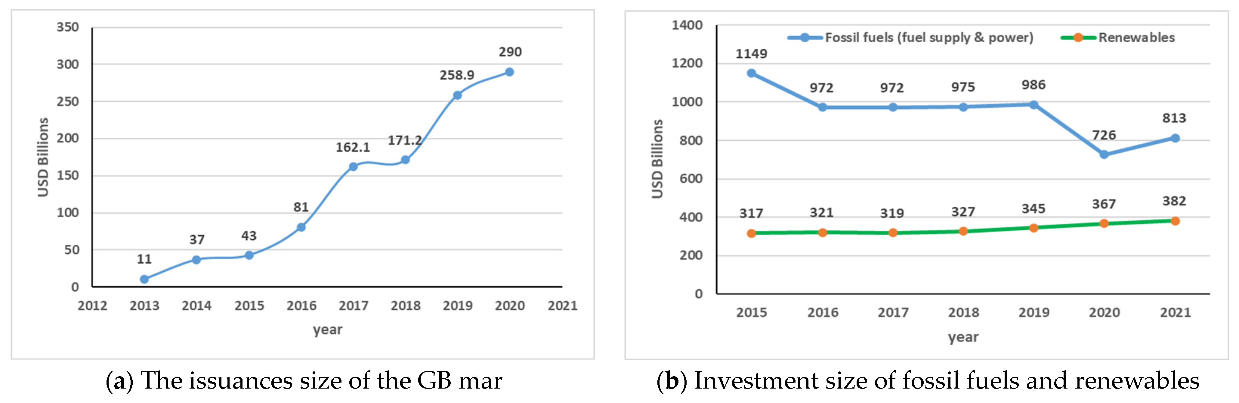
To mitigate the environmental degradation caused by climate change, environmentally conscious investors and policymakers have shown increased interest in investing in green development. As shown in Figure 1b, over 2015–2021, investments for building new renewable capacity through traditional financing, such as shares and corporate bonds, showed a slow upward trend from USD 317 bn in 2015 to USD 382 bn in 2021, while investments in fuel supply and power showed a downward trend from USD 1149 bn in 2015 to USD 813 bn in 2021. However, the amount invested in the fossil fuel market is still higher than that invested in renewable energy.

Green bonds (GBs) are financial instruments that are aimed at mitigating adverse environmental impact through the investment of financial assets in renewable energy projects. GBs are relatively new fixed-income assets, and their proceeds are generally used for environmental projects geared toward mitigating climate change (Reboredo, 2018 [2]). Although GBs represent less than 1% of the bond market (Reboredo, 2018 [2]), the scale of investment in GBs is growing rapidly. As the amount of GBs issued showed a growing trend from USD 11 bn in 2013 to USD 290 bn in 2020 (see Figure 1a), GBs are expected to develop further and help mobilize the financing needed to improve renewable capacity and energy efficiency.

Thus, understanding how the GB market relates to clean energy (CE) stock and fossil fuel markets can offer essential information for energy investors and policymakers to identify the importance of the GB markets. This information would demonstrate how GB markets prices may be impacted by price oscillations in the energy markets. If there is a strong relationship between GBs and CE and the fossil fuel market, then the GB markets may affect or be affected by CE and fossil fuel markets. This implies the significance of considering the mutual effect among GB, CE, and fossil fuels when developing policies and investing in efforts to improve the areas of energy conversion.

Moreover, volatility spillover is defined as the transmission of instability from market to market. It occurs when the volatility price change in one market causes a lagged impact on the volatility price in another market above the local effects of the market, which is important information for understanding the transmission of the price volatility risk between the two markets. Thus, understanding the volatility spillover among GBs, CE, and fossil fuels may help policymakers deal with the price volatility risk involved in developing the GB markets. If the changes in the CE and fossil fuel prices also lead to volatility in GB prices, then policymakers need to use appropriate policy instruments to eliminate the risk of the price volatility spillover effects of CE and fossil fuel on GB markets and thereby ensure issuance price stability. It is particularly important to assure investors of GB yields, which are crucial in mobilizing the financing needed for sustainable investment (Reboredo and Ugolini, 2020 [3]).

Prior studies have documented evidence supporting the spillover effects between the GBs and equity markets (Pham, 2021 [4] ), and the relationship between GBs and the energy commodity index (Reboredo, 2018 [2]; Reboredo and Ugolini, 2020 [3]). However, the inadequate samples of specific prices of fossil fuel (e.g., coal, West Texas Intermediate (WTI) oil, Brent oil (Brent), natural gas (NG)) and the inappropriate methodologies have restricted the validity and generalizability of the findings for analyzing the short-term, medium-term, and long-term investment horizons.

To expand previous research (Reboredo, 2018 [2]; Reboredo and Ugolini, 2020 [3]; Pham 2021 [4]), the current study examines how the GB market is related to CE stocks and fossil fuel markets (coal, WTI, NG, etc.) simultaneously by applying the Bayesian dynamic conditional correlation (DCC) multivariate generalized autoregressive conditional heteroskedasticity (MGARCH) model. Furthermore, we study how the volatility spillover effects among these markets change in the short-term, medium-term, and long-term horizons by using the frequency connectedness method developed by Baruník and Křehlík (BK method hereafter) (2018) [5]. Based on the results of the above two studies, our goal is to propose sustainable investment recommendations to investors or policymakers who want to identify the importance of the GB markets and deal with the price volatility risk involved in developing the GB markets.

In this study, we focus on the US markets, which remain the largest source of green debt, with a total of USD 52.1 bn (18%) (Climate Bonds Initiative, 2020 [6]), and the world’s largest energy and financial trading markets. With these characteristics, the US market can effectively reflect the co-movement of the GB markets with the CE stock and fossil fuel markets. Meanwhile, we consider Brent crude oil in identifying the impact of crude oil on GBs, as this oil type is the most volatile of the fossil fuel products.

This study offers two important contributions. First, it analyzes the changes in the volatility spillover effects among GBs, CE, and fossil fuels in the short-term, medium-term, and long-term horizons for investors or policymakers to identify the price volatility spillover risk of another energy market on GB markets from a frequency perspective to achieve sustainable investment. Second, it introduces a new method that combines the Bayesian DCC-MGARCH model (Tang and Aruga, 2022 [7]) and frequency connectedness method (BK, 2018 [5]) to analyze the new GB market in relation to the CE and fossil fuel markets to gain more dynamic information, such as a dynamic correlation and frequency volatility spillover between them. Firstly, the Bayesian DCC-MGARCH model is sampled by Monte Carlo simulation, which makes the prediction of dynamic relations among GB, CE, and fossil fuel markets more flexible and less biased, because the Monte Carlo simulation can overcome the problem of the maximum likelihood method being difficult to fit on wider parameter regions, and then estimate in the wider parameter region to obtain more information. Secondly, the frequency connectedness method uses the frequency impulse function variance decomposition method to decompose the structure of volatility spillover into short-term, medium-term, and long-term horizons, which can provide more dimensional information for investors and policymakers.

The rest of the paper is structured as follows. Section 2 presents a review of the existing literature. Section 3 and Section 4, respectively, describe the data and methods used in this study. Section 5 covers the results of the analysis and the relevant discussion. Section 6 provides a summary of the conclusions.

2. Previous Research

Some previous empirical research has attempted to review the GB market by using extensive literature and market data analysis (Ehlers and Packer, 2017 [8]; Banga, 2018 [9]; MacAskill et al., 2021 [10]; etc.). Ehlers and Packer (2017) [8] examined the certification of GB financing and suggested that more consistent GBs across jurisdictions could help the market to further develop because a standard certification makes it easier for asset managers to identify environmentally related financial risks. Banga (2018) [9] explored the drivers and barriers of the GB market relative to conventional bonds for developing countries, reporting that some of the barriers include the lack of appropriate institutional arrangements for GB management, which leads to the issue of minimum size, and the high transaction costs associated with GB issuance; meanwhile, the key drivers include investors’ increasing climate awareness. As for the premium of the GB market, Macaskill et al. (2021) [10] suggested that GBs have a 56% and 70% green premium when issued in the primary and secondary markets, respectively, and concluded that the environmental preferences of investors should be considered in future bond pricing.

Other studies have focused on how GBs differ from traditional bonds (Pham, 2016 [11]; Zerbib, 2017 [12]; Zerbib, 2019 [13]; Nanayakkara and Colombage, 2019 [14]; Lebelle et al., 2020) [15]. Pham (2016) [11] suggested that the impact of a shock on the entire conventional bond market may spill over into the GB market and with the spillover effect being time-varying. Zerbib (2017) [12] employed a matching method to survey the GB premium relative to 135 investment-grade senior bullet fixed-rate GBs and reported that the difference in yield between a GB and a conventional bond is controlled by the difference in liquidity between the two bonds. Moreover, Zerbib (2019) [13] suggested that the yield of GB has a small negative premium that is lower than that of a conventional bond. As GBs have a lower negative premium, they are important for funding to achieve sustainable development (Nanayakkara and Colombage, 2019 [14]). However, Lebelle et al. (2020) [15] suggested that the investors react in the same manner as GBs are no different from conventional or convertible bonds.

From the perspective of investors, the factors affecting the GB market are important for its development. Pham and Luu Duc Huynh (2020) [16] used the vector autoregressive (VAR) model to identify how the factor of investor attention is related to GB growth, and explained that the link between them varies over time and is stronger in the short run than in the long run. The mechanism of influence of investor sentiment on the GB markets was studied by Piñeiro-Chousa et al. (2021) [17], who suggested that investor sentiment has a positive impact on GBs’ returns. Other macroeconomic latent factors (regulatory quality, the rule of law, stock market capitalization, size of the economy, and trade openness) also positively affect the development of GB markets (Tolliver et al., 2020 [18]). For example, the macroeconomic factors related to infrastructure and the economy contribute to the development of the GB markets in Vietnam (Tu et al., 2020 [19]). In addition, Broadstock and Cheng (2019) [20] suggested that changes in the connection between GBs and black bonds are influenced by macro factors such as economic policy uncertainty, financial market volatility, and daily economic activity.

For portfolio investment and risk management, the work of Reboredo (2018) [2], Reboredo and Ugolini (2020) [3], Tiwari et al. (2022) [21], Dutta et al. (2021) [22], Lee et al. (2021) [23], and Pham (2021) [4] studied the co-movement among the GB and other markets. Reboredo (2018) [2] employed the threshold GARCH model to show that the co-movement between the GB market and the energy commodity index is not significant, although the GB markets are affected by substantial price spillovers from traditional bonds. Reboredo and Ugolini (2020) [3] used the structural VAR model to determine the connectedness between the GB and energy markets (S&P GSCI Energy spot), and reported that high-yield corporate bond markets are relatively weak. In addition, Dutta et al. (2021) [22] employed the VAR-asymmetric DCC-GARCH model to identify that the dynamic correlations among GB, stock, gold, and the oil market is switching between positive and negative states. Lee et al. (2021) [23] suggested a significant bi-directional causality from oil price to the GB index. Tiwari et al. (2021) [21] studied the transmission of return patterns between GB, carbon prices, and renewable energy stocks by using the time-varying parameter (TVP)-VAR approach, and found that when a shock occurs, the GB and wind indexes are the main net recipients of the solar and S&P CE index, which is the main net transmitter of shocks. Moreover, Pham (2021) [4] used the frequency connectedness method to suggest that the spillover effects between GBs and green equity are significant in the short term, and dissipate in the medium- and long-term investment horizons.

Finally, due to the occurrence of COVID-19, there are some studies on the associations between green bonds and commodity prices. For example, Rehman et al.(2023) [24] employ the OLS predictive model to examine the predictive power of oil shocks for the green bond markets in the period classifying the dataset into pre-COVID-19 and COVID-19 eras, and the results show that the oil shocks have predictive power for green bonds during the crisis period. Su et al. (2023) [25] used the quantile-on-quantile (QQ) method to investigate how oil prices influence the prospects of green bonds during the COVID-19 period, and found that the impacts of oil prices on green bonds are positive in the short run. Wang et al. (2022) [26] only investigated the link between crude oil prices and green bonds using the Granger-causality test, and showed that green bonds could not moderate the oil crisis due to COVID-19, instability in the international political environment, and the immaturity of the green bond market. In addition, there are some other perspective studies on the associations between green bonds and gas prices. For example, the volatilities and conditional correlations between green bonds and US gas prices are investigated by Abakah et al. (2023) [27], who use GO-GARCH, ADCC, and DCC models to evidence that green bonds have a strong correlation with shale gas and natural gas.

However, the above studies only focus on the impact of an energy market (such as oil or natural gas prices) on green bonds, but lack the consideration of the impact of coal and clean energy on green bonds. This will lead to losing some useful information for analyzing the impact of the entire energy market on the green bond market. At the same time, only COVID-19 factors are considered to investigate the relationship between energy and green bonds; this will also lose other useful information. For example, there is information on the impact of other political events factors, such as the OPEC agreement and the Russia–Ukraine War, which occurred during COVID-19. In order to avoid the influence of other factors, unlike in other studies, we focus on the price based on Fama’s efficient market hypothesis (Fama, 1991) [28], assuming that the demand and supply factors are incorporated in the market price, and our study will further examine the dynamic correlation and volatility spillover among GBs, CE stocks, and fossil fuel markets (coal, WTI, NG, etc.) simultaneously using the Bayesian DCC-MGARCH model and frequency connectedness method.

3. Data

This section may be divided into subheadings. It should provide a concise and precise description of the experimental results, their interpretation, as well as the experimental conclusions that can be drawn.

To explore the dynamic correlation and risk spillover effects among the GBs, fossil fuel, and CE markets, we consider the daily data of the S&P U.S. Municipal GB Index, the fossil fuel market (coal, WTI, Brent, Henry Hub NG, heating oil (HO), and gasoline), and Invesco Wilder Hill CE Index as samples analyzed in this study from 30 June 2014 to 18 October 2021.

(1) S&P U.S. Municipal GB Index. This index is designed to track the U.S. green municipal bond market. It is more representative of the green-labeled bonds index because it maintains stringent standards and includes only those bonds whose proceeds are used for financing environmentally friendly projects, such as those that promote climate change mitigation and other environmental sustainability efforts. The index is developed by the institutions of S&P Dow Jones Indices and calculated in USD on the basis of its fixed income policies and practices methodology. Thus, the index is sourced from the S&P Dow Jones Indices (2021) [29].

(2) Fossil fuel market. These samples included coal (USD/ton), WTI (USD/barrel), Brent (USD/Barrel), Henry Hub NG (USD/MMBtu), HO (USD/100 L), and gasoline (USD/gallon) commodity prices, which were obtained from INSIDER (2021) [30]. The official daily close prices are last traded at a particular trading time; thus, we used them as representative benchmark prices of daily trading for each of the fossil fuel markets.

(3) Invesco Wilder Hill CE Index. As this CE Index is not directly available, we used the CE exchange-traded fund as a proxy variable because it is based on the CE index. The daily prices of the index are computed on the basis of the stocks of U.S. publicly traded companies engaging in the business of advancing CE and conservation sourced from Invesco (2021) [31].

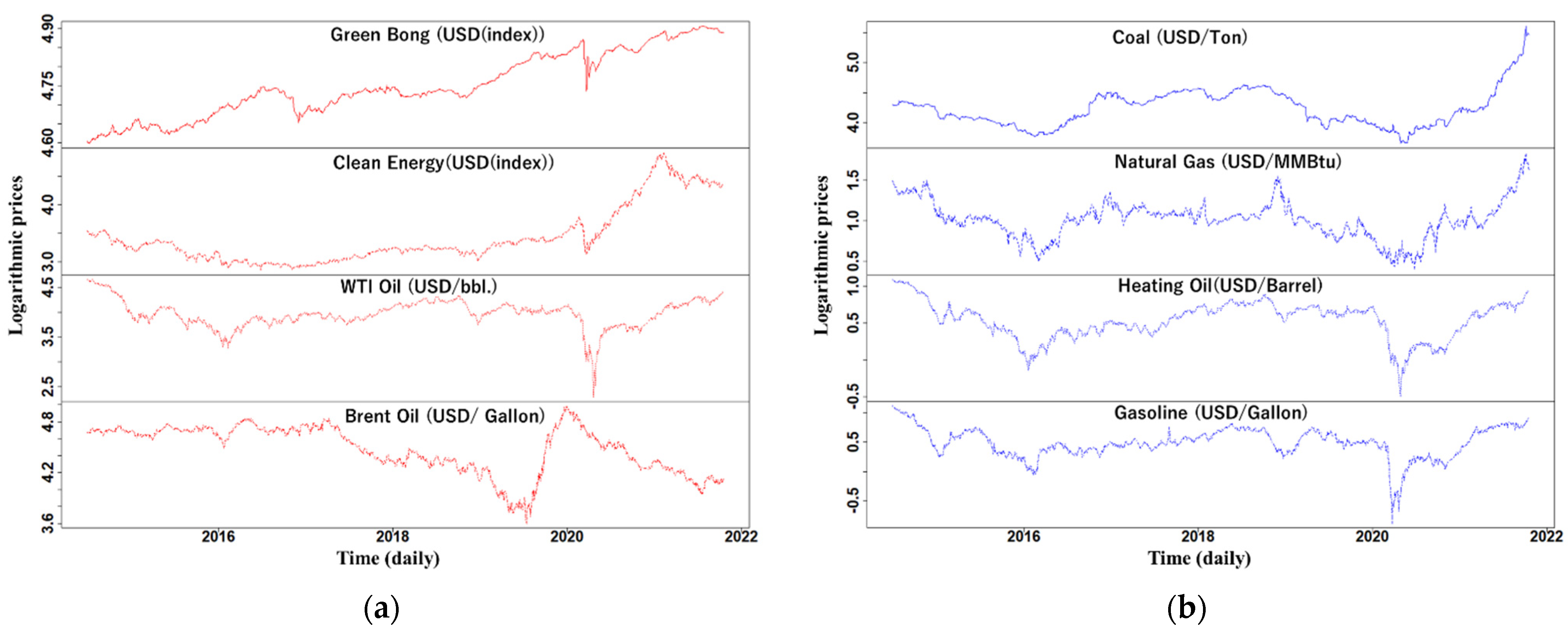
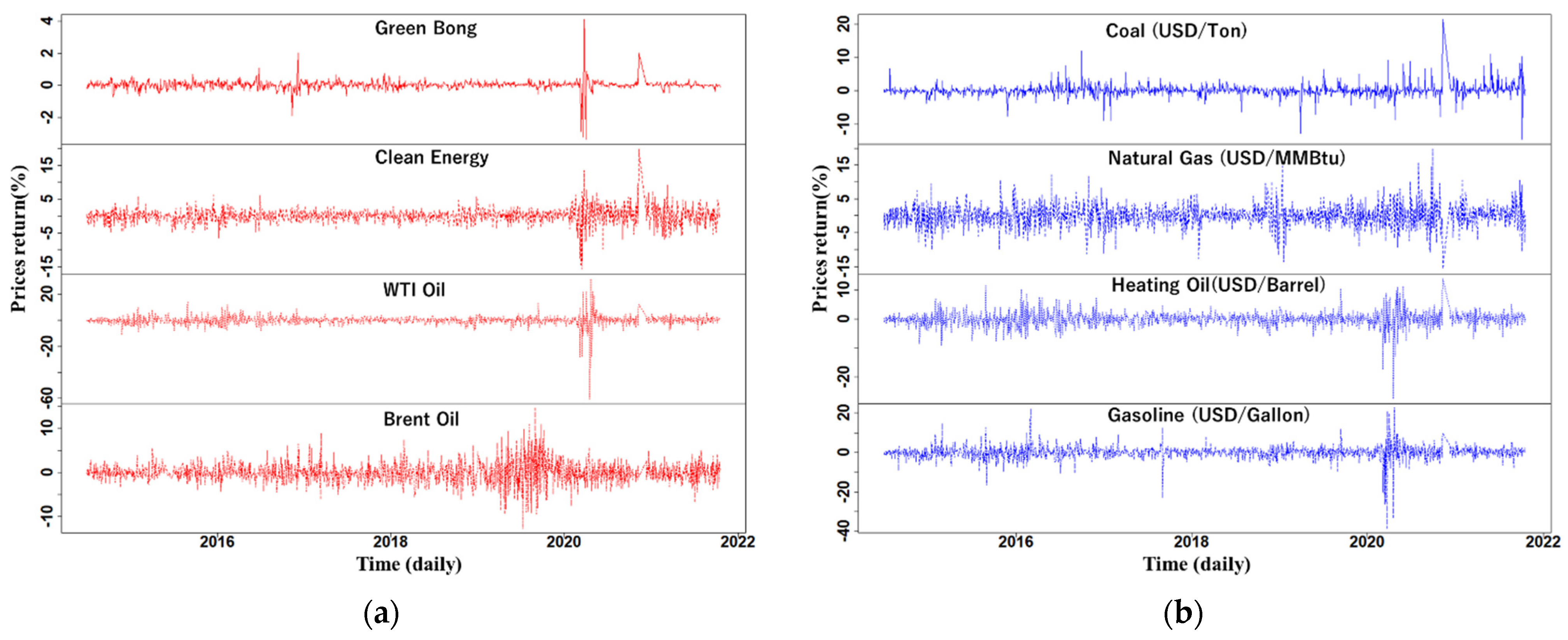
As the samples mentioned above have different calculation units, we denote them uniformly as logarithms, as shown in Figure 2. In addition, the frequency connectedness method and DCC-MGARCH model need to use price return data; thus, the percentage of continuously compounded returns $r_t$ is computed by $r_t$ = 100 × [ln($p_t$) − ln($p_{t-1}$)], where $p_t$ denotes the GB, fossil fuel, and CE prices in period t. Figure 3 reports the plot of price returns against time.

4. Methods and Materials

It is known that the Bayesian DCC-MGARCH model is flexible for capturing the dynamic correlation between fossil fuels and the financial market (Tang and Aruga, 2022 [7]). As the shocks to economic activity impact variables at various frequency domains with various strengths, we applied the frequent domain spillover approach of BK (2018) [5], which overcomes the hypothesis that the preferences, anticipations, expectations, and risk aversion of the market participants are the same, which is ignored by Diebold and Yilmaz (DY method hereafter) (2012) [32].

Thus, we first discuss the methodology of the Bayesian DCC-MGARCH model to analyze the correlation between GBs, CE, and fossil fuels. We secondly elaborate on the frequency-domain spillover methods of BK (2018) [5] for different market participants to identify which market among GBs, CE, and fossil fuels is the spillover or the recipient of price volatility and to estimate how the extent of the volatility spillover among them are changing at short-, medium-, and long-term investment horizons.

4.1. Bayesian DCC-MGARCH Models

In the Bayesian DCC-MGARCH model framework, we follow the framework of Tang and Aruga (2022) [7] for discussion.

First, the conditional correlation can be obtained from the decomposition of the conditional covariance matrix because of the conditional heteroskedasticity in the MGARCH model. If the conditional correlation matrix is time-invariant, then it is called a constant conditional correlation (CCC) matrix. However, the most empirical applications (Dutta et al., 2021 [22]; Shiferaw, 2019 [33]; Tang and Aruga, 2022) [7] showed that the hypothesis of a CCC matrix is not very realistic and the dynamic conditional correlation (DCC) is more flexible by allowing the conditional correlation matrix to be time-varying. Therefore, we applied the DCC-MGARCH model, and it can be made up of the following equations:

$$P_t={\mu }_t+r_t$$

(1)

$$r_t=H_t{}^{1/2}{Z}_t$$

(2)

$$H_t=D_t{R}_t{D}_t$$

(3)

$$D_t=diag \left(h_{11t}{}^{\frac{1}{2}}\dots h_{nnt}{}^{\frac{1}{2}}\right)$$

(4)

$$R_t=\{diag{\left(Q_t\right)}^{\frac{1}{2}}\}{Q}_t\{diag{\left(Q_t\right)}^{\frac{1}{2}}\}$$

(5)

where $P_t$ is a vector of the logarithmic value of the GB, fossil fuel, and CE market price at time $t$. ${\mu }_t$ is a vector of the expected value of $P_t$. $r_t$ is a vector of the returns related to $P_t$ asset prices at time $t$ with $E\left[r_t\right]$ = 0, $\mathrm{Cov}[r_t]$ = $H_t$, E($Z_t$) = 0, and $E\left(Z_t{Z}_t{}^{\prime }\right)$ = $I$. $H_t$ and $Z_t$ are conditional variance matrix and identically independently distributed ($iid$) errors, respectively. $D_t$ is a diagonal matrix of standard deviations, including the conditional covariance $h_{nnt}{}^{\frac{1}{2}}$. $R_t$ is the time-varying correlation matrix, including the symmetric positive definite matrices $Q_t$ = (${\rho }_{ij,t}$).

Given a GARCH (p, q) model for each conditional covariance $h_{ii,t}$ and symmetric dynamic correlation $R_t$, they are specified as follows:

$$h_{ii,t}={\omega }_i+{{\displaystyle \sum }}_{p=1}^{P_i}{\alpha }_{ip}{r}_{i,t-p}^2+{{\displaystyle \sum }}_{q=1}^{Q_i}{\beta }_{iq}{h}_{ii,t-q},i=1, 2, \dots , n$$

(6)

$$Q_t=\left(1-a-b\right)\overline{Q}+a{ϵ}_{t-1}{ϵ}_{t-1}^{\prime }+b{Q}_{t-1}$$

(7)

$$R_t=Q_t^{*-1}{Q}_t{Q}_t^{*-1}$$

(8)

where ${\omega }_i>0,{\alpha }_i\ge 0,{\beta }_i\ge 0,{\displaystyle \sum }_{q=1}^{Q_i}{\alpha }_{iq}+{\displaystyle \sum }_{p=1}^{P_i}{\beta }_{ip}<1$. In addition, $\overline{Q}$ is the unconditional covariance matrix computed by $Cov\left[{ϵ}_t{ϵ}_t^{\prime }\right]=E\left[{ϵ}_t{ϵ}_t^{\prime }\right]$, where ${ϵ}_t$ is the standardized error. To ensure positive unconditional variances, the parameters $a$ and $b$ are $a\ge 0$, $b\ge 0$, and $a+b<1$. The $Q_t^{*}$ is the diagonal matrix with the square root of the diagonal elements of $Q_t$. For a detailed equation, please see Tang and Aruga (2022) [7].

Next, we applied the Bayesian approach to estimate the parameters of the DCC-MGARCH model. Due to financial time series data often being skewed (Fioruci, Ehlers, and Filho, 2014 [34]), we consider three different innovation distributions: skew multivariate normal (SMN) with a shape parameter $\gamma$, skew multivariate Student t (SMST) with an extra parameter $\nu$, and skew multivariate generalized error distribution (SMGED) with a tail parameter $\delta$. For a detailed equation, please see Tang and Aruga (2022) [7].

If the SMN is assumed to calculate the error $Z_t$ in Equation (2), the extra parameter $\nu$ is not needed to be estimated. However, the SMST is considered to be an error $Z_t$, given the extra parameter $\nu$ to SMN. Additionally, if the error $Z_t$ are SMGED, another the extra parameter $\delta$ will be calculated. Therefore, parameter $\theta =\left({\omega }_i,{\alpha }_i,{\beta }_i,\nu ,\delta ,{\gamma }_i,a,\mathrm{b}\right)$ is needed to set the prior distributions for estimating these parameters based on the Bayesian theory. For setting prior distributions, please see Tang and Aruga (2022) [7].

Finally, according to Fioruci, Ehlers, and Filho (2014) [34] and Tang and Aruga (2022) [7], the Markov chain Monte Carlo (MCMC) method was used to sample the joint posterior distributions from the prior distributions, and the Metropolis–Hastings algorithm is applied to provide the easiest sampling. In addition, the Akaike Information Criterion (AIC), Bayesian Information Criterion (BIC), and Deviance Information Criterion (DIC) are applied to choose the best DCC-MGARCH model. The best-fitting model can be judged by the minimum value of the AIC, BIC, and DIC.

4.2. The Frequency-Domain Spillover Methods

Due to the DCC-MGARCH model not allowing for calculating the volatility spillover, we used the frequency-domain spillover methods by decomposing variance from a vector autoregressive (VAR) model. This measuring is how BK (2018) [5] imported a set of frequency domains into the generalized forecast error variance decompositions (GFEVD) of DY (2012) [32] to explore short-, medium-, and long-term volatility spillover. Hence, we first discussed the method of DY (2012) [32] and then defined the connectedness measures in the frequency domain of BK (2018) [5].

4.2.1. Measuring Connectedness with Variance Decompositions

Given n-variate process $x_t=\left(x_{t1},\dots , x_{tn}\right), t=1\dots .T$, the mathematical representation of the VAR(p) is written as follows:

$$x_t={\varphi }_0+{\displaystyle \sum }_{i=1}^p{\varphi }_i{x}_{t-i}+{\epsilon }_t$$

(9)

where $x_t$ is a vector of the $k$ price series of this study. ${\varphi }_0$ is a constant vector ($k\times 1$), ${\varphi }_1\cdots {\varphi }_n$ are coefficient matrices to be estimated ($k\times k$), $p$ is the optimal lag order, and the model with the lower value of Schwarz information criterion (SIC) is preferred for selecting optimal lag. The ${\epsilon }_t\sim \left(0,\Sigma \right)$ is a vector of $i.i.d$ disturbances with covariance matrix $\Sigma$.

Following DY (2012) [32], given the assumption of stationary covariance, the VAR process has a vector moving average (i.e., MA ($\infty$)) as follows:

$$x_t={\displaystyle \sum }_{i=0}^{\infty }{\psi }_i{\epsilon }_{t-i}$$

(10)

where ${\displaystyle \sum }_{i=0}^{\infty }{\psi }_i=\psi \left(L\right)$ is a matrix of infinite lag polynomials calculated by $\varphi \left(L\right)={\left[\psi \left(L\right)\right]}^{-1}$. Moreover, the GFEVD can be written as follows:

$${\left({\Theta }_H\right)}_{ij}=\frac{{\sigma }_{jj}^{-1}{{\displaystyle \sum }}_{h=0}^H({\left({\psi }_h\Sigma {)}_{ij}\right)}^2}{{{\displaystyle \sum }}_{h=0}^H{({\psi }_h\Sigma {\psi }_h^{\prime })}_{jj}}$$

(11)

where ${\psi }_h$ is a ($N\times N$) matrix of moving average coefficients at lag $h$, and ${\sigma }_{jj}={(\Sigma )}_{jj}$. The term ${\left({\Theta }_H\right)}_{ij}$ is denoted as the contribution of the $j$-th variable to the variance of the forecast error of $i$-th variable at forecast horizon $H$. Since the values of the corresponding rows of the variance decomposition matrix ${\Theta }_H$ do not sum to 1, we normalize them by the row sum as follows:

$${\left({\tilde{\Theta }}_H\right)}_{ij}=\frac{{\left({\Theta }_H\right)}_{ij}}{{{\displaystyle \sum }}_{i=1}^N{\left({\Theta }_H\right)}_{ij}}$$

(12)

where ${\displaystyle \sum }_{i=1}^N{\left({\tilde{\Theta }}_H\right)}_{ij}=1$ and the sum of all elements in the structure of ${\tilde{\Theta }}_H$ is equal to $N$. In addition, the pairwise connectedness from the $j$-th variable to $i$-th variable is measured by ${\left({\tilde{\Theta }}_H\right)}_{ij}$ at forecast horizon $H$.

4.2.2. Frequency Response Function for Decomposing Variance

For measuring connectedness in the frequency domain (short, medium, long-term), the spectral representation of variance decompositions based on frequency responses to shocks instead of impulse responses to shocks needs to be considered (BK, 2018 [5]). If the coefficients ${\psi }_i$ in Equation (9) made the Fourier transformation, a frequency response function is obtained as follows:

$$\psi \left(e^{-i\omega }\right)= {\displaystyle \sum }_h{e}^{-i\omega h}{\psi }_h$$

(13)

where $w$ implies frequency and $i=\sqrt{-1}$.

Given a frequency $w$, the spectral density of $x_t$ in Equation (9) can be expressed as follows:

$$S_x\left(\omega \right)={\displaystyle \sum }_{h=-\infty }^{\infty }E\left(x_t{x}_{t-h}^{\prime }\right)e^{-i\omega h}={\psi }_h\left(e^{-i\omega }\right)\Sigma {\psi }^{\prime }\left(e^{+i\omega }\right)$$

(14)

where $S_x\left(\omega \right)$ is the power spectrum that can be used for identifying how the variance of the $x_t$ is distributed over the frequency components $\omega$.

Moreover, according to the “Definition 2.1” of BK (2018) [5], the generalized causation spectrum over frequencies $\omega \in \left(-\pi ,\pi \right)$ is given by the following:

$${\left(f\left(\omega \right)\right)}_{ij}=\frac{{\sigma }_{jj}^{-1}{\left({\left(\psi \left(e^{-i\omega }\right)\Sigma \right)}_{ij}\right)}^2}{{\left(\psi \left(e^{-i\omega }\right)\Sigma {\psi }^{\prime }\left(e^{+i\omega }\right)\right)}_{ii}}$$

(15)

where $\psi \left(e^{-i\omega }\right)$= ${\displaystyle \sum }_h{e}^{-i\omega h}{\psi }_h$, ${\left(f\left(\omega \right)\right)}_{ij}$ is the portion of the spectrum of the $i$-th variable at frequency $\omega$ that results from the shock to the $j$-th variable. As the denominator holds the spectrum of the $i$-th variable, which is on the diagonal element of the cross-spectral density of $x_t$ at frequency $\omega$, we thus can interpret the ${\left(f\left(\omega \right)\right)}_{ij}$ as within-frequency causation. To obtain a natural decomposition of the GFEVD to frequencies, we used the frequency share of the variance of the $i$-th variable to weight ${\left(f\left(\omega \right)\right)}_{ij}$. The weighting function is defined as follows:

$${\Gamma }_i\left(\omega \right)=\frac{{\left(\psi \left(e^{-i\omega }\right)\Sigma {\psi }^{\prime }\left(e^{+i\omega }\right)\right)}_{ii}}{\frac{1}{2\pi }{{\displaystyle \int }}_{-\pi }^{\pi }{\left(\psi \left(e^{-i\lambda }\right)\Sigma {\psi }^{\prime }\left(e^{+i\lambda }\right)\right)}_{ii}d\lambda }$$

(16)

where ${\Gamma }_i\left(\omega \right)$ is the power of the $i$-th variable at a given frequency $\omega$ whose sum is to be a constant value of $2\pi$. Given a frequency band $d=\left(a,b\right)$, the GFEVD at a frequency band $d$ is defined as follows:

$${\left({\Theta }_d\right)}_{ij}=\frac{1}{2\pi }{{\displaystyle \int }}_a^b{\Gamma }_i\left(\omega \right){\left(f\left(\omega \right)\right)}_{ij}d\omega$$

(17)

where $a$, $b$ $\in \left(-\pi ,\pi \right)$, $a$ < $b$.

Firstly, the decomposition in Equation (17) is used to obtain within-total, pairwise, and net connectedness at the band $d$. The within-total connectedness is important for us to identify the connectedness effect occurring within the frequency band. The pairwise connectedness is variance transmission from one market to another market. The net connectedness is variance transmission from another market to one market that is a net giver/receiver of variance to/from all other markets if the net connectedness is a positive/negative value. For a detailed decomposition, please see “Definition 2.2” of BK (2018) [5].

4.2.3. Estimation of Connectedness in the Frequency Bands

For exploring short-, medium-, and long-term volatility spillover, we set eight frequency bands: d1({2–4} days), d2({4–8} days), d3({8–16} days), d4({16–32} days), d5({32–64} days), d6({64–128} days), d7({128–256} days), and d8({256–512} days) based on the work of Mensi et al. (2021) [35]. Moreover, according to Maghyereh et al. (2019) [36], the sum of the d1 and d2 series is defined as the short-term horizon equivalent to the periods 2 days to 8 days. The medium-term horizon is the sum of d3 and d4, corresponding to the periods 8 days to 32 days. In addition, we assumed that the long-term horizon is the sum of d5 to d8, corresponding to the periods 32 days to 512 days based on Mensi et al. (2021) [35] and Maghyereh et al. (2019) [36]. We estimated the connectedness on desired frequencies by R 4.5 soft. The codes come from the “frequencyconnectedness-package” of Barunik and Krehlik (2018) [5] and the “bayesDccGarch-Package-Package” of Fiorucci et al. (2014) [34]. For detailed computations, please see the links in the “Supplementary Material”.

4.3. Variable Characteristics

Before identifying the correlation and volatility spillover among GBs, CE, and fossil fuels, we need to understand the statistical characterization of our test variables. First, we applied the Augmented Dickey–Fuller (ADF), Phillips–Perron (PP), and Kwiatkowski–Phillips–Schmidt–Shin (KPSS) tests to test the stationarity of our test variables to avoid pseudo-regression problems. Second, the Shapiro–Wilk (SW) and Jarque–Bera (JB) tests are used to detect the normality, skewness, and kurtosis of the sample distribution. Moreover, we applied Engle’s Lagrange multiplier (LM) test to identify the effects of autoregressive conditional heteroscedastic (ARCH) for each of the returns.

5. Result

5.1. Descriptive Summary of All Prices and Return Series Data

Table 1. Unit root tests.

Variables	Level Data (t-Value)						First Difference Data
	ADF	PP	KPSS	ADF	PP	KPSS	ADF	PP	KPSS
	(Return)	(Return)	(Return)	(Price)	(Price)	(Price)	(Price)	(Price)	(Price)
GB	−11.28 *	−22.77 *	0.02	−3.18	−3.27	16.60 *	−11.28 *	−22.42 *	0.02
	(0.01)	(0.01)	(0.10)	(0.09)	(0.08)	(0.01)	(0.01)	(0.01)	(0.10)
CE	−11.36 *	−40.18 *	0.43	−1.93	−1.80	9.27 *	−10.93 *	−39.03 *	0.24
	(0.01)	(0.01)	(0.06)	(0.61)	(0.66)	(0.01)	(0.01)	(0.01)	(0.10)
Coal	−10.97 *	−34.84 *	0.86 *	4.98	4.26	1.64 *	−10.20 *	−36.88 *	1.22 *
	(0.01)	(0.01)	(0.01)	(0.99)	(0.99)	(0.01)	(0.01)	(0.01)	(0.01)
WTI	−11.53 *	−41.91 *	0.21	−2.80	−2.75	0.93 *	−10.60 *	−41.53 *	0.56 *
	(0.01)	(0.01)	(0.10)	(0.24)	(0.26)	(0.01)	(0.01)	(0.01)	(0.03)
Brent	−11.08 *	−43.60 *	0.08	−1.98	−1.91	6.82 *	−11.00 *	−42.30 *	0.08
	(0.01)	(0.01)	(0.10)	(0.59)	(0.62)	(0.01)	(0.01)	(0.01)	(0.10)
NG	−11.81 *	−40.76 *	0.24	−2.02	−2.09	1.11 *	−10.89 *	−41.38 *	0.31
	(0.01)	(0.01)	(0.10)	(0.57)	(0.54)	(0.01)	(0.01)	(0.01)	(0.10)
HO	−11.21 *	−41.51 *	0.28	−2.17	−2.17	1.07 *	−11.12 *	−41.72 *	0.51 *
	(0.01)	(0.01)	(0.10)	(0.51)	(0.51)	(0.01)	(0.01)	(0.01)	(0.04)
Gasoline	−10.39 *	−42.40 *	0.18	−2.80	−2.85	0.93 *	−10.31 *	−42.00 *	0.41
	(0.01)	(0.01)	(0.10)	(0.24)	(0.22)	(0.01)	(0.01)	(0.01)	(0.07)

Note: * Denotes statistical significance at the 5% level. Heating oil: HO; natural gas: NG.

presents the results of the ADF, PP, and KPSS test results, indicating that all price series data are non-stationary at a 5% level of significance, but become stationary when first differencing them. In addition, all the return series are stationary at a 5% level of significance.

Table 2. Statistical properties of fossil fuel, CE, and GB market returns.

Variables	Max.	Min.	Std.	Skewness	Kurtosis	JB	SW	LM
GB	4.13	−3.38	0.29	−0.74	67.74	307,810 **	0.61 **	2077.02 **
						(0.00)	(0.00)	(0.00)
CE	19.84	−15.64	2.21	−0.12	9.68	6290 **	0.91 **	1352.33 **
						(0.00)	(0.00)	(0.00)
Coal	21.51	−14.65	1.72	1.33	27.83	52,417 **	0.74 **	9780.68 **
						(0.00)	(0.00)	(0.00)
WTI	31.96	−60.17	3.60	−2.66	62.09	260,387 **	0.73 **	4094.26 **
						(0.00)	(0.00)	(0.00)
Brent	14.57	−12.71	2.30	0.31	4.04	1278 **	0.96 **	1015.08 **
						(0.00)	(0.00)	(0.00)
NG	19.80	−15.77	3.18	0.14	3.19	2553 **	0.95 **	1484.11 **
						(0.00)	(0.00)	(0.00)
HO	13.95	−27.43	2.46	−0.79	14.07	6028 **	0.90 **	3397.69 **
						(0.00)	(0.00)	(0.00)
Gasoline	22.40	−38.54	3.31	−1.78	27.79	307,810 **	0.61 **	4070.25 **
						(0.00)	(0.00)	(0.00)

Note: ** Denotes statistical significance at the 1% level. Heating oil: HO; natural gas: NG.

shows the results of the summary statistics. The JB test results suggested that all the return series have skewness and excess kurtosis at the 1% level. The SW test results indicated the null hypothesis of a normally distributed population is rejected at a 1% level of significance in each of the return series. All of the JB and SW test results highlight the validity of considering asymmetric distributions instead of normal distributions. Moreover, the LM test results suggested that all return series have the ARCH effects at a 1% level of significance. These results imply the need to consider the three different innovation distributions introduced in Equations (9)–(11) for fitting the Bayesian DCC-MGARCH (1,1) models.

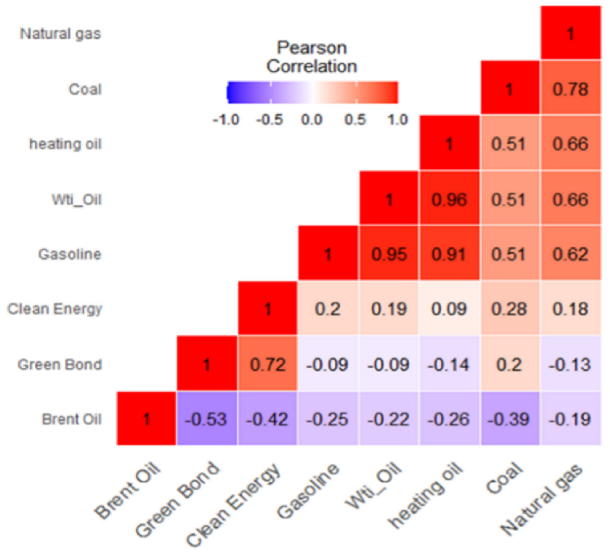
Figure 4 shows the heat map of a visual correlation matrix across the GB, CE, and fossil fuel assets. The magnitude of the correlation is indicated by the color intensity of the shaded boxes, and the red color shows a positive correlation, while the blue color presents a negative correlation. The map shows a strong positive correlation between WTI, coal, NG, HO, and gasoline, but a negative correlation is observed between Brent and other market assets. It would be worthwhile to note that GBs have a negative correlation with WTI, NG, HO, and gasoline, and a positive correlation with coal and the CE stock market.

5.2. Bayesian Estimation of the DCC-MGARCH (1,1) Model

For estimating parameter $\theta =\left({\omega }_i,{\alpha }_i,{\beta }_i,\nu ,\delta ,{\gamma }_i,a,\mathrm{b}\right)$, we use the MCMC method to run 10,000 iterations with a burn-in phase of 1000 and a thinning interval of 10 to sample the posterior distribution following Fioruci, et al.,(2014) [34]. The first 1000 samples were rounded off, and the remaining 9000 samples were kept for estimating each parameter sample.

Table 3. Information criteria for all returns under the SMN, SMST, and SMGED.

	Cri.	SMN	SMST	SMGED
All return	AIC	44,566.8	42,716.43	42,611.94
	BIC	44,749.75	42,904.76	42,800.27
	DIC	44,571.85	42,709.34	42,644.03

Notes: All returns included the GB, CE, Brent, WTI, Coal, NG, HO, and Gasoline.

displays the results of the information criteria of the AIC, BIC, and DIC for the DCC-MGARCH models with the SMN, SMST, and SMGED errors. The AIC, BIC, and DIC information criteria values for SMGED are minimal, with 42,611.94, 42,800.27, and 42,644.03, respectively. According to the smallest values of AIC, BIC, and DIC, the Bayesian DCC-MGARCH models with SMGED errors is appropriate to provide a better fit than other models, as they can capture the fat tails and skewed features present in the prices of our test variables (Shiferaw, 2019 [33]).

Table 4. Summary of the MCMC simulations for the model with SMGED.

Commodities	Parameters	Mean	SD.	2.5%	25%	50%	75%	97.5%
GB	$\gamma$	0.906	0.039	0.776	0.903	0.915	0.928	0.954
	$\omega$	0.003	0.001	0.002	0.003	0.003	0.004	0.006
	$\alpha$	0.277	0.048	0.201	0.246	0.274	0.312	0.362
	$\beta$	0.672	0.043	0.571	0.645	0.672	0.706	0.742
CE	$\gamma$	0.854	0.029	0.797	0.840	0.857	0.874	0.902
	$\omega$	0.086	0.018	0.058	0.075	0.084	0.096	0.128
	$\alpha$	0.068	0.008	0.053	0.062	0.067	0.073	0.082
	$\beta$	0.918	0.010	0.898	0.911	0.919	0.925	0.933
Coal	$\gamma$	1.028	0.027	0.953	1.018	1.032	1.045	1.065
	$\omega$	0.454	0.114	0.221	0.380	0.449	0.534	0.658
	$\alpha$	0.113	0.031	0.052	0.094	0.111	0.136	0.171
	$\beta$	0.597	0.078	0.453	0.542	0.595	0.648	0.756
WTI	$\gamma$	0.929	0.025	0.883	0.912	0.928	0.945	0.977
	$\omega$	0.331	0.058	0.232	0.299	0.331	0.366	0.432
	$\alpha$	0.099	0.013	0.076	0.090	0.099	0.108	0.125
	$\beta$	0.851	0.015	0.821	0.841	0.852	0.862	0.875
Brent	$\gamma$	1.038	0.052	0.888	1.026	1.047	1.067	1.107
	$\omega$	0.124	0.033	0.075	0.102	0.121	0.143	0.199
	$\alpha$	0.085	0.019	0.055	0.071	0.081	0.097	0.124
	$\beta$	0.898	0.021	0.855	0.882	0.901	0.914	0.929
NG	$\gamma$	1.002	0.035	0.899	0.991	1.008	1.024	1.051
	$\omega$	0.358	0.130	0.200	0.280	0.331	0.397	0.761
	$\alpha$	0.104	0.019	0.072	0.089	0.103	0.118	0.142
	$\beta$	0.874	0.025	0.813	0.861	0.877	0.892	0.911
HO	$\gamma$	0.960	0.036	0.893	0.937	0.962	0.984	1.028
	$\omega$	0.176	0.033	0.119	0.153	0.177	0.201	0.233
	$\alpha$	0.094	0.015	0.068	0.082	0.096	0.104	0.124
	$\beta$	0.870	0.015	0.841	0.859	0.870	0.881	0.898
Gasoline	$\gamma$	0.940	0.031	0.877	0.917	0.943	0.961	0.995
	$\omega$	0.353	0.090	0.124	0.322	0.369	0.409	0.493
	$\alpha$	0.103	0.016	0.067	0.093	0.104	0.113	0.131
	$\beta$	0.841	0.020	0.806	0.827	0.839	0.852	0.884
	$\delta$	1.050	0.023	1.011	1.038	1.052	1.064	1.088
	$a$	0.016	0.004	0.010	0.013	0.017	0.019	0.024
	$b$	0.835	0.044	0.746	0.804	0.836	0.870	0.911
	$a+b$	0.851	0.048	0.755	0.818	0.852	0.889	0.935

summarizes the results of parameters’ estimations in the DCC-MGARCH model with the SMGED errors for all returns. The posterior means, medians, and standard deviation (SD) with 2.5% to 97.5% credible intervals are also reported in Table 4. First, the skewness parameters $\widehat{\gamma }$ are significant at the 95% credible intervals, indicating there is an asymmetry for all returns. Second, statistical significance at 95% credible intervals is noted for the conditional variance parameters $a$ and $b,$ and the sums of $a$ and $b$ values are lower than 1, indicating that the GARCH effects exist in all returns. Finally, the extra parameter $\delta$ is also statistically significant at the 95% credible intervals, thus providing applicable evidence of the DCC-MGARCH model with the SMGED errors.

Table 5. The Bayesian DCC-MGARCH(1,1) estimation results for the bivariate model with SMGED.

Bivariate	Parameters	Mean	SD.	2.5%	25%	50%	75%	97.5%
GB vs. Coal	$a$	0.084	0.036	0.020	0.058	0.087	0.107	0.153
	$b$	0.361	0.249	0.007	0.155	0.325	0.542	0.849
GB vs. WTI	$a$	0.027	0.016	0.004	0.015	0.025	0.037	0.061
	$b$	0.493	0.276	0.013	0.259	0.521	0.732	0.934
GB vs. Brent	$a$	0.015	0.012	0.002	0.006	0.012	0.022	0.047
	$b$	0.512	0.276	0.026	0.264	0.551	0.755	0.929
GB vs. NG	$a$	0.011	0.011	0.000	0.003	0.008	0.016	0.041
	$b$	0.435	0.268	0.013	0.206	0.425	0.658	0.915
GB vs. HO	$a$	0.015	0.011	0.000	0.007	0.013	0.021	0.040
	$b$	0.648	0.294	0.024	0.434	0.743	0.899	0.974
GB vs. Gasoline	$a$	0.016	0.015	0.000	0.004	0.012	0.023	0.055
	$b$	0.459	0.295	0.007	0.190	0.459	0.726	0.936
GB vs. CE	$a$	0.029	0.014	0.010	0.019	0.026	0.036	0.063
	$b$	0.872	0.122	0.463	0.853	0.904	0.939	0.971
GE vs. Coal	$a$	0.018	0.016	0.001	0.005	0.013	0.026	0.060
	$b$	0.413	0.269	0.008	0.176	0.395	0.629	0.929
GE vs. WTI	$a$	0.038	0.018	0.004	0.025	0.038	0.050	0.077
	$b$	0.682	0.186	0.087	0.620	0.723	0.802	0.922
GE vs. Brent	$a$	0.011	0.009	0.001	0.004	0.008	0.015	0.034
	$b$	0.520	0.269	0.029	0.297	0.550	0.746	0.945
GE vs. NG	$a$	0.022	0.016	0.001	0.009	0.019	0.031	0.059
	$b$	0.573	0.243	0.057	0.408	0.600	0.768	0.939
GE vs. HO	$a$	0.026	0.015	0.001	0.016	0.026	0.035	0.059
	$b$	0.730	0.192	0.191	0.674	0.787	0.855	0.942
GE vs. Gasoline	$a$	0.039	0.017	0.013	0.027	0.036	0.048	0.081
	$b$	0.741	0.148	0.337	0.676	0.775	0.840	0.926
WTI vs. Coal	$a$	0.029	0.014	0.006	0.017	0.027	0.037	0.062
	$b$	0.513	0.249	0.019	0.340	0.571	0.716	0.857
WTI vs. NG	$a$	0.014	0.013	0.000	0.004	0.010	0.021	0.049
	$b$	0.460	0.270	0.025	0.234	0.444	0.680	0.937
WTI vs. HO	$a$	0.092	0.016	0.065	0.081	0.091	0.102	0.123
	$b$	0.843	0.048	0.771	0.829	0.849	0.868	0.896
WTI vs. Gasoline	$a$	0.081	0.015	0.053	0.072	0.081	0.091	0.109
	$b$	0.850	0.035	0.771	0.836	0.856	0.873	0.900
Brent vs. Coal	$a$	0.016	0.014	0.000	0.005	0.012	0.023	0.052
	$b$	0.426	0.247	0.022	0.227	0.422	0.615	0.883
Brent vs. NG	$a$	0.019	0.015	0.000	0.007	0.016	0.026	0.055
	$b$	0.508	0.272	0.047	0.272	0.516	0.747	0.941
Brent vs. HO	$a$	0.010	0.009	0.000	0.003	0.007	0.014	0.035
	$b$	0.433	0.264	0.025	0.204	0.415	0.653	0.905
Brent vs. Gasoline	$a$	0.012	0.011	0.001	0.004	0.009	0.017	0.040
	$b$	0.459	0.260	0.021	0.233	0.477	0.683	0.891

reports the results of the bivariate Bayesian DCC-MGARCH model with the SMGED errors. As can be seen from Table 5, each of the estimated parameters is statistically significant at the 97.5% credible intervals. Specifically, the null hypothesis ($a$ = $b$ = 0) is rejected, indicating that the model should be the DCC model assumption rather than the CCC model hypothesis ($a$ = $b$ = 0). Moreover, the sums of $a$ and $b$ are less than 1 for all bivariate models, implying that the DCC can be measured by the Bayesian DCC-MGARCH model with the SMGED.

5.3. The Dynamic Conditional Correlations

To estimate the DCC among the GB, CE, and fossil fuel markets, this study uses the Bayesian DCC-MGARCH model with the SMGED on the basis of the results in Table 3. The DCC results are shown in Figure 5.

Figure 5a indicates that the correlations between WTI and Brent are almost positive values fluctuating from 0 to 0.1 (R1), while the correlations between GB and CE are almost negative values (0 to −0.2) (R2). Figure 5b indicates that the relationship between WTI and GB shows a negative correlation fluctuating range from 0 to −0.2 (R1), but the WTI relation to CE is a positive fluctuating range from 0.2 to 0.4 (R3). However, the correlation of Brent to GB and CE is vibrating between 0 (Figure 5b: R2 and R4), indicating that they are different from that of the WTI to GB and CE.

It is worth noting from Figure 5c that except for the positive relationship between GB and coal (R1), the relationship between GB and all other markets is negative and fluctuates between 0 and −0.2 (R2, R3, and R4). It is easy to see from Figure 5d that the relationship between CE and these markets presents a positive correlation, where the CE relation to HO (R3) and Gasoline (R4) is greater than the relation of CE to coal (R1) and NG (R2). Figure 5e,f shows that WTI and Brent are related to coal, NG, HO, and gasoline. Figure 5e indicates that the WTI presents a strong positive correlation with HO (R3) and Gasoline (R4), while WTI shows a weaker positive correlation with coal (R1) and NG (R2). However, the relation of Brent to coal, NG, HO, and gasoline presents weaker correlation values, with a range fluctuating from 0.1 to −0.1 (Figure 5f).

5.4. The Connectedness Network Results

Figure 6 shows the overall volatility spillover among the GB, CE, and fossil fuel markets under eight frequency bands: d1, d2, d3, d4, d5, d6, d7, and d8. With the GB market as an example, the volatility spillover contribution of another market to the GB market decreases gradually from d1 to d8 (Figure 6a). In particular, WTI oil (WO) makes the largest volatility spillover contribution to the GB market among all markets in d2 and d3. In addition, the volatility spillover contribution of the GB market to other markets is less than what it receives from other markets. These results indicate that the GB markets receive more risk from the other markets in the d1 and d2, but the risk weakens in d3 to d8. However, the volatility spillover contribution of another market to the CE (Figure 6b) or NG (Figure 6f) decreases quickly from d1 to d2, showing the CE or GB markets receive more risk from the other markets only in the d1, but the risk weakens in d2 to d8. This phenomenon also happens in the WO, HO, and G (Figure 6d,g,h). The reason is that when a shock to the energy and GB markets occurs, it will first lead to the volatility in the price of fossil fuels related to WTI oil, and then this volatility has a spillover to other markets in d1; finally, the volatility spillover weakens in d2 to d8.

Table 6. The total spillovers in the short term.

	GB	CE	C	WTI	Brent	NG	HO	G	FROM_ABS	FROM_WTH
GB	69.78	0.94	0.41	2.24	0.01	0.1	0.98	0.34	0.63	0.73
CE	0.41	62.91	0.67	6.27	0.06	0.25	7.05	7.48	2.77	3.24
C	0.3	0.64	77.2	0.49	0.22	0.13	2.15	0.44	0.55	0.64
WTI	0.31	4.14	0.27	40.3	0.07	0.47	25	18.99	6.16	7.18
Brent	0.04	0.12	0.05	0.08	88.67	0.3	0.05	0.08	0.09	0.11
NG	0.23	0.32	0.31	1.57	0.04	82.9	1.68	1.51	0.71	0.83
HO	0.04	4.15	1.04	24.5	0.06	0.69	38.63	19.05	6.19	7.23
G	0.58	4.41	0.24	19.8	0.04	0.54	20.59	42.06	5.78	6.75
TO_ABS	0.24	1.84	0.37	6.88	0.06	0.31	7.19	5.98	22.87
TO_WTH	0.28	2.15	0.44	8.02	0.07	0.36	8.39	6.99		26.7

Notes: WTI oil: WO; Brent oil: BO; gasoline: G; coal: C; natural gas: NG; clean energy: CE; green bond: GB; heating oil: HO.

,

Table 7. The total spillovers in the medium term.

	GB	CE	C	WTI	Brent	NG	HO	G	FROM_ABS	FROM_WTH
GB	20.2	0.79	0.02	0.73	0.01	0.01	0.36	0.02	0.24	1.94
CE	0.12	9.84	0.02	0.92	0.03	0.05	1.09	0.93	0.4	3.15
C	0.18	0.31	14.5	0.1	0.01	0.02	0.86	0.1	0.2	1.57
WTI	0.06	0.63	0.05	3.72	0	0.03	2.57	2.07	0.68	5.4
Brent	0	0.02	0.02	0	9.2	0.04	0	0	0.01	0.09
NG	0	0.04	0.15	0.08	0.01	9.36	0.28	0.12	0.09	0.68
HO	0	0.77	0.23	2.68	0.01	0.04	4.48	2.14	0.73	5.86
G	0.29	0.93	0.05	2.3	0	0.04	2.19	4.41	0.72	5.78
TO_ABS	0.08	0.44	0.07	0.85	0.01	0.03	0.92	0.67	3.07
TO_WTH	0.66	3.48	0.54	6.79	0.07	0.24	7.33	5.37		24.48

Notes: WTI oil: WO; Brent oil: BO; gasoline: G; coal: C; natural gas: NG; clean energy: CE; green bond: GB; heating oil: HO.

and

Table 8. The total spillovers in the long term.

	GB	CE	C	WTI	Brent	NG	HO	G	FROM_ABS	FROM_WTH
GB	2.8	0.12	0	0.1	0	0	0.05	0	0.03	1.93
CE	0.02	1.44	0	0.13	0	0.01	0.16	0.14	0.06	3.22
C	0.03	0.05	2.12	0.01	0	0	0.13	0.01	0.03	1.68
WTI	0.01	0.09	0.01	0.52	0	0	0.36	0.3	0.1	5.39
Brent	0	0	0	0	1.3	0.01	0	0	0	0.09
NG	0	0.01	0.02	0.01	0	1.32	0.04	0.02	0.01	0.72
HO	0	0.11	0.03	0.38	0	0.01	0.64	0.31	0.1	5.85
G	0.04	0.14	0.01	0.34	0	0.01	0.32	0.63	0.11	5.97
TO_ABS	0.01	0.07	0.01	0.12	0	0	0.13	0.1	0.44
TO_WTH	0.67	3.67	0.53	6.84	0.06	0.23	7.45	5.41		24.85

Notes: WTI oil: WO; Brent oil: BO; gasoline: G; coal: C; natural gas: NG; clean energy: CE; green bond: GB; heating oil: HO.

display the overall volatility spillover among the GB, CE, and fossil fuel markets at the short-term horizon (2–8 days), the medium-term horizon (8–32 days), and the long-term horizon (32–512 days), respectively. Here, ABS and WTH mean “absolute” and “within” in the estimated system, respectively. The values of the overall volatility spillover in Table 6, Table 7 and Table 8 are all expressed by percentile. For example, the values of the cells corresponding to TO_ABS and FROM_ABS are expressed as the total spillover percentage results. The results are the sum of values corresponding to GB to G in the TO_ABS row. In addition, if we look at the direction of the row, then the result of the corresponding cells is expressed as the value obtained from other market volatility spillovers. For example, in the GB corresponding row in Table 6, the volatility spillover value obtained from the GB column is 69.78, while the volatility spillover value obtained from the CE column is 0.94.

Thus, the results show that the total spillover value in the short-term (22.87%) (Table 6) is higher than those in the medium-term (3.07%) (Table 7) and long-term (0.44%) (Table 8). This means that the overall volatility spillover among the GB, CE, and fossil fuel markets was strongest at the short-term horizons (2–8 days), and gradually disappeared from the medium-term to the long-term. It is also worth noting that the volatility spillover of WTI to the GB market is higher than that of Brent to the GB market in the short- and medium-term horizons (Table 6 and Table 7, respectively), with the volatility spillover of Brent to the GB market event disappearing in the long-term horizons (Table 8). This indicates that WTI has a greater risk transfer to the GB market than Brent in the short-, medium-, and long-term horizons. On the contrary, the volatility spillover of the GB market to other markets is less than the volatility spillover of other markets to the GB market, implying that the GB market is the receiver of volatility in the short-, medium-, and long-term horizons.

Figure 7 shows the pairwise directional connectedness among the GBs, CE, and the fossil fuel market, which provides rich information containing the intensity and pathway of risk spillover from one market to another market. The arrow indicates the direction of the spillover effect. The thickness of the line indicates the size of the net spillover effect. The thickness of the line among WO, G, NG, and C is the roughest in the short term, which indicates that the connectedness among WTI, gasoline, NG, and coal has a greater spillover effect than the connectedness between other markets in the short-term horizons (Figure 7a). Furthermore, the pairwise directional connectedness among the GB, CE, and fossil fuel markets is relatively high in the short term, but it becomes weaker and weaker from the short-term horizon to the long-term horizon (Figure 7). Even in the long-term horizon, NG only receives spillover effects from only coal, HO, gasoline, and WTI, thus becoming a net receiver (Figure 7c). Finally, The GB markets receive the volatility spillovers from all other markets in the short-term horizon, while the volatility spillovers of Brent to the GB market disappear in the medium-term horizon, and only the CE, WTI, and HO demonstrate volatility spillover to the GBs in the long-term horizon (Figure 7).

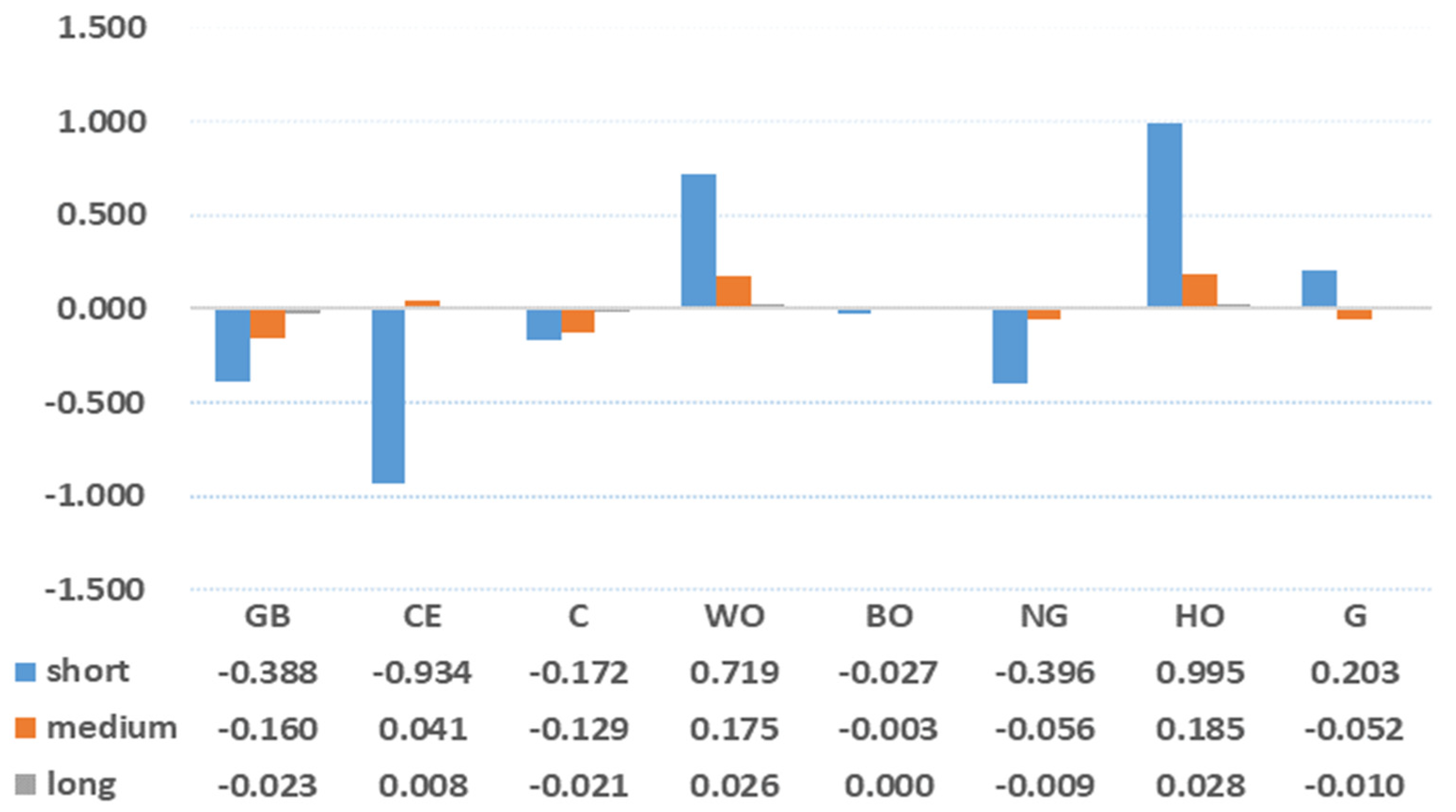
Figure 8 shows the net connectedness among the GB, CE, and fossil fuel markets in the short-, medium-, and long-term horizons. The net connectedness is variance transmission from another market to one market, which is a net giver/receiver of variance to/from all other markets if the net connectedness is positive/negative value. The volatility spillover of the other markets to GBs, coal, NG, and Brent is negative in all three sample terms (Figure 8), indicating their role as volatility receivers. In contrast, WTI and HO, having a positive value, are the sources of volatility spillover. Although the volatility spillover of CE to other markets has negative values in the short term (see blue rectangle in Figure 8), the value becomes positive in the medium- and long-term horizons; the opposite is true for the GB market.

6. Discussion

Our results suggested that using the Bayesian DCC-MGARCH model with the SMGED to estimate the correlations among the GB, CE, and fossil fuel markets yields optimal results, and that the correlation between them is time-varying because the values of a + b shown in Table 4 are less than 1.

The results further suggested that the GB market has a weakly negative correlation (0 to −0.2) with the CE stock market, which means that the CE stock market tends to rise when bond yields fall, and tend to slump when GB yields rise (Figure 5 (a: R2)). The effect may be attributed to the fact that there are no non-pecuniary motives associated with investors’ pro-environmental preferences for investing in CE stock and GBs. If such motives exist, investors may purchase CE stocks and GBs to drive their prices up, in which case their relationship becomes positive. Thus, these non-pecuniary motives may exacerbate the impact of CE stock price volatility on GBs, and vice versa.

In addition, our results suggest that the relation of fossil fuel to GBs and CE stocks has a negative or weak positive value (less than 0.4), which implies that GBs, CE stocks, and fossil fuels may be used as a portfolio to mitigate investment risk for energy investors because of the existence of a weak or negative correlation between them. When the relationship between one market and another market is negative or weakly correlated, the two assets can be mutual hedges for investment diversification based on the basis of the concept that an asset is a hedges asset if it is negatively correlated or uncorrelated with another asset (Baur and Lucey, 2010 [37]), and vice versa. We confirmed the result of Reboredo and Ugolini (2020) [3], who revealed that the linkage between GB, the energy index, and the stock index has a weak correlation, which is important for GB-holding investors to make risk portfolio decisions.

We also find that the volatility spillover among the GB, CE, and fossil fuel markets presents the strongest in the short term but gradually weakens from the medium term to the long term. Moreover, GBs are net volatility receivers from the WTI market and its related markets (HO and gasoline) in the long- and medium-term (Figure 8), indicating that investors holding GB assets should pay attention to the effects of WTI price volatility. This is because the crude oil market is susceptible to price volatility resulting from the effect of political and climatic factors (Lee et al., 2021 [23]); when the WTI price falls, investors might buy less risky GB to mitigate losses, thus facilitating the volatility spillover of WTI prices to the GB markets. This result implies that if GBs, CE, and crude oil are invested as a portfolio, the source of risk for the portfolio is mainly the volatility of WTI prices.

Finally, our results suggested that compared with Brent, WTI has a stronger relationship with GBs and CE (Figure 5b). Meanwhile, the volatility spillover of WTI to the GBs and CE markets is higher than that of Brent in the short-, medium-, and long-term horizons, while the volatility among them is higher in the short term, gradually decreases in the medium term, and disappears in the long term (Table 6, Table 7 and Table 8). A possible reason for this difference between WTI and Brent is that WTI is the U.S. crude oil price while Brent crude oil is a benchmark price for the European crude oil market (Aruga, 2015 [38]). Hence, the U.S. GB and CE prices are more likely to be connected to the WTI price. The result implies that in holding GBs and CE as a portfolio, investors need to pay more attention to the volatility spillover of WTI to manage risks. These results are somewhat different from those of Lee et al. (2021) [23], who indicated that the international Brent has a significant bi-directional causality from the global GB index.

In summary, the results of the relationship and volatility spillover among the GB, CE stock, and fossil fuel markets are consistent with those of Reboredo (2018) [2], Reboredo and Ugolini (2020) [3], Tiwari et al. (2021) [21], Dutta et al. (2021) [22], Lee et al. (2021) [23], and Pham (2021) [4], who suggested that the relation among them is time-varying and weakly positive or negative; these characteristics provide important information for managing portfolio risk. In addition, due to the occurrence of COVID-19, Rehman et al. (2023) [24] and Wang et al. (2022) [26] found that the impact of WTI oil on GB markets was positive in the short run, but these results do not consider how Brent oil affects GBs (not in US markets). Unlike the results of Rehman et al. (2023) [24] and Wang et al. (2022) [26], our study uses the Bayesian DCC-MGARCH model and frequency connectedness method to gain two results: first, the correlation and volatility of WTI and GBs are stronger than those of Brent oil and GBs because the WTI oil is independent relative to Brent oil in the US market; second, the correlation and volatility spillover of WTI to another market is different from those of Brent at different term horizons.

7. Conclusions and Policy Implications

In this study, the Bayesian DCC-MGARCH model is used to examine the correlation between GB, CE, and fossil fuel markets. Due to the AIC, BIC, and DIC information criteria values for SMGED being minimal, our study identifies that the Bayesian DCCM-GARCH model with the skew multivariate generalized error distribution is credible for GB, CE, and fossil fuel markets to estimate the time-varying conditional correlations between them. The frequency connectedness method is also applied to identify how the volatility spillover among them is transmitted and how it changes in the short-, medium-, and long-term horizons.

Our empirical findings can offer some valuable implications for investors and energy policymakers.

First, the GBs almost have a weakly negative correlation or zero correlation with fossil fuel and CE, suggesting that the GB market is independent of the CE and fossil fuel markets. This information helps investors realize the role of green bonds in diversifying against the fluctuation of fossil fuel markets, and encourages portfolio investors who want to achieve higher investment performance to include GBs in their portfolios. Moreover, for policymakers, this information also indicates that the GB market has limited influence on the CE and the fossil fuel markets.

Second, given that the GB and CE markets are net volatility receivers from WTI or its related energy markets (HO and gasoline) in the short term, the result is important for across-market investors to identify which market is the main risk receiver or transmitter and how the risk spillover of the fossil fuel market to the GBs and CE stock markets changes at different terms. Thus, policymakers should establish mechanisms (for example, to help deal with oil price risk, many governments have established oil stabilization funds) to stabilize the WTI market to reduce price volatility spillover risk, which is not only important for the investor to reduce losses, but develops the GB and CE markets for a sustainable economy.

Third, given that the correlation and volatility spillover of WTI to the GB and CE markets are stronger than those of Brent in the short term, gradually decrease in the medium term, and disappear in the long term, in developing the GB market, stakeholders should be aware that the spillover effect of WTI prices is different from that of Brent prices at different frequencies. Furthermore, policymakers should establish appropriate mechanisms for mitigating the effect of WTI on the GB market in the short and medium terms to ensure its issuance price stability. Such stability is important to mobilize financing for sustainable investment.

Thus, our conclusion resulting from our findings is that investors or policymakers should be aware that green bond investing addresses the two-pronged investment strategy of (i) risk diversification and (ii) carbon mitigation.

Our study has some limitations in that it demonstrates the internal validity of the results in the U.S. market. Hence, further research is needed to determine whether our results can be generalized to other countries to identify which market is the transmitter/receiver of volatility to manage risk in cross-market investment. In future research, we will consider the international GB market and other financial markets to test the external validity of our study.

References

- IEA. 2021. Available online: https://www.iea.org/data-and-statistics/data-product/world-energy-investment-2021-datafile#overview (accessed on 2 May 2021).
- Reboredo, J.C. Green bond and financial markets: Co-movement, diversification and price spillover effects. Energy Econ. 2018, 74, 38–50. [Google Scholar] [CrossRef]
- Reboredo, J.C.; Ugolini, A. Price connectedness between green bond and financial markets. Econ. Model. 2020, 88, 25–38. [Google Scholar] [CrossRef]
- Pham, L. Frequency connectedness and cross-quantile dependence between green bond and green equity markets. Energy Econ. 2021, 98, 105257. [Google Scholar] [CrossRef]
- Baruník, J.; Křehlík, T. Measuring the Frequency Dynamics of Financial Connectedness and Systemic Risk. J. Financial Econ. 2018, 16, 271–296. [Google Scholar] [CrossRef]
- Climate Bonds Initiative. 2020. Available online: https://www.climatebonds.net/resources/reports/sustainable-debt-global-state-market-2020 (accessed on 2 May 2021).
- Tang, C.; Aruga, K. Relationships among the Fossil Fuel and Financial Markets during the COVID-19 Pandemic: Evidence from Bayesian DCC-MGARCH Models. Sustainability 2022, 14, 51. [Google Scholar] [CrossRef]
- Ehlers, T.; Packer, F. Green bond finance and certification. BIS Q. Rev. 2017, 89–104. [Google Scholar]
- Banga, J. The green bond market: A potential source of climate finance for developing countries. J. Sustain. Finance Invest. 2018, 9, 17–32. [Google Scholar] [CrossRef]
- MacAskill, S.; Roca, E.; Liu, B.; Stewart, R.; Sahin, O. Is there a green premium in the green bond market? Systematic literature review revealing premium determinants. J. Clean. Prod. 2021, 280, 124491. [Google Scholar] [CrossRef]
- Pham, L. Is it risky to go green? A volatility analysis of the green bond market. J. Sustain. Finance Invest. 2016, 6, 263–291. [Google Scholar] [CrossRef]
- Zerbib, O.D. The Green Bond Premium; University of Chicago Press: Chicago, IL, USA, 2017; p. 52. [Google Scholar] [CrossRef]
- Zerbib, O.D. The effect of pro-environmental preferences on bond prices: Evidence from green bonds. J. Bank. Finance 2019, 98, 39–60. [Google Scholar] [CrossRef]
- Nanayakkara, M.; Colombage, S. Do investors in Green Bond market pay a premium? Global evidence. Appl. Econ. 2019, 51, 4425–4437. [Google Scholar] [CrossRef]
- Lebelle, M.; Lajili Jarjir, S.; Sassi, S. Corporate Green Bond Issuances: An International Evidence. J. Risk Financial Manag. 2020, 13, 25. [Google Scholar] [CrossRef] [Green Version]
- Pham, L.; Luu Duc Huynh, T. How does investor attention influence the green bond market? Financ. Res. Lett. 2020, 35, 101533. [Google Scholar] [CrossRef]
- Piñeiro-Chousa, J.; López-Cabarcos, M.Á.; Caby, J.; Šević, A. The influence of investor sentiment on the green bond market. Technol. Forecast. Soc. Chang. 2021, 162, 120351. [Google Scholar] [CrossRef]
- Tolliver, C.; Keeley, A.R.; Managi, S. Drivers of green bond market growth: The importance of Nationally Determined Contributions to the Paris Agreement and implications for sustainability. J. Clean. Prod. 2020, 244, 118643. [Google Scholar] [CrossRef]
- Tu, C.A.; Rasoulinezhad, E.; Sarker, T. Investigating solutions for the development of a green bond market: Evidence from analytic hierarchy process. Finance Res. Lett. 2020, 34, 101457. [Google Scholar] [CrossRef]
- Broadstock, D.C.; Cheng, L.T.W. Time-varying relation between black and green bond price benchmarks: Macroeconomic determinants for the first decade. Finance Res. Lett. 2019, 29, 17–22. [Google Scholar] [CrossRef]
- Tiwari, A.K.; Aikins Abakah, E.J.; Gabauer, D.; Dwumfour, R.A. Dynamic spillover effects among green bond, renewable energy stocks and carbon markets during COVID-19 pandemic: Implications for hedging and investments strategies. Glob. Financ. J. 2022, 51, 100692. [Google Scholar] [CrossRef]
- Dutta, A.; Bouri, E.; Noor, M.H. Climate bond, stock, gold, and oil markets: Dynamic correlations and hedging analyses during the COVID-19 outbreak. Resour. Policy 2021, 74, 102265. [Google Scholar] [CrossRef]
- Lee, C.-C.; Lee, C.-C.; Li, Y.-Y. Oil price shocks, geopolitical risks, and green bond market dynamics. N. Am. J. Econ. Financ. 2021, 55, 101309. [Google Scholar] [CrossRef]
- Rehman, M.U.; Raheem, I.D.; Zeitun, R.; Vo, X.V.; Ahmad, N. Do oil shocks affect the green bond market? Energy Econ. 2023, 117, 106429. [Google Scholar] [CrossRef]
- Su, C.W.; Chen, Y.; Hu, J.; Chang, T.; Umar, M. Can the greed bond market enter a new era under the fluctuation of oil price? Econ. Res. Ekon. Istraz. 2023, 36, 536–561. [Google Scholar]
- Wang, K.-H.; Su, C.-W.; Umar, M.; Peculea, A.D. Oil prices and the green bond market: Evidence from time-varying and quantile-varying aspects. Borsa Istanb. Rev. 2023, 23, 516–526. [Google Scholar] [CrossRef]
- Abakah, E.J.A.; Tiwari, A.K.; Adekoya, O.B.; Oteng-Abayie, E.F. An analysis of the time-varying causality and dynamic correlation between green bonds and US gas prices. Technol. Forecast. Soc. Chang. 2023, 186, 122134. [Google Scholar] [CrossRef]
- Fama, E.F. Effificient capital markets: II. J. Financ. 1991, 46, 1575–1617. [Google Scholar] [CrossRef]
- S&P Dow Jones Indices. 2021. Available online: https://www.spglobal.com/spdji/en/indices/esg/sp-us-municipal-GB-index/#overview (accessed on 1 November 2021).
- INSIDER. 2021. Available online: https://markets.businessinsider.com/ (accessed on 20 May 2021).
- Invesco. 2021. Available online: https://www.invesco.com/us/financial-products/etfs/product-detail?audienceType=Investor&ticker=PBW (accessed on 2 May 2021).
- Diebold, F.X.; Yilmaz, K. Better to give than to receive: Predictive directional measurement of volatility spillovers. Int. J. Forecast. 2012, 28, 57–66. [Google Scholar] [CrossRef] [Green Version]
- Shiferaw, Y.A. Time-varying correlation between agricultural commodity and energy price dynamics with Bayesian multivariate DCC-GARCH models. Physica A 2019, 526, 120807. [Google Scholar] [CrossRef]
- FIoruci, J.A.; Ehlers, R.S.; Louzada, F. BayesDccGarch—An Implementation of Multivariate GARCH DCC Models. arXiv 2014, arXiv:1412.2967. [Google Scholar]
- Mensi, W.; Vo, X.V.; Kang, S.H. Multiscale spillovers, connectedness, and portfolio management among precious and industrial metals, energy, agriculture, and livestock futures. Resour. Policy 2021, 74, 102375. [Google Scholar] [CrossRef]
- Maghyereh, A.I.; Abdoh, H.; Awartani, B. Connectedness and hedging between gold and Islamic securities: A new evidence from time-frequency domain approaches. Pacific-Basin Finance J. 2019, 54, 13–28. [Google Scholar] [CrossRef]
- Baur, D.; Lucey, B. Is Gold a Hedge or a Safe Haven? An Analysis of Stocks Bonds and Gold. Financ. Rev. 2010, 45, 217–229. [Google Scholar] [CrossRef]
- Aruga, K. Testing the international crude oil market integration with structural breaks. Econ. Bull. 2015, 35, 641–649. [Google Scholar]
Figure 1.
The investment size of the GB, fossil fuels, and renewable energy markets. Note: (a) is sourced from Climate Bonds Initiative, and (b) is sourced from IEA (2021) [1].
Figure 2.
The related variables studied between 3 January 2019 and 26 February 2021. (a) The logarithmic prices among green bond, clean energy, WTI oil, and Brent oil; (b) The logarithmic prices of another fossil fuels.
Figure 3.
The fossil fuel, clean energy, and green bond price return series. Source: own calculation. (a) The prices return among green bond, clean energy, WTI oil, and Brent oil; (b) The prices return of another fossil fuels.
Figure 4.
Heat map of the correlation.
Figure 5.
The dynamic conditional correlation between GB, CE, and fossil fuel price returns. (a) The correlation of WTI oil and Brent oil, green bonds and clean energy; (b) The correlation of clean energy and green bonds with oil; (c) The correlation between green bond and another fossil fuels; (d) The correlation between clean energy and another fossil fuels; (e) The correlation between WTI oil and another fossil fuels; (f) The correlation between Brent oil and another fossil fuels.
Figure 6.
The volatility spillover among interesting markets. Notes: d1: {2–4} days; d2: {4–8} days; d3: {8–16} days; d4: {16–32} days; d5: {32–64} days; d6: {64–128} days; d7: {128–256} days; d8: {256–512} days; WTI oil: WO; Brent oil: BO; gasoline: G; coal: C; natural gas: NG; clean energy: CE; green bond: GB; heating oil: HO. (a) Volatility spillover of another market to GB; (b) Volatility spillover of another market to CE; (c) Volatility spillover of another market to Brent; (d) Volatility spillover of another market to WTI; (e) Volatility spillover of another market to C; (f) Volatility spillover of another market to NG; (g) Volatility spillover of another market to HO; (h) Volatility spillover of another market to G.
Figure 7.
The net pairwise directional connectedness of shock on different frequency bands. Notes: coal: C; gasoline: G; WTI oil: WO; Brent oil: BO; heating oil: HO; clean energy: CE; green bond: GB; natural gas: NG. (a): Short−term; (b): Medium−term; (c): Long−term.
Figure 8.
The net risk spillover of shock on short-term, medium-term, and long-term horizons. Notes: The same as the notes in Figure 7.