
Improving Functional Connectivity in Developmental Dyslexia through Combined Neurofeedback and Visual Training


Institute of Neurobiology, Department of Sensory Neurobiology, Bulgarian Academy of Sciences, Acad. G. Bonchev Str. bl. 23, 1113 Sofia, Bulgaria
*
Author to whom correspondence should be addressed.
Symmetry 2022, 14(2), 369; https://0-doi-org.brum.beds.ac.uk/10.3390/sym14020369
Submission received: 1 December 2021
/
Revised: 28 January 2022
/
Accepted: 10 February 2022
/
Published: 13 February 2022
(This article belongs to the Special Issue Simulation and Modelling in Natural Sciences, Economics, Biomedicine and Engineering II)
Abstract
:This study examined the effects of combined neurofeedback (NF) and visual training (VT) on children with developmental dyslexia (DD). Although NF is the first noninvasive approach to support neurological disorders, the mechanisms of its effects on the brain functional connectivity are still unclear. A key question is whether the functional connectivities of the EEG frequency networks change after the combined NF–VT training of DD children (postD). NF sessions of voluntary α/θ rhythm control were applied in a low-spatial-frequency (LSF) illusion contrast discrimination, which provides feedback with visual cues to improve the brain signals and cognitive abilities in DD children. The measures of connectivity, which are defined by small-world propensity, were sensitive to the properties of the brain electrical oscillations in the quantitative EEG-NF training. In the high-contrast LSF illusion, the z-NF reduced the α/θ scores in the frontal areas, and in the right ventral temporal, occipital–temporal, and middle occipital areas in the postD (vs. the preD) because of their suppression in the local hub θ-network and the altered global characteristics of the functional θ-frequency network. In the low-contrast condition, the z-NF stimulated increases in the α/θ scores, which induced hubs in the left-side α-frequency network of the postD, and changes in the global characteristics of the functional α-frequency network. Because of the anterior, superior, and middle temporal deficits affecting the ventral and occipital–temporal pathways, the z-NF–VT compensated for the more ventral brain regions, mainly in the left hemispheres of the postD group in the low-contrast LSF illusion. Compared to pretraining, the NF–VT increased the segregation of the α, β (low-contrast), and θ networks (high-contrast), as well as the γ2-network integration (both contrasts) after the termination of the training of the children with developmental dyslexia. The remediation compensated more for the dorsal (prefrontal, premotor, occipital–parietal connectivities) dysfunction of the θ network in the developmental dyslexia in the high-contrast LSF illusion. Our findings provide neurobehavioral evidence for the exquisite brain functional plasticity and direct effect of NF–VT on cognitive disabilities in DD children.
1. Introduction
Neurofeedback (NF) has received increasing amounts of attention in the treatment of various neuropsychological and cognitive disorders. NF stimulates the important characteristics of the neural activity; converts them into visual, auditory, or tactile feedback; rewards desired patterns; and inhibits unwanted patterns in the brain activity in order to trigger a training process. The NF training can increase the plasticity of the brain through a learning process with reinforcement [1]. NF-induced plasticity can compensate for neurological deficits [2,3] and cognitive disabilities [4]. The NF efficiency depends on many factors in the spatial, frequency, and temporal domains. The spatially localized brain area that generates the NF signal is targeted to specific functions. The NF goals in the frequency domain can be achieved through specially selected electroencephalographic (EEG) rhythms. The z-score neurofeedback implements a quantitative online EEG technique (qEEG z-NF) for the training of the brain activity with EEG metrics (power, amplitude, coherence, and phase), generates the z-scores from many brain areas to normative data or to the reference values of healthy people [5,6], and converts the z-scores into feedback signals [7,8].
The training to discriminate visual patterns depends on the latency of the feedback signal [9]. The type of training, which can be network training or behavioral training, directs the training’s effect onto the brain’s ability to improve its cognitive performance [10]. The network training involves the practice of a specific task (e.g., attention, working memory) with a fixed difficulty, or adaptive training with an adjusted task difficulty, and it exercises the specific task-related brain areas and networks until the performance over the course of the trials is improved [11]. Increased task-related brain activity may reflect greater efforts to discriminate more complex tasks during adaptive training [12], while the enhanced neuronal adaptation during the experiment may reduce the cognitive demands for the activation of the stimulus-related brain regions.
EEG-NF training has shown improvements in the cognitive-behavioral indices and diminished EEG abnormalities of learning-disabled children (LD) [13,14,15]. Altered brain functions in dyslexia show a left-lateralized hypoactivation of the posterior brain systems in the ventral occipitotemporal and temporoparietal regions, which are part of the brain’s network in typical readers, and are adapted to reading in dyslexia [13,14,15]. High θ and low α activity in LD children suggests a maturation lag in the cognitive neural networks [16,17].
The qEEG z-NF efficacies in children and adolescents with LDs after 10 sessions correlated with improvements in the academic and behavioral problems reported by their parents [6]. The NF θ-to-β protocol might be efficient at compensating for attentional deficits [18,19,20,21,22]. The z-scores within a defined range stimulated the brain to establish its own route towards self-regulation [8], and to achieve the most relevant goal-directed behavior. Poorer cognitive performances in children and adolescents with LDs are associated with a neural network deviation from normal development, which manifests as an α-frequency EEG maturation delay [16,17,23]. The α-waves acquire their highest amplitudes [5,24,25] mainly in the posterior brain regions, and are highly stable in time and are sensitive to the developmental changes in cognitive neural networks [26,27,28]. The α-waves are generated by thalamocortical feedback loops and they reflect the information-processing speed, which are important processes for the working and semantic memories [26,27,28]. The children with LDs and attention-deficit/hyperactivity disorders (ADHD) show low α-bands (<9 Hz) compared to age-matched typically developed children [17,24,29,30]. The slow α-peak frequency (<9 Hz) in LD children is considered to be a biomarker [30]. These children are classified on the basis of the categories of the amplitude peak frequencies and their responses at the qEEG z-NF intervention, with multiple abnormal z-scores of the excess focal δ or θ, atypical α, fast frequencies in multiple regions, and increased generalized delays and asymmetries [16,29].
The α/δ NF [31], the θ/α z-NF [29], and the θ/α training protocols [32] specify only two bands. The associated clinical symptoms and improvements are due to the NF training of the regions involved in a specific task. The δ-frequency band (<4 Hz) was chosen as the frequency for inhibition in the α/δ protocol, and the training-induced changes were mainly related to increases in the α-frequency range. The over-recruitment in the low-frequency bands (δ, θ) is associated with sustained concentration and attention, while the under-recruitment in the high-frequency bands (γ, β) at the parietal and temporal cortices is associated with response preparation and memory maintenance [33]. Low α (8–13 Hz) and high β (15–30 Hz) spectral powers, particularly during the prestimulus period, characterize the increased attention and predict better ongoing task performances [34,35]. The increased prestimulus right-hemispheric β-band power may reflect the attentional network activation [36,37], or the activation in a region engaged in the ongoing stimulus processing [38]. The increased prestimulus θ and the α-band power may indicate the fatigue accompanying the experiment [39].
The NF training reinforces the θ/α reduction and treats learning disorders [32]. The most reported EEG patterns for reading-disabled children (RD) have redundancies of slow θ-frequency activity [40,41], α-activity deficit [42], and delayed EEG maturation [40], compared to typically developed children. Most EEG studies of the brain activity in LD children are based on EEG power analyses; however, few have focused on the measure of functional connectivity as coherence [32]. The coherence neurofeedback [43] on the participants with dyslexia show the hypocoherence of the occipitoparietal lobes to the frontal-temporal lobes, and a hypocoherence of the parietal to the medial–temporal connections. Hypocoherences have been reported on the δ-, θ-, and α-frequency bands. Coherence is the measure applied in the clinical setting between the EEG sensors. Higher δ and θ-frequency coherence, and lower α-frequency coherence are typical EEG characteristics for RD children [44], when compared to normal readers. The interhemispheric δ-, θ-, and β-frequency coherences diminish mainly between the frontal regions, as well as the intra-hemispheric δ, θ, and β coherences, while they increase in the α-frequency band. The reduced θ-frequency coherence in the left hemisphere between the frontal and other regions is particularly important for reading. This lower α-frequency coherence is replicated in adults with dyslexia [45]. In general, there is a tendency for increased frequency coherence in development, except for the θ-frequency band [46]. Lower interhemispheric coherences and higher intrahemispheric coherences characterized the children with dyslexia, compared to their peers [47]. The NF θ/β training protocol was effective for Chinese children with dyslexia [48]. Reducing the θ-frequency coherences in the inferior frontal and middle temporal regions, which are adjacent to the Broca area, enhanced the spelling abilities but not the reading [49]. The coherent protocols for people with dyslexia improved the reading and the phonological awareness [43,50]. People with dyslexia also have slow waves at Broca’s area and no desynchronized β1 activity in Broca’s area and in the angular gyrus during reading tasks [51], nor in the left occipitotemporal and occipital regions [52]. Dyslexic children have increased slow activity in the right posterior superior temporal, occipitotemporal, and parietal regions, and in the frontal lobes [53]. There is a symmetric hypercoherence for the δ- and θ-frequency bands at the bihemispheric posterior superior temporal lobe, and a specific right-temporal hypercoherence for the α- and β-frequency bands [53]. Hypercoherence in the bihemispheric middle temporal lobes manifests in the δ- and θ-frequency bands, while hypocoherence can be found between the left occipitotemporal and occipital regions in the δ-, θ-, and α-frequency bands [43], which means that left-hemispheric dominance is not yet established. Therefore, any training of dyslexia should improve the left hemispheric functioning. Although one study combined qEEG neurofeedback sessions and multisensory learning methods for reading in children with developmental dyslexia (DD) [54], there are no qEEG NF protocols that collaborate with training tasks for the various visual deficits in children with DD, which could provide a more effective way to improve their learning abilities. Slow-wave neurofeedback reduced them to the stage where the brain is ready to learn new information, and the neural system should then seamlessly connect the visual representations of the lexemes with the phonemes. This process is repeated many times, as there are differences in the cross-modal processing to make it in a permanent ability in dyslexia [54,55]. The training computer tasks efficiently repeat the same procedure to stimulate the appropriate neural mechanisms in the DD children. Multisensory training for DD children [54,55] does not change the brain structure but it does improve the perceptual processes. Another study of dyslexic children used NF game-based cognitive training and reported that both intelligence and attention improved [56].
In the current study, we explore the qEEG z-NF α/θ protocol to reinforce the θ inhibition, the α activity, and the effective EEG reorganization, and to enhance the cognitive-behavioral performance. The qEEG z-NF protocol in children with developmental dyslexia was combined with training for the various visual deficits in dyslexia, and it could positively affect the functional connectivity of a specific frequency network that is also involved in the reading process. The selective inhibition of the excitatory neurons in a brain hub (region) can change the network integration [57]. Reduced network integration can result from the selective suppression of the excitatory neurons in a hub. The dysfunction of the brain hub can affect the segregation, the resilience, and the network topology, which can lead to large-scale changes in the brain network. The hypotheses are: (1) The suppression of a hub can affect widespread brain hub–node connections and the entire network organization; (2) Through reductions in the hub centrality and strength, its role as a hub can be lost; and (3) A new hub can appear through an increase in the centrality of the node after the hub suppression, or after the deactivation of an existing hub. Our study aimed to modify the global brain functional connectivities and the efficiencies of the reading circuits in children with developmental dyslexia, as well as those of normally reading children, through 12-channel qEEG z-NF interventions on specific brain locations (hubs) in children with dyslexia, which was combined with visual training tasks.
On the basis of the functional connectivities of the typically developed children, we suggest that qEEG z-NF could produce a functional reorganization in DD children that consists of reduced intrahemispheric low-frequency δ or θ bands, and increased α in the regions involved in the reading network in the left hemisphere in the posterior part of the superior temporal lobe (classically referred to as Wernicke’s area), which is specialized in the phonological functions, and in the ventral occipitotemporal cortex, adjacent to the visual-word-form area, which is specialized in visual and orthographic recognition on the basis of memory, and in the inferior frontal cortex (classically called Broca’s area), which intervenes in the articulation and gesticulation of words [58,59,60].
2. Materials and Methods
2.1. Participants
The data for the group with developmental dyslexia (DD children, n = 72; 52 boys and 20 girls) and the control group (n = 36; 26 boys and 10 girls; mean age: 8–9 years; SD = 0.58) were analyzed after the exclusion of records with missing data. The study did not include children with disabilities unrelated to reading, as diagnosed by ophthalmologists and neuropediatricians [61,62]. The specific DD profile of the experimental group, along with the baseline control descriptive data, has been shown in previous works (Table A1; [60]). The inclusion criteria for the dyslexic children were as follows: (1) Diagnosed with DD by school logopedics and psychologists, according to the classification of DD children [63,64,65,66]; (2) Aged between 8 and 9 years; (3) With qEEG patterns of several abnormal waves in several brain regions; (4) Having completed 12 qEEG z-NF sessions targeting the Fz, Cz, Oz, FT9-10, TP7-8, Pz, PO7-O8, and O1–O2 locations; (5) Completion of visual training; and (6) An average intelligence quotient, which was estimated according to the Raven intelligence scale [67].
The study is a controlled trial comparing the interventions of the group with DD to a control group. The children with dyslexia were assigned to a pretraining group (preD), where they received six qEEG z-NF intervention sessions in a one-week period. These pretest sessions were administered in order to identify those with main (magnocellular) visual deficits, which further supports the notion of the multisensory integration deficit underlying dyslexia. To be effective, remedial intervention should not be fuzzy, and should focus on the deficient skills. Therefore, for the period of four months, the second-grade DD children underwent an intervention with a visual-based training procedure and six other qEEG z-NF sessions (treatment group or post-training group (postD)). The control group in the study contained normal age-matched readers (same school grade and sociodemographic background, no dyslexia, and no learning or language disabilities) who did not receive the intervention. The behavioral measures of reading were measured at the start and at the end of the four-month period (intervention) for both accuracy and speed, which included word reading as an assessment of the training benefits. The EEG functional measurements of the visual task were measured at baseline and at the end of the intervention (after four months) for the intervention group, and they were measured once for the control group (used as a criterion point to compare the pre/post EEG changes in the intervention). The study used a pretest–training–post-test design to evaluate the training effect of the combined programs (12 completed qEEG z-NF sessions and visual training) on the basis of the visual tasks, with a specific focus on the gains in the brain functioning related to reading skills. In the pretest–training–post-test design of the study, the group with dyslexia received an average of 366 sessions. The criteria for the intervention study were focused on specifying the underlying mechanisms of change for a sufficiently large sample in order to reduce the possibility that the results of the intervention occurred by chance. On the basis of the data of previous intervention studies [68], which show that a sample size of higher than 20 per intervention condition and an anticipated attrition rate of 20% achieved a good intervention effect, we recruited 72 children with dyslexia to detect the intervention effect on the significant remediation of their reading skills. Because of the proven stability in the reading abilities of the second-grade controls [68], we recruited a small size of the control group, which was limited to 36. The time between the measurements did not change the standardized scores of the second-grade controls [68], and, therefore, the controls had no post-test control measurements, and they did not undergo the visual training protocol.
2.2. Experimental Paradigm
The successful ways to promote DD children include engaging their attention with the use of reinforcement techniques (NF), and using visual stimuli with different orientations, spatial frequencies, locations, contrasts, and directions, as well as tasks with attention requirements [69].
Our reinforcement technique (neurofeedback) maximally activated the magnocellular pathways in the children with developmental dyslexia [70,71]. The task included the contrast discrimination of the illusionary doubling motion of a sinusoidal grating with a low spatial frequency (LSF) (2fd: two cycles per degree (cpd) of the visual angle; vertical flicking with 15-Hz counter phase), embedded in an external noise field. The LSF illusion task (Figure 1) comprised two conditions (low- and high-contrast grating), presented in 40 trials (with 20 trials per condition), in a pseudorandomized sequence, with an interstimulus interval (ISI) of 1.5–3.5 s. The contrast levels were 6% and 12% of the thresholds selected in the previously performed psychophysical contrast-sensitive tasks [72]. Each trial started with a fixation white cross for 100 ms. After 200 ms, a flicking sinusoidal grating appeared in the center of the screen for 200 ms, and with a viewing distance of 210 cm. Gabor’s oscillating grating is perceived at twice the spatial frequency of the actual spatial frequency.
A subsequent fixation period of 100 ms of a color cross was presented on the screen, which changed to red/green when the selected EEG activity was below/above the set threshold, respectively. The child discriminated the low-contrast sinusoidal grating by pressing a button with the left hand, and discriminated the high-contrast sinusoidal grating by pressing a button with the right hand. A brief beep marked the trial’s end. A response-time period from 100 to 1500 ms began with the stimulus onset. The reaction times less than 0.100 s and more than 1.5 s were excluded as outliers. The correct answers and the reaction times were taken into account. The refresh rate of the computer screen was 60 Hz, with a pixel resolution of 1920 × 1080. The stimuli were generated with in-house software written on C++ [72], and they were synchronized with the EEG data acquisition system. The children received trial-by-trial neurofeedback in the form of different colored crosses.
2.3. EEG Signal Preprocessing
The EEG experimental procedure has been described elsewhere [59]. The EEG sensors (Brain Rhythm Inc., Taiwan) were placed according to a 10–20 system [73,74], which covered: the middle frontal gyrus (MFG) (Fz, F3-4: Brodmann area, BA8); the postcentral gyrus (PSTCG; C3-4: BA123/6, primary somatosensory and motor cortices); the posterior part of the superior temporal gyrus (STG) (T7-8: BA21/22, [74]; MT/MST; [75]); the inferior parietal lobe (IPL) (P3: BA39/7/19—angular/precuneus/associative visual V3 areas; P4: BA39/40/7—angular/supramarginal gyri/precuneus; PGp/PGa/IPS/7P [76]; LIP [75]); the middle occipital gyrus (MOG) (O1-O2: BA19—associative visual V3 area); the precentral gyrus (PRECG) (Cz: Brodmann areas, BA4/6—primary motor, premotor cortices); the superior parietal gyrus (SPL) (Pz: BA7, precuneus, 7P; [76]); and a part of the cuneus of the occipital lobe (Oz: BA18—cuneus, visual area V2). Additional EEG sensors were arranged in the 10–10 system [73,74], which covered the adjacent brain areas to: the superior frontal cortex (SFC) (AF3-4: BA9—dorsolateral prefrontal cortex (DLFC)); the inferior frontal gyrus (IFG) (F7-8: BA45/47—Broca’s area, orbital frontal cortex); the anterior part of the inferior temporal gyrus (ATG) (FT9-10: BA20/BA38—temporal pole; TE/AIT areas; [76]); the middle frontal gyrus (MFG) (FC3-4: BA6—premotor and supplementary motor cortices: pre-SMA, SMA); the inferior frontal gyrus (IFG) (FC5-FC6: BA44/45—opercular and triangular parts of Broca’s area); the PRECG (C1-2: Brodmann areas, BA4/6/123—primary motor, premotor, somatosensory cortices); the PSTCG (C5-6: BA123/40/43—primary somatosensory cortex and supramarginal gyrus with extension into the Sylvian fissure to PFop; [75]); the SPL (CP1-2: BA5/7—PGa/7A/7PC; LIP areas; [76]); the IPL (CP3-4: BA40/123—supramarginal gyrus (subareas PFt/PFm; [76]); the ventral intraparietal sulcus VIP or IPSmot; [75]); the middle temporal gyri (MTG) (TP7: BA21/37/22—MT+/V5/MST; TP8: BA21/22/37/20—medial superior and middle temporal areas, lateral occipitotemporal/posterior inferior temporal gyri, adjacent to posterior fusiform/lingual gyrus; MST/MT+/V5/V4; [76]); the ITG (P7: BA37/19—lateral occipitotemporal gyrus, adjacent to posterior fusiform/lingual cortex, V5/V3; [76]); P8: BA37—occipitotemporal gyrus); the superior occipital gyrus (SOG) (PO3: BA19/18/39/7—dorsal visual cortex/parieto–occipital sulcus/angular gyrus/precuneus; pIPS/V3A/POs; PO4: BA19/18/39—dorsomedial parieto-occipital visual V6 and V6A, ventral portion of posterior intraparietal sulcus, including dorsal portion of retinotopical V3A/V7; [76]); and the MOG (PO7-PO8: BA18/19—ventral visual cortices V3v/V2). The ground sensor was placed on the forehead, and the reference sensors were placed on both mastoid processes. The skin impedance was less than 5 kΩ.
The continuous EEG data, with a sampling rate of 250 Hz, was band-pass filtered from the δ to the γ frequencies (δ = 1.5−4; θ = 4.5−8; α = 8.5−13; β1 = 13.5−20; β2 = 20.5−30; γ1 = 30.5−48; γ2 = 52−70 Hz). The artifact-free trials (not exceeding ± 200 µV), which were time-locked to the stimulus onset, were segmented for the functional connectivity analysis with a duration of 800 ms. After that, the remaining trials were filtered (bandpass: 1–70 Hz; notch filter: 50 Hz). The analysis included only the trials with correct responses to the corresponding contrast discrimination of the LSF illusion, within a time window of 0.1–1.5 s. After the preprocessing, the average trial number per condition and group was 772 artifact-free data epochs.
2.4. Neurofeedback Online Training Measures
The main question in our study was whether closed-loop neurofeedback through the EEG signatures of the target-induced oscillations can compensate for the magnocellular deficit in dyslexia and enhance the child’s performance in a visual illusion task.
The 12-channel online z-score neurofeedback device (qEEG z-NF) (sensors: Fz, Cz, Oz, FT9-10, TP7-8, Pz, PO7-PO8, O1-2) provided a 24-bit conversion with an internal sampling rate of 1024 samples/s and a 256-samples/s data rate to the computer. Each qEEG z-NF trial was online decoded in the frequency bands: δ (4 Hz); θ (4.5–8 Hz); α (8.5–12 Hz); β1 (13.5–20); β2 (20.5–30 Hz); and γ (30.5∓48; 52∓70 Hz), by a Morlet wavelet during the time of the sinusoidal grating presentation (~250 ms; MATLAB function). The individual amplitude peaks of the α and θ frequencies defined the qEEG z-NF α/θ scores for eight brain regions in each hemisphere. The software contained normalized data defined by the prefeedback baseline mean measure, which was taken during a 2.5-min feedback-free period with eyes opened at the beginning of the first session of children, and which was used to determine the z-NF α/θ scores’ thresholds. The absolute pre-z-scores ≥ 1.0 were highlighted as being the targeted z scores by site and frequency [7]. The enrolled potential candidates for the feedback were based on multiple abnormal qEEG z-NF α/θ scores from several of the brain locations studied in dyslexia [59,60]. The time interval from the neural activity to the delivery of the qEEG z-NF to the child (NF latency) was set to significantly affect the outcome of the operant conditioning that specified the reinforcement schedule [77]. The qEEG z-NF α/θ score was delivered via the sensor with the highest z-value back to the child as a color cross on the screen. This reinforcement was based on the z-score that falls above the threshold (positive z-score rewards visual feedback with green cross) and under the threshold (negative z-score rewards visual feedback with a red cross). A neurofeedback α/θ protocol was applied to the dyslexic group in six sessions of 10 min for the left brain hemisphere, and 10 min for the right brain hemisphere.
The qEEG z-NF α/θ protocol was as follows: (1) Intrahemispheric reduced θ and increased α waves in the left hemispheric regions in the reading functional network, which is adjacent to the posterior superior temporal (Wernicke’s area) and middle occipital gyri, and the ventral occipitotemporal cortex, which is adjacent to the visual-word-form area, and the left inferior frontal cortex (Broca’ area); and (2) Increased the left hemispheric qEEG z-NF α/θ scores and reduced the right hemispheric qEEG z-NF α/θ scores, which compensated for the brain laterality. By applying neurofeedback, the slow brain waves should be reduced to a level where the brain is prepared to learn new information.
This qEEG z-NF α/θ protocol was administered twice for the dyslexic group and once for the control group, and it included the qEEG z-NF treatment (six sessions) before the visual training procedure, and then four months after that, in the next six qEEG z-NF sessions. The mean number of qEEG z-NF sessions from the preassessment to the postassessment for the dyslexics was 12. The qEEG z-NF sessions in the first experiment period were separated from the visual perceptional training.
2.5. Visual Training Procedure
The visual training procedure [78] was directed towards a wide range of visual functions (i.e., the spatial attention with the accurate gaze direction, the enhanced contrast sensitivity in fine or coarse conditions, the processing speed, and the direction discrimination of the coherent motion in crowded paradigms with eye movement training). The visual training (VT) consisted of discrimination tasks in which the stimuli unpredictably appeared in the center of a screen. The children had to direct their attention and gaze to the stimulus (or the stimuli). These task-mediated improvements are believed to target multiple features, which heighten the changes for the broader modal transfer [79]. The learning effects in them are negligible, according to the reported effects of the training [55,69,72].
The procedure was the same for all of the participants with DD [55,78]. The children underwent baseline measurements with five visual and two auditory tasks, and then the dyslexics were trained with six qEEG z-NT sessions. After that, only the dyslexics performed VT [55], which consisted of five visual tasks with two blocks (conditions), with 40 trials, three times per week, for approximately 12 consecutive weeks, which makes a total of 11,600 trials per child. The children relaxed between the tasks.
All of the dyslexic children trained at school with visual training tasks [55,72]. Before the subjects started the training, they received verbal instructions about the computer tasks, monitoring of the actual viewing distance for each task, and information on how to respond with buttons on the task controller. At the end of each training task, the task sent the data to a monitor, which allowed for the monitoring of the training compliance.
The training program, which was based on the low-contrast discrimination of the low-spatial-frequency sinusoidal gratings (2 cpd), and high-temporal frequencies (15 reversals/s), which were vertically flicking in the external noise region, had the same experimental parameters and requirements as the abovementioned reinforcement technique.
The next training program, which was based on the high-contrast discrimination of high-spatial-frequency sinusoidal gratings (10 cpd), which were vertically flicking in the external noise region, with contrast levels of 3 and 6% of the defined contrast thresholds in previous psychophysics paradigm [55], was used to increase the parvocellular pathway. The other parameters of the task and the children’s requirements were the same as in the previous training task.
The training program, which required the direction discrimination of the coherent vertical motion [55], stimulated the magnocellular function. The coherent vertical motions of the white dots in randomly moving elements, with a size of 0.1 deg within a circle (a diameter of 20 deg), appeared on a black screen, at a viewing distance of 57 cm, for 200 ms. The velocity of the moving dots was 4.4 deg/s. The coherent motion threshold was 50% of the randomly moving dots. The ITI was 1.5–2.5 s. The instructions were the press of a button with the left hand for an upward motion of the dots, and the press of a different button with the right hand when the dots moved downwards.
The velocity discrimination training program induced changes in the MT/V5 brain area [55]. Two pairs of circular stimuli, with the radial moving the white dots’ elements from the center to the periphery of the optical flow (a diameter of 10 deg), appeared sequentially, one after another, on a screen. Each stimulus pair’s first item was always performed with a constant slow speed (4.5 deg/s). The second item in the pair of stimuli had the speed of the flow (5.0 deg/s) close to that of the first stimulus (4.5 deg/s), or with a higher speed (5.5 deg/s). The first item appeared for 300 ms, and after 500 ms, the second item in the stimulus pair appeared for 300 ms at a viewing distance of 57 cm. The ITI was 1.5–3.5 s. The instruction was to press a key with the right hand when the pair’s speed was slow, or press another key with the left hand when the second stimulus in the pair had a higher speed than the first stimulus’s constant speed.
The aim of the visual-spatial attentional training task was to search and track either the color change or the color preservation of a square in a cue [55]. The cue was a black frame for 300 ms, in either the left or right visual fields on a white screen, before the square color array (each with a size of 3 × 3 deg) presentation. A color square appears in the cue for 200 ms, horizontally or vertically, in an arranged color array of four squares. The cue remains on the screen during the presentation of the color array. The child had to compare the square color in the cue with the previous one presented in it on the screen at a viewing distance of 57 cm. The adjacent squares in the array changed their colors in every presentation. The ITI was 1.5–2.5 s. The child pressed a key on a computer keyboard with the left hand when two consecutive colors in the cue were the same, and with the right hand when they were different. The number of correct answers and the reaction times were reported in the training programs, with 40 trials for each condition and task. The thresholds of the parameters and the program designs have been described in previous works [55].
Four months later, the second set of qEEG z-NF post-training measurements was taken to determine the long-term training effect. The training sessions were opened for the children after each task, and they provided them with information on a screen about the percentage of successful trials for each task and condition. The children and their parents also received written informed consent, including the General Data Protection Regulation rules (EC/2018; BG Personal Data Protection Law/LPPD-26.02.2019), and a training protocol with instructions concerning the desired training tasks, which were approved by the Ethics Committees of the Institute of Neurobiology and the Institute for Population and Human Studies, BAS (approval No 02-41/12.07.2019), the State Logopedic Center, and the Ministry of Education and Science (approval No 09-69/14.03.2017).
The metrics of the functional connectivities were calculated before and after the training (qEEG z-NF and VT). We analyzed the pre- and post-training differences for the behavioral performances and the functional connectivity measures during the illusion task.
2.6. Small-World Propensity
The phase lag index (PLI) defines the phase synchronization across all sensor pairs [79,80], which are not phase-locked when the PLI is 0, and with a phase difference between the pairs different from 0 mod π when the PLI is 1 [80,81]. The PLI is less sensitive to spurious correlations because of the co-sources in the brain and its volume conduction. The statistical calculations over the strengths of the node connections form the networks. Metrics such as hubness, integration, and segregation reflect the network behavior on a global level [82,83]. The network’s ability to process specific information locally within the adjacent brain areas is its network segregation, while its integration is the ability to combine information from different brain regions (nodes) [84]. The fractions of the nodes’ neighbors, which are neighbors of each other, define the clustering coefficient, which characterizes the brain network segregation [85,86]. The shortest path length averaged between all the nodes’ pairs characterizes the network integration or, i.e., the so-called “characteristic path length” [85,86]. The measures for the hubness are the connection strength of a node compared to the other nodes, and the betweenness centrality of a node (fraction of the shortest paths passing through a node) [82,83,87]. The fraction of the shortest paths containing a given link is the betweenness centrality (BC) of the edges. The inverse of the average path length quantifies the exchange of information across the entire network and quantifies the network efficiency. The ratio of the clustering coefficient, the characteristic path length, and the global efficiency define the small world of the network [83]. A new graph metric, namely, small-world propensity (SWP), assesses the small-world network structures with different densities, while considering the variations in the network density [88] and the sensitivity to the functional connection’s strengths between the nodes. The contributions of the weak and strong links are differential to the overall network functioning [89]. This method does not apply threshold techniques to remove the weak links, as does other approaches, because these links can be potential pathological biomarkers [89].
The SWP defines the properties of the small worlds of the weighted networks (ϕ), as compared to the metrics (clustering coefficient, characteristic path length) of the regular lattices and random graphs with the same node numbers and the same degrees of the probability power distribution of the overall nodes in the real network [88]. The deviation of the clustering coefficient (∆C of Cobs) and the characteristic path length (∆L) of the observed network (Lobs) from its null model as a random network and regular lattice quantifies the SWP (ϕ) of the observed network. The assumptions in these models are that the closer nodes in the network have stronger node–node connection strengths and stronger edges than the distant network nodes. The ϕ of the observed network is evaluated by these reference networks. The characteristic path length value is low, and the clustering coefficient is high for the lattice network, while the characteristic path length is high, and the clustering coefficient values are low for the random network. At a maximal deviation of the clustering coefficient from its null model, the network rewires. The randomly distributed weighted edges between the N nodes create the random network, with small shortest paths and randomly assigned connections throughout the matrix. The random network model is not segregated and is highly integrated when there is no significant local clustering between the nodes. The path lengths, or the clustering coefficients, of the real networks can exceed the lengths of the random or lattice networks. The ϕ sets to 1 when the weighted networks’ measures are more than 1, and it sets to 0 if the weighted networks’ measures are less than 0. The ϕ is close to 1 when the observed network has high clustering and low path lengths, which equally contribute to the ϕ (i.e., low deviations of the ΔC and ΔL). The brain networks with large ϕ values exhibit small-world properties. Larger deviations of the measures (path length and clustering) of the observed networks from those of their null models define the lower ϕ values of the networks with less small-world structure [88]. The relatively high ϕ leads to modest clustering and a short path length (moderate ΔC and low ΔL, respectively), as well as to a moderate path length and high clustering (moderate ΔL and low ΔC, respectively). The real power of the ϕ quantifies the degree of the small-world graph between the different networks.
The weighted adjacency matrices (40 × 40), which are constructed by the PLI between all the pair channels, are estimated in the δ- to γ-frequency bands. The ϕ, ΔL, and ΔC are defined for the controls and dyslexics by the MATLAB toolbox for brain connectivity [88].
The weights of the adjacency matrix are converted into distances and they determine the betweenness centralities (BCs) of the nodes. A large number of the shortest paths involve edges with high values of the betweenness centrality. The sum of all the connection weights for a node determines the node strength (the BC values), which is divided by the average local measures of all the nodes. Nodes with strength (high BC) play a significant role in the processing of information in the graph and they are involved in the many shortest paths [86]. Graphs are more integrated when there is a higher maximum BC, or strength [82,87]. The most important nodes of the network are the hubs, which were obtained through MATLAB’s brain connectivity toolbox [83].
2.7. Statistics
A nonparametric bootstrap procedure, with 1000 random permutations, was applied to the between-group comparisons of the global metrics, ϕ, ΔL, and ΔC, for the conditions and frequencies [90,91]. The corrections for the multiple comparisons, by the Bonferroni correction, to a significant level (P = α/3 = 0.017) were applied in the permutation tests.
The nonparametric permutation cluster-based statistics evaluated the brain regions’ local alignments on the basis of the BCs/strengths of the nodes [90]. The maximum BC/strength of a node that crosses the selective threshold criteria defines a hub (one std over the mean group nodal strength/BC). The critical values for the (max cluster) statistics identified the significant clusters. The effect of multiple different significant clusters, which corrects the false alarm rate for multiple comparisons, quantifies, by their ordered sequence indices in the histograms, whether their medians are sensitive to hemispheric differences. The control of the multiple thresholds requires a Bonferroni correction of the significance level to the selected threshold on the data (P = α/2 = 0.025). The significant p-values are presented in bold text in the tables. The edge BCs and the links also having selection criteria are shown in the figures, which are presented by BrainNet Viewer 1.63 [92].
The pretraining and post-training qEEG z-NF scores were compared by bootstrap nonparametric tests for the z-scores of the selected threshold sensors, and for each outcome behavior measure (reaction time and success rate). Two related samples were applied to the pairs of brain locations (z-NF α/θ measure), before and after the training of the dyslexic group, as well as in each dyslexic group and the control group, in order to determine which sensor responded more to the neurofeedback, by passing the threshold, as well as what hemisphere is dominant. The maximum and minimum z-NF α/θ measures were excluded as outliers from the statistical comparisons.
3. Results
3.1. Behavioral Results of the LSF Illusion
The behavioral results are the percentages of the correct responses and the response times of the two conditions of the LSF illusion task (low-contrast and high-contrast). There were slower responses and less correct responses in the low-contrast condition than in the high-contrast condition for the dyslexics before training vs. the other groups. The low-contrast illusion was more difficult to discriminate at a behavioral level for the dyslexic children before (preD) and after (postD) training than for the controls (Con) (Table 1). The assessed within-group differences (preD vs. postD, Table 1) for the percentages of correct responses and response times found that the postD showed faster response times for the low-contrast condition after the qEEG z-NF–VT training (p = 8.7 × 10⁻⁷, χ2 = 24.79). Thus, the combined training improved the performance, and increased the speeds and accuracies of the contrast discrimination of the LSF illusion (p < 0.015, χ2 < 5.94). The improvements in the reading speeds were twice as high after four months of qEEG z-NF–VT training [55].
3.2. Functional Connectivity Alterations
3.2.1. Global SWP Measures
In both contrasts, there is a tendency towards a decrease in the ϕ, which is driven by an increase in the ΔC and a decrease in the ΔL, while increases in the frequencies were observed in the groups from the δ- to β2-frequency ranges. In the low-contrast 2fd, significant differences for the global SWP measures were found between the Con and the preD in the δ ÷ α-, β2-, and γ2-frequency ranges, as well as between the preD and postD in the α ÷ β2- and γ2-frequency bands. In the high-contrast 2fd, significant differences were found between the Con and the preD in the θ-, α-, and γ-frequency bands, as well as between the preD and postD in the θ- and γ2-frequency bands.
The preD vs. the Con had a statistically lower ϕ/higher ΔC in the δ, and a higher ϕ/lower ΔC in α and β2, as well as a higher ΔL in the θ, and a lower ΔL/higher ΔC in the γ2-frequency band for the low-contrast 2fd (p < 0.017, χ2 > 5.69), while when compared to the postD, the preD had a higher ϕ/lower ΔC in α ÷ β2, and a higher ΔC/lower ΔL in the γ2 (p < 0.009, χ2 > 6.63; Table 2).
For the high contrast, the preD had a higher ϕ/ΔL and a lower ΔC in θ and γ1 (p < 0.013, χ2 > 6.11), and a higher ΔL in α (p = 0.011, χ2 = 6.32; Table 3) than the Con group. However, for the preD, significantly lower ϕ/ΔL and higher ΔC in γ2 than the other groups (p < 0.009, χ2 > 6.78) were found, as well as a higher ΔL/lower ΔC in θ than the postD (p < 0.014, χ2 > 5.94; Table 3).
Compared to the Con, the postD had a statistically higher ΔL/lower ΔC in γ2, and a lower ΔL in the β1 network at a low contrast (ΔC: p = 9.4 × 10⁻⁶, χ2 = 19.63; ΔL: p = 4.0 × 10⁻⁷, χ2 = 25.69; Table 2), while, for the high contrast, a statistically higher ϕ and a lower ΔC were found in the γ1-frequency network (p < 0.001, χ2 > 10.41; Table 3).
3.2.2. Local SWP Measures at Low-Contrast LSF Illusion
For the discrimination of the low-contrast LSF illusion, the hubs (Str) in the δ-frequency network of the Con were in the right hemisphere in the ATG (FT10), PRECG (C2), IPL (CP4), and MTG (TP8), and in the left MOG (PO7), while the preD group had hubs in the right hemisphere in the SFC (AF4), MTG (TP8), and MOG (PO8), as well in the left hemisphere in the PRECG (C1), PSTCG (C5), and MFG (Fz) (Figure 2A). The Con vs. the preD had significantly different hub distributions, which were based on the strengths of the nodes, with more hubs in the right hemisphere of the Con, and in the left hemisphere of the preD (p = 0.021, χ2 = 5.29). The postD also had more hubs in the right hemisphere in the SFC (AF4), IFG (F8, FC6), IPL (CP4), and STG (T8), and in both hemispheres in the MFG (FC3-4), PSTCG (C3-4), and in the left ITG (P7). There were no significant differences between the hub distributions of the Con and the postD (p = 0.640, χ2 = 0.21), nor between the preD and the postD (p = 0.052, χ2 = 3.75; Table A1).
The α network of the Cons had more hubs (Str) at the midline of the brain in the MFG (Fz), PRECG (Cz), SPL (CP1, Pz), and IPL (CP3-4, P4), as did the postD in the MFG (Fz), PSTCG (C3, C5), SPL (Pz), and IPL (P4), as did the preD group in both hemispheres in the SFC (AF4), MFG (Fz, FC3), PRECG (C2), PSTCG (C3), and SPL (CP1-2) (Figure 2B). Therefore, the hub distributions between the controls and the preD were significantly different (p = 0.023, χ2 = 5.16). There were no significant differences between the hub distributions of the Con and the postD (p = 0.085, χ2 = 2.96), nor between the preD and the postD (p = 0.938, χ2 = 0.01).
The main hubs (Str) in the β1-frequency network of the controls were in the right sides of the MFG (Fz, F4, FC4), IFG (FC6), PRECG (Cz), PSTCG (C4), SPL (CP2), and IPL (CP4), as well as in the postD in the MFG (Fz), PSTCG (C6), SPL (CP1-2), IPL (CP4), and SOG (PO4). The main hubs (Str) in the β1 network of the preD were in the left SFC (AF3), MFG (F3, FC3), IFG (FC5, F7), and PSTCG (C3, C5) (Figure 2C). However, the hubs were distributed in both hemispheres of the brains of the controls and the pretraining dyslexics (p = 0.661, χ2 = 0.19). Moreover, no significantly different distributions were found between the controls and the postD (p = 0.517, χ2 = 0.42). The hub distributions were significantly different between the preD and the postD (p = 0.0005, χ2 = 12.06).
The hub distributions (Str) in the γ1 networks were in the right MFG (Fz), SPL (CP2), IPL (CP4, P4), and MTG (TP8) for the Con, and in the right SFC (AF4), MFG (Fz, F4, FC4), IFG (FC6), PRECG (C2), and PSTCG (C4, C6) for the postD (Figure 2D). The preD group had main hubs in both hemispheres in the MFG (FC3-4), PSTCG (C4, C5-6), and IPL (CP3). The distributions of the hubs between the Con and preD were significantly different (p = 6.82 × 10⁻⁶, χ2 = 20.24), as were the distributions between the preD and postD groups (p = 0.0002, χ2 = 13.48). There were no significant differences between the hub distributions of the Con and the postD (p = 0.991, χ2 = 0.0001).
The hubs (defined by the BC) in the γ1 networks of the Con and the postD were on the right side with the main hubs in the ATG (FT10), PSTCG (C4), STG (T7-8), MTG (TP8), SPL (CP2), and IPL (P4) for the normally reading children, and in the right (FC6), PRECG (C2), and SPL (CP2), and the left STG (T7) for the postD children (Figure 2E), with insignificantly different hub distributions (p = 0.801, χ2 = 0.06). These groups had significantly different hub distributions (Con vs. preD: p = 0.001, χ2 =10.14; postD vs. preD: p = 0.003, χ2 = 8.70) compared to the preD group, of which the main hubs were in the left hemispheric MFG (FC3), PSTCG (C3, C5), STG (T7), and the right ATG (FT10).
The γ2 network of the Con (Str) had hubs distributed in both hemispheres at the left MFG (FC3), ATG (FT9), both PRECG (C1-2), and the right SPL (CP2). More hubs for the preD were distributed in the left-side MFG (F3, FC3), ATG (FT9), and PSTCG (C3, C5), and in the bihemispheric PRECG (Cz, C1-2). The postD had right-side hub distributions with the main hubs in the left-hemispheric PRECG (C2), SPL (CP2), IPL (CP4, P4), and SOG (PO4), and the bihemispheric MFG (FC3-4) (Figure 2F). Therefore, all of the hub distributions were significantly different (Con vs. preD: p = 1.97 × 10⁻¹³, χ2 = 54.02; Con vs. postD: p = 0.012, χ2 = 6.22; preD vs. postD: p = 1.04 × 10⁻¹⁵, χ2 = 64.35; Table A1). Moreover, the hub distributions in the γ2 network (BC) between all the groups were significantly different (Con vs. preD: p = 8.75 × 10⁻⁶, χ2 =19.76; Con vs. postD: p = 0.004, χ2 = 8.17; preD vs. postD: p = 1.35 × 10⁻¹⁰, χ2 = 41.22). For the Con, the hubs were distributed again in both hemispheres, with the main hubs in the ATG (FT9-10), PRECG (C1-2), PSTCG (C5), SOG (PO4), and MOG (PO7); for the preD, the hubs were distributed in the left hemisphere, with the main hubs in the ATG (FT9), PRECG (Cz), and PSTCG (C3, C5); and for the postD, the hubs were distributed in the right hemisphere, but with only two main hubs at the PRECG (C2) and the SOG (PO4) (Figure 2G).
3.2.3. Local SWP Measures at High-Contrast LSF Illusion
For the discrimination of the high-contrast LSF illusion, the main hubs (Str) in the θ-frequency network of the Con were found in the right-side SFC (AF4) and PSTCG (C4), and in the left-side IPL (P3), MTG (TP7), and MOG (PO7), while the main hubs of the preD were located only in the left side of the brain in the MFG (Fz, FC3), PRECG (Cz), PSTCG (C3, C5), and a part of the cuneus (Oz) (Figure 3A). The postD also had main hubs in the bihemispheric MFG (F3-4) and IFG (FC5, F8), and the left-side PSTCG (C5), STG (T7), MTG (TP7), and SPL (Pz, CP1). The hub distributions were significantly different between the Con and the preD (p = 1.69 × 10⁻⁵, χ2 = 18.51; Table A2), but not between the Con and the postD (p = 0.066, χ2 = 3.36), and they were significantly different between the dyslexics before and after training (p = 0.185, χ2 = 1.75).
The main hubs in the β1 network (Str) for the Con were in the right PSTCG (C6), IPL (CP4, P4), and MFG (Fz), and in the bihemispheric SPL (CP1-2) (Figure 3B). The main hubs for the preD were in the bihemispheric SPL (CP1, Pz), the left IPL (CP3), and the right SOG (PO4), while the postD had more hubs in the right hemisphere, with the main hubs in the MFG (Fz), PRECG (C2), PSTCG (C4), SPL (CP2), MTG (TP8), IPL (P4), and SOG (PO4) because their hub distributions were significantly different compared to the Con (p = 0.005, χ2 = 7.61) and the preD (p = 0.0002, χ2 = 13.29). The Con vs. the preD had insignificant different distributions (p = 0.283, χ2 = 1.14).
In the β2 network (Str), the main hubs for the Con were found in the left-side MFG (FC3, F3), and in the right-side PSTCG (C4), SPL (CP2), and IPL (CP4, P4), and for the preD, the main hubs were found in both hemispheres in the MFG (Fz, F3, FC3-4), IFG (FC5-6), and PSTCG (C3, C5-6), while the main hubs for the postD were only in the right hemisphere at the IFG (FC6), PRECG (C2), PSTCG (C4, C6), SPL (CP2), IPL (CP4, P4), MTG (TP8), SOG (PO4), and ITG (P8) (Figure 3C). The hubs of the Con vs. the preD were insignificantly differently distributed in both hemispheres (p = 0.101, χ2 = 2.67). However, the distributions of the Con hubs and the postD hubs were significantly different (p = 7.1 × 10⁻⁶, χ2 = 20.16), as was the case between both the dyslexic groups (p = 1.83 × 10⁻⁹, χ2 = 36.14) because there were more hubs in the right hemispheres of the postD.
The hub distributions of the Con vs. the preD in the β2 network (BC) were significantly different (p = 0.001, χ2 = 9.72), as were the distributions of the preD vs. the postD (p = 1.29 × 10⁻⁶, χ2 = 23.43), while there were no significant differences between the distributions of the Con and the postD (p = 0.027, χ2 = 4.88) because of the more distributed hubs in the left postD hemispheres and in the right preD hemispheres. The main hubs for the Con were more on the right side in the SFC (AF4), ATG (FT10), SPL (CP2), and SOG (PO4), and there were only a few on the left side in the IFG (F7) and STG (T7) (Figure 3D). The preD had more main hubs in the left-side MFG (Fz), ATG (FT9-10), PSTCG (C3, C5), and STG (T7), while, after training, the postD hubs were only on the right sides in the PRECG (C2), PSTCG (C4, C6), STG (T8), MTG (TP8), SOG (PO4), and ITG (P8).
The γ1-network hub distributions, based on both the Str and the BC of the nodes, were significantly different between all the group pairs (Con vs. preD, Str: p = 0.009, χ2 = 6.67; BC: p = 0.013, χ2 = 6.07; preD vs. postD, Str: p = 5.92 × 10⁻⁶, χ2 = 20.51; BC: p = 6.21 × 10⁻⁶, χ2 = 20.42; Con vs. postD, Str: p = 0.012, χ2 = 6.26; BC: p = 0.009, χ2 = 6.65) because of the right-side distributions for the Con and the postD, as well as the left-side distributions of the preD. The Con’s main hubs were found in the right MFG (F4, FC4), IFG (FC6), PSTCG (C4, C6), SPL (CP2), IPL (CP4, P4), and MTG (TP8), on the basis of the Str of the nodes (Figure 3E), and in the MFG (F4), IFG (FC6), ATG (FT10), PSTCG (C6), and SPL (CP2), on the basis of the BC of the nodes (Figure 3F). More main hubs for the preD were in the left hemisphere, on the basis of the Str, in the SFC (AF3), MFG (F3), IFG (FC5), PSTCG (C5-6), and IPL (CP4), and on the basis of the BC, in the SFC (AF3), IFG (F7), MFG (FC3), PSTCG (C3, C5), ATG (FT9-10), and PRECG (C2), while for the postD, more main hubs were found in the right hemisphere, on the basis of the Str, in the MFG (FC4), PSTCG (C4), SPL (CP2), IPL (CP4), STG (T7), and MTG (TP8), and on the basis of the BC in the MFG (FC4), ATG (FT10), PSTCG (C4), STG (T7), MTG (TP8), and SOG (PO4).
The same hub distributions were found in the γ2 networks (Str, BC). They were also significantly different between the groups (Con vs. preD, Str: p = 1.7 × 10⁻¹⁷, χ2 = 27.29; BC: p = 0.003, χ2 = 8.69; preD vs. postD, Str: p = 8.6 × 10⁻¹³, χ2 = 51.14; BC: p = 4.5 × 10⁻⁷, χ2 = 25.48; Con vs. postD, Str: p = 0.001, χ2 = 10.65; BC: p = 0.009, χ2 = 6.78; Table A2) because of the right-side hub distributions in the postD, and the left-side hub distributions in the preD. The hubs with maximal Str for the Con were in the left-side MFG (FC3), ATG (FT9), PRECG (Cz, C1-2), PSTCG (C3), and SOG (PO4) (Figure 3G), and the hubs with the best BC were in the right-side ATG (FT9-10), PRECG (C2), PSTCG (C3-4), SPL (CP2), and SOG (PO4), (Figure 3H). The main hubs in the preD were located more in the left side of the brain at the MFG (FC3), IFG (FC5), ATG (FT9), PRECG (Cz, C1-2), and PSTCG (C3), on the basis of the node Str, and in the left-side ATG (FT9), PSTCG (C3), and MOG (O1), the bihemispheric PRECG (Cz, C2), and the right-side STG (T8), on the basis of the node BC. The postD had main Str hubs distributed in the right hemisphere in the MFG (Fz, FC4), PRECG (Cz, C1-2), PSTCG (C4), SPL (CP2), and SOG (PO4), and BC hubs in the ATG (FT9), PRECG (C2), PSTCG (C4), STG (T8), SPL (CP2), SOG (PO4), and MOG (PO8).
3.3. z-NF Training with LSF Illusion
The dyslexic and control statistical differences of all the absolute qEEG z-NF α/θ scores were significant (Con vs. preD: 2.27 ± 0.04; 1.98 ± 0.03; p < 7.2 × 10⁻⁶, χ2 < 20.1; Table 4), as was the case for the left-side qEEG z-NF scores (Con vs. preD: 1.99 ± 0.04, 1.89 ± 0.03, p < 0.0357, χ2 < 4.41). For all the outcome measures, the average preD scores were at the threshold in the first six qEEG z-NF sessions, and they changed after the combined four-month VT and six other qEEG z-NF sessions. The 12 qEEG z-NF sessions and the VT improved the attention (increased success), the executive functions (shorter response time), the frequency oscillation functions in a specific range (better frequency scores), and the behavior (reading) [55]. Table 4 and Table A2, summarizes the scores of all the groups. Figure 4 (Figure A1 and Figure A2) presents the estimated preD and postD qEEG z-NF α/θ scores.
Significantly lower qEEG z-NF α/θ scores were found for the left hemispheres of the preD than for the Con and the postD (Table 4). While the Con and preD groups showed right-dominant qEEG z-NF scores (p < 2.3 × 10⁻⁶, χ2 > 31.2), both hemispheres of the postD group were involved in the qEEG z-NF during the low-/high-contrast discrimination of the 2fd (p > 0.131, χ2 < 2.29; Table 4). The preD had significantly low qEEG z-NF scores of all the sensors vs. the Con (p < 0.032, χ2 < 4.6, except for O1-2 for low contrast, and Oz-O1 for high-contrast) and the postD (p < 0.008, χ2 < 7.02; except for FT9-10, O1 for low contrast, and TP8-O2 for high contrast; Table A3; Figure A1). The z-NF scores of the postD increased significantly after the combined qEEG z-NF and VT.
The higher z-NF scores were recorded in the MOG (PO8), the MTG (TP8), and the part of the cuneus (Oz) of the Con, the ATG (FT10), of the preD, and in the SPL (Pz), MOG (PO7), and ATG (FT10) of the postD during the low-contrast condition (Figure 4; Table A3). While for the high contrast, the Con showed higher qEEG z-NF scores in the PRECG (Cz), MTG (TP8), and MOG (O1-O2), the preD showed higher scores in the right MOG (PO8) and the left MOG (O1), and the postD had higher scores in the PRECG (Cz), SPL (Pz), and the left MOG (PO7) (Figure 4; Table A3). The postD (higher performers) showed higher qEEG z-NF scores in both contrasts of the grating in the SPL (Pz), and the MOG (PO7).
The most frequently involved areas in the left-hemispheric qEEG z-NF training were the ATG (FT9) and the MTG (TP7) for the Con and the preD for both contrast conditions, while, in the right-hemispheric z-NF training, the most frequently involved areas were the MTG (TP8) and the ATG (FT10) (Figure A2 and Figure A3). The MOG (PO7-O8, O1-O2) of the preD and the Con (Fz) were involved during both hemispheric qEEG z-NF training sessions. The postD showed the most frequent involvement of the TP7-FT9 and the MFG (Fz) during the left-side z-NF training, and of the TP8-FT10 and the MOG (PO8-O2) during the right-side qEEG z-NF training, for both contrast conditions.
Compared to the controls, the reduced qEEG z-NF involvement of the preD hubs (Cz, Oz) showed reduced activation in the primary motor and premotor areas (precentral gyrus, Cz), and the bilateral cuneus (high-contrast LSF illusion), similar to the reading tasks in [59]. The increased qEEG z-NF scores (and hubs) were in the right anterior part of the inferior temporal gyri in the preD, which may reflect more efforts to compensate for the impairments of motor and visual processing (Figure A1). However, the primary motor and premotor areas, and the right anterior temporal and right occipitotemporal (TP8) gyri of the postD were actively included during the NF sessions (Figure A2A,B), which improved their α/θ oscillations (Figure 4). Moreover, the precuneus and left middle occipital gyri (PO7) showed improved α/θ activity (Figure 4 and Figure A1).
The between-group comparisons (postD vs. Con; Table 4, Table A3) were performed to find the qEEG z-NF contributions, given that the qEEG z-NF also produced some positive effects in the Con (Oz, TP8—low-contrast; Cz, O1-2—high-contrast). The results that these sensor’s statistics yielded were as follows: (1) Higher α/θ scores for the qEEG z-NF postD in the SPL (precuneus, Pz; left MOG, PO7) compared to the Con; (2) Lower α/θ scores in the right MOG (PO8, O2—high-contrast) for the qEEG z-NF postD vs. the Con; and (3) Higher α/θ scores in the MFG (Fz—intermediate frontal, including frontal eye fields—high-contrast) for the qEEG z-NF postD vs. the Con. According to the main hypothesis, the functional connectivity metrics confirmed the overall compensated α/θ hemispheric contributions of the middle temporal, lateral occipitotemporal (MST/MT+/V5/V4), and middle occipital gyri (ventral visual cortices, V3v/V2), the dorsal associative visual V3 area for the postD, and the reduced NF lateralization (left-side/right-side: p > 0.131, χ2 < 2.29, Table 4). The intrahemispheric α/θ scores for the TP7-PO7 (both conditions), the middle frontal, primary motor, and premotor cortices, and the superior parietal gyri (Fz-Cz-Pz, low-contrast) increased significantly in the postD vs. the other groups (Figure 4).
The qEEG z-NF-VT intervention effects on the dysfunction of the dorsal route (prefrontal and premotor cortices, occipitoparietal gyri in α and θ networks) in developmental dyslexia, which is mainly in the left hemisphere, are more expressed in the high-contrast discrimination. This suggests the effect of the training on the reading skills achievement. Because of the anterior, superior, and middle temporal deficits affecting the primary ventral, the occipitotemporal route, the postD had improved ventral brain regions in the low-contrast LSF illusion, whereas they had improved dorsal (occipitoparietal) routes in the high-contrast LSF illusion. Figure A1 shows the changes in the interhemispheric α/θ differences between the pairs (Table A3). In the high-contrast condition, the qEEG z-NF reduces the α/θ scores for: the frontal regions (Fz); the right medial superior and middle temporal areas; the lateral occipitotemporal/posterior inferior temporal gyri, adjacent to the posterior fusiform/lingual gyrus, MST/MT+/V5/V4 (TP8); the middle occipital gyrus; the ventral visual cortices, V3v/V2 (PO8); and the associative visual V3 (O1-2) areas in the postD vs. the preD because of its suppression (Table A3) in the local hub θ network (Figure 3) and the changes in the global characteristics of the functional θ-frequency network of the postD (Table 3). In the low-contrast condition, the z-NF stimulated the increase in the α/θ values in all locations (Table A3), which induced the left-side hubs in the α-frequency network of the postD (Figure 2), and it changed the global characteristics of the functional α-frequency network (Table 2), which becomes more segregated and similar to that of the Con, compared to the more integrated network in the preD.
4. Discussion
This study explored the qEEG z-NF effects on children with developmental dyslexia by LSF visual illusion processing, with a protocol of an α/θ in excess of the EEG resting state.
Previous studies on the qEEG z-NF θ/α protocol found a reduction in the θ/α scores [26,93,94]. Regulated by the training of a fixed range of EEG frequencies for the defined brain leads, the changes were also observed in other frequency bands and brain regions. Training that comprises the reinforcement could involve more abnormal leads, either at the EEG surface level or at the source [95]. The comparison of the pretraining with the post-training of the dyslexic group showed faster response times and significantly different percentages of the correct responses for the more difficult (low-contrast) condition after the qEEG z-NF training. The hypotheses were that the qEEG z-NF induced compensatory mechanisms that normalized the task-related frequency power spectrum by diminishing the excess of low-frequency δ and θ power, while increasing the higher-frequency α, β, or γ power activities. The postD group showed specific high-frequency changes in the posterior areas (decreased α activity and α/θ scores), while showing increased α/θ scores in the anterior areas (decrease of θ and increased α activity). The postD group had highlighted α/θ (α power) increases in the left-hemispheric posterior areas, compared to the Con and the preD groups. The maintenance of the memory and its binding representations are an attribute of the γ- and β-frontal activities [96,97], which are also related to movement preparation [98]. The increased number of hubs in the γ network of the postD group reveals better memory maintenance because of the qEEG z-NF training, which could also be a neural substrate of the enhanced working memory retrieval. The β1 network of the postD group, with a reduced number of hubs, can be more effective, which may be a nonspecific qEEG z-NF training effect [99] that could be combined with other therapeutic interventions, such as VT.
Applying only neurofeedback alone in dyslexia (for both slow and fast frequencies) was useful for reading, as is shown in other studies that also report increases in the reading levels [100]. The qEEG z-NF training of the children with dyslexia showed that the most common lowest α/θ scores, from the left MOG to the intermediate frontal lobe (low-contrast), as well as in from the left medial superior and middle temporal areas to the ATG (high-contrast discrimination), which were found in the preD group during the first NF sessions, led to the highest α/θ scores from the left MOG through the SPL (precuneus) to the precentral cortices for the postD in the last sessions (both contrasts). Trained with neurofeedback, the reading performances of the children with learning disabilities improved [43]. One of the significant differences between the currently available neurofeedback systems (Table A4) and our protocol was that the latter combined both the neurofeedback training of the common visual deficits for developmental dyslexia with VT that was directed towards more specific visual deficiencies [55,72,78]. This protocol could stimulate the establishment of new weak connections in the disconnected areas and improve the reading process. The training design of the specific visual deficits was more convenient for use at school or home, both of which extended the training periods of the children. The major contribution of the work is the combined neurofeedback and visual training in a protocol for improving the reading and cognitive abilities of children with developmental dyslexia.
The selected qEEG z-NF sensors covered the regions showing significant group differences in the functional connectivity, including in the precentral, middle and inferior temporal and middle occipital gyri, and in the precuneus, cuneus, and frontal gyri. A significant qEEG z-NF-VT effect of the postD group was seen in several brain regions, including in the precentral gyrus, the superior parietal lobule (precuneus), the left inferior temporal, and the lateral occipital gyri. In addition, a significant major effect of the task condition was found for the precuneus and middle occipital gyrus (ventral visual cortices, V3v/V2). The functional connectivity results reveal a similar and widespread brain activation pattern during the LSF illusion under different contrasts in the control and postD children (Figure 2 and Figure 3), which was mainly involved the precentral, superior/middle/inferior frontal, postcentral, superior and middle temporal, and fusiform gyri, and the superior and inferior parietal lobules in the frequency networks. These regions were consistent with previous findings of the functional connectivity of the reading task [59]. The dyslexic children (preD), compared to the controls, had no hubs in the right-side medial frontal gyri, including in the supplementary motor area (SMA), the postcentral gyrus, the superior parietal, the inferior parietal lobe (angular/supramarginal gyri/precuneus), the superior occipital (dorsomedial parieto–occipital visual areas V6 and V6A, dorsal portion of V3A/V7), the occipitotemporal gyri, the cuneus, and the left middle occipital gyrus. These hubs were found in the children in the postD. Compared to the controls, the preD group exhibited weak connectivities between the right SMA and the inferior parietal lobe (no hubs in CP4, P4, no red links as α network of Con), especially in the low-contrast discrimination. The dyslexic children (preD) also showed increased activation, or hubs, in comparison to the controls in the left inferior/middle frontal gyri and bilateral superior medial frontal gyri in the β1- (Figure 2) and γ1-frequency networks (Figure 3). The DD children also exhibited reduced activation in the SMA during reading tasks [59], which may be due to a disruption in the motor sequence memory, a deficit in the automatic dynamic motor sequence, or insufficient reading practice compared to normal children. A significant effect of the group was found in several brain regions, including in the superior parietal lobule (precuneus), and in the left inferior temporal and lateral occipital gyri. These regions were consistent with previous findings of the hub presentation of the reading task [59]. The reading task yielded significant brain activation mainly in the left prefrontal, inferior temporal, right middle occipital, and occipitotemporal (fusiform) gyri. More widespread activation was observed for the controls and the postD than for the preD in the prefrontal and parietal cortices in both hemispheres during the reading task, as well as in the medial/superior temporal cortex and the right dorsomedial parieto-occipital visual areas during the contrast discrimination of the LSF illusion task.
The findings suggest a deficit, which is associated with the functional abnormalities of the multiple brain regions implicated in visual processing and cognitive and motor control. The preD exhibited reduced activation in the multiple brain regions supporting sensory-motor processing (such as the SMA and the postcentral gyrus) and visual processing (such as the bilateral precuneus) during the discrimination tasks. The SMA and the right inferior parietal lobe (including angular/supramarginal gyri/precuneus) also showed reduced activation during the reading tasks in DD children [59]. Increased activation of the IFG and ATC in the preD during the contrast discrimination of the LSF illusion and the reading may reflect the efforts of the executive control because of the low level of task automatization. The DD children had reduced activation in the right postcentral gyrus, which extended posteriorly into the SPL. Dysfunction of the postcentral gyrus can reduce reading speeds, probably because of the insufficient sensory feedback during reading. The preD had reduced activation, compared to the controls, in the right dorsomedial parieto–occipital regions (visual V6 and V6A, dorsal part of visual V2A/V7 areas), and in the bilateral preparietal and superior parietal (BA 5/7), and in the MOG (BA19/18). Reduced activation in the precuneus in dyslexics may reflect less efficient visual-spatial processing. Hyperactivity (more hubs, high-contrast condition) was observed in the left IFG in the preD compared to the controls and the postD. The increased activation of the left IFG in dyslexic children has been previously reported during reading [101,102], which supports the fine articulatory processing, and compensates for the problematic phonological analysis in the posterior part of the reading network [103]. There were no hubs in the dorsolateral prefrontal cortex (DLPFC) for the control group (low-contrast condition) and the postD (high-contrast) because of the control of the pursuit eye movements by the posterior areas, which are not only closed to the angular gyrus at the temporal–parietal–occipital junction, but also by the frontal eye fields. The greater connectivity strengths at the DLPFCs in the preD were associated with the ineffective control of the DLPFC to inhibit improperly directed saccades to stimuli during the low-contrast LSF visual illusion, which is similar to the high-speed discrimination task [60]. This information may help to improve the training strategies for dyslexia.
During the stimulus processing, decreased qEEG z-NF α/θ scores (low α) in the occipital areas for the controls (low-contrast) and the postD (high-contrast) reflects the effective processing of the attending stimuli. The task-related occipital α-power is associated with selective attention during stimulus processing [34]. A low α-frequency power during the prestimulus period is beneficial for sensory perception [104]. The decreased qEEG z-NF α/θ scores (high θ-band activity) observed for the stimulus processing engages the resources of the frontoparietal cortical network. The increase in the task-related θ-band activity [105] of the frontal cortex shows that the task’s accomplishment required additional cognitive resources for the preD (low contrast). Low qEEG z-NF α/θ scores (high θ power) were observed for the preD in the left middle occipital (BA19/18—ventral visual cortices V3v/V2) and left middle temporal areas (BA21/37/22—MT+/V5/MST). The neuronal activity in the medial superior temporal (MST) area in both hemispheres, which is considered part of the parietal stream, subserves the language processing for children [106], and its right side subserves the storage of visuospatial information [106]. The less qEEG z-NF α/θ lateralization in the MST in the post-training children with developmental dyslexia (Table 4) may represent a compensatory mechanism [106]. The qEEG z-NF α/θ scores were higher (high α-band power) in the right hemispheres during the stimulus period for the preD. At the same time, the qEEG z-NF α/θ scores increased over the majority of the EEG sensors in both hemispheres for the postD. The α-activity is relevant to attention in general and is not restricted to visual stimuli processing [107,108], where attention modulates the prestimulus α-band power and affects the stimulus-processing accuracy. The low qEEG z-NF α/θ scores bilaterally in the frontal-central, parietal, and temporal regions in the preD, which are based on the increased θ-band activity, can serve as markers of mental fatigue and performance decrement [39]. Moreover, the weak lateralization of the language processing could reflect aberrations not only in the language organization, but also in the global brain organization, which is related to cognitive skills in both the verbal and spatial components [109].
Greater local attention, which is characterized by the ability to focus attention on the local elements in the LSF illusion during the stimulus processing [110], are correlated with the left-lateralized qEEG z-NF scores (α-band power; [111]) in the postD. The high qEEG z-NF scores (high α-band activity) in the right hemispheres of the preD, but less in the control and postD groups, show worse global attentional bias during the experiment.
The neuronal (qEEG z-NF and VT) adaptation affects the functional connectivity in the other frequency networks. The hubs of the β-frequency network in the right hemisphere can be related to the increasing attention, as the attentional network is, overall, lateralized to the right hemisphere [112]. Some components of the attention (e.g., the alerting and disengaging functions) are bilateral, while others (e.g., the orienting and executive functions) are biased towards the right hemisphere [113]. The executive functions subserve the interplay between the alerting and orienting functions to maintain a state of readiness and to focus attention on the relevant features of the stimulus [114]. The better orienting and executive components of attention can be essential for better behavioral performance, which can improve because of the better selection of the stimulus features [39].
The fast magnocellular pathways transfer the low-spatial-frequency (LSF) information of the visual stimulus, which provides its coarse information, e.g., the global structure of the flicking sinusoidal grating, as the right hemisphere preferentially processes the LSF information, and the left hemisphere preferentially processes the high-spatial-frequency (HSF) information [114,115,116]. The coarse perceptual information of the LSF illusion transfers rapidly from the occipital cortex through the dorsal cortical stream (parietal and frontal cortices) before the propagation along the ventral cortical stream (inferotemporal cortex), which mediates its recognition [117]. The right IPL near to the temporoparietal junction for the Con and the postD (α, β1, low-contrast; β2, γ1-networks, high-contrast) process the global information, while the left IPL in the preD transfers the local processing of the stimulus through the γ1 (low-contrast) and β1-frequency (high contrast) networks. An attentional cortical mechanism, which is located in the temporoparietal junction, manages the attentional selection at the global or local levels of the information, depending on the conditions of the visual task [118]. Higher activation in the right lingual gyrus was found during the identification of the global form, and in the left inferior occipital gyrus during the identification of the local elements [119,120]. A lower level of visual processing (e.g., identification of the global form) in the right medial superior and middle temporal and lateral occipitotemporal areas (adjacent to the posterior fusiform/lingual gyri) was found in the postD (δ, low; β, γ, high-contrast), the controls (δ, low; γ1, both conditions), and the preD (δ, low; γ2, high-contrast). The left-hemispheric medial superior and middle temporal areas in the postD (γ1, low-contrast; δ, γ1, high-contrast), the controls (γ1, low-contrast; θ, β2, high-contrast), and the preD (γ1, low-contrast; β2, high-contrast) identified the local elements of the stimulus. More hubs were located in the right temporoparietal junction of the frequency networks of the postD and the Con frequency networks (vs. preD) when attention was directed at a global level, as more hubs were located in the left temporoparietal junction in the frequency networks of both groups (preD) when the attention was directed at a local level (e.g., identification of the local elements). The right ATC was more involved in global processing for the controls (δ, γ1, low-contrast; β2, γ, high-contrast), and was more sensitive to familiar versus unfamiliar scenes than were the postD (γ1, high-contrast) and the preD (γ1, low-contrast; β2, high-contrast). The hubs that occurred in the right IPL near the temporoparietal junction, could reflect the attentional control mechanisms during the spatial frequency selection and the allocation of the attention to the global information. The hubs in the right superior occipital gyri (dorsomedial parieto–occipital visual areas) in the controls and the postD (γ2, low-contrast; β2, γ, high-contrast) were involved in the LSF illusion recognition, while, for the preD, this was only the case for the β1-frequency network (high-contrast). More hubs were localized in the right superior and middle occipital gyri only in the postD (vs. Con) to recognize the LSF illusion, and in the left middle occipital gyri of the Con (vs. postD) to recognize the fine-grain information of the stimulus. These cortical areas may have exerted attentional influences on the lower-level areas [121,122] in the occipital cortex, as well as in the precuneus, the motion-sensitive temporal cortex, the IPS, and the frontal eye fields in the frontal cortex [122]. Directed attention elicited greater activation (more hubs) in the occipital areas (V1, V2, V3, and V4), which corresponded to the most central target eccentricity sectors of the visual areas, and in the parietal areas, which corresponded to their most targeted peripheral eccentricity sectors [120]. The hubs close to the peripheral cortical representation in the visual areas could be due to the child’s attention being focused at the global level, while the hubs in the foveal representation of the visual areas could be due to attention being focused on the local features.
For the coarse processing of the LSF illusion, a right-sided dominance was found only in the occipitotemporal gyri of the postD (β2, high-contrast), and, for fine-grain information of the stimulus, only in the left sides of the postD occipitotemporal gyri (δ, low-contrast), according to the hemispheric specialization of the spatial frequency processing [123]. The rapid global information of the visual stimulus was predominantly analyzed in the dorsal cortical stream [117,120,124], and then, back at the low-level areas, it guides the subsequent processing of the slow fine analysis through the ventral cortical stream. The stimuli, which contained the LSF information, elicited rapid activation only in the right IFCs (adjacent to the orbitofrontal cortex) of the postD (δ, low-contrast; θ, high-contrast), as well as earlier [125] in the projected feedback connections to the recognition-related areas in the temporal cortex, subsequently guided by the fine-grained analysis of the grating elements. The z-NF revealed hubs in the middle occipital areas, and the frontal and temporoparietal areas for the sequences of different contrast LSF illusions. The LSF information in the grating projects, from the visual areas to the orbitofrontal cortex, for stimulus identification, has strong and reciprocal links with the temporal cortex, which provides the fast and coarse recognition of the LSF illusion [125]. The functional connectivity results for the postD demonstrated that the LSF information of the gratings rapidly activates the right high-order areas of the dorsal visual stream, which accomplishes the coarse initial analysis of the visual illusion, and provides the spatial information through the frontal eye fields and the attentional control through the temporoparietal junction (δ, low-contrast; β2, γ2, high-contrast). The information through the prefrontal IFC (adjacent to orbitofrontal) and the temporal areas of the postD (δ, γ1, low-contrast; β2, high-contrast) promote the ongoing organization of the illusion, before it is delivered to the ITC (δ, low-contrast; β2, high-contrast), along the ventral visual stream mediated by the recognition of the illusion. The inferior temporal cortex (ITC) of the ventral stream is involved mainly in the coarse-to-fine processing [120] of the stimulus, as it is involved in the recognition of the fine elements of the flicking sinusoidal grating, and is preferentially performed in the right hemisphere, from the occipital cortex to the ITC. The involvement of both the orbitofrontal and temporal cortices in the right hemisphere during the recognition of the LSF illusion suggests strong synchrony and the functional interactions between them. The analysis of the LSF stimuli in the frontal, temporal, and parietal areas, through top-down connections [119,124] with the visual areas [119], probably facilitates the selection of the fine features of the illusion, with both brain hemispheres complementing one another in the processing of the flicking LSF sinusoidal gratings for the postD. The occipitotemporal cortex, which is sensitive to the spatial frequency of the stimulus [114,125], is found only in the postD (β2, high-contrast; δ, low-contrast).
5. Limitations of the Study
A limitation of the study is the possibility that the children given specialized interventions may improve their functioning solely on the basis of the alternative VT intervention (Table A4). All children have significant brain changes throughout the developmental period [54,126]. The maturation also has some impact on the functional connectivity changes over 3–4 months (the duration between the pre- and post-EEG measurements in this study). A general limitation of the design refers to the long periods of time between managing the pre- and postassessments of the qEEG z-NF, as well as the additional VT that was incorporated between them (Table A4). However, this study is a comparison with a control group of typically reading children from the same social environment. In future work, knowledge about how neurocognitive training stimulates the daily functioning of children with developmental dyslexia, as well as typically developed children, can facilitate the needed self-regulation. This may include adjusting the number and length of the sessions, as well as the thresholds, rewards, and the multisensory transfer exercises (Table A4).
6. Conclusions
The qEEG z-NF was used to modulate the behaviorally relevant functional networks. The qEEG z-NF manipulates the neural activities in the determinative regions and functional connections, and stimulates the brain self-regulation, which leads to specific behavior changes. The ability of qEEG z-NF to modulate the neural dynamics on a network level is more effective for neural regulation than NF with a single brain area. A change in the functional connectivities of the experimental group, from that of dyslexia before the qEEG z-NF training, to becoming similar to typically reading children after four months of training, was observed between brain regions that belong to different networks, such as the lateral parietal cortex (reading network; default mode network; or medial frontoparietal network) and the primary motor cortex (visual–spatial–motor network). The occurred functional reorganization of the brain after the qEEG z-NF-VT training is an indicator of neuroplasticity. The training compensated for the functional connectivity or spatiotemporal patterns of the activity to optimize the interactions across these networks, and it is a potential training strategy for dyslexia. The qEEG z-NF and the connectivity analysis showed that learning self-regulation leads to a gradual reduction in the spatial extent of the hub clusters (greater “segregation”) in some frequency networks of the brain, and an increase in the separation of these hub clusters (‘integration”) in others. The qEEG z-NF training may not always modify the behavior. A combined qEEG z-NF–VT study in dyslexics found a positive effect of the EEG alpha–theta network on the functional connectivities in all networks. The qEEG z-NF-VT functional stimulation through specific visual tasks developed the weak connections between the brain regions involved in reading and learning, and behavioral training helped to transfer the learned effect to the cognitive improvements. Moreover, the qEEG z-NF modulated the activity of a spatially distinct brain region (or areas in the ventral stream) that was not affected by developmental dyslexia in order to induce intracortical facilitation in the affected areas in the dorsal stream as well-modulated interhemispheric lateralities. The training protocols could be adapted to individual children on the basis of the predictions of the neurofeedback performances from the task-related activity, as well as from the brain functional connectivities and personal traits.
Author Contributions
J.D. was responsible for conceiving and designing this study. J.D. and T.T. were in charge of the surveys and the data acquisition. T.T. designed the computer paradigm and analyzed the data. T.T. and J.D. conceived the statistical analysis and wrote and revised the manuscript. J.D. was responsible for the study concept, the manuscript preparation, the manuscript authorization, and obtaining funding support. All authors have read and agreed to the published version of the manuscript.
Funding
This research was funded by the National Science Fund of the Ministry of Education and Science, grant number: DN05/14-2016 and PhD grant-2021.
Institutional Review Board Statement
The study was conducted according to the guidelines of the Declaration of Helsinki, and approved by the Ethics Committees of the Institute of Neurobiology and the Institute for Population and Human Studies, Bulgarian Academy of Sciences (approval No. 02-41/12.07.2019) on 12 July 2019, and the State Logopedic Center and the Ministry of Education and Science (approval No. 09-69/14.03.2017) on 28 March 2017.
Informed Consent Statement
Informed consent was obtained from all subjects involved in the study.
Data Availability Statement
The data are not publicly available because of the restrictions applied to the availability of these data.
Acknowledgments
The authors would like to express their gratitude to the psychologist, J. Lalova (Institute for Population and Human Studies), and the logopedist, A. Kalonkina (State Speech Therapy Center, Ministry of Education, and Science), for administering and scoring the psychological tests.
Conflicts of Interest
The authors declare no conflict of interest.
Appendix A

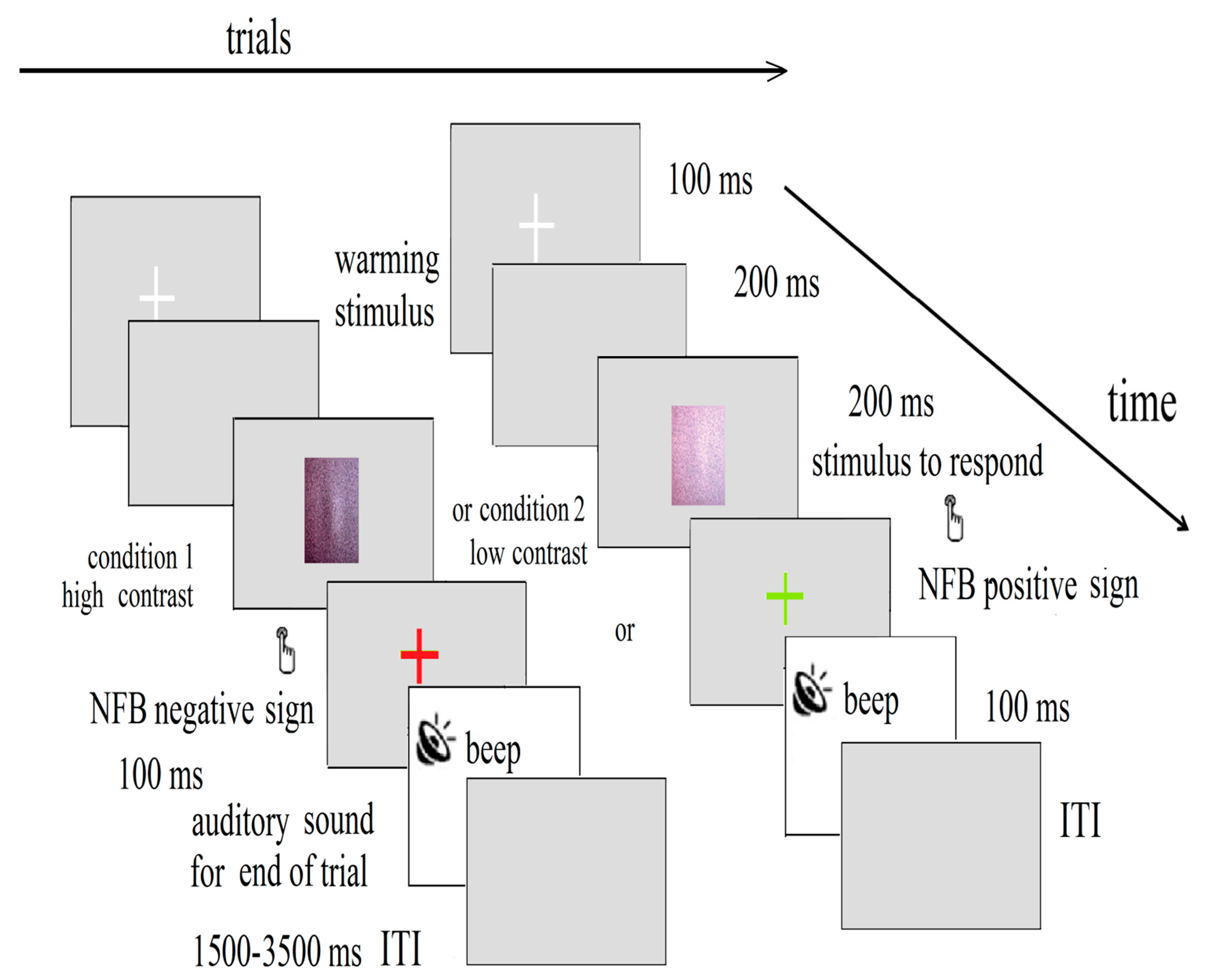
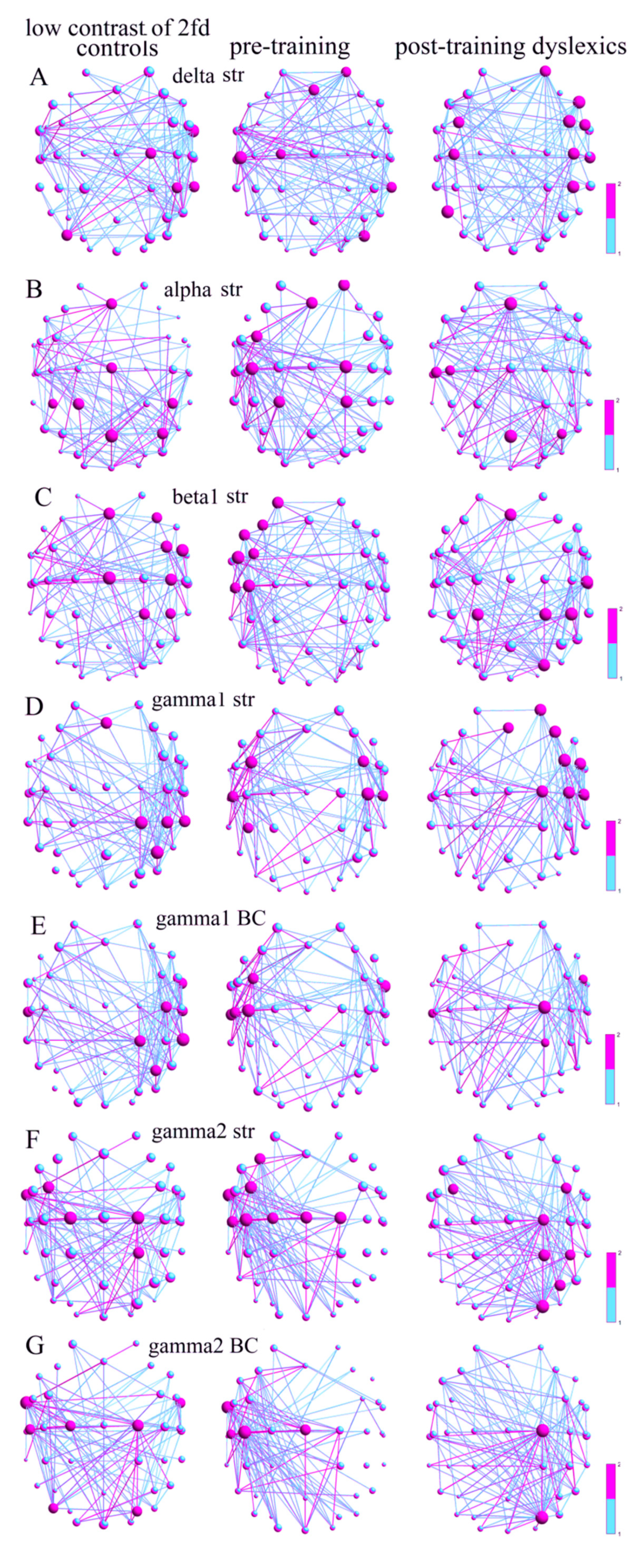
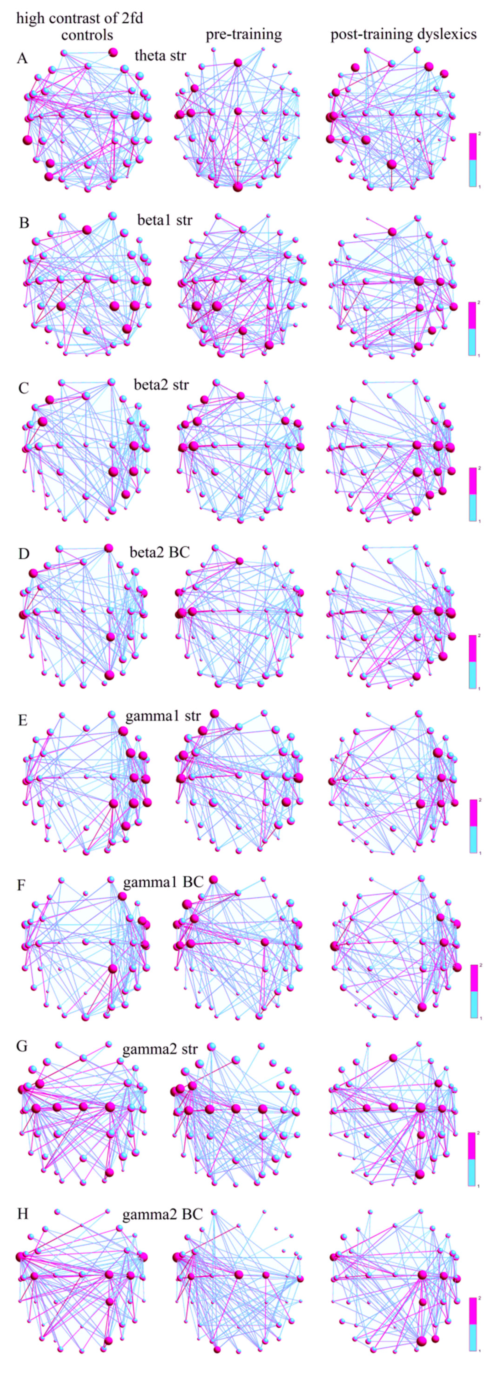
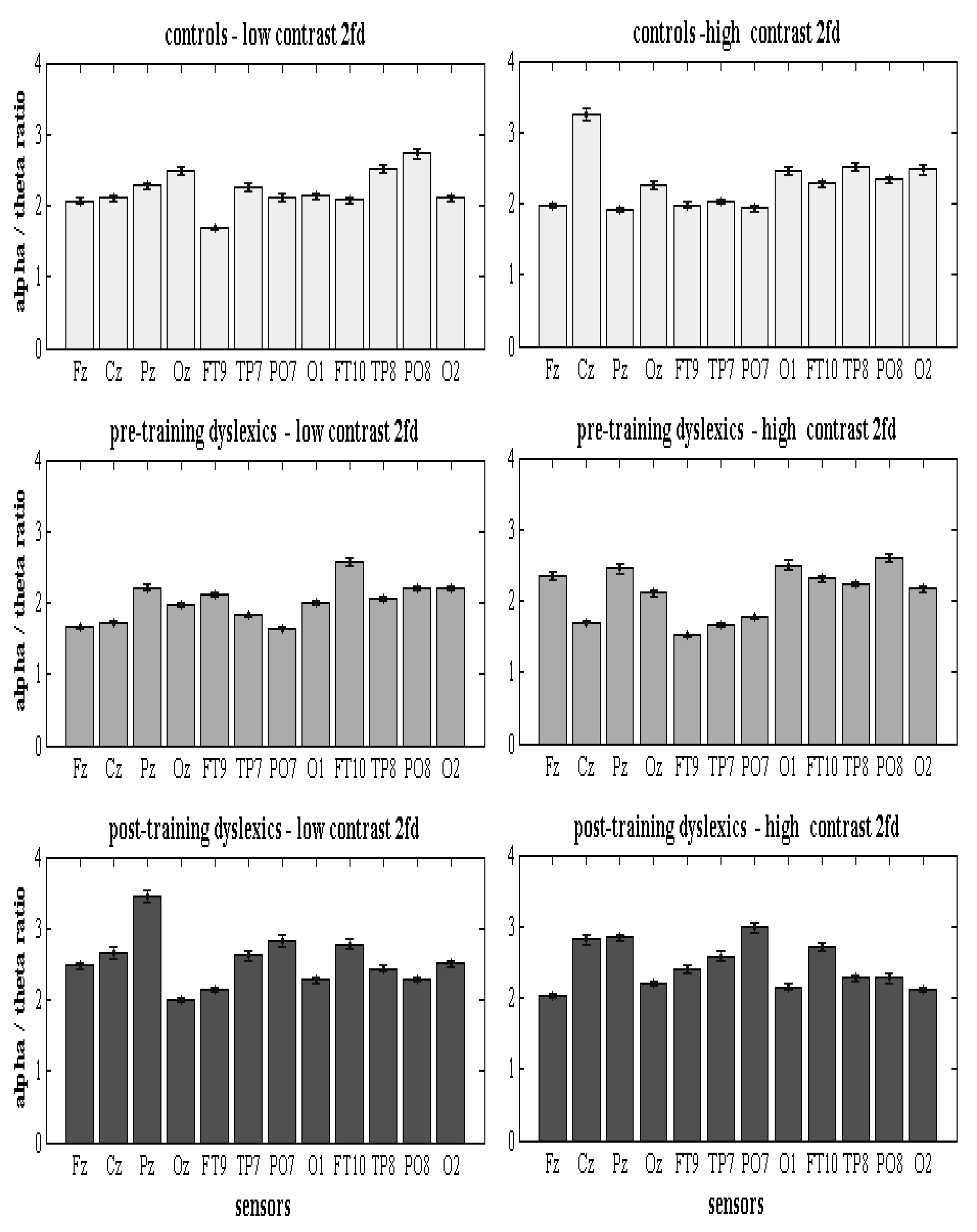
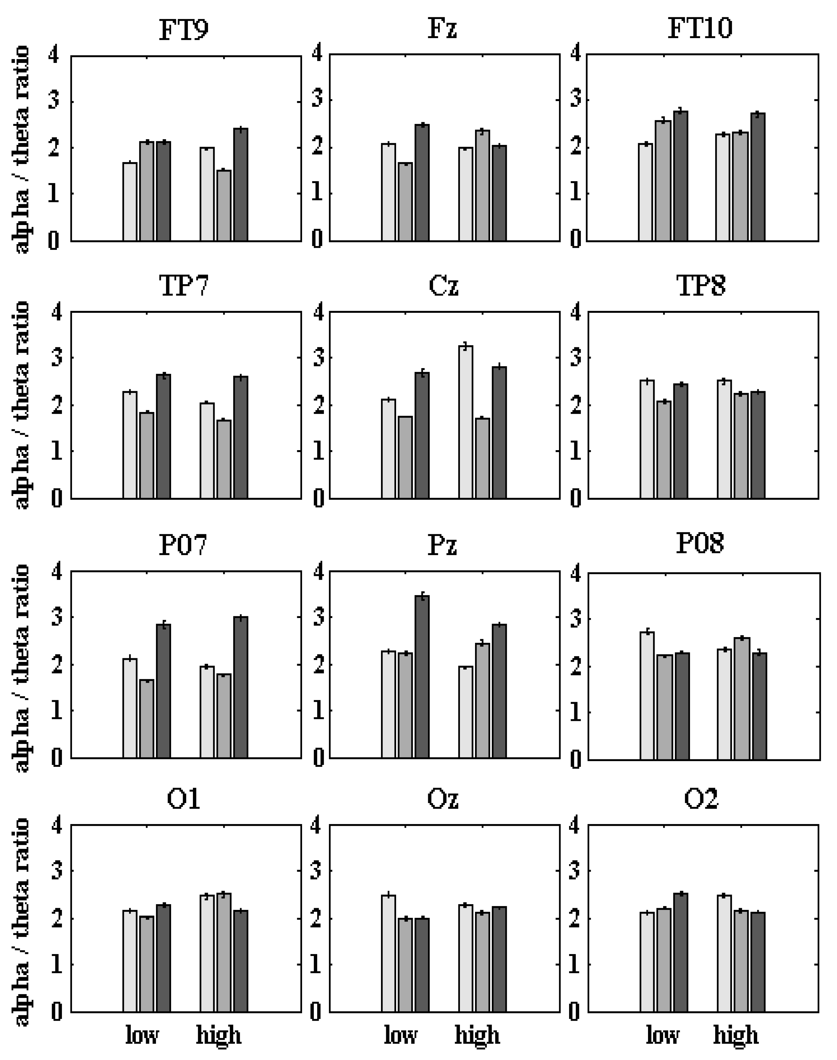
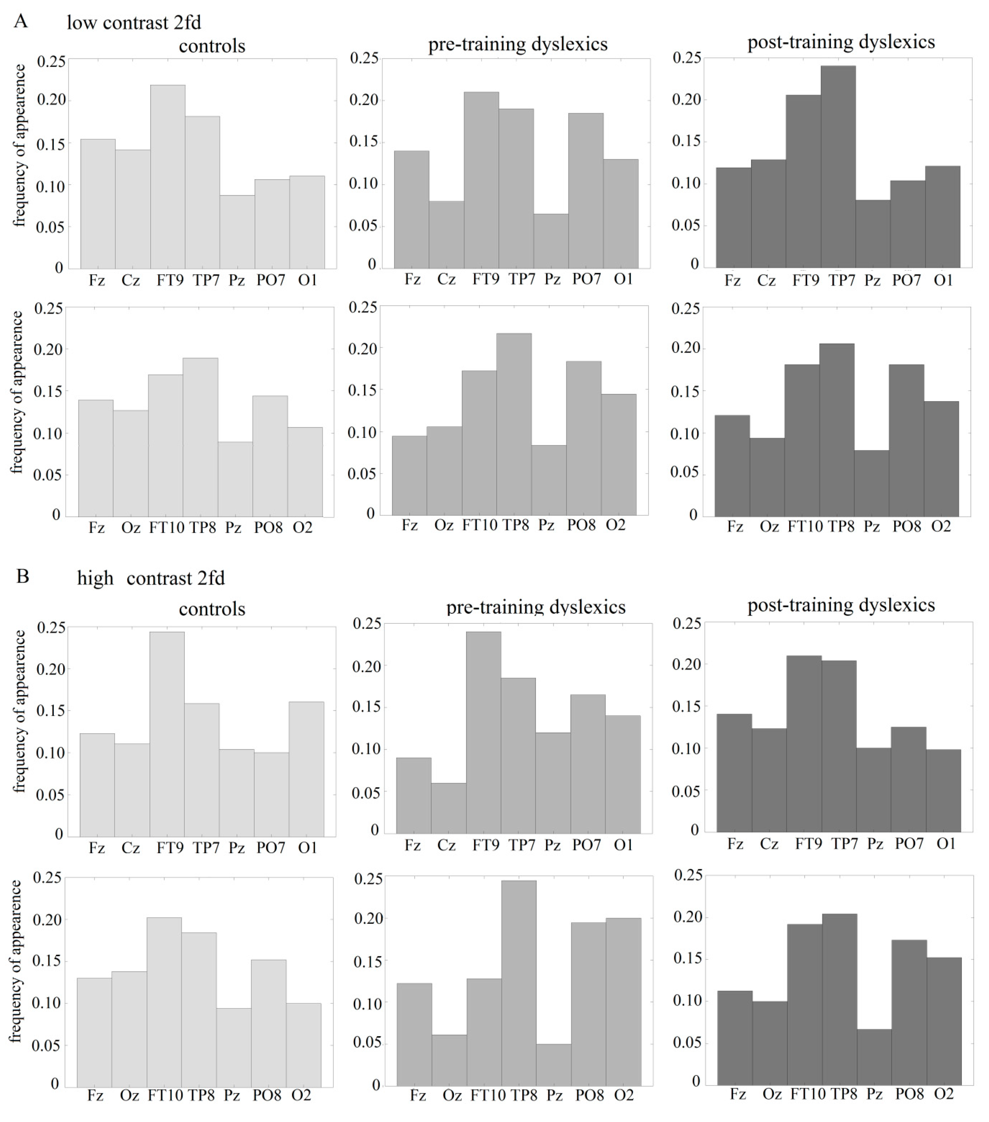
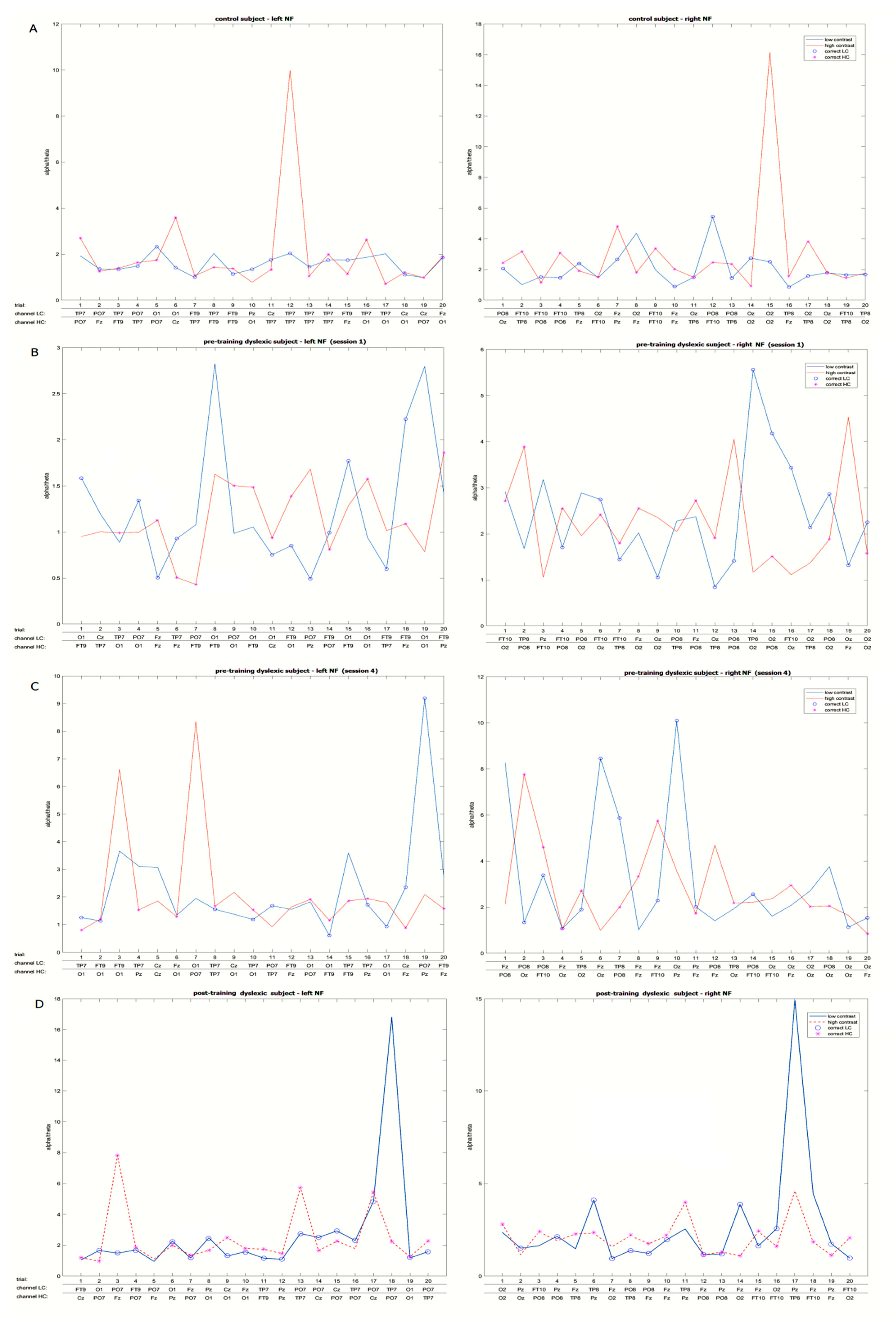
Table A1.
Nonparametric statistical comparisons of graph SWP metrics (significance threshold p < 0.025; strength: Str: strength; BC: betweenness centrality) of functional brain networks of control and dyslexic groups during low-contrast of 2fd for the frequencies: δ = 4; θ = 4.5–8; α = 8.5–13 β1= 13.5–20; β2 = 20.5–30; γ1 = 30.5–48; and γ2 = 52–70 Hz.
| Control | Pre- Dys | Post- Dys | Con/Pre- Dys | Con/Post- Dys | Pre-/Post- Dys | |||||
|---|---|---|---|---|---|---|---|---|---|---|
| Hubs | Hubs | Hubs | p | χ2 | p | χ2 | p | χ2 | ||
| δ | Str | FT10 C2 CP4 TP8 PO7 | AF4 Fz C1 C5 TP8 PO8 | AF4 F8 FC6 FC3-4 C3-4 T8 CP4 P7 | 0.021 | 5.29 | 0.640 | 0.21 | 0.052 | 3.75 |
| BC | FT9-10 C2 TP8 T7 PO7 P8 | AF3-4 FT9 Fz C5 T7-T8 TP8 PO4 P8 | AF4 F7-8 C3 T8 Oz | 0.067 | 3.33 | 0.868 | 0.03 | 0.227 | 1.45 | |
| θ | Str | F3 Fz C1 Cz CP3 CP4 TP8 | F3 C2 C4 CP4 P4 O1 | FT9 C5 Pz CP1 PO3 PO7 | 0.973 | 0.001 | 0.335 | 0.92 | 0.301 | 1.07 |
| BC | F7 Fz Oz PO3 FT10 | FT9-10 Fz Cz C2 Oz O2 | AF4 FT9-10 Pz T7 P4 PO7 | 0.195 | 1.67 | 0.611 | 0.26 | 0. 128 | 2.31 | |
| α | Str | Fz Cz CP1 CP3-4 Pz P4 | AF4 Fz FC3 C2 C3 CP1-2 | Fz C3 C5 Pz P4 | 0.023 | 5.16 | 0.085 | 2.96 | 0.938 | 0.01 |
| BC | FT9-10 Fz Pz PO8 T8 P8 Oz | FT9-10 C2 C3 P7 O1 | AF3 F7 Fz FT10 CP2 PO8 P8 | 0.591 | 0.28 | 0.611 | 0.19 | 0.941 | 0.01 | |
| β1 | Str | Fz F4 FC6 FC4 Cz C4 CP2 CP4 | AF3 F3 FC3 F7 FC5 C3 C5 | Fz C6 CP1-2 CP4 PO4 | 0.661 | 0.19 | 0.517 | 0.42 | 0.0005 | 12.06 |
| BC | Fz Cz C5 T7 PO4 P8 O1 | F7 C3 P7 | Fz C1 C5 T7 PO4 O1 | 0.994 | 3.9 × 10⁻⁵ | 0.986 | 0.0003 | 0.041 | 4.18 | |
| β2 | Str | FC6 C4 C5-6 P8 | Fz FC4 C3-4 C5-6 CP4 | Fz F4 FC4 Cz C1 C6 CP1 | 0.661 | 0.19 | 0.775 | 0.08 | 0.948 | 0.004 |
| BC | F7 Fz FT10 C2 T7 P8 | FT9-10 C3 C5 P7 | Fz F4 FT10 C1 C6 T8 | 0.994 | 3.9 × 10⁻⁵ | 0.205 | 1.61 | 0.208 | 1.57 | |
| γ1 | Str | Fz CP2 CP4 TP8 P4 | FC3-4 C4 C5-6 CP3 | AF4 F4 FC4 Fz FC6 C2 C4 C6 | 6.8 × 10⁻⁶ | 20.24 | 0.991 | 0.0001 | 0.0002 | 13.48 |
| BC | FT10 C4 T7-8 CP2 TP8 P4 | FC3 FT10 C3 C5 T7 | FC6 C2 T7 CP2 | 0.001 | 10.14 | 0.801 | 0.06 | 0.003 | 8.70 | |
| γ2 | Str | FC3 FT9 C1-2 CP2 | F3 FC3 FT9 Cz C1-C2 C3 C5 | FC3-4 C2 CP2 CP4 PO4 P4 | 2.0 × 10⁻¹³ | 54.02 | 0.012 | 6.22 | 1.0 × 10⁻¹⁵ | 64.35 |
| BC | FT9-10 C1-2 C5 PO4 PO7 | FT9 Cz C3 C5 | C2 PO4 | 8.8 × 10⁻⁶ | 19.76 | 0.004 | 8.17 | 1.4 × 10⁻¹⁰ | 41.22 | |
Table A2.
Nonparametric statistical comparisons of graph SWP metrics (p < 0.025; Str: strength; BC: betweenness centrality) of functional brain networks of control and dyslexic groups during high contrast of 2fd for the frequencies: δ = 4; θ = 4.5–8; α = 8.5–13; β1= 13.5–20; β2 = 20.5–30; γ1 = 30.5–48; and γ2 = 52–70 Hz.
| Control | Pre- Dys | Post- Dys | Con/Pre- Dys | Con/Post- Dys | Pre-/Post- Dys | |||||
|---|---|---|---|---|---|---|---|---|---|---|
| Hubs | Hubs | Hubs | p | χ2 | p | χ2 | p | χ2 | ||
| δ | Str | AF4 F4 F8 FC6 TP7 PO7-8 | C5 CP4 PO8 P8 | FC6 FT10 C2 C4 O1 | 0.138 | 2.19 | 0.068 | 3.30 | 0.402 | 0.70 |
| BC | FT9 F4 T7 CP2 PO7-8 | FC3 FT10 C5 T7 P4 PO8 P7 | F7 FT9-10 C6 PO4 PO8 O1 | 0.923 | 0.009 | 0.975 | 0.001 | 0.971 | 0.001 | |
| θ | Str | AF4 C4 P3 TP7 PO7 | FC3 Fz Cz C3 C5 Oz | F3-4 FC5 F8 C5 T7 CP1 Pz TP7 | 1.7 × 10⁻⁵ | 18.51 | 0.066 | 3.36 | 0.185 | 1.75 |
| BC | FT9-10 T7 PO4 PO7 P8 | PO7 Oz O1 | F4 T7 PO8 O2 | 0.339 | 4.49 | 0.067 | 3.33 | 0.755 | 0.09 | |
| α | Str | Fz Cz Pz C2 | AF4 F3 FC5 Fz C3 C5 CP1 | FC4 Cz CP1 C2 P4 PO4 | 0.511 | 0.43 | 0.108 | 2.57 | 0.029 | 4.73 |
| BC | FT9 Cz C2 TP7 PO3-4 PO8 P8 | FT9-10 Fz T7 PO4 PO8 Oz O1 | FT9 F4 CP1 P7 PO4 PO8 O2 | 0.655 | 0.19 | 0.394 | 0.72 | 0.605 | 0.26 | |
| β1 | Str | Fz CP1-2 C6 CP4 P4 | CP1 Pz CP3 PO4 | Fz C2 C4 CP2 TP8 P4 PO4 | 0.283 | 1.14 | 0.005 | 7.61 | 0.0002 | 13.29 |
| BC | Cz PO8 T7 P7 | T7 PO4 PO7 P7 | F7 Fz C2 T8 PO3-4 | 0.716 | 0.13 | 0.070 | 3.28 | 0.032 | 4.59 | |
| β2 | Str | F3 FC3 C4 CP2 CP4 P4 | F3 FC3-4 FC5-6 Fz C3 C5-6 | FC6 C2 C4 C6 CP2 CP4 TP8 PO4 P4 P8 | 0.101 | 2.67 | 7.1 × 10⁻⁶ | 20.16 | 1.8 × 10⁻⁹ | 36.14 |
| BC | AF4 F7 FT10 T7 CP2 PO4 | Fz FT9-10 C3 C5 T7 | C2 C4 C6 T8 TP8 PO4 P8 | 0.001 | 9.72 | 0.027 | 4.88 | 1.3 × 10⁻⁶ | 23.43 | |
| γ1 | Str | F4 FC4 FC6 C4 C6 CP2 CP4 TP8 P4 | AF3 F3 FC5 C5-6 CP4 | FC4 C4 CP2 CP4 TP8 T7 | 0.009 | 6.67 | 0.012 | 6.26 | 5.9 × 10⁻⁶ | 20.51 |
| BC | F4 FC6 FT10 C6 CP2 | AF3 F7 FC3 FT9-10 C2 C3 C5 | FC4 FT10 T7 C4 TP8 PO4 | 0.013 | 6.07 | 0.009 | 6.65 | 6.2 × 10⁻⁶ | 20.42 | |
| γ2 | Str | FC3 FT9 Cz C1-2 C3 PO4 | FC3 FC5 FT9 Cz C1-2 C3 | Fz FC4 Cz C1-2 C4 CP2 PO4 | 1.7 × 10⁻¹⁷ | 27.29 | 0.001 | 10.65 | 8.6 × 10⁻¹³ | 51.14 |
| BC | FT9-10 C2 C3-4 CP2 PO4 | FT9 Cz C2 C3 T8 O1 | FT9 C2 C4 T8 CP2 PO4 PO8 | 0.003 | 8.69 | 0.009 | 6.78 | 4.5 × 10⁻⁷ | 25.48 | |
Table A3.
Nonparametric statistical comparisons (p < 0.05) of the α/θ scores between the sensors of the groups during contrast discrimination of LSF illusion (2fd).
Table A3.
Nonparametric statistical comparisons (p < 0.05) of the α/θ scores between the sensors of the groups during contrast discrimination of LSF illusion (2fd).
| α/θ Scores | Con | Pre-D | Post-D | Con/Pre-D | Con/Post-D | Pre-/Post-D | |||
|---|---|---|---|---|---|---|---|---|---|
| Mean ± s.e. | Mean ± s.e. | Mean ± s.e. | p | χ2 | p | χ2 | p | χ2 | |
| Low-contrast | |||||||||
| Fz | 2.06 ± 0.04 | 1.65 ± 0.02 | 2.47 ± 0.05 | 1.9 × 10⁻¹⁰ | 40.8 | 2.4 × 10⁻¹¹ | 44.6 | 2.7 × 10−40 | 176.6 |
| Cz | 2.10 ± 0.04 | 1.73 ± 0.01 | 2.66 ± 0.08 | 0.0010 | 10.6 | 0.0131 | 6.2 | 5.2 × 10⁻⁴ | 12.1 |
| Pz | 2.27 ± 0.05 | 2.21 ± 0.04 | 3.44 ± 0.08 | 0.0039 | 8.34 | 3.3 × 10−40 | 176.2 | 3.7 × 10⁻³² | 139.4 |
| Oz | 2.48 ± 0.06 | 1.97 ± 0.04 | 2.00 ± 0.03 | 4.0 × 10⁻¹⁷ | 70.8 | 7.2 × 10⁻⁶ | 20.2 | 2.0 × 10⁻¹¹ | 44.9 |
| FT9 | 1.68 ± 0.02 | 2.12 ± 0.03 | 2.13 ± 0.03 | 1.3 × 10⁻²² | 95.7 | 4.9 × 10⁻³³ | 143.4 | 0.303 | 1.06 |
| TP7 | 2.26 ± 0.05 | 1.82 ± 0.02 | 2.62 ± 0.07 | 1.9 × 10⁻⁵ | 18.3 | 7.2 × 10⁻¹⁰ | 37.9 | 2.2 × 10⁻²⁴ | 103.8 |
| PO7 | 2.12 ± 0.05 | 1.64 ± 0.02 | 2.82 ± 0.08 | 2.7 × 10⁻⁹ | 35.4 | 2.4 × 10⁻¹⁵ | 62.7 | 3.7 × 10−38 | 166.8 |
| O1 | 2.13 ± 0.04 | 2.01± 0.03 | 2.27 ± 0.05 | 0.4743 | 0.51 | 0.0339 | 4.5 | 0.193 | 1.71 |
| FT10 | 2.08 ± 0.04 | 2.57 ± 0.06 | 2.77 ± 0.07 | 1.9 × 10⁻¹⁴ | 58.6 | 4.7 × 10⁻¹¹ | 43.3 | 0.79 | 0.07 |
| TP8 | 2.50 ± 0.06 | 2.06 ± 0.03 | 2.43 ± 0.04 | 5.1 × 10⁻⁴ | 12.1 | 8.8 × 10⁻⁴ | 11.1 | 1.2 × 10⁻⁹ | 36.9 |
| PO8 | 2.73 ± 0.07 | 2.21 ± 0.03 | 2.28 ± 0.03 | 6.1 × 10⁻⁷ | 24.9 | 0.202 | 1.63 | 0.0015 | 10.1 |
| O2 | 2.10 ± 0.03 | 2.20 ± 0.03 | 2.50 ± 0.04 | 0.1045 | 2.64 | 3.4 × 10⁻¹⁸ | 75.3 | 1.9 × 10⁻¹¹ | 45.1 |
| High-contrast | |||||||||
| Fz | 1.97 ± 0.03 | 2.34 ± 0.06 | 2.02 ± 0.03 | 2.4 × 10⁻⁴ | 13.5 | 6.2 × 10⁻⁴ | 11.7 | 2.5 × 10⁻⁹ | 35.5 |
| Cz | 3.24 ± 0.09 | 1.70 ± 0.02 | 2.81 ± 0.07 | 5.6 × 10−49 | 216.4 | 0.002 | 9.5 | 3.5 × 10−38 | 166.9 |
| Pz | 1.92± 0.02 | 2.44 ± 0.06 | 2.84 ± 0.04 | 2.0 × 10⁻⁶ | 22.6 | 9.9 × 10−62 | 274.9 | 1.8 × 10⁻²⁸ | 122.5 |
| Oz | 2.26 ± 0.05 | 2.10 ± 0.03 | 2.21 ± 0.03 | 0.215 | 1.54 | 0.002 | 9.77 | 0.008 | 7.02 |
| FT9 | 1.98 ± 0.04 | 1.51 ± 0.02 | 2.40 ± 0.06 | 1.8 × 10⁻¹⁸ | 76.9 | 8.0 × 10⁻⁸ | 28.8 | 4.4 × 10−45 | 198.5 |
| TP7 | 2.04 ± 0.03 | 1.66 ± 0.02 | 2.58 ± 0.06 | 1.4 × 10⁻²⁸ | 122.9 | 6.7 × 10⁻⁴ | 11.6 | 1.9 × 10−42 | 186.4 |
| PO7 | 1.93 ± 0.03 | 1.76 ± 0.02 | 2.98 ± 0.08 | 1.4 × 10⁻⁷ | 27.7 | 2.0 × 10⁻²² | 94.9 | 8.6 × 10−40 | 174.3 |
| O1 | 2.45 ± 0.06 | 2.49 ± 0.07 | 2.15 ± 0.04 | 0.062 | 3.49 | 0.040 | 4.21 | 1.2 × 10⁻⁸ | 32.4 |
| FT10 | 2.27 ± 0.04 | 2.30 ± 0.04 | 2.70 ± 0.06 | 0.032 | 4.61 | 5.3 × 10⁻⁴ | 12.0 | 3.2 × 10⁻⁹ | 35.1 |
| TP8 | 2.50 ± 0.06 | 2.23 ± 0.03 | 2.27 ± 0.04 | 0.007 | 7.30 | 0.048 | 4.61 | 0.613 | 0.26 |
| PO8 | 2.33 ± 0.04 | 2.59 ± 0.05 | 2.27 ± 0.06 | 8.8 × 10⁻⁵ | 15.4 | 8.6 × 10⁻⁶ | 19.8 | 1.2 × 10⁻¹⁹ | 82.2 |
| O2 | 2.47 ± 0.06 | 2.16 ± 0.04 | 2.12 ± 0.03 | 4.6 × 10⁻⁵ | 16.6 | 9.4 × 10⁻²⁰ | 82.7 | 0.12 | 2.5 |
Figure A1.
Averaged α/θ scores for Fz, Cz, Oz, FT9, FT10, TP7, TP8, Pz, PO7, PO8, O1, and O2 for each group (Con: light gray; preD: middle gray; postD: dark gray) and condition (low-contrast; high-contrast), separately.
Figure A1.
Averaged α/θ scores for Fz, Cz, Oz, FT9, FT10, TP7, TP8, Pz, PO7, PO8, O1, and O2 for each group (Con: light gray; preD: middle gray; postD: dark gray) and condition (low-contrast; high-contrast), separately.

Figure A2.
Frequencies of appearances of the z-NF sensors for each group and condition represented separately.
Figure A2.
Frequencies of appearances of the z-NF sensors for each group and condition represented separately.

Figure A3.
The online appearances of the qEEG z-NF sensors during session recording (x-axis, number trials, channel’s name) for individual (A) control subject; (B) first session for preD subject; (C) fourth session for preD subject; (D) last session for postD subject, for left and right hemisphere, separately represented discrimination of low-contrast sinusoidal grating: blue line; high-contrast discrimination: red line; circles and stars mark the correct trials. During the neurofeedback session, the qEEG z-NF α/θ scores lower than 1 correspond to a red color cross on the screen, and those α/θ scores higher than 1 correspond to a green color mark on the screen.

Table A4.
Comparisons of the limitations and advantages of the training programs for developmental dyslexia in the literature, which combines the EEG-channel neurofeedback and multisensory learning methods [54,126].
| Groups | Present Study | (qEEG z-NF | -VT) | Other Study | (AutoTrainBrain) | [54,126] |
|---|---|---|---|---|---|---|
| Features | Advantages | Disadvantages | Differences | Advantages | Disadvantages | Differences |
| Control group | Typically reading children | No VT | Size of group (36) | Multisensory learning with alphabet letters | Children with pure dyslexia | Size of group (14) |
| Pre- qEEG z-NF | Functional connectivity (neural network) in all frequency bands | Pre- qEEG z-NF, post- qEEG z-NF | Complexity (entropy), coherence powers of all frequency bands | |||
| qEEG z-NF-alpha/theta | qEEG z-NF-theta | |||||
| Experimental group | Developmental dyslexia | Size of group (72) | Multisensory learning | Dyslexia combined with comorbid cases | Size of group (16) | |
| VT directed to specific visual deficits (deficits of magnocellular pathway and its functioning; parvocellular pathway; temporal cortex; visual-spatial attention) | No chosen individual parameters for training the specific visual deficits | Visual, auditory, and reading tasks in pretraining period; visual and reading tasks in postperiod | Multisensory learning | No specific training; | Common reading tasks in pre- and post-training periods | |
| Pre-NF, post-NF | NF-specific magnocellular task | Pre-qEEG z-NF, post- qEEG z-NF | qEEG z-NF audio-visual word task | |||
| More flexible 12- qEEG z-NF system | Stimulates compensatory mechanisms in the hemisphere’s functioning | Less flexible 14- qEEG z-NF | Improved the cognitive abilities | |||
| Pre- qEEG z-NF, Post- qEEG z-NF | 3-month duration between pre- and post- EEG measurements | Pre- qEEG z-NF, post- qEEG z-NF | 6-month duration between pre- and post- EEG measurements | |||
| 12 pre- and post- qEEG z-NF | 360 sessions of VT training during 12 consecutive weeks (11,600 trials) | 60 sessions of qEEG z-NF training during 12 consecutive weeks | ||||
| Reading assessments [55] | Reading assessments [126] |
References
- Lawrence, E.J.; Su, L.; Barker, G.J.; Medford, N.; Dalton, J.; Williams, S.C.R.; Birbaumer, N.; Veit, R.; Ranganatha, S.; Bodurka, J.; et al. Self-regulation of the anterior insula: Reinforcement learning using real-time fMRI neurofeedback. Neuroimage 2014, 88, 113–124. [Google Scholar] [CrossRef]
- Coben, R.; Linden, M.; Myers, T.E. Neurofeedback for autistic spectrum disorder: A review of the literature. Appl. Psychophysiol. Biofeedback 2010, 35, 83–105. [Google Scholar] [CrossRef] [PubMed]
- Lofthouse, N.; Hendren, R.; Hurt, E.; Arnold, L.E.; Butter, E. A review of complementary and alternative treatments for autism spectrum disorders. Autism Res. Treat. 2012, 2012, 870391. [Google Scholar] [CrossRef] [PubMed]
- Zoefel, B.; Huster, R.J.; Herrmann, C.S. Neurofeedback training of the upper α frequency band in EEG improves cognitive performance. Neuroimage 2011, 54, 1427–1431. [Google Scholar] [CrossRef] [PubMed]
- Angelakis, E.; Stathopoulou, S.; Frymiare, J.L.; Green, D.L.; Lubar, J.F.; Kounios, J. EEG Neurofeedback: A Brief Overview and an Example of Peak Alpha Frequency Training for Cognitive Enhancement in the Elderly. Clin. Neuropsychol. 2007, 21, 110–129. [Google Scholar] [CrossRef]
- Pérez-Elvira, R.; Oltra-Cucarella, J.; Carrobles, J.A. Effects of quantitative electroencephalogram normalization using 4-channel live z-score training neurofeedback for children with learning disabilities: Preliminary data. Behav. Psychol. Psicol. Conduct. 2021, 29, 191–206. [Google Scholar] [CrossRef]
- Wigton, N.L.; Krigbaum, G. Attention, executive function, behavior, and electrocortical function, significantly improved with 19-channel z-score neurofeedback in a clinical setting: A pilot study. J. Atten. Disord. 2015, 23, 398–408. [Google Scholar] [CrossRef]
- Collura, T. Live z-score Neurofeedback. Biofeedback 2016, 44, 212–217. [Google Scholar] [CrossRef]
- Smetanin, N.; Lebedev, M.A.; Ossadtchi, A. Towards zero-latency neurofeedback. bioRxiv 2018, 424846. [Google Scholar] [CrossRef] [Green Version]
- Tang, Y.Y.; Posner, M.I. Training brain networks and states. Trends Cogn. Sci. 2014, 18, 345–350. [Google Scholar] [CrossRef]
- Petersen, S.E.; Posner, M.I. The attention system of the human brain: 20 years after. Annu. Rev. Neurosci. 2012, 35, 73–89. [Google Scholar] [CrossRef] [PubMed] [Green Version]
- Jensen, C.G.; Vangkilde, S.; Frokjaer, V.; Hasselbalch, S.G. Mindfulness training affects attention or is it attentional effort? J. Exp. Psychol Gen. 2012, 141, 106–123. [Google Scholar] [CrossRef] [PubMed] [Green Version]
- Cattinelli, I.; Borghese, N.A.; Gallucci, M.; Paulesu, E. Reading the reading brain: A new meta-analysis of functional imaging data on reading. J. Neurolinguistics 2013, 26, 214–238. [Google Scholar] [CrossRef]
- Cao, F.; Yan, X.; Wang, Z.; Liu, Y.; Wang, J.; Spray, G.J.; Deng, Y. Neural signatures of phonological deficits in Chinese developmental dyslexia. Neuroimage 2017, 146, 301–311. [Google Scholar] [CrossRef] [PubMed]
- Buchweitz, A.; Costa, A.C.; Toazza, R.; de Moraes, A.B.; Cara, V.M.; Esper, N.B.; Aguzzoli, C.; Gregolim, B.; Dresch, L.F.; Soldatelli, M.D.; et al. Decoupling of the occipitotemporal cortex and the brain’s default-mode network in dyslexia and a role for the cingulate cortex in good readers: A brain imaging study of Brazilian children. Dev. Neuropsychol. 2019, 44, 146–157. [Google Scholar] [CrossRef]
- Bosch-Bayard, J.; Peluso, V.; Galan, L.; Valdes Sosa, P.; Chiarenza, G. Clinical and Electrophysiological Differences between Subjects with Dysphonetic Dyslexia and Non-Specific Reading Delay. Brain Sci. 2018, 8, 172. [Google Scholar] [CrossRef] [Green Version]
- Roca-Stappung, M.; Fernández, T.; Bosch-Bayard, J.; Harmony, T.; Ricardo-Garcell, J. Electroencephalographic characterization of subgroups of children with learning disorders. PLoS ONE 2017, 12, e0179556. [Google Scholar] [CrossRef] [Green Version]
- Kaiser, D.A.; Othmer, S. Effect of neurofeedback on variables of attention in a large multi-center trial. J. Neurother. 2000, 4, 5–15. [Google Scholar] [CrossRef] [Green Version]
- Medici, D. Neurofeedback versus pharmacological intervention in the treatment of childhood attention-deficit/hyperactivity disorder (ADHD), First Spanish clinical neuropsychological study. Am. J. Appl. Psychol. 2018, 7, 57. [Google Scholar] [CrossRef] [Green Version]
- Ochi, Y.; Laksanasopin, T.; Kaewkamnerdpong, B.; Thanasuan, K. Neurofeedback game for attention training in adults. In Proceedings of the 10th Biomedical Engineering International Conference (BMEiCON), Hokkaido, Japan, 31 August–2 September 2017; pp. 1–5. [Google Scholar]
- Rastegar, N.; Dolatshahi, B.; Rezaee Dogahe, E. The effect of neurofeedback training on increasing sustained attention in veterans with posttraumatic stress disorder. Pract. Clin. Psychol. 2016, 4, 97–104. [Google Scholar] [CrossRef] [Green Version]
- Wang, J.-R.; Hsieh, S. Neurofeedback training improves attention and working memory performance. Clin. Neurophysiol. 2013, 124, 2406–2420. [Google Scholar] [CrossRef] [PubMed]
- Gasser, T.; Rousson, V.; Gasser, U.S. EEG power and coherence in children with educational problems. J. Clin. Neurophysiol. 2003, 20, 273–282. [Google Scholar] [CrossRef]
- Dickinson, A.; DiStefano, C.; Senturk, D.; Jeste, S.S. Peak alpha frequency is a neural marker of cognitive function across the autism spectrum. Eur. J. Neurosci. 2018, 47, 643–651. [Google Scholar] [CrossRef] [PubMed] [Green Version]
- Klimesch, W. EEG alpha and theta oscillations reflect cognitive and memory performance: A review and analysis. Brain Res. Rev. 1999, 29, 169–195. [Google Scholar] [CrossRef]
- Bazanova, O.M. Alpha EEG Activity Depends on the Individual Dominant Rhythm Frequency. J. Neurother. 2012, 16, 270–284. [Google Scholar] [CrossRef]
- Grandy, T.H.; Werkle-Bergner, M.; Chicherio, C.; Lövdén, M.; Schmiedek, F.; Lindenberger, U. Individual alpha peak frequency is related to latent factors of general cognitive abilities. NeuroImage 2013, 79, 10–18. [Google Scholar] [CrossRef] [PubMed] [Green Version]
- Niedermeyer, E.; Lopes da Silva, F.H. Electroencephalography: Basic Principles, Clinical Applications, and Related Fields, 5th ed.; Lippincott Williams & Wilkins: London, UK, 2005; ISBN 978-0-7817-5126-1. [Google Scholar]
- Fernández, T.; Bosch-Bayard, J.; Harmony, T.; Caballero, M.I.; Díaz-Comas, L.; Galán, L.; Ricardo-Garcell, J.; Aubert, E.; Otero-Ojeda, G. Neurofeedback in Learning Disabled Children: Visual versus Auditory Reinforcement. Appl. Psychophysiol. Biofeedback 2016, 41, 27–37. [Google Scholar] [CrossRef] [PubMed]
- Arns, M. EEG-Based Personalized Medicine in ADHD: Individual Alpha Peak Frequency as an Endophenotype Associated with Nonresponse. J. Neurother. 2012, 16, 123–141. [Google Scholar] [CrossRef]
- Güntensperger, D.; Thüring, C.; Kleinjung, T.; Neff, P.; Meyer, M. Investigating the Efficacy of an Individualized α/δ Neurofeedback Protocol in the Treatment of Chronic Tinnitus. Neural Plast. 2019, 2019, 3540898. [Google Scholar] [CrossRef] [Green Version]
- Albarrán-Cárdenas, L.; Silva-Pereyra, J.; Martínez-Briones, B.J.; Bosch-Bayard, J.; Fernández, T. Neurofeedback effects on EEG connectivity in children with reading disorder: I. Coherence. Preprints 2021, 2021080427. [Google Scholar] [CrossRef]
- Martínez-Briones, B.J.; Bosch-Bayard, J.; Biscay-Lirio, R.J.; Silva-Pereyra, J.; Albarrán-Cárdenas, L.; Fernández, T. Effects of neurofeedback on the working memory of children with learning disorders—An eeg power-spectrum analysis. Brain Sci. 2021, 11, 957. [Google Scholar] [CrossRef] [PubMed]
- Van Dijk, H.; Schoffelen, J.M.; Oostenveld, R.; Jensen, O. Prestimulus oscillatory activity in the alpha band predicts visual discrimination ability. J. Neurosci. 2008, 28, 1816–1823. [Google Scholar] [CrossRef] [PubMed] [Green Version]
- Gola, M.; Magnuski, M.; Szumska, I.; Wróbel, A. EEG beta-band activity is related to attention and attentional deficits in the visual performance of elderly subjects. Int. J. Psychophysiol. 2013, 89, 334–341. [Google Scholar] [CrossRef] [PubMed]
- Phipps-Nelson, J.; Redman, J.R.; Rajaratnam, S.M. Temporal profile of prolonged, night-time driving performance: Breaks from driving temporarily reduce time-on-task fatigue but not sleepiness. J. Sleep Res. 2011, 20, 404–415. [Google Scholar] [CrossRef]
- Wascher, E.; Rasch, B.; Sänger, J.; Hoffmann, S.; Schneider, D.; Rinkenauer, G.; Heuer, H.; Gutberlet, I. Frontal theta activity reflects distinct aspects of mental fatigue. Biol. Psychol. 2014, 96, 57–65. [Google Scholar] [CrossRef]
- Henson, R.; Rugg, M. Neural response suppression, hemodynamic repetition effects, and behavioural priming. Neuropsychologia 2003, 41, 263–270. [Google Scholar] [CrossRef]
- Maksimenko, V.; Kuc, A.; Frolov, N.S.; Hramov, A.; Pisarchik, A.; Lebedev, M. Neuronal adaptation in the course of the prolonged task improves visual stimuli processing. bioRxiv 2020. [CrossRef] [Green Version]
- Harmony, T.; Hinojosa, G.; Marosi, E.; Becker, J.; Rodriguez, M.; Reyes, A.; Rocha, C. Correlation between EEG Spectral Parameters and an Educational Evaluation. Int. J. Neurosci. 1990, 54, 147–155. [Google Scholar] [CrossRef]
- Jäncke, L.; Alahmadi, N. Resting-State EEG in Children with Learning Disabilities. Clin. EEG Neurosci. 2016, 47, 24–36. [Google Scholar] [CrossRef]
- Fonseca, L.C.; Tedrus, G.M.A.S.; Chiodi, M.G.; Cerqueira, J.N.; Tonelotto, J.M.F. Quantitative EEG in Children with Learning Disabilities: Analysis of Band Power. Arq. Neuropsiquiatr. 2006, 64, 376–378. [Google Scholar] [CrossRef] [Green Version]
- Coben, R.; Wright, E.K.; Decker, S.L.; Morgan, T. The impact of coherence neurofeedback on reading delays in learning disabled children: A randomized controlled study. NeuroRegulation 2015, 2, 168. [Google Scholar] [CrossRef] [Green Version]
- Murias, M.; Swanson, J.M.; Srinivasan, R. Functional Connectivity of Frontal Cortex in Healthy and ADHD Children Reflected in EEG Coherence. Cereb. Cortex 2007, 17, 1788–1799. [Google Scholar] [CrossRef] [PubMed] [Green Version]
- Dhar, M.; Been, P.H.; Minderaa, R.B.; Althaus, M. Reduced Interhemispheric Coherence in Dyslexic Adults. Cortex 2010, 46, 794–798. [Google Scholar] [CrossRef] [PubMed]
- Marosi, E.; Harmony, T.; Reyes, A.; Bernal, J.; Fernández, T.; Guerrero, V.; Rodríguez, M.; Silva, J.; Yáñez, G.; Rodríguez, H. A Follow-up Study of EEG Coherences in Children with Different Pedagogical Evaluations. Int. J. Psychophysiol. 1997, 25, 227. [Google Scholar] [CrossRef]
- Leisman, G. Coherence of Hemispheric Function in Developmental Dyslexia. Brain Cogn. 2002, 48, 425–431. [Google Scholar]
- Au, A.; Ho, G.S.; Choi, E.W.; Leung, P.; Waye, M.M.; Kang, K.; Au, K.-Y. Does it help to train attention in dyslexic children: Pilot case studies with a ten-session neurofeedback program. Int. J. Disabil. Hum. Dev. 2014, 13, 45–54. [Google Scholar] [CrossRef]
- Breteler, M.H.; Arns, M.; Peters, S.; Giepmans, I.; Verhoeven, L. Improvements in spelling after qEEG-based neurofeedback in dyslexia: A randomized controlled treatment study. Appl. Psychophysiol. Biofeedback 2010, 35, 5–11. [Google Scholar] [CrossRef] [Green Version]
- Nazari, M.A.; Mosanezhad, E.; Hashemi, T.; Jahan, A. The effectiveness of neurofeedback training on EEG coherence and neuropsychological functions in children with reading disability. Clin. EEG Neurosci. 2012, 43, 315–322. [Google Scholar] [CrossRef]
- Klimesch, W.; Doppelmayr, M.; Wimmer, H.; Gruber, W.; Röhm, D.; Schwaiger, J.; Hutzler, F. Alpha and beta band power changes in normal and dyslexic children. Clin. Neurophysiol. 2001, 112, 1186–1195. [Google Scholar] [CrossRef]
- Rippon, G.; Brunswick, N. Trait and state EEG indices of information processing in developmental dyslexia. Int. J. Psychophysiol. 2000, 36, 251–265. [Google Scholar] [CrossRef]
- Arns, M.; Peters, S.; Breteler, R.; Verhoeven, L. Different brain activation patterns in dyslexic children: Evidence from EEG power and coherence patterns for the double-deficit theory of dyslexia. J. Integr. Neurosci. 2007, 6, 175–190. [Google Scholar] [CrossRef] [PubMed]
- Eroğlu, G.; Teber, S.; Ertürk, K.; Kırmızı, M.; Ekici, B.; Arman, F.; Balcisoy, S.; Özcan, Y.Z.; Çetin, M. A mobile app that uses neurofeedback and multi-sensory learning methods improve reading abilities in dyslexia: A pilot study. Appl. Neuropsychol. Child 2021, 1–11. [Google Scholar] [CrossRef] [PubMed]
- Dushanova, J.; Lalova, Y.; Kalonkina, A. Protocol for Visual Intervention of Developmental Dyslexia. In Proceedings of the 4th International Conference on Research in Humanities and Social Sciences, Milan, Italy, 7–9 May 2021; pp. 1–19. [Google Scholar]
- Rajabi, S.; Pakize, A.; Moradi, N. Effect of combined neurofeedback and game-based cognitive training on the treatment of ADHD: A randomized controlled study. Appl. Neuropsychol. Child 2020, 9, 193–205. [Google Scholar] [CrossRef] [PubMed]
- Tu, W.; Ma, Z.; Zhang, N. Brain network reorganization after a targeted attack at a hub region. NeuroImage 2021, 237, 118219. [Google Scholar] [CrossRef]
- Martin, A.; Schurz, M.; Kronbichler, M.; Richlan, F. Reading in the Brain of Children and Adults: A Meta-Analysis of 40 Functional Magnetic Resonance Imaging Studies. Hum. Brain Mapp. 2015, 36, 1963–1981. [Google Scholar] [CrossRef] [PubMed]
- Taskov, T.; Dushanova, J. Reading-network in developmental dyslexia before and after visual training. Symmetry 2020, 12, 1842. [Google Scholar] [CrossRef]
- Taskov, T.; Dushanova, J. Functional connectivity in developmental dyslexia during speed discrimination. Symmetry 2021, 13, 749. [Google Scholar] [CrossRef]
- Raichev, P.; Geleva, T.; Valcheva, M.; Rasheva, M.; Raicheva, M. Protocol on neurological and neuropsychological studies of children with specific learning disabilities. In Integrated Learning and Resource Teacher; Evgenieva, E., Ed.; Publishing House “Dr. Ivan Bogorov”: Sofia, Bulgaria, 2005; pp. 82–105. (In Bulgarian) [Google Scholar]
- Annett, A. A classification of hand preference by association analysis. Br. J. Psychol 1970, 61, 303–321. [Google Scholar] [CrossRef]
- Matanova, V.; Todorova, E. DDE-2 Test Battery for Evaluation of Dyslexia of Development—Bulgarian Adaptation; OS Bulgaria Ltd.: Sofia, Bulgaria, 2013; Available online: https://www.giuntipsy.bg/bg/prod-19-testova-bateriq-za-ocenka-nadisleksiq-na-razvitieto.htm (accessed on 1 October 2013).
- Kalonkina, A.; Lalova, J. Normative indicators for the test battery for a written speech assessment. Logop. Cent. Romel 2016, 30–38. (In Bulgarian) [Google Scholar]
- Yakimova, R. Abnormalities of Written Speech; Rommel Publuling House: Sofia, Bulgaria, 2004. (In Bulgarian) [Google Scholar]
- Girolami-Boulinier, A. Contrôle des Aptitudes à la Lecture et à l’Ecriture (CALE); CALE: Paris, France, 1985. (In French) [Google Scholar]
- Raven, J.; Raven, J.C.; Court, J.H. Manual for Raven’s Progressive Matrices and Vocabulary Scales. Section 2: The Colored Progressive Patrices; Oxford Psychologists Press: Oxford, UK; The Psychological Corporation: San Antonio, TX, USA, 1998. [Google Scholar]
- Fraga González, G.; Žarić, G.; Tijms, J.; Bonte, M.; Blomert, L.; van der Molen, M.W. A randomized controlled trial on the beneficial effects of training letter-speech sound integration on reading fluency in children with dyslexia. PLoS ONE 2015, 10, e0143914. [Google Scholar] [CrossRef]
- Huurneman, B.; Goossens, J. Broad and Long-Lasting Vision Improvements in Youth With Infantile Nystagmus After Home Training With a Perceptual Learning App. Front. Neurosci. 2021, 15, 651205. [Google Scholar] [CrossRef] [PubMed]
- Pammer, K.; Wheatley, C. Isolating the M(y)-cell response in dyslexia using the spatial frequency doubling illusion. Vis. Res. 2001, 41, 2139–2147. [Google Scholar] [CrossRef] [Green Version]
- Sperling, A.J.; Lu, Z.L.; Manis, F.R.; Seidenberg, M.S. Deficits in perceptual noise exclusion in developmental dyslexia. Nat. Neurosci. 2005, 8, 862–863. [Google Scholar] [CrossRef] [PubMed]
- Lalova, J.; Dushanova, J.; Kalonkina, A.; Tsokov, S.; Hristov, I.; Totev, T.; Stefanova, M. Vision and visual attention of children with developmental dyslexia. Psychol. Res. 2018, 21, 247–261, (Online). [Google Scholar]
- Koessler, L.; Maillard, L.; Benhadid, A.; Vignal, J.P.; Felblinger, J.; Vespignani, H.; Braun, M. Automated cortical projection of EEG sensors: Anatomical correlation via the international 10-10 system. NeuroImage 2009, 46, 64–72. [Google Scholar] [CrossRef]
- Giacometti, P.; Perdue, K.L.; Diamond, S.G. Algorithm to find high density EEG scalp coordinates and analysis of their correspondence to structural and functional regions of the brain. J. Neurosci. Methods 2014, 229, 84–96. [Google Scholar] [CrossRef] [Green Version]
- Pitzalis, S.; Serra, C.; Sulpizio, V.; Committeri, G.; de Pasquale, F.; Fattori, P.; Galletti, C.; Sepe, R.; Galati, G. Neural bases of self- and object-motion in a naturalistic vision. Hum. Brain Mapp. 2020, 41, 1084–1111. [Google Scholar] [CrossRef] [Green Version]
- Hülsmann, E.R.M. Traveling cortical netwaves compose a mindstream. bioRxiv 2020, 705947. [Google Scholar] [CrossRef]
- Belinskaia, A.; Smetanin, N.; Lebedev, M.; Ossadtchi, A. Short-delay Neurofeedback facilitates training of the parietal alpha rhythm. J. Neural Eng. 2020, 17, 066012. [Google Scholar] [CrossRef]
- Lalova, J.; Dushanova, J.; Kalonkina, A.; Tsokov, S. Application of specialized psychometric tests and training practices in children with developmental dyslexia. Psychol. Res. 2019, 22, 271–283. [Google Scholar]
- Sasaki, Y.; Nanez, J.E.; Watanabe, T. Advances in visual perceptual learning and plasticity. Nat. Rev. Neurosci. 2010, 11, 53–60. [Google Scholar] [CrossRef]
- Stam, C.J.; Nolte, G.; Daffertshofer, A. Phase lag index: Assessment of functional connectivity from multi-channel EEG and MEG with diminished bias from common sources. Hum. Brain Mapp. 2007, 28, 1178–1193. [Google Scholar] [CrossRef] [PubMed]
- Vinck, M.; Oostenveld, R.; van Wingerden, M.; Battaglia, F.; Pennartz, C.M.A. An improved index of phase-synchronization for electrophysiological data in the presence of volume-conduction, noise, and sample-size bias. Neuroimage 2011, 55, 1548–1565. [Google Scholar] [CrossRef] [PubMed]
- Bullmore, E.; Sporns, O. Complex brain networks: Graph theoretical analysis of structural and functional systems. Nat. Rev. Neurosci. 2009, 10, 186–198. [Google Scholar] [CrossRef] [PubMed]
- Rubinov, M.; Sporns, O. Complex network measures of brain connectivity: Uses and interpretations. Neuroimage 2010, 52, 1059–1069. [Google Scholar] [CrossRef] [PubMed]
- Cohen, J.R.; D’Esposito, M. The segregation and integration of distinct brain networks and their relationship to cognition. J. Neurosci. 2016, 36, 12083–12094. [Google Scholar] [CrossRef] [Green Version]
- Onnela, J.P.; Saramäki, J.; Kertész, J.; Kaski, K. Intensity and coherence of motifs in weighted complex networks. Phys. Rev. E 2005, 71, 065103. [Google Scholar] [CrossRef] [Green Version]
- Boccaletti, S.; Latora, V.; Moreno, Y.; Chavez, M.; Hwanga, D.U. Complex networks: Structure and dynamics. Phys. Rep. 2006, 424, 175–308. [Google Scholar] [CrossRef]
- Stam, C.J.; van Straaten, E.C. The organization of physiological brain networks. Clin. Neurophysiol. 2012, 123, 1067–1087. [Google Scholar] [CrossRef]
- Muldoon, S.F.; Bridgeford, E.W.; Bassett, D.S. Small-world propensity and weighted brain networks. Sci. Rep. 2016, 6, 22057. [Google Scholar] [CrossRef]
- Bassett, D.S.; Nelson, B.G.; Mueller, B.A.; Camchong, J.; Lim, K.O. Altered resting-state complexity in schizophrenia. NeuroImage 2012, 59, 2196–2207. [Google Scholar] [CrossRef] [PubMed] [Green Version]
- Maris, E.; Oostenveld, R. Nonparametric statistical testing of EEG-and MEG-data. J. Neurosci. Methods 2007, 164, 177–190. [Google Scholar] [CrossRef] [PubMed]
- Mason, D.M.; Newton, M.A. A Rank Statistics Approach to the Consistency of a General Bootstrap. Ann. Stat. 1992, 20, 1611–1624. [Google Scholar] [CrossRef]
- Xia, M.; Wang, J.; He, Y. BrainNet Viewer: A network visualization tool for human brain connectomics. PLoS ONE 2013, 8, e68910. [Google Scholar] [CrossRef] [PubMed] [Green Version]
- Fernández, T.; Harmony, T.; Fernández-Bouzas, A.; Díaz-Comas, L.; Prado-Alcalá, R.A.; Valdés-Sosa, P.; Otero, G.; Bosch, J.; Galán, L.; Santiago-Rodríguez, E.; et al. Changes in EEG current sources induced by neurofeedback in learning disabled children. An exploratory study. Appl. Psychophysiol. Biofeedback 2007, 32, 169–183. [Google Scholar] [CrossRef] [PubMed]
- Fernández, T.; Harmony, T.; Fernández-Bouzas, A.; Silva, J.; Herrera, W.; Santiago-Rodríguez, E.; Sánchez, L. Sources of EEG Activity in Learning Disabled Children. Clin. EEG Electroencephalogr. 2002, 33, 160–164. [Google Scholar] [CrossRef]
- Coben, R.; Hammond, D.C.; Arns, M. 19 Channel Z-Score, and LORETA Neurofeedback: Does the Evidence Support the Hype? Appl. Psychophysiol. Biofeedback 2019, 44, 1–8. [Google Scholar] [CrossRef] [Green Version]
- Honkanen, R.; Rouhinen, S.; Wang, S.H.; Palva, J.M.; Palva, S. Oscillations Underlie the Maintenance of feature-specific Information and the Contents of Visual Working Memory. Cereb. Cortex 2015, 25, 3788–3801. [Google Scholar] [CrossRef] [Green Version]
- Schapkin, S.A.; Raggatz, J.; Hillmert, M.; Böckelmann, I. EEG Correlates of Cognitive Load in a Multiple Choice Reaction Task. Acta Neurobiol. Exp. 2020, 80, 76–89. [Google Scholar] [CrossRef] [Green Version]
- Franchi, J.M.; Fovet, T. A Framework for Disentangling the Hyperbolic Truth of Neurofeedback Comment on Thibault & Raz. Am. Psychol. 2017, 73, 933–935. [Google Scholar]
- Thornton, K.E.; Carmody, D.P. Electroencephalogram biofeedback for reading disability and traumatic brain injury. Child. Adolesc. Psychiatr. Clin. 2005, 14, 137–162. [Google Scholar] [CrossRef] [PubMed]
- Pugh, K.R.; Mencl, W.E.; Jenner, A.R.; Katz, L.; Frost, S.J.; Lee, J.R.; Shaywitz, S.E.; Shaywitz, B.A. Functional neuroimaging studies of reading and reading disability (developmental dyslexia). Ment. Retard. Dev. Disabil. Res. Rev. 2000, 6, 207–213. [Google Scholar]
- Siok, W.T.; Perfetti, C.A.; Jin, Z.; Tan, L.H. Biological abnormality of impaired reading is constrained by culture. Nature 2004, 431, 71–76. [Google Scholar] [CrossRef] [PubMed]
- Shaywitz, S.E.; Shaywitz, B.A. Paying attention to reading: The neurobiology of reading and dyslexia. Dev. Psychopathol. 2008, 20, 1329–1349. [Google Scholar] [CrossRef]
- Zumer, J.M.; Scheeringa, R.; Schoffelen, J.M.; Norris, D.G.; Jensen, O. Occipital alpha activity during stimulus processing gates the information flow to object-selective cortex. PLoS Biol. 2014, 12, e1001965. [Google Scholar] [CrossRef]
- Berger, B.; Griesmayr, B.; Minarik, T.; Biel, A.; Pinal, D.; Sterr, A.; Sauseng, P. Dynamic regulation of interregional cortical communication by slow brain oscillations during working memory. Nat. Commun. 2019, 10, 4242. [Google Scholar] [CrossRef]
- Rahm, B.; Kaiser, J.; Unterrainer, J.M.; Simon, J.; Bledowski, C. fMRI characterization of visual working memory recognition. NeuroImage 2014, 90, 413–422. [Google Scholar] [CrossRef]
- Bartha-Doering, L.; Novak, A.; Kollndorfer, K.; Kasprian, G.; Schuler, A.L.; Berl, M.M.; Fischmeister, F.P.S.; Gaillard, W.D.; Alexopoulos, J.; Prayer, D.; et al. When two are better than one: Bilateral mesial temporal lobe contributions are associated with better vocabulary skills in children and adolescents. Brain Lang. 2018, 184, 1–10. [Google Scholar] [CrossRef]
- Bauer, M.; Kennett, S.; Driver, J. Attentional selection of location and modality in vision and touch modulates low-frequency activity in associated sensory cortices. J. Neurophysiol. 2012, 107, 2342–2351. [Google Scholar] [CrossRef] [Green Version]
- Dale, G.; Arnell, K.M. Investigating the stability of and relationships among global/local processing measures. Atten. Percept. Psychophys. 2013, 75, 394–406. [Google Scholar] [CrossRef] [Green Version]
- Mellet, E.; Zago, L.; Jobard, G.; Crivello, F.; Petit, L.; Joliot, M.; Mazoyer, B.; Tzourio-Mazoyer, N. Weak language lateralization affects both verbal and spatial skills: An fMRI study in 297 subjects. Neuropsychologia 2014, 65, 56–62. [Google Scholar] [CrossRef] [PubMed]
- Gable, P.A.; Poole, B.D.; Cook, M.S. Asymmetrical hemisphere activation enhances global-local processing. Brain Cogn. 2013, 83, 337–341. [Google Scholar] [CrossRef] [PubMed]
- Vossel, S.; Geng, J.J.; Fink, G.R. Dorsal and ventral attention systems: Distinct neural circuits but collaborative roles. Neuroscientist 2014, 20, 150–159. [Google Scholar] [CrossRef] [PubMed]
- Spagna, A.; Kim, T.H.; Wu, T.; Fan, J. Right hemisphere superiority for executive control of attention. Cortex 2020, 122, 263–276. [Google Scholar] [CrossRef]
- Peyrin, C.; Baciu, M.; Segebarth, C.; Marendaz, C. Cerebral regions and hemispheric specialization for processing spatial frequencies during natural scene recognition. An event-related fMRI study. Neuroimage 2004, 23, 698–707. [Google Scholar] [CrossRef]
- Peyrin, C.; Chokron, S.; Guyader, N.; Gout, O.; Moret, J.; Marendaz, C. Neural correlates of spatial frequency processing: A neuropsychological approach. Brain Res. 2006, 1073–1074, 1–10. [Google Scholar] [CrossRef]
- Iidaka, T.; Yamashita, K.; Kashikura, K.; Yonekura, Y. Spatial frequency of visual image modulates neural responses in the temporo-occipital lobe. An investigation with event-related fMRI. Brain Res. Cogn. Brain Res. 2004, 18, 196–204. [Google Scholar] [CrossRef]
- Bullier, J. An integrated model of visual processing. Brain Res. Rev. 2004, 36, 96–107. [Google Scholar] [CrossRef]
- Weissman, D.H.; Woldorff, M.G. Hemispheric asymmetries for different components of global/local attention occur in distinct temporo-parietal loci. Cereb. Cortex 2005, 15, 870–876. [Google Scholar] [CrossRef] [Green Version]
- Fink, R.; Marshall, J.C.; Halligan, P.W.; Dolan, R.J. Neuronal activity in early visual areas during global and local processing: A comment on Heinze, Hinrichs, Scholz, Burchert and Mangun. J. Cogn. Neurosci. 2000, 12, 355–356. [Google Scholar] [CrossRef] [PubMed]
- Kauffmann, L.; Ramanoël, S.; Peyrin, C. The neural bases of spatial frequency processing during scene perception. Front. Integr. Neurosci. 2014, 8, 37. [Google Scholar] [CrossRef] [Green Version]
- Silver, M.A.; Ress, D.; Heeger, D.J.; Michael, A.; Neural, D.J.H. Neural correlates of sustained spatial attention in human early visual cortex. J. Neurophysiol. 2007, 97, 229–237. [Google Scholar] [CrossRef] [PubMed]
- Saygin, A.P.; Sereno, M.I. Retinotopy and attention in human occipital, temporal, parietal, and frontal cortex. Cereb. Cortex 2008, 18, 2158–2168. [Google Scholar] [CrossRef] [PubMed] [Green Version]
- Musel, B.; Bordier, C.; Dojat, M.; Pichat, C.; Chokron, S.; Le Bas, J.F.; Peyrin, C. Retinotopic and lateralized processing of spatial frequencies in human visual cortex during scene categorization. J. Cogn. Neurosci. 2013, 25, 1315–1331. [Google Scholar] [CrossRef] [Green Version]
- Hupe, J.M.; James, A.C.; Girard, P.; Lomber, S.G.; Payne, B.R.; Bullier, J. Feedback connections act on the early part of the responses in monkey visual cortex. J. Neurophysiol. 2001, 85, 134–145. [Google Scholar] [CrossRef] [PubMed] [Green Version]
- Bar, M.; Kassam, K.S.; Ghuman, A.S.; Boshyan, J.; Schmid, A.M.; Dale, A.M.; Hämäläinen, M.S.; Marinkovic, K.; Schacter, D.L.; Rosen, B.R.; et al. Top-down facilitation of visual recognition. Proc. Natl. Acad. Sci. USA 2006, 103, 449–454. [Google Scholar] [CrossRef] [Green Version]
- Zeidman, P.; Mullally, S.L.; Schwarzkopf, D.S.; Maguire, E.A. Exploring the parahippocampal cortex response to high and low spatial frequency spaces. Neuroreport 2012, 23, 503–507. [Google Scholar] [CrossRef] [Green Version]
- Eroğlu, G.U. Improving Reading Abilities in Dyslexia with Neurofeedback and Multi-Sensory Learning. Ph.D. Thesis, Sabanci University, İstanbul, Turkey, June 2020. [Google Scholar]
Figure 1.
NF experimental diagram: contrast discrimination of illusion motions of LSF sinusoidal gratings. Gratings with different contrasts are presented in a pseudorandomized sequence, with intertrial intervals (ITI) of 1.5–3.5 s. The color cross, presented for 100 ms, was changed to red/green if the selected EEG activity was below/above the set threshold, respectively. The response was made with the left hand for low contrast, and with the right hand for high contrast. A brief beep signaled the trial’s end. Following the feedback screen, a fixation cross was presented during the ITI, which marked the start of each trial.

Figure 2.
Functional connectivities during low-contrast LSF illusion: (A) hubs (Str) in δ network of Con: in right ATG (FT10), PRECG (C2), IPL (CP4), MTG (TP8), left MOG (PO7); and of preD: in right SFC (AF4), MTG (TP8), MOG (PO8), and left PRECG (C1), PSTCG (C5), and MFG (Fz); and of postD: in right SFC (AF4), IFG (F8, FC6), IPL (CP4), STG (T8), in both MFG (FC3-4) and PSTCG (C3-4), in the left ITG (P7); (B) the α network of Con with hubs (Str) in the MFG (Fz), PRECG (Cz), SPL (CP1, Pz), IPL (CP3-4, P4); of the preD with hubs in: both SFC (AF4), MFG (Fz, FC3), PRECG (C2), PSTCG (C3), SPL (CP1-2); and of the postD with hubs in: the MFG (Fz), PSTCG (C3, C5), SPL (Pz), and IPL (P4); (C) main hubs (Str) in β1 network of Con: in right MFG (Fz, F4, FC4), IFG (FC6), PRECG (Cz), PSTCG (C4), SPL (CP2), IPL (CP4); in preD: in left SFC (AF3), MFG (F3, FC3), IFG (FC5, F7), PSTCG (C3, C5); and in postD: at the MFG (Fz), PSTCG (C6), SPL (CP1-2), IPL (CP4), and SOG (PO4); (D) hubs (Str) in γ1 networks of Con: at the MFG (Fz), SPL (CP2), IPL (CP4, P4), MTG (TP8); of preD: in both MFG (FC3-4), PSTCG (C4, C5-6), and IPL (CP3); and of postD: in right SFC (AF4), MFG (Fz, F4, FC4), IFG (FC6), PRECG (C2), and PSTCG (C4, C6); (E) hubs (BC), in γ1 networks of Con: in right ATG (FT10), PSTCG (C4), STG (T7-8), MTG (TP8), SPL (CP2), and IPL (P4); of preD: in left (MFG (FC3), ATG (FT10), PSTCG (C3, C5), and STG (T7); in postD: in IFG (FC6), PRECG (C2), STG (T7), and SPL (CP2); (F) γ2 network of Con (Str) with hubs in: the MFG (FC3), ATG (FT9), PRECG (C1-2), and SPL (CP2); in preD: in the left MFG (F3, FC3), ATG (FT9), PSTCG (C3, C5), both PRECG (Cz, C1-2); and in postD: right PRECG (C2), SPL (CP2), IPL (CP4, P4), SOG (PO4), and both MFG (FC3-4); (G) hubs in γ2 network (BC) of Con: in both ATG (FT9-10), PRECG (C1-2), PSTCG (C5), SOG (PO4), and MOG (PO7); of preD: in left ATG (FT9), PRECG (Cz), and PSTCG (C3, C5); and of the postD: in the right PRECG (C2) and SOG (PO4).

Figure 3.
Functional connectivities during the high-contrast LSF illusion: (A) main hubs (Str) in θ network of Con were at right SFC (AF4), PSTCG (C4), and left IPL (P3), MTG (TP7), MOG (PO7); in the preD: in left MFG (Fz, FC3), PRECG (Cz), PSTCG (C3, C5), and a part of the cuneus (Oz); and in the postD: in both MFG (F3-4) and IFG (FC5, F8), and in left PSTCG (C5), STG (T7), MTG (TP7), and SPL (Pz, CP1); (B) Con’s hubs in the β1 network (Str): in right PSTCG (C6), IPL (CP4, P4), and MFG (Fz), and both SPL (CP1-2); preD’s hubs: in left SPL (CP1, Pz), left IPL (CP3), right SOG (PO4); and postD’s hubs: in right MFG (Fz), PRECG (C2), PSTCG (C4), SPL (CP2), MTG (TP8), IPL (P4), and SOG (PO4); (C) Con’s hubs in the β2 network (Str): in left MFG (FC3, F3), right PSTCG (C4), SPL (CP2), and IPL (CP4, P4); preD’s hubs: in both MFG (Fz, F3, FC3-4), IFG (FC5-6), and PSTCG (C3, C5-6); and postD’s hubs: in right IFG (FC6), PRECG (C2), PSTCG (C4, C6), SPL (CP2), IPL (CP4, P4), MTG (TP8), SOG (PO4), and ITG (P8); (D) Con’s hubs in the β2-network (BC): in right SFC (AF4), ATG (FT10), SPL (CP2), SOG (PO4), and left IFG (F7) and STG (T7); preD’s hubs: in left MFG (Fz), ATG (FT9-10), PSTCG (C3, C5), and STG (T7); postD’s hubs: in right PRECG (C2), PSTCG (C4, C6), STG (T8), MTG (TP8), SOG (PO4), and ITG (P8); (E) main Con’s hubs in γ1 networks (Str): in right MFG (F4, FC4), IFG (FC6), PSTCG (C4, C6), SPL (CP2), IPL (CP4, P4), and MTG (TP8); preD’s hubs: in left SFC (AF3), MFG (F3), IFG (FC5), PSTCG (C5-6), and IPL (CP4); postD’s hubs: in right MFG (FC4), PSTCG (C4), SPL (CP2), IPL (CP4), STG (T7), and MTG (TP8); (F) Con’s hubs in γ1 networks (BC): right MFG (F4), IFG (FC6), ATG (FT10), PSTCG (C6), and SPL (CP2); preD’s hubs: in left SFC (AF3), IFG (F7), MFG (FC3), PSTCG (C3, C5), ATG (FT9-10), and PRECG (C2); postD’s hubs: in right MFG (FC4), ATG (FT10), PSTCG (C4), STG (T7), MTG (TP8), and SOG (PO4); (G) Con’s hubs in γ2 network (Str): in left MFG (FC3), ATG (FT9), PRECG (Cz, C1-2), PSTCG (C3), and SOG (PO4); preD’s hubs: in left MFG (FC3), IFG (FC5), ATG (FT9), PRECG (Cz, C1-2), and PSTCG (C3); postD’s hubs: in right MFG (Fz, FC4), PRECG (Cz, C1-2), PSTCG (C4), SPL (CP2), and SOG (PO4); (H) main Con’s hubs in γ2 network (BC): in right ATG (FT9-10), PRECG (C2), PSTCG (C3-4), SPL (CP2), and SOG (PO4); preD’s hubs: in left ATG (FT9), PSTCG (C3), MOG (O1), both PRECG (Cz, C2), and right STG (T8); postD’s hubs: in the left ATG (FT9), and right PRECG (C2), PSTCG (C4), STG (T8), SPL (CP2), SOG (PO4), and MOG (PO8).

Figure 4.
Averaged α/θ scores on 12 z-NF locations for the three groups.

Table 1.
Nonparametric statistical comparisons (p, χ2, Kruskal–Wallis test; significance threshold: p < 0.05; the average numbers of correct trials per condition were 525 for Con, 792 for preD, and 1000 for postD) of the behavioral parameters of the LSF illusion (2fd).
Table 1.
Nonparametric statistical comparisons (p, χ2, Kruskal–Wallis test; significance threshold: p < 0.05; the average numbers of correct trials per condition were 525 for Con, 792 for preD, and 1000 for postD) of the behavioral parameters of the LSF illusion (2fd).
| 2fd Condition | Con | PreD | PostD | Con/PreD | Con/PostD | Pre/PostD | |||
|---|---|---|---|---|---|---|---|---|---|
| Mean ± s.e. | Mean ± s.e. | Mean ± s.e. | p | χ2 | p | χ2 | p | χ2 | |
| Low-contrast | |||||||||
| success (%) | 71.28 ± 3.26 | 53.12 ± 3.72 | 62.00 ± 3.47 | 0.002 | 9.43 | 0.029 | 4.58 | 0.015 | 5.94 |
| RT (ms) | 853.36 ± 10.25 | 935.41 ± 31.7 | 724.92 ± 25.6 | 0.020 | 5.14 | 4.9 × 10⁻⁸ | 33.21 | 8.7 × 10⁻⁷ | 24.79 |
| High-contrast | |||||||||
| success % | 71.66 ± 2.12 | 56.25 ± 2.76 | 72.5 ± 2.84 | 0.003 | 8.62 | 0.98 | 0.0001 | 0.0007 | 11.82 |
| RT (ms) | 789.47 ± 10.36 | 882.56 ± 28.6 | 743.38 ± 25.7 | 0.04 | 4.18 | 0.46 | 0.49 | 0.0002 | 12.57 |
Table 2.
Statistical comparisons of the global metrics (significance threshold p < 0.017; ϕ, ΔC, ΔL) of the Con, preD, and postD brain networks for low-contrast LSF illusion for frequency bands of: δ = 1.5−4; θ = 4.5−8; α = 8.5−13; β1 = 13.5−20; β2 = 20.5−30; γ1 = 30.5−48; and γ2 = 52−70 Hz.
Table 2.
Statistical comparisons of the global metrics (significance threshold p < 0.017; ϕ, ΔC, ΔL) of the Con, preD, and postD brain networks for low-contrast LSF illusion for frequency bands of: δ = 1.5−4; θ = 4.5−8; α = 8.5−13; β1 = 13.5−20; β2 = 20.5−30; γ1 = 30.5−48; and γ2 = 52−70 Hz.
| Con | PreD | PostD | Con/PreD | Con/PostD | Prx 10-/PostD | |||||
|---|---|---|---|---|---|---|---|---|---|---|
| F | Metric | Mean ± s.e. | Mean ± s.e. | Mean ± s.e. | p | χ2 | p | χ2 | p | χ2 |
| Δ | ϕ | 0.648 ± 0.014 | 0.589 ± 0.009 | 0.643 ± 0.021 | 0.002 | 9.49 | 0.938 | 0.01 | 0.048 | 3.90 |
| ΔC | 0.377 ± 0.028 | 0.478 ± 0.017 | 0.428 ± 0.037 | 0.005 | 8.01 | 0.395 | 0.72 | 0.225 | 1.46 | |
| ΔL | 0.243 ± 0.012 | 0.253 ± 0.012 | 0.202 ± 0.026 | 0.707 | 0.14 | 0.056 | 3.64 | 0.054 | 3.68 | |
| θ | ϕ | 0.511 ± 0.008 | 0.534 ± 0.007 | 0.515 ± 0.013 | 0.066 | 3.36 | 0.891 | 0.02 | 0.124 | 2.36 |
| ΔC | 0.665 ± 0.013 | 0.609 ± 0.013 | 0.655 ± 0.021 | 0.018 | 5.51 | 0.916 | 0.01 | 0.057 | 3.61 | |
| ΔL | 0.137 ± 0.006 | 0.168 ± 0.008 | 0.138 ± 0.010 | 0.017 | 5.69 | 0.886 | 0.02 | 0.050 | 3.82 | |
| α | ϕ | 0.510 ± 0.007 | 0.535 ± 0.007 | 0.499 ± 0.011 | 0.012 | 6.28 | 0.241 | 1.37 | 0.003 | 8.66 |
| ΔC | 0.667 ± 0.011 | 0.631 ± 0.011 | 0.691 ± 0.017 | 0.014 | 5.96 | 0.193 | 1.70 | 0.002 | 9.54 | |
| ΔL | 0.125 ± 0.005 | 0.129 ± 0.005 | 0.109 ± 0.007 | 0.372 | 0.79 | 0.105 | 2.63 | 0.022 | 5.17 | |
| β1 | ϕ | 0.471 ± 0.006 | 0.479 ± 0.006 | 0.451 ± 0.009 | 0.383 | 0.76 | 0.045 | 4.01 | 0.005 | 7.64 |
| ΔC | 0.736 ± 0.010 | 0.724 ± 0.009 | 0.759 ± 0.016 | 0.398 | 0.71 | 0.055 | 3.66 | 0.008 | 6.95 | |
| ΔL | 0.084 ± 0.004 | 0.079 ± 0.004 | 0.078 ± 0.007 | 0. 095 | 2.77 | 0.009 | 6.69 | 0.195 | 1.68 | |
| β2 | ϕ | 0.455 ± 0.005 | 0.478 ± 0.006 | 0.453 ± 0.008 | 0.010 | 6.50 | 0.479 | 0.50 | 0.008 | 6.92 |
| ΔC | 0.764 ± 0.008 | 0.729 ± 0.009 | 0.766 ± 0.012 | 0.011 | 6.45 | 0.521 | 0.41 | 0.009 | 6.63 | |
| ΔL | 0.067 ± 0.003 | 0.071 ± 0.003 | 0.069 ± 0.005 | 0.369 | 0.80 | 0.903 | 0.01 | 0.503 | 0.45 | |
| γ1 | ϕ | 0.499 ± 0.006 | 0.505 ± 0.006 | 0.509 ± 0.009 | 0.875 | 0.02 | 0.546 | 0.36 | 0.596 | 0.28 |
| ΔC | 0.686 ± 0.010 | 0.672 ± 0.011 | 0.671 ± 0.014 | 0.680 | 0.17 | 0.534 | 0.39 | 0.746 | 0.10 | |
| ΔL | 0.116 ± 0.005 | 0.128 ± 0.006 | 0.121 ± 0.006 | 0.593 | 0.28 | 0.315 | 1.01 | 0.626 | 0.24 | |
| γ2 | ϕ | 0.504 ± 0.008 | 0.502 ± 0.008 | 0.502 ± 0.012 | 0.905 | 0.01 | 0.769 | 0.09 | 0.727 | 0.12 |
| ΔC | 0.433 ± 0.016 | 0.521 ± 0.016 | 0.305 ± 0.020 | 0.0001 | 13.97 | 9.4 × 10⁻⁶ | 19.63 | 9.1 × 10⁻¹⁴ | 55.54 | |
| ΔL | 0.400 ± 0.016 | 0.318 ± 0.013 | 0.534 ± 0.022 | 3.6 × 10⁻⁶ | 21.49 | 4.0 × 10⁻⁷ | 25.69 | 1.6 × 10⁻¹⁸ | 77.11 | |
Table 3.
Comparisons of the global metrics of the Con, preD, and postD brain networks for high-contrast LSF illusion in frequency bands (F).
Table 3.
Comparisons of the global metrics of the Con, preD, and postD brain networks for high-contrast LSF illusion in frequency bands (F).
| Con | PreD | PostD | Con/PreD | Con/PostD | Pre-/PostD | |||||
|---|---|---|---|---|---|---|---|---|---|---|
| F | Metric | Mean ± s.e. | Mean ± s.e. | Mean ± s.e. | p | χ2 | p | χ2 | P | χ2 |
| Δ | ϕ | 0.620 ± 0.010 | 0.630 ± 0.009 | 0.656 ± 0.016 | 0.521 | 0.41 | 0.095 | 2.77 | 0.185 | .75 |
| ΔC | 0.427 ± 0.021 | 0.409 ± 0.017 | 0.331 ± 0.037 | 0.428 | 0.63 | 0.041 | 4.15 | 0.071 | 3.25 | |
| ΔL | 0.249 ± 0.010 | 0.261 ± 0.010 | 0.281 ± 0.023 | 0.695 | 0.15 | 0.261 | 1.26 | 0.436 | 0.61 | |
| θ | ϕ | 0.506 ± 0.006 | 0.558 ± 0.007 | 0.528 ± 0.013 | 1.7 × 10⁻⁶ | 22.91 | 0.265 | 1.24 | 0.023 | 5.11 |
| ΔC | 0.670 ± 0.011 | 0.570 ± 0.013 | 0.634 ± 0.022 | 1.1 × 10⁻⁷ | 28.28 | 0.338 | 0.92 | 0.004 | 7.95 | |
| ΔL | 0.146 ± 0.006 | 0.177 ± 0.008 | 0.141 ± 0.009 | 0.009 | 6.72 | 0.494 | 0.47 | 0.014 | 5.94 | |
| α | ϕ | 0.511 ± 0.006 | 0.532± 0.007 | 0.513 ± 0.009 | 0.032 | 4.56 | 0.798 | 0.06 | 0.173 | 1.86 |
| ΔC | 0.672 ± 0.010 | 0.637 ± 0.011 | 0.665 ± 0.016 | 0.030 | 4.69 | 0.767 | 0.09 | 0.173 | 1.85 | |
| ΔL | 0.115 ± 0.005 | 0.127 ± 0.004 | 0.121 ± 0.007 | 0.011 | 6.32 | 0.416 | 0.66 | 0.222 | 1.48 | |
| β1 | ϕ | 0.472 ± 0.006 | 0.482 ± 0.005 | 0.477 ± 0.009 | 0.140 | 2.17 | 0.586 | 0.29 | 0.588 | 0.29 |
| ΔC | 0.737 ± 0.009 | 0.719 ± 0.009 | 0.726 ± 0.014 | 0.143 | 2.15 | 0.562 | 0.34 | 0.605 | 0.26 | |
| ΔL | 0.079 ± 0.003 | 0.083 ± 0.004 | 0.084 ± 0.006 | 0.622 | 0.24 | 0.896 | 0.02 | 0.813 | 0.06 | |
| β2 | ϕ | 0.461 ± 0.006 | 0.481 ± 0.006 | 0.480 ± 0.009 | 0.033 | 4.51 | 0.198 | 1.65 | 0.653 | 0.21 |
| ΔC | 0.754 ± 0.008 | 0.725 ± 0.009 | 0.723 ± 0.015 | 0.035 | 4.41 | 0.198 | 1.66 | 0.698 | 0.15 | |
| ΔL | 0.069 ± 0.003 | 0.072 ± 0.003 | 0.077 ± 0.005 | 0.349 | 0.87 | 0.267 | 1.23 | 0.634 | 0.22 | |
| γ1 | ϕ | 0.491 ± 0.006 | 0.518 ± 0.007 | 0.524 ± 0.009 | 0.002 | 9.12 | 0.0009 | 10.87 | 0.357 | 0.84 |
| ΔC | 0.701 ± 0.010 | 0.654 ± 0.011 | 0.651 ± 0.014 | 0.001 | 10.15 | 0.001 | 10.41 | 0.489 | 0.47 | |
| ΔL | 0.106 ± 0.004 | 0.124 ± 0.005 | 0.118 ± 0.006 | 0.013 | 6.11 | 0.042 | 4.13 | 0.918 | 0.01 | |
| γ2 | ϕ | 0.517 ± 0.008 | 0.474 ± 0.008 | 0.511 ± 0.012 | 3.2 × 10⁻⁵ | 17.29 | 0.759 | 0.09 | 0.009 | 6.78 |
| ΔC | 0.375 ± 0.015 | 0.555 ± 0.015 | 0.353 ± 0.021 | 4.7 × 10⁻¹⁵ | 61.38 | 0.519 | 0.41 | 1.5 × 10⁻¹³ | 54.52 | |
| ΔL | 0.432 ± 0.015 | 0.326 ± 0.014 | 0.486 ± 0.021 | 1.5 × 10⁻⁸ | 32.03 | 0.035 | 4.41 | 7.9 × 10⁻¹² | 46.76 | |
Table 4.
Comparison of the α/θ scores for contrast discrimination of LSF illusion (p < 0.05).
| z-NF α/θ Scores | Con | PreD | PostD | Con/PreD | Con/PostD | Pre-/PostD | |||
|---|---|---|---|---|---|---|---|---|---|
| Mean ± s.e. | Mean ± s.e. | Mean ± s.e. | p | χ2 | p | χ2 | p | χ2 | |
| Low-contrast | |||||||||
| All sensors | 2.27 ± 0.04 | 1.98 ± 0.03 | 2.52 ± 0.05 | 7.2 × 10⁻⁶ | 20.1 | 7.8 × 10⁻⁴ | 11.3 | 1.3 × 10⁻¹² | 50.3 |
| Midline sensors | 2.10 ± 0.04 | 1.95 ± 0.03 | 2.28 ± 0.05 | 0.705 | 0.14 | 1.6 × 10⁻²² | 95.4 | 1.5 × 10⁻¹² | 50.1 |
| Left-side sensors | 1.99 ± 0.04 | 1.89 ± 0.03 | 2.64 ± 0.08 | 0.0357 | 4.41 | 3.4 × 10⁻⁷ | 25.96 | 1.5 × 10⁻¹² | 50.1 |
| Right-side sensors | 2.33 ± 0.05 | 2.22 ± 0.04 | 2.49 ± 0.05 | 0.187 | 1.74 | 1.5 × 10⁻⁵ | 18.73 | 0.0018 | 9.7 |
| Left/right-side p | 1.2 × 10⁻¹² | 2.3 × 10⁻⁶ | 0.192 | ||||||
| χ2 | 50.5 | 31.2 | 1.7 | ||||||
| High-contrast | |||||||||
| All sensors | 2.30 ± 0.05 | 2.11 ± 0.05 | 2.44 ± 0.06 | 2.2 × 10⁻⁶ | 22.4 | 0.003 | 8.86 | 1.1 × 10⁻⁴ | 14.9 |
| Midline sensors | 2.13 ± 0.05 | 1.82 ± 0.03 | 2.34 ± 0.05 | 1.3 × 10⁻⁵ | 18.9 | 0.017 | 5.66 | 1.1 × 10⁻¹¹ | 46.2 |
| Left-side sensors | 2.02 ± 0.04 | 1.63 ± 0.03 | 2.51 ± 0.06 | 9.3 × 10⁻²⁰ | 82.8 | 3.9 × 10⁻⁸ | 30.2 | 4.1 × 10−43 | 189.5 |
| Right-side sensors | 2.35 ± 0.04 | 2.30 ± 0.04 | 2.40 ± 0.05 | 0.18 | 1.89 | 0.15 | 2.1 | 0.94 | 0.01 |
| Left/right p | 9.7 × 10⁻¹⁰ | 1.3 × 10−61 | 0.131 | ||||||
| χ2 | 37.39 | 274.3 | 2.29 | ||||||
Publisher’s Note: MDPI stays neutral with regard to jurisdictional claims in published maps and institutional affiliations. |
© 2022 by the authors. Licensee MDPI, Basel, Switzerland. This article is an open access article distributed under the terms and conditions of the Creative Commons Attribution (CC BY) license (https://creativecommons.org/licenses/by/4.0/).
Share and Cite
MDPI and ACS Style
Taskov, T.; Dushanova, J. Improving Functional Connectivity in Developmental Dyslexia through Combined Neurofeedback and Visual Training. Symmetry 2022, 14, 369. https://0-doi-org.brum.beds.ac.uk/10.3390/sym14020369
AMA Style
Taskov T, Dushanova J. Improving Functional Connectivity in Developmental Dyslexia through Combined Neurofeedback and Visual Training. Symmetry. 2022; 14(2):369. https://0-doi-org.brum.beds.ac.uk/10.3390/sym14020369
Chicago/Turabian StyleTaskov, Tihomir, and Juliana Dushanova. 2022. "Improving Functional Connectivity in Developmental Dyslexia through Combined Neurofeedback and Visual Training" Symmetry 14, no. 2: 369. https://0-doi-org.brum.beds.ac.uk/10.3390/sym14020369
Note that from the first issue of 2016, this journal uses article numbers instead of page numbers. See further details here.