On Performance of Marine Predators Algorithm in Training of Feed-Forward Neural Network for Identification of Nonlinear Systems

Abstract

Artificial neural networks (ANNs) are used to solve many problems, such as modeling, identification, prediction, and classification. The success of ANN is directly related to the training process. Meta-heuristic algorithms are used extensively for ANN training. Within the scope of this study, a feed-forward artificial neural network (FFNN) is trained using the marine predators algorithm (MPA), one of the current meta-heuristic algorithms. Namely, this study is aimed to evaluate the performance of MPA in ANN training in detail. Identification/modeling of nonlinear systems is chosen as the problem. Six nonlinear systems are used in the applications. Some of them are static, and some are dynamic. Mean squared error (MSE) is utilized as the error metric. Effective training and testing results were obtained using MPA. The best mean error values obtained for six nonlinear systems are 2.3 × 10⁻⁴, 1.8 × 10⁻³, 1.0 × 10⁻⁴, 1.0 × 10⁻⁴, 1.2 × 10⁻⁵, and 2.5 × 10⁻⁴. The performance of MPA is compared with 16 meta-heuristic algorithms. The results have shown that the performance of MPA is better than other algorithms in ANN training for the identification of nonlinear systems.

1. Introduction

Meta-heuristic algorithms are one of the important artificial intelligence techniques. After 2000, the emergence of meta-heuristic algorithms gained momentum. They have been used successfully in solving many challenging problems. Optimization problems that metaheuristic algorithms deal with can appear in different forms, such as single multi-objective, continuous, discrete, constrained, or unconstrained. The fact that they can reach optimal solutions in a short time, especially in the solution of complex and high-dimensional problems, has increased the interest in metaheuristic algorithms [1]. It is seen that meta-heuristic algorithms are influenced by different metaphors in nature. Some of them are gravitation, electromagnetic force, ecosystem, water, plant, human, birds, animals, insects, and natural evolution [2]. Meta-heuristic algorithms can be classified as evolutionary-based, physical-based, chemical-based, human-based, and swarm-based algorithms according to their formation.

One of the most important meta-heuristic algorithms proposed recently is the marine predators algorithm (MPA) [3]. Although MPA was first proposed in 2020, it has been used to solve many problems and has achieved successful results. This success has increased the popularity of the algorithm. Energy, power systems, networking, engineering applications, classification and clustering, feature selection, image and signal processing, maths, global optimization, and scheduling are some of the areas where MPA is used [4].

One of the important uses of meta-heuristic algorithms is the training of artificial neural networks (ANNs). The training process is very important in order to obtain effective results with ANNs. An effective training process is possible with meta-heuristic algorithms. Therefore, it is possible to reach many studies based on meta-heuristic algorithms in the literature [5,6]. When looking at neural network-based studies using MPA, it is seen that there is a limited number of studies [7,8,9]. These studies are not sufficient to express the performance of MPA in ANN training compared to other meta-heuristic algorithms. This shows that there is a need for comparative studies showing the success of MPA in neural network training. Therefore, within the scope of this study, it is aimed to evaluate the performance of MPA in ANN training in detail in order to shed light on the literature. Identification of nonlinear systems is chosen for the applications. Identification of nonlinear systems is extensively used for performance analysis in the neural network training [10,11,12]. The nonlinear systems are especially complex and difficult. This makes the identification of systems important. Therefore, nonlinear systems were used to determine the performance of MPA in neural network training. Namely, neural network training was performed using MPA for the identification of nonlinear systems. At the same time, its performance has been compared with many metaheuristic algorithms. These compose the innovative aspects of this study. The main contributions of this study are listed below:

• The performance of MPA was evaluated in detail in the ANN training;
• The performance of the proposed approach in the identification of nonlinear systems was analyzed;
• The performance of MPA was compared with sixteen different meta-heuristic algorithms to solve the related problem;
• The effect of changing the network structure of ANN on the performance of MPA and other meta-heuristic algorithms was examined.

2. Related Works

MPA has been used to solve many problems since it was first developed. Especially successful results have increased the popularity of the MPA [4,13,14]. Abd Elminaam et al. [15] proposed a hybrid method based on MPA and k-Nearest Neighbors (k-NN). Their proposed method was evaluated on 18 well-known UCI medical dataset benchmarks, and its performance was compared to such meta-heuristics as gray wolf optimizer (GWO), moth flame optimization algorithm (MFO), sine cosine algorithm (SCA), whale optimization algorithm (WOA), slap swarm algorithm (SSA), butterfly optimization algorithm (BFO), and Harris hawks optimization (HHO). It was reported that their proposed method had effective results. Abdel-Basset et al. [16] designed an improved MPA (IMPA) to accurately estimate photovoltaic (PV) model parameters. The performance of IMPA was compared with different approaches based on meta-heuristic algorithms. Al-Qaness et al. [17] optimized the parameters of ANFIS by using MPA for forecasting confirmed cases of COVID-19 in Italy, the USA, Iran, and Korea. The performance of MPA was compared with different meta-heuristic approaches, and it was observed that the results obtained with MPA were effective. Soliman et al. [18] used MPA for parameter identification of triple-diode photovoltaic models. Zhong et al. [19] proposed a multi-objective version of MPA. Shaheen et al. [20] suggested an algorithm based on improved MPA and particle swarm optimization (IMPAPSO) to solve the optimal reactive power dispatch (ORPD) problem. The performance of IMPAPSO was evaluated by using various test cases. The performance of IMPAPSO was compared with different meta-heuristic algorithms, and it was stated that its performance was better than the others. Houssein et al. [21] proposed a hybrid approach called MPA-CNN, based on MPA and convolutional neural network (CNN), to classify the non-ectopic, ventricular ectopic, supraventricular ectopic, and fusion ECG types of arrhythmia. Eid et al. [22] introduced an improved MPA (IMPA) for the optimal allocation of active and reactive power resources in distribution networks. The performance of IMPA was compared with MPA, AEO, and PSO algorithms. It has been emphasized that the performance of IMPA is better than the others. Abdel-Basset et al. [23] proposed four versions of the MPA for solving multi-objective optimization problems. Abd Elaziz et al. [24] developed a version of MPA (QMPA) by using quantum theory. The performance of QMPA was compared with different meta-heuristic algorithms such as MPA, WOA, SCA, SSA, GOA, ALO, MFO, and GWO. The results showed that the QMPA was more effective according to other algorithms in terms of convergence and the quality of segmentation. Zhong et al. [25] combined MPA and teaching–learning-based optimization (TLBO) algorithm and proposed a novel algorithm called teaching–learning-based marine predator algorithm (TLMPA) to solve global optimization and engineering design problems. Abdel-Basset et al. [26] developed a new binary MPA (BMPA) for the 0–1 knapsack problem. Apart from these, there are different MPA-based studies in the literature [27,28,29,30,31].

When the literature is examined, it is seen that many real-world problems exhibit nonlinear behavior. Artificial intelligence has an important area of use for the solution of non-linear system-based problems. Kaya and Baştemur Kaya [10] proposed a new neural network training algorithm based on a modified ABC algorithm called ABCES for the identification of nonlinear systems. Branco et al. [32] realized the time series analysis by using the wavelet LSTM for fault prediction in electrical power grids. The performance of wavelet LSTM was compared with methods such as ANFIS, GMDH, and ensemble. It was stated that the proposed method was effective in solving the related problem. Wu et al. [33] proposed an approach called a data-knowledge-based fuzzy neural network (DK-FNN) for nonlinear system identification. It has been shown that DK-FNN is more successful than TL-NN, KL-TSK-FS, KL-FNN, GPFNN, SOFNN-AGA, and GDFNN approaches in identifying related systems. Stefenon et al. [34] realized a time series forecasting on Italian electricity spot prices and used Facebook prophet methodologies in their proposed approach. Bastemur Kaya and Kaya [35] presented a time series analysis approach based on ANN and flower pollination algorithm (FPA) to predict the number of COVID-19 cases belonging to Turkey. Klaar et al. [36] proposed an approach based on empirical wavelet transform (EWT) and LSTM for insulator fault prediction. Stefenon et al. [37] applied Christiano–Fitzgerald random walk (CFRW) and the group data-handling (GMDH) methods for insulator fault prediction. Jhang et al. [38] applied a functional link neural network (FLNN) on FPGA for solving nonlinear control problems. Kaya [12] evaluated the performance of sixteen meta-heuristic algorithms in neural network training for the identification of nonlinear systems. Cuevas et al. [39] presented a hybrid method based on ANFIS and a gravitational search algorithm for nonlinear system identification. Mao et al. [40] used a gray wolf optimizer (GWO) in the learning process of the type-2 fuzzy neural network (T2FNN) for nonlinear system identification. Apart from these studies, there are many studies in the literature on the nonlinear system identification [11,41,42,43,44].

3. Materials and Methods

3.1. Marine Predators Algorithm (MPA)

The MPA proposed by Faramarzi et al. is inspired by the Lévy and Brownian movements which are foraging strategies of oceanic predators. In this process, the optimal coincidence rate of prey and predator is considered [3].

Like many animals in nature, marine predators choose a random walking strategy for foraging. The next position depends on the current position according to this strategy. This process, developed by predators, is a survival strategy, and it can be modeled mathematically. Lévy is a special class of random walking. It is indicated that Lévy is the most efficient search strategy for prey with low concentration and uneven distribution. On the other hand, it is determined that in an environment where prey is plentiful, Brownian motion is used. In this case, a marine predator uses Lévy and Brownian motions alternately according to the prey density. Marine predators use these motions in an almost equal percentage throughout their life. In unusual situations (eddy, fish aggregating devices, etc.), they can change their hunting strategy.

When the speed rate of predator to prey is expressed as v, in low speed (v = 0.1), the best strategy for the predator is Lévy when the prey is moving in a Brownian or Lévy. In unit velocity (v = 1), if the prey is moving in Lévy, the best strategy for the predator is Brownian. In high speed (v ≥ 10), when the prey is moving in Brownian or Lévy, the best strategy for the predator is not to move. The predator keeps the places where it obtains successful results in memory and takes advantage of it when necessary.

MPA is a population-based approach. The process of MPA begins with a random solution using (1), as in other meta-heuristic algorithms. $X_{min}$ and $X_{max}$ are the lower and upper bounds, respectively. $rand$ represents a random number in the range of [0, 1].

$$X_0=X_{min}+rand\left(X_{max}-X_{min}\right)$$

(1)

There are two arrays called Prey and Elite in MPA. During the construction of the Elite matrix, the most dynamic solution is assigned as the best predator. Searching and finding the prey is controlled by this matrix.

$$\mathrm{Elite}={\left[\begin{array}{cc}\begin{array}{cc}\begin{array}{c}{X}_{\mathrm{1,1}}^I\\ \begin{array}{c}{X}_{\mathrm{2,1}}^I\\ \begin{array}{c}⋮\\ \begin{array}{c}⋮\\ \begin{array}{c}⋮\\ X_{n,1}^I\end{array}\end{array}\end{array}\end{array}\end{array}& \begin{array}{c}{X}_{\mathrm{1,2}}^I\\ \begin{array}{c}{X}_{\mathrm{2,2}}^I\\ \begin{array}{c}⋮\\ \begin{array}{c}⋮\\ \begin{array}{c}⋮\\ X_{n,2}^I\end{array}\end{array}\end{array}\end{array}\end{array}\end{array}& \begin{array}{cc}\begin{array}{c}\begin{array}{c}\cdots \\ \end{array}\\ \begin{array}{c}\cdots \\ \begin{array}{c}⋮\\ \begin{array}{c}⋮\\ \begin{array}{c}⋮\\ \cdots \end{array}\end{array}\end{array}\end{array}\end{array}& \begin{array}{c}{X}_{1,d}^I\\ \begin{array}{c}{X}_{2,d}^I\\ \begin{array}{c}⋮\\ \begin{array}{c}⋮\\ \begin{array}{c}⋮\\ X_{n,d}^I\end{array}\end{array}\end{array}\end{array}\end{array}\end{array}\end{array}\right]}_{n x d}$$

(2)

$\overrightarrow{X^I}$ symbolizes the best predator vector; n is search agents, and d is the number of dimensions. Both predator and prey are the search agents. The Elite is updated if the best predator changes with each iteration. Prey has the same size as the Elite. Predators update their positions via prey.

$$\mathrm{Prey}={\left[\begin{array}{cc}\begin{array}{cc}\begin{array}{c}{X}_{\mathrm{1,1}}\\ \begin{array}{c}{X}_{\mathrm{2,1}}\\ \begin{array}{c}{X}_{\mathrm{3,1}}\\ \begin{array}{c}⋮\\ \begin{array}{c}⋮\\ X_{n,1}\end{array}\end{array}\end{array}\end{array}\end{array}& \begin{array}{c}{X}_{\mathrm{1,2}}\\ \begin{array}{c}{X}_{\mathrm{2,2}}\\ \begin{array}{c}{X}_{\mathrm{3,2}}\\ \begin{array}{c}⋮\\ \begin{array}{c}⋮\\ X_{n,2}\end{array}\end{array}\end{array}\end{array}\end{array}\end{array}& \begin{array}{cc}\begin{array}{c}\begin{array}{c}\cdots \end{array}\\ \begin{array}{c}\begin{array}{c}\cdots \end{array}\\ \begin{array}{c}\cdots \\ \begin{array}{c}⋮\\ \begin{array}{c}⋮\\ \cdots \end{array}\end{array}\end{array}\end{array}\end{array}& \begin{array}{c}{X}_{1,d}\\ \begin{array}{c}{X}_{2,d}\\ \begin{array}{c}{X}_{3,d}\\ \begin{array}{c}⋮\\ \begin{array}{c}⋮\\ X_{n,d}\end{array}\end{array}\end{array}\end{array}\end{array}\end{array}\end{array}\right]}_{n x d}$$

(3)

$X_{i,j}$ offers jth dimension of ith prey. In MPA, the whole optimization process is directly relevant to these two matrices.

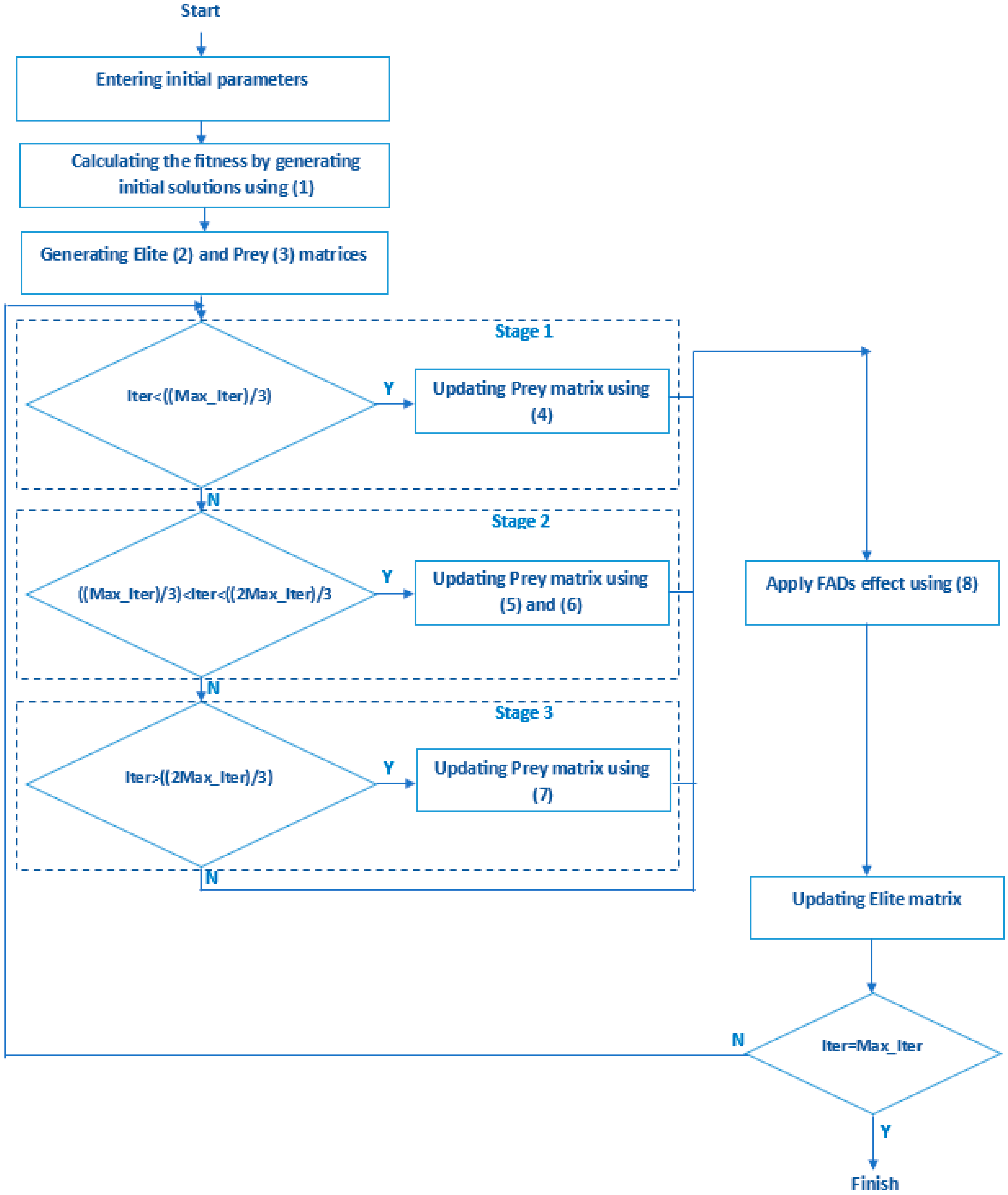
The algorithm is basically structured according to three phases. These phases are scenarios created by considering the speed rate of the prey and the predator. MPA utilizes these three stages to update solutions based on the speed ratio of predator and prey. They are the following:

In stage 1, the predator moves faster than the prey. It is used in the initial iterations of optimization where discovery is important. The best strategy for the predator is to not move at all in this phase. If Iter < ((Max_Iter)/3), this phase occurs. Iter is the current iteration number. Max_Iter is the maximum iteration number. The mathematical equation for this stage is presented below. $R_B$ is a vector containing random numbers based on normal distribution representing the Brownian motion. P is a constant number, and its value is 0.5. R represents a random number in the range [0, 1]. The multiplication of $R_B$ by prey simulates the movement of prey.

$$\begin{gathered} {\overrightarrow{stepsize}}_i={\overrightarrow{R}}_B\otimes \left({\overrightarrow{Elite}}_i-{\overrightarrow{R}}_B\otimes {\overrightarrow{Prey}}_i\right) i=1, . . . n \\ {\overrightarrow{Prey}}_i={\overrightarrow{Prey}}_i+P·\overrightarrow{R}\otimes {\overrightarrow{stepsize}}_i \end{gathered}$$

(4)

In stage 2, the predator and the prey move at the same speed. Half of the population is reserved for exploration and half for exploitation. The predator is responsible for reconnaissance, and the prey is responsible for exploitation. If the prey moves in Lévy, the predator must move in Brownian. If ((Max_Iter)/3) < Iter < ((2Max_Iter)/3, this phase occurs. For the first half of the population, that is, for the prey that used the Lévy motion, (5) is used. For the other half of the population, namely, the predator performing the Brownian motion, (6) is used.

$$\begin{gathered} {\overrightarrow{stepsize}}_i={\overrightarrow{R}}_L\otimes \left({\overrightarrow{Elite}}_i-{\overrightarrow{R}}_L\otimes {\overrightarrow{Prey}}_i\right) i=1, . . . n/2 \\ {\overrightarrow{Prey}}_i={\overrightarrow{Prey}}_i+P·\overrightarrow{R}\otimes {\overrightarrow{stepsize}}_i \end{gathered}$$

(5)

$$\begin{gathered} {\overrightarrow{stepsize}}_i={\overrightarrow{R}}_B\otimes \left({\overrightarrow{R}}_B\otimes {\overrightarrow{Elite}}_i-{\overrightarrow{Prey}}_i\right) i=n/2, . . . n \\ {\overrightarrow{Prey}}_i={\overrightarrow{Elite}}_i+P·CF\otimes {\overrightarrow{stepsize}}_i \\ CF={\left(1-\frac{Iter}{Max\_Iter}\right)}^{\left(2\frac{Iter}{Max\_Iter}\right)} \end{gathered}$$

(6)

In stage 3, the predator moves faster than the prey. The best strategy for the predator is Lévy in this stage. If Iter > ((2Max_Iter)/3), this phase occurs. The mathematical equation for this stage is presented below:

$$\begin{gathered} {\overrightarrow{stepsize}}_i={\overrightarrow{R}}_L\otimes \left({\overrightarrow{R}}_L\otimes {\overrightarrow{Elite}}_i-{\overrightarrow{Prey}}_i\right) i=1, . . . n \\ {\overrightarrow{Prey}}_i={\overrightarrow{Elite}}_i+P·CF\otimes {\overrightarrow{stepsize}}_i \end{gathered}$$

(7)

The behavior of the marine predators can be affected by the factors such as eddy formation or Fish Aggregating Devices (FADs). The effect of FADs is formulated as follows. Here, FADs is 0.2. $\overrightarrow{U}$ is the binary vector with arrays including zero and one. r is the uniform random number in [0, 1]. ${\overrightarrow{X}}_{min}$ and ${\overrightarrow{X}}_{max}$ are the vectors containing the lower and upper bounds of the dimensions. r1 and r2 denote random indexes of the prey matrix.

$${\overrightarrow{Prey}}_i=\left\{\begin{array}{c}{\overrightarrow{Prey}}_i+CF\left[{\overrightarrow{X}}_{min}+\overrightarrow{R} \otimes \left({\overrightarrow{X}}_{max}-{\overrightarrow{X}}_{min}\right)\right]\otimes \overrightarrow{U}, r\le FADs\hfill \\ {\overrightarrow{Prey}}_i+\left[FADs\left(1-r\right)+r\right]\left({\overrightarrow{Prey}}_{r1}-{\overrightarrow{Prey}}_{r2}\right), r>FADs\hfill \end{array}\right.$$

(8)

Marine predators have good memories. They remember places where they successfully hunted for foraging. This situation is simulated as a memory saving in MPA. After the prey is updated and the FADs effect is applied, the results are evaluated. Elite is updated if the results have better value. Thus, the solution quality increases. A flowchart showing the process in MPA is given in Figure 1.

3.2. Feed-Forward Neural Network (FFNN)

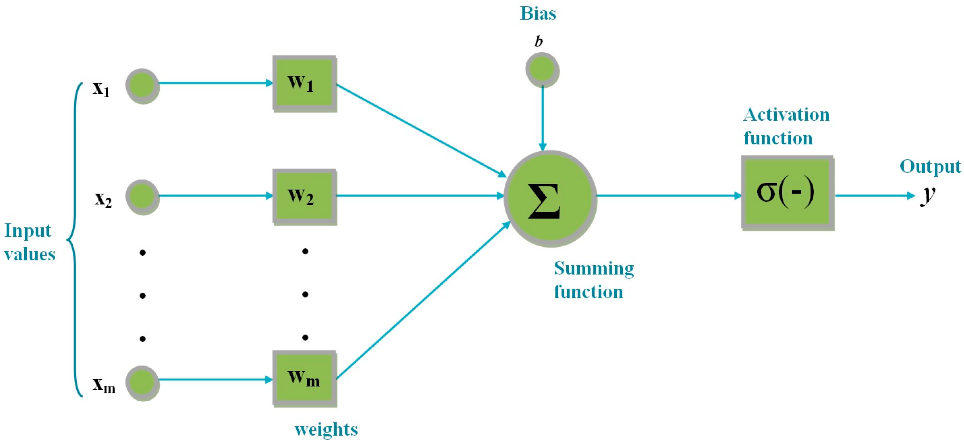
A FFNN generally consists of input, hidden, and output layers. It is formed by the interconnection of many neurons. Information transfer is from the input layer to the output layer. As seen in (9), calculations are performed on artificial neurons in the structure of the network. x is the input value. w represents the weight value. b is the bias value. f is the activation function. y is the output of the artificial neuron. Here, the summing function is used as the transfer function. Each artificial neuron can be the input of a different artificial neuron. There is no interaction between artificial neurons in the same layer. The general structure of artificial neurons is shown in Figure 2. Weight and bias values in FFNN directly affect the success of the network. It is aimed at finding the most appropriate weight and bias values in the training of the network. Two data sets have an important place in the network training process. These are training and test datasets. The training dataset is used during the training of the network. The training process is guided according to the error value obtained during the training. The error value is calculated from the relationship between the actual output and the predicted output. In successful training, the error value should be low. The training process of FFNN takes place over the data known. In the test process, data that has not been known before are given to the network. It is expected that a successful network will also be effective in the testing process.

$$y=f\left(\sum _{i=1}^m{w}_i{x}_i+b\right)$$

(9)

4. Simulation Results

In this study, the training of FFNN was realized by using MPA for the identification of nonlinear systems. The nonlinear systems given in

Table 1. Nonlinear systems used in applications.

System	Equation	Inputs	Output	Number of Training/Test Data
D1	$y\left(k+1\right)=\frac{y\left(k\right)y\left(k-1\right)\left[y\left(k\right)+2.5\right]}{1+{\left[y\left(k\right)\right]}^2+{\left[y\left(k-1\right)\right]}^2}+u\left(k\right)$ $u\left(k\right)=\sin \left(2\pi k/25\right)$	$y\left(k\right),y\left(k-1\right), u\left(k\right)$	$y\left(k+1\right)$	200/50
D2	$y\left(k+1\right)=\frac{y\left(k\right)}{1+y\left(k-1\right)}+{u\left(k\right)}^3$ $u\left(k\right)=\sin \left(\pi k/25\right)$	$y\left(k\right),y\left(k-1\right), u\left(k\right)$	$y\left(k+1\right)$	200/50
S1	$y=2\sin \left(\pi x_1\right)$	x1	y	80/20
S2	$y=10.391\left\{\left(x_1-0.4\right)\left(x_2-0.6\right)+0.36\right\}$	x1, x2	y	80/20
S3	$y=\tanh \left(x_1+x_2-11\right)$	x1, x2	y	80/20
S4	$y=1+{x_1}^{0.5}+{x_2}^{-1}+{x_3}^{-1.5}$	x1, x2, x3	y	173/43

were used for the applications. As seen in Table 1, D1 and D2 are in a dynamic structure. Other systems are nonlinear systems with static behavior. D1, D2, and S4 consist of three inputs. S1 has one input. Other systems consist of two inputs. All systems have one output. In the identification of all systems, 80% of the data is reserved for the training process. The rest belongs to the testing process.

Different network structures are used to analyze the effect of network structure on performance in applications. For each system, neurons in the range of [2,15] were utilized in the hidden layer, and the results were obtained. In other words, 14 different network structures were created for each system, and their effects on performance were evaluated. The sigmoid function was used for each neuron. At the same time, bias was applied. All data for the training and testing process are scaled in the [0, 1] range. All the results in this study were obtained by considering the scaled data. The number of search agents and the maximum number of iterations of MPA were taken as 20 and 2500, respectively. Mean squared error (MSE) was used as the error metric. Each application was run 30 times, and the mean error value was calculated.

The training results obtained for D1 are given in

Table 2. Training results obtained with the proposed approach for the D1 system.

System	Network Structure	The Results
		Best	Mean	Worst	Std.
D1	3-2-1	3.4 × 10−4	6.6 × 10−4	8.3 × 10−4	1.5 × 10−4
	3-3-1	2.1 × 10−4	4.2 × 10−4	6.5 × 10−4	1.5 × 10−4
	3-4-1	1.4 × 10−4	3.3 × 10−4	8.2 × 10−4	1.5 × 10−4
	3-5-1	1.5 × 10−4	3.4 × 10−4	6.0 × 10−4	1.3 × 10−4
	3-6-1	1.3 × 10−4	2.8 × 10−4	5.6 × 10−4	1.1 × 10−4
	3-7-1	1.1 × 10−4	2.4 × 10−4	4.2 × 10−4	9.0 × 10−5
	3-8-1	8.9 × 10−5	2.4 × 10−4	4.9 × 10−4	9.3 × 10−5
	3-9-1	1.2 × 10−4	2.5 × 10−4	5.9 × 10−4	1.1 × 10−4
	3-10-1	1.2 × 10−4	2.8 × 10−4	5.8 × 10−4	1.2 × 10−4
	3-11-1	9.4 × 10−5	2.7 × 10−4	5.0 × 10−4	9.3 × 10−5
	3-12-1	9.4 × 10−5	2.3 × 10−4	5.4 × 10−4	8.7 × 10−5
	3-13-1	1.1 × 10−4	2.4 × 10−4	4.7 × 10−4	9.1 × 10−5
	3-14-1	9.1 × 10−5	2.4 × 10−4	4.4 × 10−4	8.4 × 10−5
	3-15-1	1.1 × 10−4	2.4 × 10−4	3.9 × 10−4	8.1 × 10−5

. The best error value was found with a 3-8-1 network structure. The best mean error value was obtained as 2.3 × 10⁻⁴ with 3-12-1. With 3-12-1, a performance increase of approximately 66% was achieved compared to 3-2-1. The test results of D1 are presented in

Table 3. Test results obtained with the proposed approach for the D1 system.

System	Network Structure	The Results
		Best	Mean	Worst	Std.
D1	3-2-1	3.4 × 10−4	7.5 × 10−4	1.3 × 10−3	1.8 × 10−4
	3-3-1	2.1 × 10−4	4.9 × 10−4	8.7 × 10−4	2.0 × 10−4
	3-4-1	1.5 × 10−4	4.3 × 10−4	8.7 × 10−4	1.7 × 10−4
	3-5-1	1.5 × 10−4	4.2 × 10−4	1.2 × 10−3	2.1 × 10−4
	3-6-1	1.3 × 10−4	3.1 × 10−4	6.3 × 10−4	1.3 × 10−4
	3-7-1	1.1 × 10−4	2.7 × 10−4	5.3 × 10−4	1.1 × 10−4
	3-8-1	7.9 × 10−5	2.5 × 10−4	5.1 × 10−4	1.1 × 10−4
	3-9-1	1.5 × 10−4	3.3 × 10−4	9.8 × 10−4	1.7 × 10−4
	3-10-1	1.1 × 10−4	3.1 × 10−4	6.4 × 10−4	1.4 × 10−4
	3-11-1	9.5 × 10−5	2.7 × 10−4	7.0 × 10−4	1.1 × 10−4
	3-12-1	9.8 × 10−5	2.3 × 10−4	5.3 × 10−4	8.7 × 10−5
	3-13-1	7.8 × 10−5	2.6 × 10−4	4.9 × 10−4	1.0 × 10−4
	3-14-1	9.6 × 10−5	2.6 × 10−4	4.6 × 10−4	9.0 × 10−5
	3-15-1	1.0 × 10−4	2.4 × 10−4	3.4 × 10−4	7.1 × 10−5

. As in the training results, the mean best error value was found with the 3-12-1 network structure. Compared to the 3-2-1 network structure, a significant performance increase was achieved. The best test error value was obtained as 7.8 × 10⁻⁵ with a 3-13-1 network structure. Effective standard deviation values were achieved in both the training and testing processes.

The training results of D2 are presented in

Table 4. Training results obtained with the proposed approach for the D2 system.

System	Network Structure	The Results
		Best	Mean	Worst	Std.
D2	3-2-1	3.8 × 10−3	3.9 × 10−3	4.3 × 10−3	1.5 × 10−4
	3-3-1	2.4 × 10−3	2.9 × 10−3	3.8 × 10−3	4.1 × 10−4
	3-4-1	1.6 × 10−3	2.5 × 10−3	4.0 × 10−3	4.8 × 10−4
	3-5-1	1.7 × 10−3	2.2 × 10−3	3.1 × 10−3	3.5 × 10−4
	3-6-1	1.7 × 10−3	2.2 × 10−3	3.1 × 10−3	3.4 × 10−4
	3-7-1	1.6 × 10−3	2.1 × 10−3	2.9 × 10−3	3.7 × 10−4
	3-8-1	1.4 × 10−3	2.1 × 10−3	3.2 × 10−3	5.1 × 10−4
	3-9-1	1.5 × 10−3	2.1 × 10−3	3.0 × 10−3	4.2 × 10−4
	3-10-1	1.4 × 10−3	2.0 × 10−3	3.3 × 10−3	4.6 × 10−4
	3-11-1	1.4 × 10−3	2.0 × 10−3	2.8 × 10−3	4.0 × 10−4
	3-12-1	1.1 × 10−3	1.8 × 10−3	2.4 × 10−3	3.2 × 10−4
	3-13-1	1.3 × 10−3	1.9 × 10−3	3.1 × 10−3	4.5 × 10−4
	3-14-1	1.4 × 10−3	1.9 × 10−3	3.1 × 10−3	4.4 × 10−4
	3-15-1	1.3 × 10−3	1.8 × 10−3	2.7 × 10−3	3.4 × 10−4

. The best error value was obtained by using a 3-12-1 network structure. The best error value is 1.1 × 10⁻³. When the mean error values were examined, the best mean error value was found with a 3-15-1 network structure. The performance usually increases until the number of neurons is 15 in the hidden layer. The test results obtained for D2 are given in

Table 5. Test results obtained with the proposed approach for the D2 system.

System	Network Structure	The Results
		Best	Mean	Worst	Std.
D2	3-2-1	3.8 × 10−3	4.0 × 10−3	4.8 × 10−3	2.8 × 10−4
	3-3-1	2.5 × 10−3	3.0 × 10−3	4.0 × 10−3	4.1 × 10−4
	3-4-1	1.6 × 10−3	2.6 × 10−3	4.0 × 10−3	5.0 × 10−4
	3-5-1	1.7 × 10−3	2.4 × 10−3	3.2 × 10−3	3.7 × 10−4
	3-6-1	1.7 × 10−3	2.3 × 10−3	3.7 × 10−3	4.0 × 10−4
	3-7-1	1.6 × 10−3	2.2 × 10−3	3.0 × 10−3	3.9 × 10−4
	3-8-1	1.4 × 10−3	2.2 × 10−3	3.5 × 10−3	5.2 × 10−4
	3-9-1	1.5 × 10−3	2.2 × 10−3	3.7 × 10−3	5.0 × 10−4
	3-10-1	1.5 × 10−3	2.1 × 10−3	3.4 × 10−3	5.0 × 10−4
	3-11-1	1.4 × 10−3	2.0 × 10−3	3.0 × 10−3	4.2 × 10−4
	3-12-1	1.2 × 10−3	1.9 × 10−3	2.6 × 10−3	3.4 × 10−4
	3-13-1	1.3 × 10−3	2.0 × 10−3	3.3 × 10−3	5.0 × 10−4
	3-14-1	1.4 × 10−3	2.0 × 10−3	3.1 × 10−3	4.7 × 10−4
	3-15-1	1.3 × 10−3	1.8 × 10−3	2.9 × 10−3	3.6 × 10−4

. As in the training results, the best error value was found with a 3-12-1 network structure, while the best mean error value was obtained with a 3-15-1 network structure.

The training results that obtained for S1 are given in

Table 6. Training results obtained with the proposed approach for the S1 system.

System	Network Structure	The Results
		Best	Mean	Worst	Std.
S1	1-2-1	1.2 × 10−3	1.6 × 10−3	2.4 × 10−3	4.9 × 10−4
	1-3-1	6.0 × 10−4	7.0 × 10−4	9.2 × 10−4	7.9 × 10−5
	1-4-1	5.0 × 10−5	4.2 × 10−4	1.2 × 10−3	3.1 × 10−4
	1-5-1	5.5 × 10−5	3.7 × 10−4	6.8 × 10−4	2.3 × 10−4
	1-6-1	5.1 × 10−5	3.0 × 10−4	8.4 × 10−4	2.6 × 10−4
	1-7-1	4.9 × 10−5	1.4 × 10−4	6.7 × 10−4	1.3 × 10−4
	1-8-1	5.6 × 10−5	2.2 × 10−4	6.2 × 10−4	1.8 × 10−4
	1-9-1	4.7 × 10−5	1.8 × 10−4	6.5 × 10−4	1.7 × 10−4
	1-10-1	5.3 × 10−5	1.4 × 10−4	5.8 × 10−4	1.4 × 10−4
	1-11-1	4.6 × 10−5	1.4 × 10−4	5.4 × 10−4	1.2 × 10−4
	1-12-1	5.3 × 10−5	1.0 × 10−4	4.1 × 10−4	6.4 × 10−5
	1-13-1	4.7 × 10−5	1.5 × 10−4	5.0 × 10−4	1.2 × 10−4
	1-14-1	5.8 × 10−5	1.4 × 10−4	4.0 × 10−4	8.2 × 10−5
	1-15-1	4.7 × 10−5	1.4 × 10−4	3.9 × 10−4	8.4 × 10−5

. The best error value was found as 4.6 × 10⁻⁵ with a 1-11-1 network structure. A serious performance increase was observed until the number of neurons was 11 in the hidden layer. The best mean error value was obtained with a 1-12-1 network structure. The test results of S1 are presented in

Table 7. Test results obtained with the proposed approach for the S1 system.

System	Network Structure	The Results
		Best	Mean	Worst	Std.
S1	1-2-1	2.4 × 10−3	2.9 × 10−3	4.4 × 10−3	7.9 × 10−4
	1-3-1	1.3 × 10−3	1.8 × 10−3	2.4 × 10−3	3.8 × 10−4
	1-4-1	4.3 × 10−4	1.4 × 10−3	2.4 × 10−3	6.3 × 10−4
	1-5-1	4.3 × 10−4	1.3 × 10−3	2.4 × 10−3	5.6 × 10−4
	1-6-1	3.3 × 10−4	1.1 × 10−3	2.3 × 10−3	5.9 × 10−4
	1-7-1	3.4 × 10−4	8.8 × 10−4	1.9 × 10−3	3.6 × 10−4
	1-8-1	3.4 × 10−4	8.2 × 10−4	1.9 × 10−3	3.9 × 10−4
	1-9-1	3.7 × 10−4	9.8 × 10−4	2.4 × 10−3	5.4 × 10−4
	1-10-1	3.8 × 10−4	9.0 × 10−4	1.5 × 10−3	3.0 × 10−4
	1-11-1	3.0 × 10−4	1.0 × 10−3	3.5 × 10−3	5.7 × 10−4
	1-12-1	3.2 × 10−4	9.7 × 10−4	1.9 × 10−3	4.0 × 10−4
	1-13-1	4.1 × 10−4	1.1 × 10−3	2.9 × 10−3	4.9 × 10−4
	1-14-1	3.5 × 10−4	9.8 × 10−4	1.9 × 10−3	4.6 × 10−4
	1-15-1	4.6 × 10−4	1.0 × 10−3	2.7 × 10−3	5.2 × 10−4

. As in the training results, the best test error value was reached with a 1-11-1 network structure. The best mean error value was found as 8.2 × 10⁻⁴ with a 1-8-1 network structure. In the training results, the most effective standard deviation value was obtained with a 1-12-1 network structure. In the test results, the best standard deviation value was found in the 1-10-1 network structure.

The training results of S2 are presented in

Table 8. Training results obtained with the proposed approach for the S2 system.

System	Network Structure	The Results
		Best	Mean	Worst	Std.
S2	2-2-1	4.4 × 10−3	5.0 × 10−3	6.0 × 10−3	3.4 × 10−4
	2-3-1	6.6 × 10−4	9.1 × 10−4	2.8 × 10−3	4.9 × 10−4
	2-4-1	1.4 × 10−4	3.8 × 10−4	7.4 × 10−4	2.0 × 10−4
	2-5-1	5.5 × 10−5	2.2 × 10−4	6.0 × 10−4	1.4 × 10−4
	2-6-1	5.5 × 10−5	1.4 × 10−4	3.5 × 10−4	6.0 × 10−5
	2-7-1	5.0 × 10−5	1.3 × 10−4	2.5 × 10−4	5.0 × 10−5
	2-8-1	5.0 × 10−5	1.4 × 10−4	7.0 × 10−4	1.1 × 10−4
	2-9-1	4.7 × 10−5	1.1 × 10−4	2.8 × 10−4	6.9 × 10−5
	2-10-1	4.9 × 10−5	1.0 × 10−4	2.7 × 10−4	4.6 × 10−5
	2-11-1	6.4 × 10−5	1.1 × 10−4	2.0 × 10−4	3.7 × 10−5
	2-12-1	4.4 × 10−5	1.2 × 10−4	4.9 × 10−4	8.2 × 10−5
	2-13-1	6.1 × 10−5	1.2 × 10−4	2.2 × 10−4	4.0 × 10−5
	2-14-1	5.7 × 10−5	1.1 × 10−4	2.7 × 10−4	4.5 × 10−5
	2-15-1	5.2 × 10−5	1.1 × 10−4	2.6 × 10−4	5.0 × 10−5

. The best error value was found with a 2-12-1 network structure. A significant increase in performance was observed until reaching the 2-12-1 network structure from the 2-12-1 network structure. The best mean error value was found with a 2-10-1 network structure as 1.0 × 10⁻⁴. The test results obtained for S2 are given in

Table 9. Test results obtained with the proposed approach for the S2 system.

System	Network Structure	The Results
		Best	Mean	Worst	Std.
S2	2-2-1	9.2 × 10−3	1.5 × 10−2	2.5 × 10−2	6.1 × 10−3
	2-3-1	5.4 × 10−3	7.0 × 10−3	2.5 × 10−2	3.4 × 10−3
	2-4-1	7.1 × 10−4	3.8 × 10−3	8.4 × 10−3	2.4 × 10−3
	2-5-1	6.7 × 10−4	3.2 × 10−3	1.0 × 10−2	2.2 × 10−3
	2-6-1	1.0 × 10−3	2.3 × 10−3	8.5 × 10−3	1.3 × 10−3
	2-7-1	8.0 × 10−4	2.4 × 10−3	8.8 × 10−3	1.6 × 10−3
	2-8-1	1.1 × 10−3	2.7 × 10−3	1.5 × 10−2	2.5 × 10−3
	2-9-1	1.3 × 10−3	2.7 × 10−3	9.2 × 10−3	1.7 × 10−3
	2-10-1	7.5 × 10−4	2.4 × 10−3	6.5 × 10−3	1.0 × 10−3
	2-11-1	7.8 × 10−4	2.4 × 10−3	6.0 × 10−3	1.1 × 10−3
	2-12-1	1.4 × 10−3	2.6 × 10−3	5.0 × 10−3	9.1 × 10−4
	2-13-1	1.3 × 10−3	2.8 × 10−3	8.3 × 10−3	1.2 × 10−3
	2-14-1	1.0 × 10−3	3.1 × 10−3	7.3 × 10−3	1.4 × 10−3
	2-15-1	1.5 × 10−3	3.3 × 10−3	9.3 × 10−3	1.9 × 10−3

. The best test error value was reached with a 2-5-1 network structure. The best mean error value was obtained with the 2-6-1 network structure. It is seen that the standard deviation values obtained from the training and error results are effective.

The training results that found for S3 are given in

Table 10. Training results obtained with the proposed approach for the S3 system.

System	Network Structure	The Results
		Best	Mean	Worst	Std.
S3	2-2-1	3.0 × 10−5	3.1 × 10−5	3.2 × 10−5	6.0 × 10−7
	2-3-1	8.2 × 10−6	1.6 × 10−5	3.2 × 10−5	7.2 × 10−6
	2-4-1	8.0 × 10−6	1.6 × 10−5	3.4 × 10−5	6.2 × 10−6
	2-5-1	7.1 × 10−6	1.3 × 10−5	2.9 × 10−5	4.9 × 10−6
	2-6-1	7.5 × 10−6	1.5 × 10−5	3.1 × 10−5	5.3 × 10−6
	2-7-1	6.7 × 10−6	1.6 × 10−5	4.0 × 10−5	8.4 × 10−6
	2-8-1	6.1 × 10−6	1.4 × 10−5	2.9 × 10−5	5.6 × 10−6
	2-9-1	5.3 × 10−6	1.4 × 10−5	2.9 × 10−5	5.2 × 10−6
	2-10-1	6.1 × 10−6	1.4 × 10−5	2.7 × 10−5	5.4 × 10−6
	2-11-1	6.0 × 10−6	1.7 × 10−5	1.1 × 10−4	1.8 × 10−5
	2-12-1	6.2 × 10−6	1.4 × 10−5	4.2 × 10−5	6.5 × 10−6
	2-13-1	7.9 × 10−6	1.8 × 10−5	4.6 × 10−5	1.0 × 10−5
	2-14-1	6.8 × 10−6	1.5 × 10−5	2.9 × 10−5	5.2 × 10−6
	2-15-1	7.2 × 10−6	1.2 × 10−5	2.4 × 10−5	3.8 × 10−6

. The best error value was reached with a 2-9-1 network structure. It is 5.3 × 10⁻⁶. The best mean error value was found with a 2-15-1 network structure. In

Table 11. Test results obtained with the proposed approach for the S3 system.

System	Network Structure	The Results
		Best	Mean	Worst	Std.
S3	2-2-1	1.7 × 10−3	1.7 × 10−3	1.8 × 10−3	1.9 × 10−5
	2-3-1	1.5 × 10−3	1.6 × 10−3	1.9 × 10−3	1.1 × 10−4
	2-4-1	1.1 × 10−3	1.5 × 10−3	2.1 × 10−3	2.4 × 10−4
	2-5-1	1.2 × 10−3	1.6 × 10−3	2.2 × 10−3	2.3 × 10−4
	2-6-1	1.2 × 10−3	1.6 × 10−3	2.3 × 10−3	2.5 × 10−4
	2-7-1	1.1 × 10−3	1.6 × 10−3	2.6 × 10−3	3.6 × 10−4
	2-8-1	1.0 × 10−3	1.5 × 10−3	2.1 × 10−3	2.4 × 10−4
	2-9-1	1.1 × 10−3	1.5 × 10−3	2.3 × 10−3	3.0 × 10−4
	2-10-1	9.7 × 10−4	1.5 × 10−3	2.0 × 10−3	2.5 × 10−4
	2-11-1	1.1 × 10−3	1.7 × 10−3	5.2 × 10−3	7.1 × 10−4
	2-12-1	8.0 × 10−4	1.4 × 10−3	2.0 × 10−3	2.9 × 10−4
	2-13-1	8.7 × 10−4	1.6 × 10−3	3.3 × 10−3	5.2 × 10−4
	2-14-1	9.9 × 10−4	1.6 × 10−3	3.6 × 10−3	5.4 × 10−4
	2-15-1	1.2 × 10−3	1.5 × 10−3	2.3 × 10−3	2.4 × 10−4

, the test results of S3 are presented. The best test error value and the best mean error value were found with a 2-12-1 network structure. As seen in both the training and test results, the most effective standard deviation value was obtained with a 2-2-1 network structure.

In

Table 12. Training results obtained with the proposed approach for the S4 system.

System	Network Structure	The Results
		Best	Mean	Worst	Std.
S4	3-2-1	2.9 × 10−3	3.0 × 10−3	3.2 × 10−3	1.3 × 10−4
	3-3-1	4.3 × 10−4	5.6 × 10−4	8.9 × 10−4	1.2 × 10−4
	3-4-1	2.5 × 10−4	4.3 × 10−4	6.7 × 10−4	9.4 × 10−5
	3-5-1	2.0 × 10−4	3.7 × 10−4	7.3 × 10−4	1.4 × 10−4
	3-6-1	2.2 × 10−4	3.4 × 10−4	5.2 × 10−4	8.0 × 10−5
	3-7-1	1.6 × 10−4	3.0 × 10−4	5.1 × 10−4	8.0 × 10−5
	3-8-1	1.5 × 10−4	2.9 × 10−4	5.1 × 10−4	8.7 × 10−5
	3-9-1	1.5 × 10−4	3.0 × 10−4	6.0 × 10−4	9.5 × 10−5
	3-10-1	1.4 × 10−4	2.8 × 10−4	4.5 × 10−4	6.9 × 10−5
	3-11-1	1.2 × 10−4	2.5 × 10−4	3.7 × 10−4	6.5 × 10−5
	3-12-1	1.3 × 10−4	2.6 × 10−4	3.8 × 10−4	7.5 × 10−5
	3-13-1	1.3 × 10−4	2.8 × 10−4	4.9 × 10−4	9.5 × 10−5
	3-14-1	1.3 × 10−4	2.7 × 10−4	4.5 × 10−4	8.4 × 10−5
	3-15-1	1.5 × 10−4	2.5 × 10−4	3.9 × 10−4	6.8 × 10−5

, the training results for S4 are presented. An increase was observed in the performance until the number of neurons was nine in the hidden layer. The best standard deviation value was obtained with a 3-11-1 network structure. The test results of S4 are given in

Table 13. Test results obtained with the proposed approach for the S4 system.

System	Network Structure	The Results
		Best	Mean	Worst	Std.
S4	3-2-1	3.6 × 10−3	4.0 × 10−3	4.5 × 10−3	4.4 × 10−4
	3-3-1	6.4 × 10−4	1.1 × 10−3	2.0 × 10−3	3.7 × 10−4
	3-4-1	4.0 × 10−4	1.0 × 10−3	1.8 × 10−3	3.8 × 10−4
	3-5-1	4.3 × 10−4	8.6 × 10−4	1.5 × 10−3	2.7 × 10−4
	3-6-1	3.8 × 10−4	9.4 × 10−4	1.7 × 10−3	3.2 × 10−4
	3-7-1	3.5 × 10−4	7.8 × 10−4	1.8 × 10−3	3.2 × 10−4
	3-8-1	4.6 × 10−4	8.8 × 10−4	1.5 × 10−3	3.1 × 10−4
	3-9-1	2.8 × 10−4	9.3 × 10−4	2.1 × 10−3	4.1 × 10−4
	3-10-1	3.2 × 10−4	8.9 × 10−4	1.4 × 10−3	2.6 × 10−4
	3-11-1	2.5 × 10−4	8.7 × 10−4	1.5 × 10−3	3.4 × 10−4
	3-12-1	3.6 × 10−4	8.6 × 10−4	1.7 × 10−3	3.2 × 10−4
	3-13-1	2.5 × 10−4	8.5 × 10−4	1.5 × 10−3	3.4 × 10−4
	3-14-1	2.8 × 10−4	9.7 × 10−4	1.6 × 10−3	3.3 × 10−4
	3-15-1	3.1 × 10−4	8.8 × 10−4	1.5 × 10−3	2.8 × 10−4

. The best error value was reached with the 3-11-1 network structure. With a 3-7-1 network structure, the best mean error value was found as 7.8 × 10⁻⁴. A 3-10-1 network structure has the best standard deviation value in the test.

It is important to compare the real output and the predicted output in order to analyze the success status of the training process. In Figure 3, the comparison of the real output and the predicted output is shown for all systems. These graphs were created by taking into account the best results. In the graphs of D1, S1, S2, S3, and S4, it is seen that the real and the predicted outputs overlap exactly. In D2, the similarity rate of both outputs is very high. This is an indication of the success of the training process for the relevant systems.

The performance of MPA in solving related problems was compared with different metaheuristic algorithms. The results of other algorithms are taken from [12]. The population size and the maximum number of iterations taken were the same for a fair comparison. For each system in the training process of ANN with MPA, neurons between 2 and 15 were utilized in the hidden layer, and the results were obtained. However, in [12], the performance of networks with only 5, 10, and 15 neurons in the hidden layer was examined. For a fair comparison, the results of networks with 5, 10, and 15 neurons were also taken into account in MPA and placed in the comparison tables. The algorithms used in the comparison are ABC, BAT, CS, FPA, PSO, JAYA, TLBO, SCA, BBO, WOA, BSA, HS, BA, MVO, MFO, and SSA.

The comparison of the results obtained for D1 is given in

Table 14. Comparison of the best mean error values obtained using different metaheuristic algorithms for D1 [12].

Algorithm	Train		Test
	Network Structure	Mean (MSE)	Network Structure	Mean (MSE)
ABC	3-15-1	5.3 × 10−4	3-15-1	6.6 × 10−4
BAT	3-15-1	5.2 × 10−3	3-15-1	5.3 × 10−3
CS	3-10-1	8.6 × 10−4	3-5-1	9.3 × 10−4
FPA	3-10-1	9.9 × 10−4	3-10-1	1.1 × 10−3
PSO	3-5-1	1.3 × 10−3	3-5-1	1.3 × 10−3
JAYA	3-5-1	1.3 × 10−2	3-5-1	1.3 × 10−2
TLBO	3-10-1	6.2 × 10−4	3-10-1	6.7 × 10−4
SCA	3-5-1	3.5 × 10−3	3-5-1	3.9 × 10−3
BBO	3-5-1	5.2 × 10−4	3-5-1	6.1 × 10−4
WOA	3-5-1	5.3 × 10−3	3-5-1	5.7 × 10−3
BSA	3-15-1	6.5 × 10−3	3-15-1	6.8 × 10−3
HS	3-5-1	5.7 × 10−3	3-5-1	5.8 × 10−3
BA	3-10-1	6.7 × 10−3	3-10-1	7.0 × 10−3
MVO	3-15-1	6.7 × 10−4	3-15-1	7.6 × 10−4
MFO	3-15-1	5.4 × 10−4	3-15-1	6.3 × 10−4
SSA	3-15-1	6.9 × 10−4	3-15-1	8.1 × 10−4
Proposed	3-15-1	2.4 × 10−4	3-15-1	2.4 × 10−4

. The best training result was found with the proposed approach as 2.4 × 10⁻⁴. Likewise, the best test error value belongs to the proposed approach, and it is 2.4 × 10⁻⁴. After the proposed approach, the best training and test results were found with BBO. In addition, in seven of the seventeen algorithms, the 3-15-1 network structure was seen to be more effective.

In

Table 15. Comparison of the best mean error values obtained using different metaheuristic algorithms for D2 [12].

Algorithm	Train		Test
	Network Structure	Mean (MSE)	Network Structure	Mean (MSE)
ABC	3-15-1	2.9 × 10−3	3-15-1	3.0 × 10−3
BAT	3-15-1	8.6 × 10−3	3-15-1	9.0 × 10−3
CS	3-15-1	3.4 × 10−3	3-15-1	3.5 × 10−3
FPA	3-15-1	3.7 × 10−3	3-15-1	3.9 × 10−3
PSO	3-5-1	4.1 × 10−3	3-5-1	4.1 × 10−3
JAYA	3-10-1	1.4 × 10−2	3-10-1	1.4 × 10−2
TLBO	3-10-1	3.0 × 10−3	3-10-1	3.2 × 10−3
SCA	3-5-1	6.2 × 10−3	3-5-1	6.6 × 10−3
BBO	3-10-1	2.4 × 10−3	3-10-1	2.5 × 10−3
WOA	3-5-1	8.8 × 10−3	3-5-1	9.1 × 10−3
BSA	3-10-1	1.1 × 10−2	3-10-1	1.1 × 10−2
HS	3-5-1	9.8 × 10−3	3-5-1	9.8 × 10−3
BA	3-10-1	9.7 × 10−3	3-10-1	1.0 × 10−2
MVO	3-15-1	3.1 × 10−3	3-15-1	3.2 × 10−3
MFO	3-15-1	2.4 × 10−3	3-15-1	2.5 × 10−3
SSA	3-15-1	3.6 × 10−3	3-15-1	3.8 × 10−3
Proposed	3-15-1	1.8 × 10−3	3-15-1	1.8 × 10−3

, the comparison of the results belonging to D2 is presented. When the relevant table is examined, it is seen that the best training and test error values are owned by the proposed approach, as in D1. With a 3-15-1 network structure, the training and test error value was found as 1.8 × 10⁻³. MFO and BBO are algorithms with the best training and test error values after the proposed approach. The training and test error values of these algorithms are 2.4 × 10⁻³ and 2.5 × 10⁻³, respectively. MFO was more effective in the 3-15-1 network structure. On the other hand, BBO achieved a more successful result in the 3-10-1 network structure.

The comparison results of S1 are given in

Table 16. Comparison of the best mean error values obtained using different metaheuristic algorithms for S1 [12].

Algorithm	Train		Test
	Network Structure	Mean (MSE)	Network Structure	Mean (MSE)
ABC	1-15-1	7.1 × 10−4	1-15-1	1.5 × 10−3
BAT	1-10-1	2.2 × 10−2	1-10-1	2.3 × 10−2
CS	1-15-1	7.3 × 10−4	1-10-1	1.6 × 10−3
FPA	1-15-1	8.0 × 10−4	1-15-1	1.7 × 10−3
PSO	1-5-1	1.7 × 10−3	1-5-1	1.7 × 10−3
JAYA	1-10-1	1.3 × 10−2	1-15-1	1.4 × 10−2
TLBO	1-10-1	9.7 × 10−4	1-10-1	1.6 × 10−3
SCA	1-5-1	4.5 × 10−3	1-5-1	5.6 × 10−3
BBO	1-15-1	5.3 × 10−4	1-15-1	1.5 × 10−3
WOA	1-10-1	3.8 × 10−3	1-10-1	5.4 × 10−3
BSA	1-10-1	9.2 × 10−3	1-10-1	1.0 × 10−2
HS	1-5-1	1.1 × 10−2	1-5-1	1.2 × 10−2
BA	1-15-1	6.2 × 10−3	1-10-1	7.2 × 10−3
MVO	1-15-1	4.9 × 10−4	1-15-1	1.5 × 10−3
MFO	1-15-1	3.5 × 10−4	1-15-1	1.4 × 10−3
SSA	1-15-1	7.9 × 10−4	1-15-1	1.8 × 10−3
Proposed	1-10-1	1.4 × 10−4	1-10-1	9.0 × 10−4

. The best training and test error values were obtained by using the proposed algorithm. Unlike D1 and D2, the best error values were achieved when the number of neurons was 10 in the hidden layer. After the proposed algorithm, the best result was found with the MFO in both training and test error values. When the results are examined, it is seen that the performance of the proposed algorithm is significantly better than other algorithms.

In

Table 17. Comparison of the best mean error values obtained using different metaheuristic algorithms for S2 [12].

Algorithm	Train		Test
	Network Structure	Mean (MSE)	Network Structure	Mean (MSE)
ABC	2-10-1	5.4 × 10−4	2-10-1	4.1 × 10−3
BAT	2-15-1	8.9 × 10−3	2-15-1	1.7 × 10−2
CS	2-15-1	9.8 × 10−4	2-10-1	4.4 × 10−3
FPA	2-15-1	1.1 × 10−3	2-10-1	5.8 × 10−3
PSO	2-5-1	1.8 × 10−3	2-5-1	1.8 × 10−3
JAYA	2-5-1	1.6 × 10−2	2-5-1	2.8 × 10−2
TLBO	2-10-1	6.2 × 10−4	2-10-1	4.0 × 10−3
SCA	2-5-1	7.5 × 10−3	2-5-1	1.7 × 10−2
BBO	2-15-1	4.7 × 10−4	2-15-1	4.3 × 10−3
WOA	2-5-1	9.1 × 10−3	2-15-1	2.1 × 10−2
BSA	2-10-1	8.6 × 10−3	2-10-1	1.8 × 10−2
HS	2-5-1	4.9 × 10−3	2-5-1	1.2 × 10−2
BA	2-5-1	1.0 × 10−2	2-10-1	2.3 × 10−2
MVO	2-15-1	5.5 × 10−4	2-15-1	3.8 × 10−3
MFO	2-15-1	5.2 × 10−4	2-15-1	3.7 × 10−3
SSA	2-15-1	1.2 × 10−3	2-15-1	6.7 × 10−3
Proposed	2-10-1	1.0 × 10 −4	2-10-1	2.4 × 10−3

, the comparison results of S2 are given. The best training error value was found by utilizing the proposed algorithm. This value was obtained as 1.0 × 10⁻⁴ with a 2-10-1 network structure. The proposed algorithm is followed by BBO with a 2-15-1 network structure. The best test error value was found with PSO by using a 2-5-1 network structure.

The comparison of results for S3 is presented in

Table 18. Comparison of the best mean error values obtained using different metaheuristic algorithms for S3 [12].

Algorithm	Train		Test
	Network Structure	Mean (MSE)	Network Structure	Mean (MSE)
ABC	2-10-1	2.3 × 10−4	2-5-1	3.4 × 10−3
BAT	2-15-1	1.6 × 10−3	2-15-1	9.2 × 10−3
CS	2-5-1	1.4 × 10−4	2-5-1	3.5 × 10−3
FPA	2-5-1	2.0 × 10−4	2-5-1	4.0 × 10−3
PSO	2-5-1	2.1 × 10−4	2-5-1	2.1 × 10−4
JAYA	2-5-1	6.2 × 10−3	2-5-1	2.4 × 10−2
TLBO	2-5-1	5.6 × 10−5	2-10-1	2.8 × 10−3
SCA	2-5-1	1.2 × 10−3	2-5-1	7.6 × 10−3
BBO	2-10-1	1.0 × 10−4	2-10-1	3.5 × 10−3
WOA	2-5-1	1.6 × 10−3	2-5-1	9.8 × 10−3
BSA	2-15-1	2.2 × 10−3	2-15-1	1.4 × 10−2
HS	2-5-1	2.2 × 10−3	2-5-1	1.0 × 10−2
BA	2-5-1	2.7 × 10−3	2-5-1	9.8 × 10−3
MVO	2-10-1	1.2 × 10−4	2-15-1	3.6 × 10−3
MFO	2-10-1	2.0 × 10−4	2-10-1	4.5 × 10−3
SSA	2-15-1	1.1 × 10−4	2-15-1	3.6 × 10−3
Proposed	2-15-1	1.2 × 10−5	2-15-1	1.5 × 10−3

. The best error value was found with the proposed approach in the 2-15-1 network structure, and it is 1.2 × 10⁻⁵. This value is followed by TLBO with a 2-5-1 network structure. It is seen that the results found with the proposed algorithm in the training error values are much more successful than the results found with other algorithms. The best test error value was found in the PSO with a 2-5-1 network structure. This value is followed by the proposed approach with a 2-15-1 network structure. In both the training and test results, it was observed that the nine algorithms were more effective with the 2-5-1 network structure.

In

Table 19. Comparison of the best mean error values obtained using different metaheuristic algorithms for S4 [12].

Algorithm	Train		Test
	Network Structure	Mean (MSE)	Network Structure	Mean (MSE)
ABC	3-10-1	1.5 × 10−3	3-10-1	2.1 × 10−3
BAT	3-5-1	1.5 × 10−2	3-5-1	1.5 × 10−2
CS	3-10-1	2.5 × 10−3	3-5-1	2.9 × 10−3
FPA	3-5-1	3.1 × 10−3	3-15-1	3.4 × 10−3
PSO	3-5-1	2.1 × 10−3	3-5-1	2.1 × 10−3
JAYA	3-5-1	3.0 × 10−2	3-5-1	2.9 × 10−2
TLBO	3-10-1	4.8 × 10−4	3-10-1	9.7 × 10−4
SCA	3-5-1	7.5 × 10−3	3-5-1	7.6 × 10−3
BBO	3-10-1	8.1 × 10−4	3-5-1	1.4 × 10−3
WOA	3-5-1	8.2 × 10−3	3-5-1	8.2 × 10−3
BSA	3-15-1	1.4 × 10−2	3-15-1	1.4 × 10−2
HS	3-5-1	8.2 × 10−3	3-5-1	7.9 × 10−3
BA	3-5-1	1.7 × 10−2	3-5-1	1.7 × 10−2
MVO	3-15-1	2.0 × 10−3	3-15-1	2.5 × 10−3
MFO	3-15-1	2.2 × 10−3	3-15-1	3.4 × 10−3
SSA	3-15-1	1.7 × 10−3	3-15-1	2.2 × 10−3
Proposed	3-15-1	2.5 × 10 −4	3-5-1	8.6 × 10−4

, the comparison of results for S4 is given. The best training and test error values were obtained with the proposed approach. While the best training result was achieved with the 3-15-1 network structure, the best test error value was achieved with the 3-5-1 network structure. The proposed algorithm is followed by TLBO with a 3-10-1 network structure in training and test error values.

5. Discussion

One of the important problems used to evaluate the performances of approaches based on neural networks and neuro-fuzzy is the identification of nonlinear systems. In this context, there are nonlinear test functions used in the literature. Nonlinear systems can exhibit static or dynamic behaviors due to their structure. There are differences in the behavior of both problem groups. These problems are in the difficult problem group by their nature. Therefore, the success of the developed artificial intelligence approaches to these problem types gives an idea about the success and effectiveness of the related algorithm. For this reason, both static and dynamic nonlinear test problems were used in this study.

The effectiveness of ANN in the modeling of a system is directly related to the training process. Namely, a successful training algorithm is required. Therefore, in this study, MPA was chosen for an effective training process. In the solution of a system, the network structure of the artificial neural network affects the performance positively or negatively. Detailed analysis of the network structure is required for each problem. Therefore, in this study, different network structures were used to solve each problem. Network structures with 2 to 15 neurons in the hidden layer were tested for each problem. In general, it was observed that the performance was worse at a lower number of neurons. Although it varies according to the type of problem, increasing the number of neurons up to a certain level improved the performance. The best mean results obtained for each problem are given in

Table 20. The best mean error values obtained for the systems.

System	Train		Test
	Network Structure	Mean (MSE)	Network Structure	Mean (MSE)
D1	3-12-1	2.3 × 10−4	3-12-1	2.3 × 10−4
D2	3-15-1	1.8 × 10−3	3-15-1	1.8 × 10−3
S1	1-12-1	1.0 × 10−4	1-8-1	8.2 × 10−4
S2	2-10-1	1.0 × 10−4	2-6-1	2.3 × 10−3
S3	2-15-1	1.2 × 10−5	2-12-1	1.4 × 10−3
S4	3-11-1	2.5 × 10−4	3-7-1	7.8 × 10−4

. As seen in Table 20, the best mean training results were obtained in networks including high neurons. On the other hand, when the test results were evaluated, it was seen that different behaviors were exhibited according to the training process, except for D1 and D2. In the testing process of S1, S2, and S4, more effective results were obtained when there were six to eight neurons in the hidden layer. Compared to the other static systems, S3 exhibited more different behavior.

Except for D2, mean error values smaller than 10⁻³ were obtained. As seen in Figure 3, the comparison of the real and predicted output graphs of all systems overlapped with each other with high accuracy except for D2. In D2, on the other hand, it was seen that there was a high accuracy overlap except for a few regions. This indicates that the neural network training using the MPA for the identification of the relevant systems was successful. This successful situation was seen in both output graphics and solution quality. Each application was run for 30 times. The standard deviation values obtained were generally low. This situation shows that the solutions can be repeated at a certain standard deviation value. In other words, although the initial population is randomly selected, it shows that similar effective solutions can be achieved by using MPA.

The performance of MPA on the identification of related systems was compared with 16 different metaheuristic algorithms. In most of the results, it was observed that the proposed approach was more effective. This result shows that the ability of MPA to produce solutions on the related systems is more effective than the other algorithms.

When the literature is examined, the optimization of the weight values is mostly carried out in the training process of FFNN. As seen in [10,11,12], the sigmoid activation function is more effective in solving the related problem. Moreover, the performance of MPA in solving related problems was compared with different metaheuristic algorithms. The results of other algorithms are taken from [12]. Parameters similar to [12] were chosen for fair comparison. These parameter values are evaluated within the limitations. The number of neurons and layers affects performance. However, increasing the number of neurons and layers will increase the processing time. Therefore, the scope of this study was limited in terms of the number of neurons and layers. All results in this study are valid within the stated limitations.

This study gives important ideas about the success of MPA in neural network training. The systems chosen for the training process are difficult and complex. The success of the relevant training process shows that the proposed approach can be used in modeling different problems. It is possible that it can be used to solve modeling problems in many fields, such as education, social sciences, engineering, economics, and medicine, in future studies.

6. Conclusions

In this study, neural network training was carried out by using MPA for the identification of nonlinear systems. Six nonlinear systems were used in the applications, and the results were obtained for 14 different network structures. In addition, the performance of the proposed approach was compared with 16 popular metaheuristic algorithms. The basic results obtained within the scope of the research are:

• It has been observed that MPA is effective in the identification of nonlinear systems. In general, low error values were obtained in both the training and testing processes;
• The performance of MPA was compared with different metaheuristic algorithms. It has been observed that the MPA was more effective in the wide majority. This situation shows that the solution-producing mechanism of the MPA is more effective than other metaheuristic algorithms for solving related problems;
• It has been determined that the network structures used affect the performance significantly. It has been observed that network structures with more neurons give better performance in the identification of dynamic systems according to the static systems.

References

- Dokeroglu, T.; Sevinc, E.; Kucukyilmaz, T.; Cosar, A. A survey on new generation metaheuristic algorithms. Comput. Ind. Eng. 2019, 137, 106040. [Google Scholar] [CrossRef]
- Hussain, K.; Mohd Salleh, M.N.; Cheng, S.; Shi, Y. Metaheuristic research: A comprehensive survey. Artif. Intell. Rev. 2019, 52, 2191–2233. [Google Scholar] [CrossRef]
- Faramarzi, A.; Heidarinejad, M.; Mirjalili, S.; Gandomi, A.H. Marine Predators Algorithm: A nature-inspired metaheuristic. Expert Syst. Appl. 2020, 152, 113377. [Google Scholar] [CrossRef]
- Al-Betar, M.A.; Awadallah, M.A.; Makhadmeh, S.N.; Alyasseri, Z.A.A.; Al-Naymat, G.; Mirjalili, S. Marine Predators Algorithm: A Review. Arch. Comput. Methods Eng. 2023, 30, 3405–3435. [Google Scholar] [CrossRef]
- Chong, H.Y.; Yap, H.J.; Tan, S.C.; Yap, K.S.; Wong, S.Y. Advances of metaheuristic algorithms in training neural networks for industrial applications. Soft Comput. 2021, 25, 11209–11233. [Google Scholar] [CrossRef]
- Ojha, V.K.; Abraham, A.; Snášel, V. Metaheuristic design of feedforward neural networks: A review of two decades of research. Eng. Appl. Artif. Intell. 2017, 60, 97–116. [Google Scholar] [CrossRef]
- Ikram, R.M.A.; Ewees, A.A.; Parmar, K.S.; Yaseen, Z.M.; Shahid, S.; Kisi, O. The viability of extended marine predators algorithm-based artificial neural networks for streamflow prediction. Appl. Soft Comput. 2022, 131, 109739. [Google Scholar] [CrossRef]
- Ho, L.V.; Nguyen, D.H.; Mousavi, M.; De Roeck, G.; Bui-Tien, T.; Gandomi, A.H.; Wahab, M.A. A hybrid computational intelligence approach for structural damage detection using marine predator algorithm and feedforward neural networks. Comput. Struct. 2021, 252, 106568. [Google Scholar] [CrossRef]
- Mohammed, S.J.; Zubaidi, S.L.; Al-Ansari, N.; Ridha, H.M.; Al-Bdairi, N.S.S. Hybrid technique to improve the river water level forecasting using artificial neural network-based marine predators algorithm. Adv. Civ. Eng. 2022, 2022, 6955271. [Google Scholar] [CrossRef]
- Kaya, E.; Baştemur Kaya, C. A novel neural network training algorithm for the identification of nonlinear static systems: Artificial bee colony algorithm based on effective scout bee stage. Symmetry 2021, 13, 419. [Google Scholar] [CrossRef]
- Kaya, E. A new neural network training algorithm based on artificial bee colony algorithm for nonlinear system identification. Mathematics 2022, 10, 3487. [Google Scholar] [CrossRef]
- Kaya, E. A comprehensive comparison of the performance of metaheuristic algorithms in neural network training for nonlinear system identification. Mathematics 2022, 10, 1611. [Google Scholar] [CrossRef]
- Mugemanyi, S.; Qu, Z.; Rugema, F.X.; Dong, Y.; Wang, L.; Bananeza, C.; Nshimiyimana, A.; Mutabazi, E. Marine predators algorithm: A comprehensive review. Mach. Learn. Appl. 2023, 12, 100471. [Google Scholar] [CrossRef]
- Rai, R.; Dhal, K.G.; Das, A.; Ray, S. An inclusive survey on marine predators algorithm: Variants and applications. Arch. Comput. Methods Eng. 2023, 30, 3133–3172. [Google Scholar] [CrossRef]
- Abd Elminaam, D.S.; Nabil, A.; Ibraheem, S.A.; Houssein, E.H. An efficient marine predators algorithm for feature selection. IEEE Access 2021, 9, 60136–60153. [Google Scholar] [CrossRef]
- Abdel-Basset, M.; El-Shahat, D.; Chakrabortty, R.K.; Ryan, M. Parameter estimation of photovoltaic models using an improved marine predators algorithm. Energy Convers. Manag. 2021, 227, 113491. [Google Scholar] [CrossRef]
- Al-Qaness, M.A.; Ewees, A.A.; Fan, H.; Abualigah, L.; Abd Elaziz, M. Marine predators algorithm for forecasting confirmed cases of COVID-19 in Italy, USA, Iran and Korea. Int. J. Environ. Res. Public Health 2020, 17, 3520. [Google Scholar] [CrossRef]
- Soliman, M.A.; Hasanien, H.M.; Alkuhayli, A. Marine predators algorithm for parameters identification of triple-diode photovoltaic models. IEEE Access 2020, 8, 155832–155842. [Google Scholar] [CrossRef]
- Zhong, K.; Zhou, G.; Deng, W.; Zhou, Y.; Luo, Q. MOMPA: Multi-objective marine predator algorithm. Comput. Methods Appl. Mech. Eng. 2021, 385, 114029. [Google Scholar] [CrossRef]
- Shaheen, M.A.; Yousri, D.; Fathy, A.; Hasanien, H.M.; Alkuhayli, A.; Muyeen, S. A novel application of improved marine predators algorithm and particle swarm optimization for solving the ORPD problem. Energies 2020, 13, 5679. [Google Scholar] [CrossRef]
- Houssein, E.H.; Abdelminaam, D.S.; Ibrahim, I.E.; Hassaballah, M.; Wazery, Y.M. A hybrid heartbeats classification approach based on marine predators algorithm and convolution neural networks. IEEE Access 2021, 9, 86194–86206. [Google Scholar] [CrossRef]
- Eid, A.; Kamel, S.; Abualigah, L. Marine predators algorithm for optimal allocation of active and reactive power resources in distribution networks. Neural Comput. Appl. 2021, 33, 14327–14355. [Google Scholar] [CrossRef]
- Abdel-Basset, M.; Mohamed, R.; Mirjalili, S.; Chakrabortty, R.K.; Ryan, M. An efficient marine predators algorithm for solving multi-objective optimization problems: Analysis and validations. IEEE Access 2021, 9, 42817–42844. [Google Scholar] [CrossRef]
- Abd Elaziz, M.; Mohammadi, D.; Oliva, D.; Salimifard, K. Quantum marine predators algorithm for addressing multilevel image segmentation. Appl. Soft Comput. 2021, 110, 107598. [Google Scholar] [CrossRef]
- Zhong, K.; Luo, Q.; Zhou, Y.; Jiang, M. TLMPA: Teaching-learning-based Marine Predators algorithm. Aims Math. 2021, 6, 1395–1442. [Google Scholar] [CrossRef]
- Abdel-Basset, M.; Mohamed, R.; Chakrabortty, R.K.; Ryan, M.; Mirjalili, S. New binary marine predators optimization algorithms for 0–1 knapsack problems. Comput. Ind. Eng. 2021, 151, 106949. [Google Scholar] [CrossRef]
- Beheshti, Z. BMPA-TVSinV: A binary marine predators algorithm using time-varying sine and V-shaped transfer functions for wrapper-based feature selection. Knowl.-Based Syst. 2022, 252, 109446. [Google Scholar] [CrossRef]
- Kumar, S.; Yildiz, B.S.; Mehta, P.; Panagant, N.; Sait, S.M.; Mirjalili, S.; Yildiz, A.R. Chaotic marine predators algorithm for global optimization of real-world engineering problems. Knowl.-Based Syst. 2023, 261, 110192. [Google Scholar] [CrossRef]
- Abdel-Basset, M.; Mohamed, R.; Abouhawwash, M. Hybrid marine predators algorithm for image segmentation: Analysis and validations. Artif. Intell. Rev. 2022, 55, 3315–3367. [Google Scholar] [CrossRef]
- He, Q.; Lan, Z.; Zhang, D.; Yang, L.; Luo, S. Improved marine predator algorithm for wireless sensor network coverage optimization problem. Sustainability 2022, 14, 9944. [Google Scholar] [CrossRef]
- Riad, N.; Anis, W.; Elkassas, A.; Hassan, A.E.-W. Three-phase multilevel inverter using selective harmonic elimination with marine predator algorithm. Electronics 2021, 10, 374. [Google Scholar] [CrossRef]
- Branco, N.W.; Cavalca, M.S.M.; Stefenon, S.F.; Leithardt, V.R.Q. Wavelet LSTM for fault forecasting in electrical power grids. Sensors 2022, 22, 8323. [Google Scholar] [CrossRef]
- Wu, X.; Han, H.; Liu, Z.; Qiao, J. Data-knowledge-based fuzzy neural network for nonlinear system identification. IEEE Trans. Fuzzy Syst. 2019, 28, 2209–2221. [Google Scholar] [CrossRef]
- Stefenon, S.F.; Seman, L.O.; Mariani, V.C.; Coelho, L.d.S. Aggregating prophet and seasonal trend decomposition for time series forecasting of Italian electricity spot prices. Energies 2023, 16, 1371. [Google Scholar] [CrossRef]
- Kaya, C.B.; Ebubekir, K. A novel approach based to neural network and flower pollination algorithm to predict number of COVID-19 cases. Balk. J. Electr. Comput. Eng. 2021, 9, 327–336. [Google Scholar]
- Klaar, A.C.R.; Stefenon, S.F.; Seman, L.O.; Mariani, V.C.; Coelho, L.d.S. Optimized EWT-Seq2Seq-LSTM with attention mechanism to insulators fault prediction. Sensors 2023, 23, 3202. [Google Scholar] [CrossRef] [PubMed]
- Stefenon, S.F.; Seman, L.O.; Sopelsa Neto, N.F.; Meyer, L.H.; Mariani, V.C.; Coelho, L.d.S. Group Method of Data Handling Using Christiano–Fitzgerald Random Walk Filter for Insulator Fault Prediction. Sensors 2023, 23, 6118. [Google Scholar] [CrossRef]
- Jhang, J.-Y.; Tang, K.-H.; Huang, C.-K.; Lin, C.-J.; Young, K.-Y. FPGA implementation of a functional neuro-fuzzy network for nonlinear system control. Electronics 2018, 7, 145. [Google Scholar] [CrossRef]
- Cuevas, E.; Díaz, P.; Avalos, O.; Zaldívar, D.; Pérez-Cisneros, M. Nonlinear system identification based on ANFIS-Hammerstein model using Gravitational search algorithm. Appl. Intell. 2018, 48, 182–203. [Google Scholar] [CrossRef]
- Mao, W.-L.; Suprapto; Hung, C.-W. Type-2 fuzzy neural network using grey wolf optimizer learning algorithm for nonlinear system identification. Microsyst. Technol. 2018, 24, 4075–4088. [Google Scholar] [CrossRef]
- Babuška, R.; Verbruggen, H. Neuro-fuzzy methods for nonlinear system identification. Annu. Rev. Control. 2003, 27, 73–85. [Google Scholar] [CrossRef]
- Chiuso, A.; Pillonetto, G. System identification: A machine learning perspective. Annu. Rev. Control. Robot. Auton. Syst. 2019, 2, 281–304. [Google Scholar] [CrossRef]
- Quaranta, G.; Lacarbonara, W.; Masri, S.F. A review on computational intelligence for identification of nonlinear dynamical systems. Nonlinear Dyn. 2020, 99, 1709–1761. [Google Scholar] [CrossRef]
- He, F.; Yang, Y. Nonlinear system identification of neural systems from neurophysiological signals. Neuroscience 2021, 458, 213–228. [Google Scholar] [CrossRef] [PubMed]
Figure 1.
Flowchart of MPA.
Figure 2.
General structure of an artificial neuron.
Figure 3.
Comparison of graphs belonging to real and predicted outputs for the training process.