Dynamics of Charged Particles Moving around Kerr Black Hole with Inductive Charge and External Magnetic Field

Abstract

We mainly focus on the effects of small changes of parameters on the dynamics of charged particles around Kerr black holes surrounded by an external magnetic field, which can be considered as a tidal environment. The radial motions of charged particles on the equatorial plane are studied via an effective potential. It is found that the particle energies at the local maxima values of the effective potentials increase with an increase in the black hole spin and the particle angular momenta, but decrease with an increase of one of the inductive charge parameter and magnetic field parameter. The radii of stable circular orbits on the equatorial plane also increase, whereas those of the innermost stable circular orbits decrease. On the other hand, the effects of small variations of the parameters on the orbital regular and chaotic dynamics of charged particles on the non-equatorial plane are traced by means of a time-transformed explicit symplectic integrator, Poincaré sections and fast Lyapunov indicators. It is shown that the dynamics sensitivity depends on small variations in the inductive charge parameter, magnetic field parameter, energy, and angular momentum. Chaos occurs easily as each of the inductive charge parameter, magnetic field parameter, and energy increases but is weakened as the angular momentum increases. When the dragging effects of the spacetime increase, the chaotic properties are not always weakened under some circumstances.

1. Introduction

The Kerr metric that describes a rotating black hole is a solution to Einstein’s field equations of general relativity. The observed event-horizon-scale images of the supermassive black hole candidate in the center of the giant elliptical galaxy M87 are consistent with the dark shadow of a Kerr black hole predicted by general relativity [1]. The motion of a particle in the vicinity of a Kerr black hole is integrable because of the existence of four conserved quantities, namely the energy, angular momentum, rest mass, and azimuthal motion, of the particle. The azimuthal motion corresponds to the Carter constant [2], which is obtained from the separation of variables in the Hamilton–Jacobi equation.

Observational evidence demonstrates the existence of strong magnetic fields in the vicinity of the supermassive black hole at the center of the Galaxy [3]. The external magnetic fields, which can be considered as tidal environments, are generally believed to play a crucial role in the transfer of the energy from the accretion disk to jets. Radiation reactions, depending on the external magnetic field strength, cause the accretion of charged particles from the accretion disk to shift towards the black hole. An inductive charge introduced by Wald [4] generates an induced electric field due to a contribution to the Faraday induction from the parallel orientation of the spin of the black hole and the magnetic field. When the inductive charge takes the Wald charge, the potential difference between the horizon of the black hole and infinity vanishes, and the process of selective accretion is completed [5,6]. The effects of the magnetic fields involving the induced electric field are so weak in comparison to the gravitational mass effects that they do not change the spacetime metrics. However, they can essentially affect the motion of charged test particles in accreting matter if the ratio of the electric charge and mass of the particle is large. In most cases, the fourth invariable quantity related to the azimuthal motion of the particles is absent when the external electromagnetic fields are considered near the black hole. Thus, the dynamics of charged test particles in the black holes with external electromagnetic fields is nonintegrable.

Although the magnetic fields in the vicinity of the black holes destroy the integrability of these spacetimes in many problems, the radial motions of the charged particles on the equatorial plane are still integrable and solvable. It is mainly studied by means of an effective potential. The effective potential seems simple, but it describes many important properties of the spacetimes. In particular, unstable circular orbits, stable circular orbits, and innermost stable circular orbits (ISCOs) on the equatorial plane are clearly shown through the effective potential. It is interesting to study these equatorial orbits in the theory of accretion disks. An accreted material with sufficient angular momentum relative to an axisymmetric massive central body will be still attracted by the central body, but such force will be compensated due to the large angular momentum. This easily forms an accretion disk. However, accreted material without sufficient angular momentum will fall into the central body [7,8,9]. Electromagnetic fields could influence dynamics of charged particles in accreting matter; therefore, the ISCOs in the field of a magnetized black hole shift towards the horizon for a suitable spin direction. In other words, the inner boundary of the accretion disk goes towards the central body. In view of the importance of the topic on the effective potential and stable circular orbits on the equatorial plane, the topic has been taken into account in a large number of literature studies [7,8,9,10,11,12,13,14,15,16,17,18,19,20,21,22,23,24,25,26,27,28]. These problems discussed in the existing works are based on the equatorial plane. In some extended theories of gravity, such as Brans–Dicke gravity, scale-dependent gravity, and asymptotically safe gravity in the context of black hole physics [29,30,31,32,33,34,35], the effective potentials, unstable circular orbits, stable circular orbits, and ISCOs on a plane slightly different from the equatorial can be discussed similarly.

When the external magnetic fields destroy the spacetime’s symmetry (precisely speaking, the external magnetic fields lead to the absence of the fourth constant related to the particles’ azimuthal motion), the generic motion of charged particles on the non-equatorial plane can be chaotic in some circumstances. If the external magnetic fields do not destroy the symmetry, no chaotic dynamics is possible. For example, charged particle motions in the Kerr–Newman black hole spacetime are regular and nonchaotic because of the existence of four integrals leading to the integrability of the system [36]. Chaos describes a dynamical-system-sensitive dependence on initial conditions. The theory of chaotic scattering in the combined effective potential of the black hole and the asymptotically uniform magnetic field is useful to explore the mechanism hidden behind the charged particle ejection [5]. The energy of the charged particle in such combined fields is split into one energy mode along the magnetic field line’s direction and another energy mode at the perpendicular direction. The chaotic charged particle dynamics in the combined gravitational and magnetic fields leads to an energy interchange between the two energy modes of the charged particle dynamics. As a result, it can provide sufficient energy to ultra-relativistic motion of the charged particle along the magnetic field lines. Based on the importance of studies of the chaotic motion in the gravitational field of a black hole combined with an external electromagnetic field, many authors [5,6,12,20,23,37,38,39,40,41,42,43,44,45,46] are interested in this field.

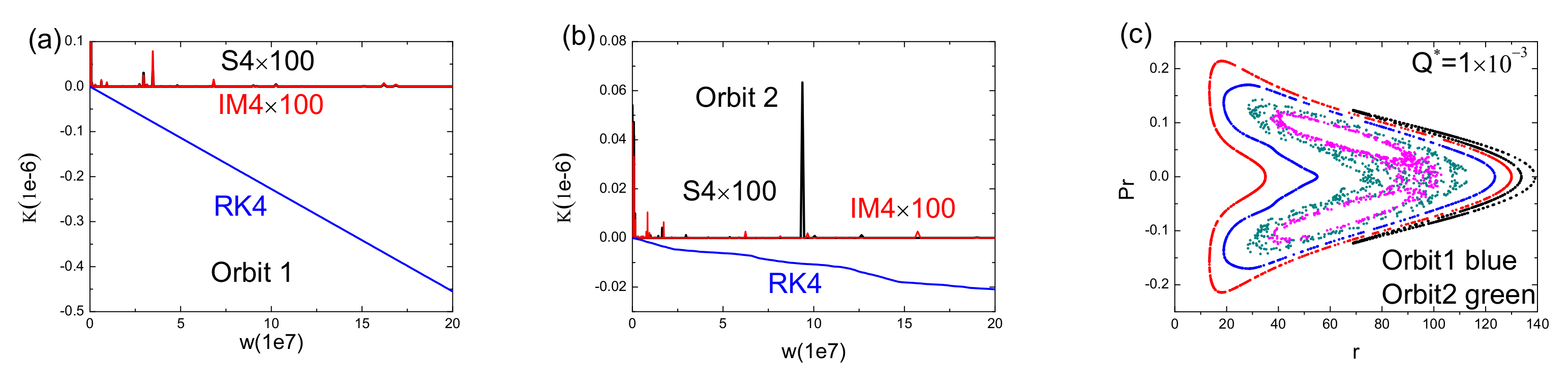
The detection of the chaotic behavior requires the adopted computational scheme with reliable results. Without a doubt, higher-order numerical integrators such as an eighth- and ninth-order Runge–Kutta–Fehlberg integrator with adaptive step sizes can yield high-precision numerical solutions. However, they are more computationally demanding than lower-order solvers. For Hamiltonian systems, the most appropriate solvers are symplectic integrators, which respect the symplectic nature of Hamiltonian dynamics and show no secular drift in energy errors [47,48,49,50,51,52,53]. A symplectic integrator method for numerical calculation of charged particle trajectory is well known due to its small error in energy even for long integration times, which make it perfectly suited for the description of regular and chaotic dynamics through Poincaré sections calculations [54]. Because the variables are inseparable in Hamiltonian systems associated with curved spacetimes, the standard explicit symplectic integrators do not work when these Hamiltonian systems are separated into two parts. In this case, completely implicit symplectic methods including the implicit midpoint method [55,56] and Gauss–Runge–Kutta methods [41,54,57,58] are often considered. Explicit and implicit combined symplectic methods [59,60,61,62,63] take less cost than these completely implicit methods and then are also used. Recently, explicit symplectic integrators were proposed for nonrotating black holes when the Hamiltonians of these black holes have several splitting parts with analytical solutions as explicit functions of proper time [64,65,66]. With the aid of time transformations, explicit symplectic integrators are easily available for the Kerr-type spacetimes [67].

The authors of [54] employed the Gauss–Legendre symplectic solver (i.e., s-stage implicit symplectic Runge–Kutta method) to study the regular and chaotic dynamics of charged particles around the Kerr background endowed with an axisymmetric electromagnetic test field with the aid of Poincaré sections. The authors of [68] applied the time-transformed explicit symplectic integrators introduced in [67] to mainly explore the effect of the black hole spin on the chaotic motion of a charged particle around the Kerr black hole immersed in an external electromagnetic field. Unlike Reference [68], the present work particularly focuses on how a small change in the black hole’s snductive charge [6] exerts influences on the effective potential, stable circular orbits and ISCOs on the equatorial plane, and a transition from order to chaos of orbits on the non-equatorial plane. The effects of other dynamical parameters such as the magnetic field parameter are also considered. For this purpose, we introduce a dynamical model for the description of charged particles moving around the Kerr black hole immersed in an external magnetic field in Section 2. The effective potential, stable circular orbits, and ISCOs on the equatorial plane are discussed in Section 3. The explicit symplectic integrators are designed for this problem, and the dependence of the orbital dynamical behavior on the parameters is shown in Section 4. Finally, the main results are summarized in Section 5.

2. Kerr Black Hole Immersed in External Magnetic Field

The Kerr black hole is the description of a rotating black hole with mass M and angular momentum a. In the standard Boyer–Lindquist coordinates $(t,r,\theta ,\varphi )$, its time-like metric is written as $d{s}^2=-c^{2}d{\tau }^2$, that is,

$$\begin{array}{ccc}\hfill d{s}^2& =& g_{\alpha \beta }d{x}^{\alpha }d{x}^{\beta }=g_{tt}{c}^{2}d{t}^2+2g_{t\varphi }cdtd\varphi \hfill \\ & & +g_{rr}d{r}^2+g_{\theta \theta }d{\theta }^2+g_{\varphi \varphi }d{\varphi }^2.\hfill \end{array}$$

(1)

These nonzero components in this metric are found in the paper of [69] as follows:

$$\begin{array}{ccc}\hfill g_{tt}& =& -(1-\frac{2GMr/c^2}{\mathrm{\Sigma }}),\hfill \\ \hfill g_{t\varphi }& =& -\frac{(2GMr/c^2)a{sin}^2\theta }{\mathrm{\Sigma }},\hfill \\ \hfill g_{rr}& =& \frac{\mathrm{\Sigma }}{\mathrm{\Delta }},g_{\theta \theta }=\mathrm{\Sigma },\hfill \\ \hfill g_{\varphi \varphi }& =& ({\rho }^2+\frac{2GMr}{\mathrm{\Sigma }}{a}^2{sin}^2\theta ){sin}^2\theta ,\hfill \end{array}$$

where $\mathrm{\Sigma }=r^2+a^2{cos}^2\theta$, $\mathrm{\Delta }={\rho }^2-2GMr/c^2$ and ${\rho }^2=r^2+a^2$. $\tau$ and t are proper and coordinate times, respectively. c is the speed of light, and G denotes the gravitational constant.

Suppose the Kerr black hole is immersed in an external asymptotically uniform magnetic field, which has strength B and yields an induced charge Q. Set ${\xi }_{\left(t\right)}^{\alpha }$ and ${\xi }_{\left(\varphi \right)}^{\alpha }$ as time-like and space-like axial Killing vectors. An electromagnetic four-vector potential can be found in References [6,70] and is written as

$$A^{\alpha }=aB{\xi }_{\left(t\right)}^{\alpha }+\frac{B}{2}{\xi }_{\left(\varphi \right)}^{\alpha }-\frac{Q}{2}{\xi }_{\left(t\right)}^{\alpha }.$$

(2)

This potential has two nonzero covariant components

$$\begin{array}{ccc}\hfill A_t& =& g_{t\alpha }{A}^{\alpha }=(aB-\frac{Q}{2})g_{tt}+\frac{B}{2}{g}_{t\varphi },\hfill \end{array}$$

(3)

$$\begin{array}{ccc}\hfill A_{\varphi }& =& g_{\varphi \alpha }{A}^{\alpha }=(aB-\frac{Q}{2})g_{t\varphi }+\frac{B}{2}{g}_{\varphi \varphi }.\hfill \end{array}$$

(4)

When $Q=2a{B}_w$, the inductive charge is the Wald charge $Q_W$, and $B_w$ is a magnetic field corresponding to the Wald charge [4]. The induced charge like the Wald charge $Q_W$ is so small that it has no contribution to the background geometry of the black hole [71]. However, the induced charge can exert an important influence on the motion of a charged particle under some circumstances, as will be shown in later discussions.

The motion of the particles around the rotating black hole embedded in the external magnetic field is described by the Hamiltonian

$$\begin{array}{ccc}\hfill H& =& \frac{1}{2m}{g}^{\mu \nu }(p_{\mu }-q{A}_{\mu })(p_{\nu }-q{A}_{\nu })\hfill \\ & =& \frac{H_1}{m}+\frac{1}{2m}\frac{\mathrm{\Delta }}{\mathrm{\Sigma }}{p}_r^2+\frac{1}{2m}\frac{p_{\theta }^2}{\mathrm{\Sigma }},\hfill \end{array}$$

(5)

where $p_r$ and $p_{\theta }$ are generalized momenta, and $H_1$ is a function of r and $\theta$ [68]:

$$\begin{array}{ccc}\hfill H_1& =& \frac{1}{2}{g}_{tt}{[f_1(E+q{A}_t)+f_2(L-q{A}_{\varphi })]}^2\hfill \\ & & +\frac{1}{2}{g}_{\varphi \varphi }{[f_2(E+q{A}_t)+f_3(L-q{A}_{\varphi })]}^2\hfill \\ & & -g_{t\varphi }[f_1(E+q{A}_t)+f_2(L-q{A}_{\varphi })]\hfill \\ & & ·[f_2(E+q{A}_t)+f_3(L-q{A}_{\varphi })].\hfill \end{array}$$

(6)

Here, $f_1$, $f_2$, and $f_3$ are functions of r and $\theta$ as follows:

$$\begin{array}{ccc}\hfill f_1& =& \frac{g_{\varphi \varphi }}{c^2(g_{tt}{g}_{\varphi \varphi }-g_{t\varphi }^2)},\hfill \end{array}$$

(7)

$$\begin{array}{ccc}\hfill f_2& =& \frac{g_{t\varphi }}{c(g_{tt}{g}_{\varphi \varphi }-g_{t\varphi }^2)},\hfill \end{array}$$

(8)

$$\begin{array}{ccc}\hfill f_3& =& \frac{g_{tt}}{g_{tt}{g}_{\varphi \varphi }-g_{t\varphi }^2}.\hfill \end{array}$$

(9)

$E=-p_t$ is a constant energy of the particle, and $L=p_{\varphi }$ is a constant angular momentum of the particle. $p_t$ and $p_{\varphi }$ are generalized momenta, which satisfy the relations

$$\begin{array}{ccc}& & \dot{t}=\frac{\partial H}{\partial p_t}=-f_1(E+q{A}_t)-f_2(L-q{A}_{\varphi }),\hfill \end{array}$$

(10)

$$\begin{array}{ccc}& & \dot{\varphi }=\frac{\partial H}{\partial p_{\varphi }}=f_2(E+q{A}_t)+f_3(L-q{A}_{\varphi }).\hfill \end{array}$$

(11)

Because the 4-velocity $U^{\alpha }=(c\dot{t},\dot{r},\dot{\theta },\dot{\varphi })$ is always identical to the constant $U^{\alpha }{U}_{\alpha }=-c^2$, the Hamiltonian (5) remains invariant and obeys the constraint

$$H=-\frac{1}{2}m{c}^2.$$

(12)

In fact, this third invariable quantity corresponds to the rest mass of the particle.

For simplicity, c and G take geometrized units: $c=G=1$. Dimensionless operations to the Hamiltonian (5) are carried out thorough a series of scale transformations: $r\to rM$, $t\to tM$, $\tau \to \tau M$, $a\to aM$, $E\to Em$, $p_r\to m{p}_r$, $L\to mML$, $p_{\theta }\to mM{p}_{\theta }$, $q\to mq$, $B\to B/M$ and $H\to mH$. Note that no scale transformation is given to the inductive charge Q. When these treatments are employed, M and m in all the above-mentioned expressions are eliminated or taken as geometrized units: $M=m=1$. The horizon event of the black hole exists for $\left|a\right|\le 1$. For convenience, we take $Q^{*}=qQ$ and $B^{*}=qB$.

3. Effective Potential and Stable Circular Orbits

Apart from the three integrals (10)–(12) in the dimensionless Hamiltonian (5), the fourth constant related to the particles’ azimuthal motion is absent in general when the external magnetic field forces are included. The absence of the fourth constant is mainly caused by the $g_{\varphi \varphi }$ term in Equation (4) rather than the $g_{tt}$ term in Equation (3). Because $g_{tt}$ is only a function of r, it does not destroy the presence of the fourth constant. However, $g_{\varphi \varphi }$ is a function of r and $\theta$, and therefore the Hamilton–Jacobi equation of Equation (5) has no separable form of variables r and $\theta$. This leads to the absence of the fourth constant. Of course, the $g_{t\varphi }$ terms, being functions of r and $\theta$ in Equations (3) and (4), also have some contributions to the absence of the fourth constant. In other words, the main contribution to the absence of the fourth constant in the (5) comes from the external magnetic fields associated with $B^{*}$. The inductive charges associated with $Q^{*}$ also exert some influences on the absence of the fourth constant. Thus, the dimensionless Hamiltonian (5) is non-integrable. However, it can be integrable for some particular cases. For instance, radial motions of charged particles on the equatorial plane $\theta =\pi /2$ are integrable. The radial motions are described in terms of effective potential V, i.e., the expression of E obtained from Equations (5) and (12) with $p_r=p_{\theta }=0$:

$$V=E=\frac{B}{2A}+\sqrt{\frac{B^2+4AC+2A}{4A^2}},$$

(13)

where A, B and C are expressed as

$$\begin{array}{ccc}\hfill A& =& -\frac{1}{2}(f_1^2{g}_{tt}+f_2^2{g}_{\varphi \varphi }-2f_1{f}_2{g}_{t\varphi }),\hfill \\ \hfill B& =& {\mathrm{B}}_1+{\mathrm{B}}_2+B_3,\hfill \\ \hfill C& =& \frac{1}{2}{g}_{tt}{C}_1+\frac{1}{2}{g}_{\varphi \varphi }{C}_2-g_{t\varphi }{C}_3,\hfill \\ \hfill B_1& =& g_{tt}q{A}_t{f}_1^2+g_{tt}{f}_1{f}_{2}L-g_{tt}{f}_1{f}_{2}q{A}_{\varphi },\hfill \\ \hfill B_2& =& g_{\varphi \varphi }q{A}_t{f}_2^2+g_{\varphi \varphi }{f}_2{f}_{3}L-g_{\varphi \varphi }{f}_2{f}_{3}q{A}_{\varphi },\hfill \\ \hfill B_3& =& -2g_{t\varphi }q{A}_t{f}_1{f}_2-g_{t\varphi }{f}_1{f}_{3}L+g_{t\varphi }q{A}_{\varphi }{f}_1{f}_3\hfill \\ & & -g_{t\varphi }{f}_2^{2}L+g_{t\varphi }q{A}_{\varphi }{f}_2^2,\hfill \\ \hfill C_1& =& f_1^2{q}^2{A}_t^2+2f_1{f}_{2}qL{A}_t-2f_1{f}_2{q}^2{A}_t{A}_{\phi }\hfill \\ & & +f_2^2\left(A_{\varphi }^2{q}^2-2A_{\varphi }Lq+L^2\right),\hfill \\ \hfill C_2& =& f_2^2{q}^2{A}_t^2+2f_2{f}_{3}qL{A}_t-2f_2{f}_3{q}^2{A}_t{A}_{\varphi }\hfill \\ & & +f_3^2\left(A_{\varphi }^2{q}^2-2A_{\varphi }Lq+L^2\right),\hfill \\ \hfill C_3& =& A_{\varphi }^2{f}_2{f}_3{q}^2-A_{\varphi }{A}_t{f}_1{f}_3{q}^2-A_{\varphi }{A}_t{f}_2^2{q}^2\hfill \\ & & +A_t^2{f}_1{f}_2{q}^2-2A_{\varphi }{f}_2{f}_{3}Lq+A_t{f}_1{f}_{3}Lq\hfill \\ & & +A_t{f}_2^{2}Lq+f_2{f}_3{L}^2.\hfill \end{array}$$

The local minimal values of the effective potential correspond to stable circular orbits, which satisfy the relation $dr/d\tau =0$ and the following conditions

$$\frac{dV}{dr}=0,$$

(14)

$$\frac{d^{2}V}{d{r}^2}\ge 0.$$

(15)

When the equality sign (=) is taken in Equation (15), the innermost stable circular orbit (ISCO) is present.

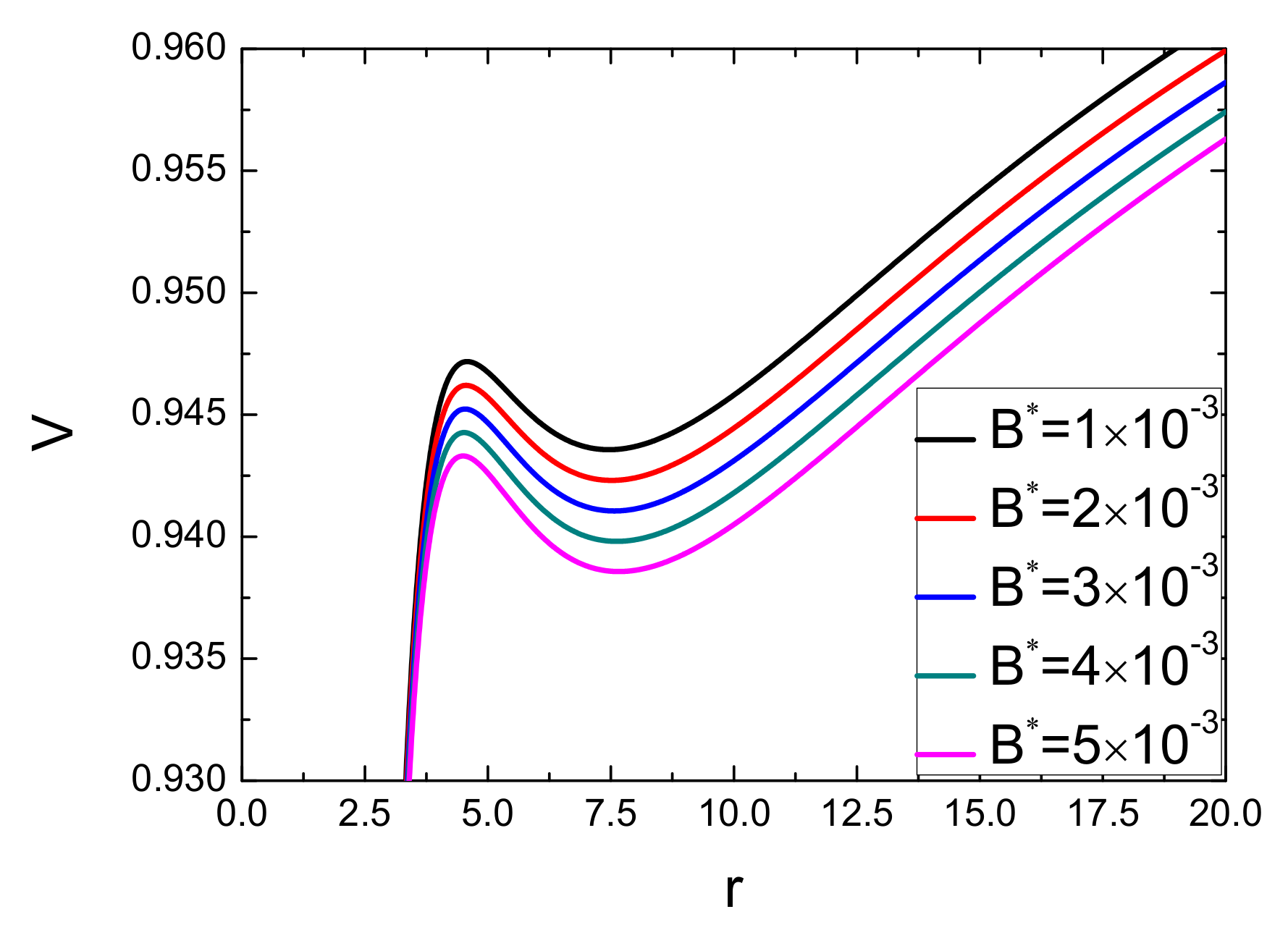
Taking parameters $L=2\sqrt{3}$, $a=0.1$, and $Q^{*}=2\times {10}^{-4}$ (if $q=0.1$ and $B_W=0.01$, then $Q=0.002$ is the Wald charge), we plot the effective potentials for several different magnetic parameters $B^{*}$ in Figure 1. When the magnetic parameter $B^{*}$ increases, the left shape of the effective potential goes away from the black hole, and the shape of the effective potential is not altered. The energies of the unstable or stable circular orbits become smaller. That is to say, the effective potential for a larger value of $B^{*}$ is below that for a smaller value of $B^{*}$. However, the radii of the stable circular orbits in

Table 1. Radii R of stable circular orbits in Figure 1.

Parameter	$B^{*}=0.001$	$B^{*}=0.002$	$B^{*}=0.003$	$B^{*}=0.004$
R	7.4595	7.5165	7.5693	7.6177
Parameter	$B^{*}=0.005$	$B^{*}=0.006$	$B^{*}=0.007$	$B^{*}=0.008$
R	7.6618	7.7013	7.7365	7.7673

get larger as $B^{*}$ increases.

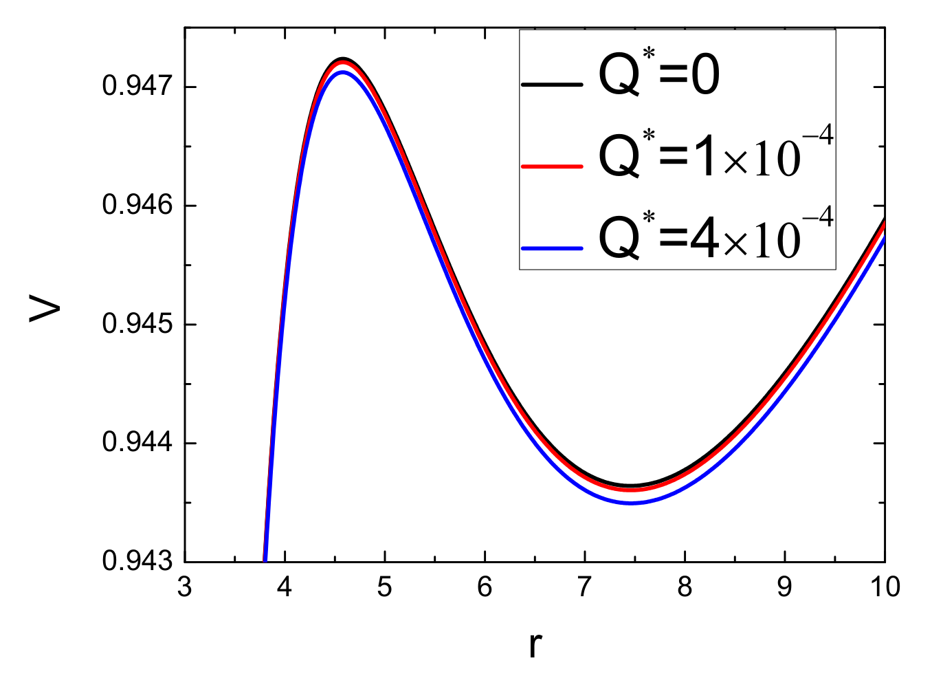
An increase in the inductive charge parameter $Q^{*}$ does not alter the shape of the effective potential but makes the left shape of the effective potential go away from the black hole in Figure 2. Meanwhile, the energies of the unstable or stable circular orbits decrease, but the radii of the stable circular orbits increase in

Table 2. Radii R of stable circular orbits. The related parameters are the same as those in Figure 2.

$\mathit{a}=0.1$	${\mathit{B}}^{*}=0.001$	${\mathit{B}}^{*}=0.002$
$Q^{*}=0$	7.4559	7.5129
$Q^{*}=0.0001$	7.4577	7.5147
$Q^{*}=0.0004$	7.4631	7.5201

.

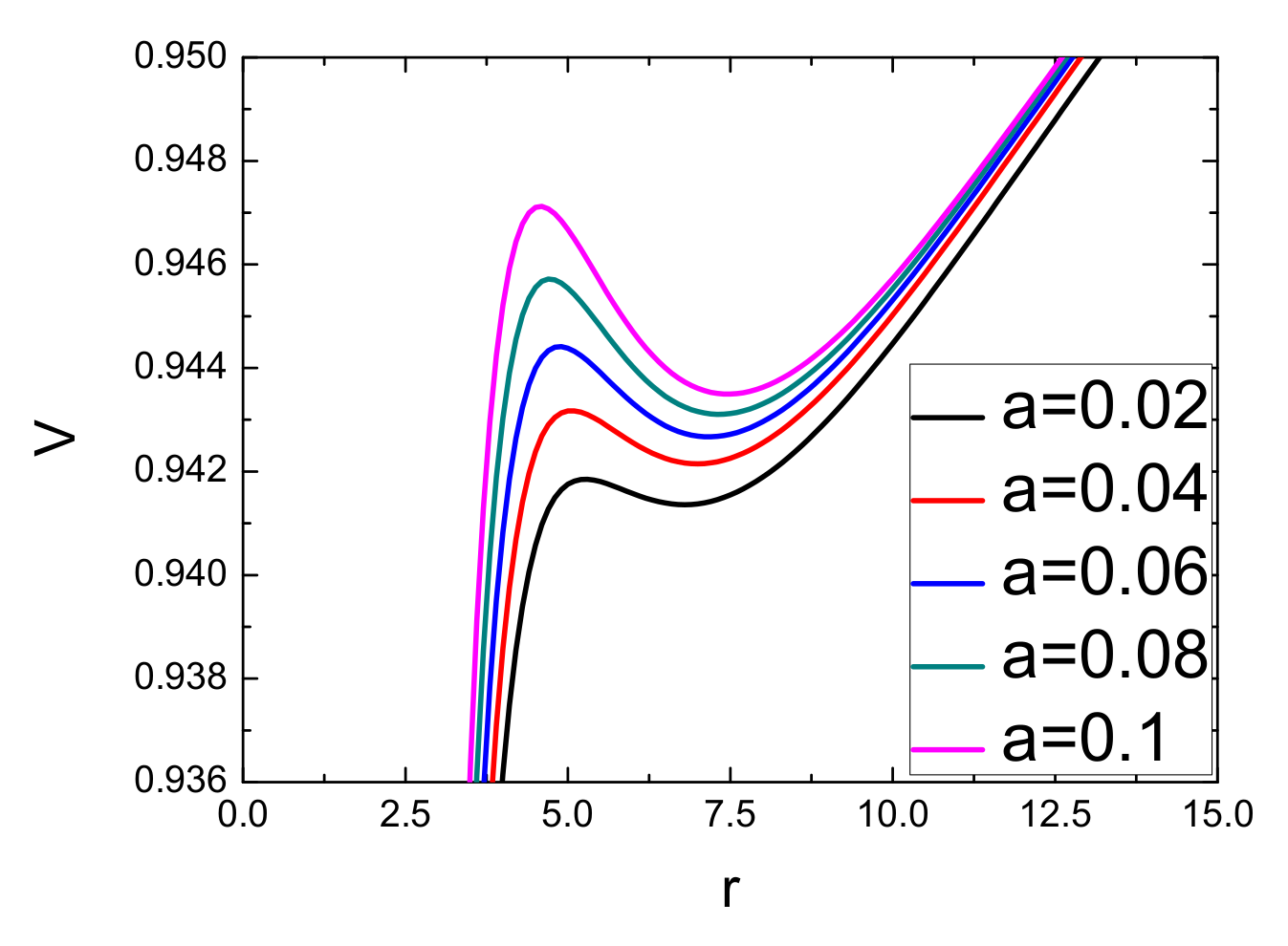
Figure 3 clearly describes the dependence of the effective potential on the black hole’s spin a. The energies of the stable circular orbits increase when a gets larger. The radii of the stable circular orbits always increase (see also

Table 3. Radii R of stable circular orbits in the Kerr spacetime of Figure 4. The radii R colored red are those of the innermost stable circular orbits (ISCOs).

a	L	R
	3.4641	6
0	4.0	12
	4.5	16.5876
	3.2640	5.3294
0.2	4.0	12.5329
	4.5	16.9761
	3.0340	4.6143
0.4	4.0	12.9954
	4.5	17.3336
	2.7559	3.8290
0.6	2.8	4.5721
	2.9	5.4096

).

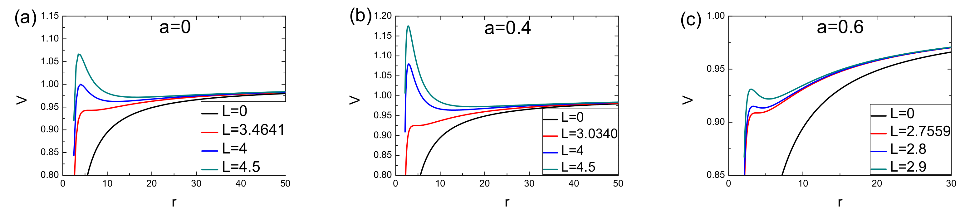
How does the effective potential vary as the particle’s angular momentum L increases? The effective potential for a larger value of L is always over that for a smaller value of L, as shown in the Kerr spacetime of Figure 4b,c. Note that there are critical values of L corresponding to the ISCOs colored red in Table 3, such as $L=3.4641$ for the Schwarzschild spacetime with $a=0$. When the angular momenta L are larger than the critical values, the stable circular orbits are present in Table 3. However, no stable circular orbits exist for L less than the critical values. As a or L increases, the radii of the stable circular orbits also increase.

Although the radii of the stable circular orbits increase with an increase in a, the radii of the ISCOs become smaller, as shown in Table 3. In addition, the radii of the ISCOs depend on the sign of the particle’s angular momentum as well as the magnitude of the particle’s angular momentum. When $L>0$ (for this case, the spin direction of the black hole is consistent with the particle’s angular momentum), the considered orbits are called direct orbits. When $L<0$ (for this case, the spin direction of the black hole is opposite to the particle’s angular momentum), the considered orbits are called retrograde orbits [38]. Given parameters a, $Q^{*}$ and $B^{*}$, the radii of the ISCOs for the retrograde orbits are larger than those for the direct orbits. If any one of the parameters a, $Q^{*}$, and $B^{*}$ increases, the radii of the ISCOs for the retrograde orbits or the direct orbits decrease. More details on the ISCOs are listed in

Table 4. Radii R of the ISCOs. The parameters are $a=0.2$, $Q^{*}=0.008$. DO represents a direct orbit, and RO denotes a retrograde orbit. Note that L with E is not arbitrarily given for the case of ISCOs, but it is for the case of stable circular orbits. R, E, and L are determined together in terms of the conditions of ISCOs.

	${\mathit{B}}^{*}=0.02$	${\mathit{B}}^{*}=0.02$	${\mathit{B}}^{*}=0.04$	${\mathit{B}}^{*}=0.04$	${\mathit{B}}^{*}=0.06$	${\mathit{B}}^{*}=0.06$
	DO	RO	DO	RO	DO	RO
R	5.2406	6.4737	5.0411	6.1176	4.7844	5.8262
L	3.1794	−3.8201	3.1433	−4.0808	3.1311	−4.3879
E	0.9078	0.9879	0.8885	1.0406	0.8726	1.10173

,

Table 5. Similar to Table 4, but the parameters are $a=0.2$ and $B^{*}=0.01$.

	${\mathit{Q}}^{*}=0$	${\mathit{Q}}^{*}=0$	${\mathit{Q}}^{*}=0.001$	${\mathit{Q}}^{*}=0.001$	${\mathit{Q}}^{*}=0.002$	${\mathit{Q}}^{*}=0.002$
	DO	RO	DO	RO	DO	RO
R	5.3276	6.599	5.3275	6.6193	5.3274	6.6043
L	3.2224	−3.7282	3.2209	−3.7265	3.2194	−3.7247
E	0.9226	0.9688	0.9222	0.9683	0.9217	0.9679

and

Table 6. Similar to Table 4, but the parameters are $a=0.2$ and $Q^{*}=0$.

	${\mathit{B}}^{*}=0$	${\mathit{B}}^{*}=0$	${\mathit{B}}^{*}=0.02$	${\mathit{B}}^{*}=0.02$	${\mathit{B}}^{*}=0.04$	${\mathit{B}}^{*}=0.04$
	DO	RO	DO	RO	DO	RO
R	5.3641	6.6713	5.2534	6.4653	5.0411	6.1218
L	3.2641	−3.6434	3.1912	−3.8343	3.1546	−4.0954
E	0.9354	0.9485	0.9112	0.9917	0.8918	1.0445

.

4. Numerical Investigations

Without loss of generality, the Hamiltonian system (5) for the description of the motion of charged particles at the non-equatorial plane is nonintegrable and has no analytical solutions. Numerical integration schemes are convenient to solve this system. Particularly for obtaining the numerical solutions of the Hamiltonian problem, symplectic integrators are naturally a prior choice. Because explicit symplectic integrators are generally superior to implicit ones at the same order in computational efficiency, their applications also remain a high priority. Owing to the difficulty in the separation of variables or the separation of two integrable parts in curved spacetimes, the implicit symplectic integrators rather than the explicit ones are suitably applicable to the curved spacetimes in general [41,54,55,56,57,58]. Recently, Wang et al. [64,65,66] split the Hamiltonians of non-rotating black holes surrounded by external magnetic fields into several parts with analytical solutions as explicit functions of proper time $\tau$, and successfully constructed the explicit symplectic integrators for these non-rotating black holes. More recently, the authors of [67] gave a time transformation to the Kerr geometry and designed the explicit symplectic integrators for the time-transformed Hamiltonian with a desired splitting form. The time-transformed explicit symplectic integrators were applied to study the dynamics of charged particles moving around the Kerr black hole surrounded by external magnetic fields without the inductive charge Q [68]. Following the two works [67,68], we use the explicit symplectic integrators to the Hamiltonian problem (5).

4.1. Explicit Symplectic Integrators

The authors of [67] introduced a time transformation function

$$d\tau =g(r,\theta )dw,g(r,\theta )=\frac{\mathrm{\Sigma }}{r^2},$$

(16)

where w is a new coordinate time unlike the original coordinate time t. The Hamiltonian (15) becomes

$$K=g(H+p_0)=\frac{\mathrm{\Sigma }}{r^2}(H_1+p_0)+\frac{\mathrm{\Delta }}{2r^2}{p}_r^2+\frac{1}{2r^2}{p}_{\theta }^2.$$

(17)

The new Hamiltonian K is a time-transformed Hamiltonian, where the proper time $\tau$ is viewed as a coordinate $q_0=\tau$ and its corresponding momentum is $p_0=-H=1/2\ne p_t$. In this case, K is always identical to zero for any coordinate time w, i.e.,

$$K\equiv 0.$$

(18)

Now, the time-transformed Hamiltonian K in Equation (17) is split into five parts

$$K=K_1+K_2+K_3+K_4+K_5,$$

(19)

where all sub-Hamiltonians are expressed as

$$\begin{array}{ccc}\hfill K_1& =& \frac{\mathrm{\Sigma }}{r^2}(H_1+p_0),\hfill \end{array}$$

(20)

$$\begin{array}{ccc}\hfill K_2& =& \frac{1}{2}{p}_r^2,\hfill \end{array}$$

(21)

$$\begin{array}{ccc}\hfill K_3& =& -\frac{1}{r}{p}_r^2,\hfill \end{array}$$

(22)

$$\begin{array}{ccc}\hfill K_4& =& \frac{a^2}{2r^2}{p}_r^2,\hfill \end{array}$$

(23)

$$\begin{array}{ccc}\hfill K_5& =& \frac{1}{2r^2}{p}_{\theta }^2.\hfill \end{array}$$

(24)

$K_2$, $K_3$, and $K_5$ are consistent with those of [67], but $K_1$ and $K_4$ are not.

Each of the five sub-Hamiltonians $K_1$, $K_2$, $K_3$, $K_4$, and $K_5$ is solved analytically, and its solutions are explicit functions of the new coordinate time w. Operators associated with the solutions of $K_1$, $K_2$, $K_3$, $K_4$, and $K_5$ are ${\widehat{K}}_1$, ${\widehat{K}}_2$, ${\widehat{K}}_3$, ${\widehat{K}}_4$, and ${\widehat{K}}_5$, respectively. The solutions of system (5) advancing a new coordinate time step $\mathrm{\Delta }w=h$ are given in terms of an explicit second-order symplectic integrator

$$\begin{array}{ccc}\hfill S_2^K\left(h\right)& =& {\widehat{K}}_5\left(\frac{h}{2}\right)\circ {\widehat{K}}_4\left(\frac{h}{2}\right)\circ {\widehat{K}}_3\left(\frac{h}{2}\right)\circ {\widehat{K}}_2\left(\frac{h}{2}\right)\circ {\widehat{K}}_1\left(h\right)\hfill \\ & & \circ {\widehat{K}}_2\left(\frac{h}{2}\right)\circ {\widehat{K}}_3\left(\frac{h}{2}\right)\circ {\widehat{K}}_4\left(\frac{h}{2}\right)\circ {\widehat{K}}_5\left(\frac{h}{2}\right),\hfill \end{array}$$

(25)

as was proposed in [67]. The second-order method easily yields a fourth-order symplectic integrator [72]

$$S_4^K\left(h\right)=S_2^K\left(\gamma h\right)\circ S_2^K\left(\delta h\right)\circ S_2^K\left(\gamma h\right),$$

(26)

where $\delta =1-2\gamma$ and $\gamma =1/(2-\sqrt[3]{2})$.

In fact, the explicit symplectic algorithms (25) and (26) are attributed to the development of the time-transformed symplectic method of [73] in the Kerr spacetime and its extension. The method of Mikkola [73] aims to exhibit good performance of symplectic integrators for close encounters of objects or high orbital eccentricities in the solar system. In the idea of Mikkola, these integrators use fixed time steps and remain symplectic for the new time but adaptive time steps for the original time. However, the time steps in the method of [67], including the present integrators (25) and (26), are approximately invariant for the proper time $\tau$ because $g\approx 1$ and $\mathrm{\Delta }\tau \approx g\mathrm{\Delta }w\approx \mathrm{\Delta }w=h$ for $r\gg 2$ in Equation (16). As the authors of [67] claimed, the time transformation mainly aims to eliminate the function $\mathrm{\Sigma }$ in the denominators of the terms $p_r$ and $p_{\theta }$ in the Hamiltonian H and to cause the time-transformed Hamiltonian K to have the desired separable form.

In comparison with S4, a fourth-order method implicit symplectic algorithm (IM4) consisting of three second-order implicit midpoint methods [56] is applied to the time-transformed Hamiltonian K. The conventional fourth-order Runge–Kutta explicit integration method (RK4) is also employed. Of course, IM4 and RK4 are suitable for the original Hamiltonian (5).

The new coordinate time step is given by $h=1$. The parameters are $E=0.9935$, $L=4.6$, $a=0.5$, $B^{*}=0.001$, and $Q^{*}=0.001$. The initial conditions are $\theta =\pi /2$ and $p_r=0$. If the initial separation r is given, then the initial value $p_{\theta }>0$ is obtained from Equation (12). We take $r=55$ for Orbit 1, and $r=75$ for Orbit 2. When the three algorithms S4, IM4, and RK4 independently integrate the two orbits in system (17), the evolutions of K in Equation (18) with integration time w are shown in Figure 5a,b. The explicit symplectic method S4 and the implicit symplectic algorithm IM4 do not show secular drifts in Hamiltonian errors, but RK4 does. In addition, S4 and IM4 are almost the same and have two orders of magnitude smaller errors than RK4. Accuracy of each algorithm for Orbit 2 in Figure 5b has an advantage over that for Orbit 1 in Figure 5a. Is this result because Orbit 2 is regular and Orbit 1 is chaotic? In fact, Orbit 1 is a regular Kolmogorov–Arnold–Moser (KAM) torus, but Orbit 2 exhibits the chaoticity, as described through Poincaré section at the plane $\theta =\pi /2$ with $p_{\theta }>0$ in Figure 5c. The result on the preference of accuracy of each algorithm for Orbit 2 over that for Orbit 1 is because Orbit 1 has a larger average period than Orbit 2. Although both orbits are not exactly periodic and Orbit 2 is chaotic, they have approximately average periods. Based on good computational efficiency, S4 is employed in the later studies.

4.2. Dynamics of Generic Orbits

Let us consider the effect of a small change in the inductive charge parameter $Q^{*}$ on the orbital dynamics. If $Q^{*}=0.001$ in Figure 5c gives place to $Q^{*}=0$, no chaos exists in Figure 6a. When $Q^{*}=0.0005$, all the orbits in Figure 6b are still regular. As the inductive charge parameter increases to $Q^{*}=0.0006$ in Figure 6c, the pink orbit with the initial separation $r=100$ is chaotic. For $Q^{*}=0.0008$ in Figure 6d, Orbit 2 and the pink orbit with the initial separation $r=100$ are chaotic. As the inductive charge parameter increases and takes the Wald charge $Q^{*}=2aBq=0.001$ in Figure 5c, chaos becomes stronger from the global phase-space structure. These facts show that a small increase in the inductive charge parameter $Q^{*}$ can easily induce chaos. An explanation of this result is given here. The inductive charges in the vicinity of the Wald charge are so small that they do not contribute to the spacetime curvature but can exert somewhat important influences on the motions of charged particles and even enhance the chaotic properties. The inductive charges have small contributions to the absence of the fourth constant, although the external magnetic fields provide the main contributions, as is claimed above. When $B^{*}$ is given an appropriate value and the ratio of the particle’s charge q to the particle’s mass m (i.e., $q/m$) is large enough, the inductive charges possibly contribute to the occurrence of chaos.

A minor change in the magnetic parameter $B^{*}$ has an important effect on the orbital dynamics. With $B^{*}$ increasing, the evolution of orbits transits from regular KAM tori for $B^{*}=0.0003$ in Figure 7a to chaos for $B^{*}=0.0008$ in Figure 7b and to stronger chaos for $B^{*}=0.0011$ in Figure 7c. An increase in $B^{*}$ means that of the Lorentz force and therefore enhances the strength of chaos.

The above demonstrations mainly consider how the two parameters $Q^{*}$ and $B^{*}$ exert influences on the orbital dynamical behavior. What about the effect of the black hole spin a on the orbital dynamics? Figure 8 gives an answer to this question. It is found that the chaotic properties are gradually weakened and ruled out as the dragging effects of the spacetime by the rotating black hole increase. This fact supports the result of [12]. It is shown again that an increase in the inductive charge parameter $Q^{*}$ helps to induce chaos for a given spin a. Similarly, an increase in the particle’s angular momentum L also results in weakening and suppressing the chaotic properties, as shown in Figure 9.

As is well known, chaos is stronger when the particle’s energy E is larger. This result is confirmed by fast Lyapunov indicators (FLIs) in Figure 10. Here, computations of the FLIs are based on the method of [74]. The FLI is the logarithm of the ratio of the separation between two nearby trajectories $d\left(\tau \right)$ at proper time $\tau$ to the starting separation $d\left(0\right)$:

$$FLI={log}_{10}\frac{d\left(\tau \right)}{d\left(0\right)}.$$

(27)

Different growths of separation $d\left(\tau \right)$ with proper time $\tau$ allow one to distinguish between ordered and chaotic orbits. A slowly polynomial or algebraical increase in the separation indicates the regularity of the considered bounded orbit for $E=0.9925$ in Figure 10. However, a rapidly exponential increase in the separation turns out to be the characteristic of chaoticness of the considered bounded orbit for $E=0.9935$. The FLI for $E=0.995$ is less than for $E=0.997$ after the integration time $w={10}^6$ or $\tau ={10}^6$; therefore, the former chaoticity is weaker than the latter one. That is, an increase of the energy E gives rise to enhancing strength of chaos.

We find that the FLIs are always smaller than 3.5 for the regular case but larger than this value for the chaotic case when the integration time reaches $w={10}^6$. Now, we employ the technique of FLIs to trace how a small variation in one parameter affects a dynamical transition from order to chaos. Only one of the parameters is given many different values, and the initial conditions (except $p_{\theta }$) and the other parameters are fixed. Each FLI is obtained after the integration time $w={10}^6$. The transition from order to chaos occurs when $Q^{*}\ge 0.00056$ (Figure 11a), $B^{*}\ge 0.000844$ (Figure 11b), or $E\ge 0.99379$ (Figure 11c). However, the transition from chaos to order occurs when $L\ge 5.84789$ (Figure 11d). That is, the strength of chaos is enhanced as one of the parameters $Q^{*}$, $B^{*}$, and E increases, but weakened as the parameter L increases. The effects of variations of these parameters on the orbital dynamics described by the technique of FLIs are consistent with those described by the technique of Poincaré sections.

The transition from order to chaos occurs when the black hole’s spin $a\ge 0.046$ in Figure 11e. That is, an increase in a leads to strong chaos. The result is consistent with that of [68], but unlike that of Figure 8, in which the dragging effects of the spacetime weaken the chaotic properties from the global phase-space structures. The different results between Figure 10 and Figure 11e are due to distinct choices of the initial conditions and other parameters. Perhaps, the dependence of the dynamical behavior on the spin may be different if the chosen initial conditions and other parameters are varied.

5. Conclusions

In this paper, we mainly focused on studying the dynamics of charged particles around the Kerr black hole immersed in an external electromagnetic field, which can be considered as a tidal environment.

First, we discussed the radial motions of charged particles on the equatorial plane through the effective potential. We traced how the dynamical parameters exert influences on the effective potential. It was found that the particle energies at the local maxima values of the effective potentials increase with an increase in the black hole spin and the particle angular momentum, whereas they decrease as one of the inductive charge parameter and magnetic field parameter increases. In addition, the radii of stable circular orbits on the equatorial plane always increase. However, the radii of ISCOs decrease as any one of the black hole spin $\left|a\right|$, inductive charge parameter $Q^{*}$, and uniform magnetic field parameter $B^{*}$ is increasing.

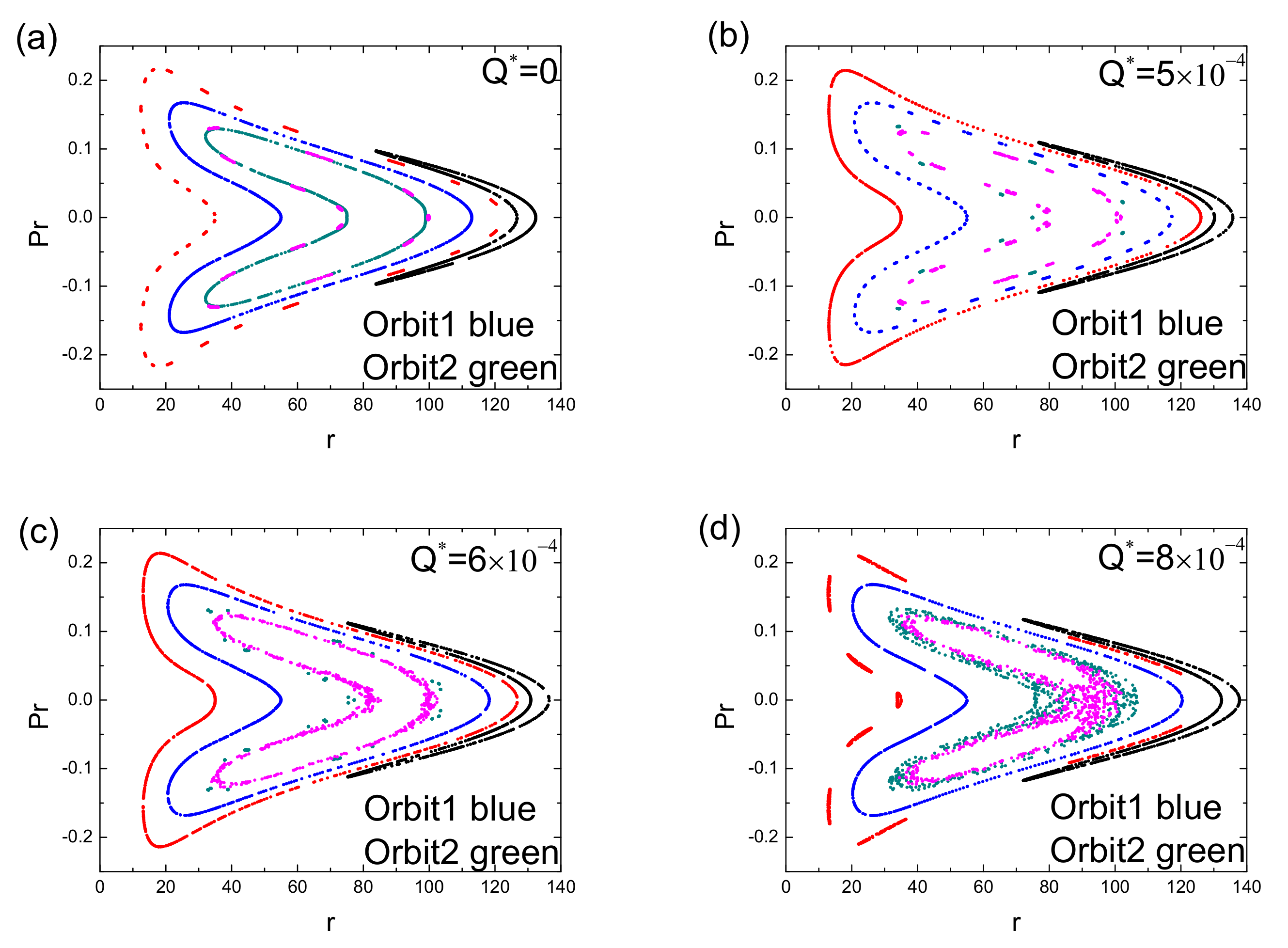
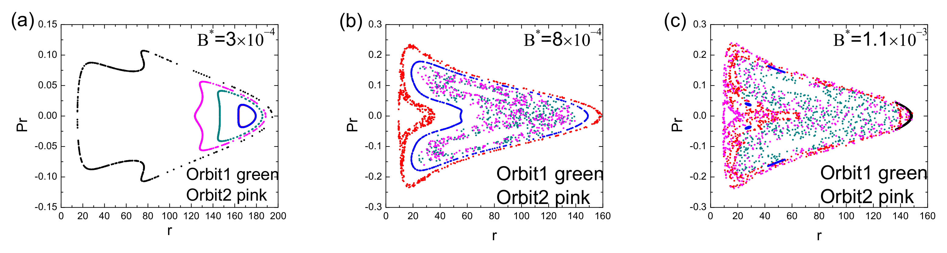
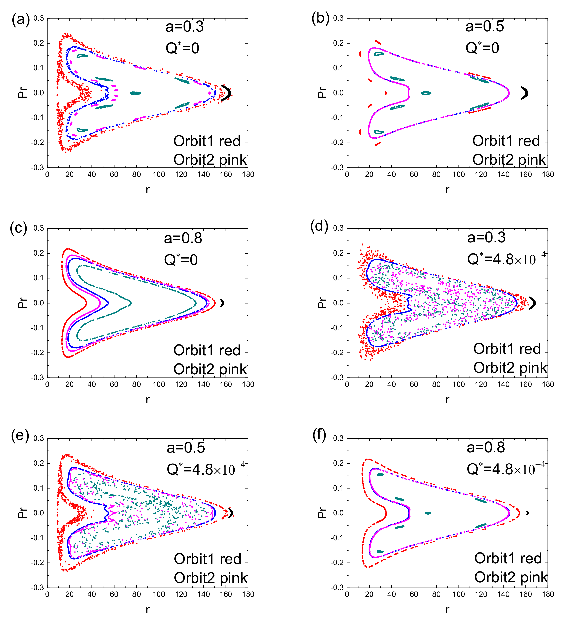
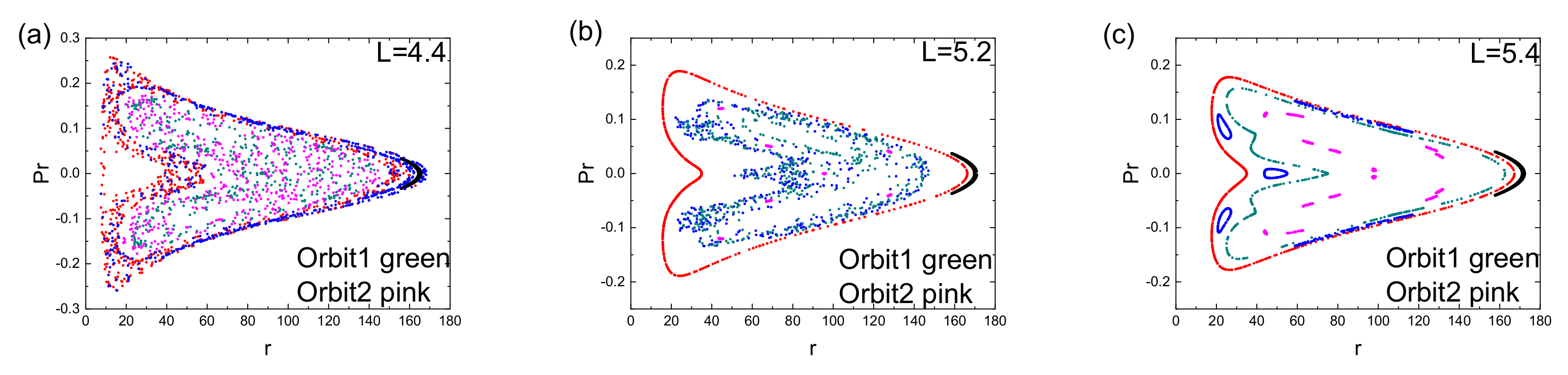
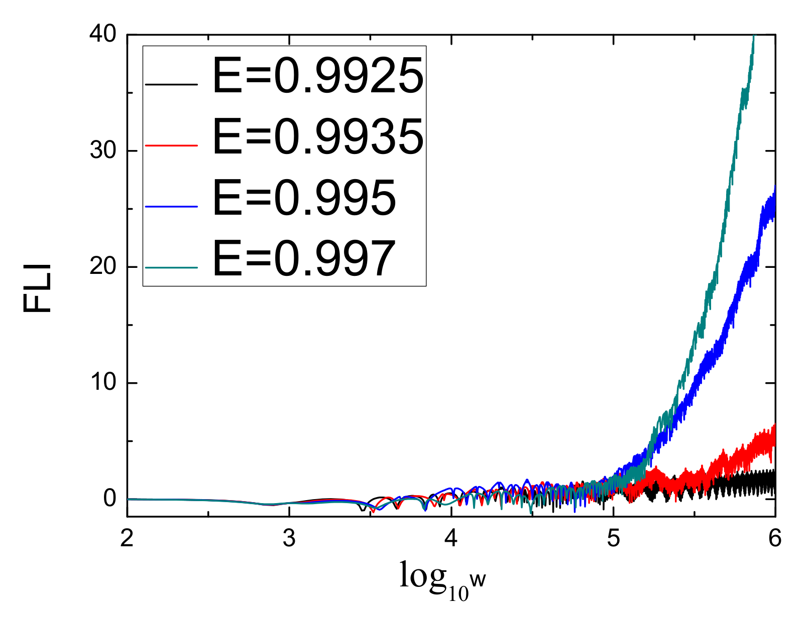
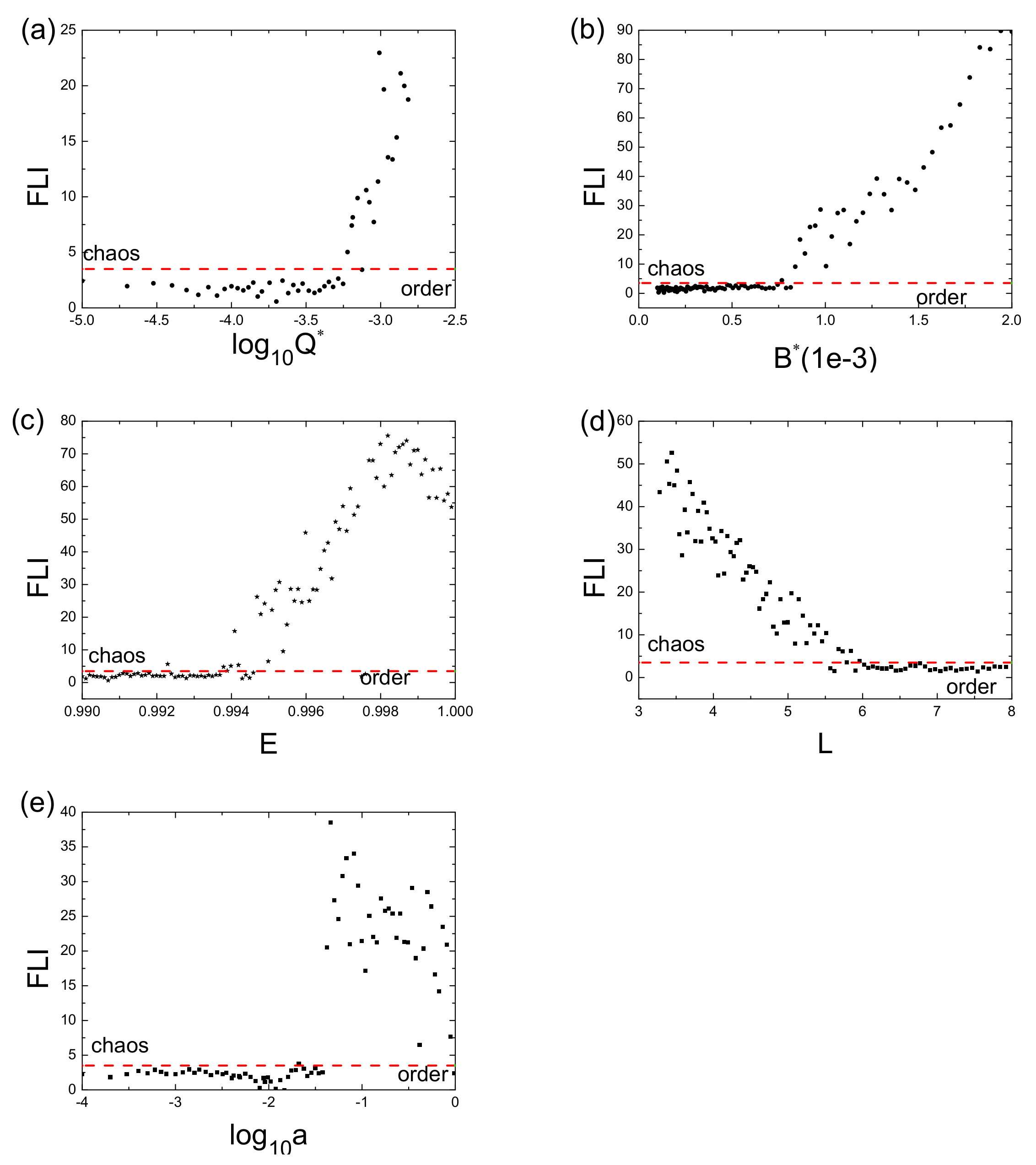
Then, we investigated the motions of charged particles on the non-equatorial plane using a time-transformed explicit symplectic integrator. The effects of small variations of the parameters on the orbital regular and chaotic dynamics are studied through the techniques of Poincaré sections and fast Lyapunov indicators. As a result, the dynamics have sensitive dependence on a small variation in any one of the inductive charge parameter, magnetic field parameter, energy, and angular momentum. Chaos is easily induced as the inductive charge parameter, magnetic field parameterm and energy increase but weakened as the angular momentum increases. When the dragging effects of the spacetime increase, the chaotic properties are not always enhanced or weakened under some circumstances.

The theoretical work may have potential astrophysical applications. The unstable or stable circular orbits and ISCOs would be helpful to study some accretion disks. The theory of chaotic scattering in the combined effective potential and the asymptotically uniform magnetic field would be applicable to explaining the mechanism hidden behind the charged particle ejection. The existence of the magnetic fields involving the induced electric field may be demonstrated through observational evidence.

References

1. Akiyama, K.; Alberdi, A.; Alef, W.; Asada, K.; Azulay, R.; Baczko, A.K.; Ball, D.; Baloković, M.; Barrett, J.; Bintley, D.; et al. First M87 Event Horizon Telescope Results. IV. Imaging the Central Supermassive Black Hole. Astrophys. J. 2019, 875, L4. [Google Scholar]
2. Carter, B. Global Structure of the Kerr Family of Gravitational Fields. Phys. Rev. 1968, 174, 1559. [Google Scholar] [CrossRef] [Green Version]
3. Eatough, R.P.; Falcke, H.; Karuppusamy, R.; Lee, K.J.; Champion, D.J.; Keane, E.F.; Desvignes, G.; Schnitzeler, D.H.F.M.; Spitler, L.G.; Kramer, M.; et al. A strong magnetic field around the supermassive black hole at the centre of the Galaxy. Nature 2013, 501, 391–394. [Google Scholar] [CrossRef] [PubMed] [Green Version]
4. Wald, R.M. Black hole in a uniform magnetic field. Phys. Rev. D 1974, 6, 1068. [Google Scholar] [CrossRef]
5. Stuchlík, Z.; Kološ, M. Acceleration of the charged particles due to chaotic scattering in the combined black hole gravitational field and asymptotically uniform magnetic field. Eur. Phys. J. C 2016, 76, 32. [Google Scholar] [CrossRef] [Green Version]
6. Tursunov, A.; Stuchlík, Z.; Kološ, M. Circular orbits and related quasiharmonic oscillatory motion of charged particles around weakly magnetized rotating black holes. Phys. Rev. D 2016, 93, 084012. [Google Scholar] [CrossRef] [Green Version]
7. Rayimbaev, J.R. Magnetized particle motion around non-Schwarzschild black hole immersed in an external uniform magnetic field. Astrophys. Space Sci. 2016, 361, 288. [Google Scholar] [CrossRef]
8. Bambi, C.; Barausse, E. Final stages of accretion onto non-Kerr compact objects. Phys. Rev. D 2011, 84, 084034. [Google Scholar] [CrossRef] [Green Version]
9. Chowdhury, A.N.; Patil, M.; Malafarina, D.; Joshi, P.S. Circular geodesics and accretion disks in the Janis-Newman-Winicour and gamma metric spacetimes. Phys. Rev. D 2012, 85, 104031. [Google Scholar] [CrossRef] [Green Version]
10. Liang, E.P.T. Equatorial circular orbits of some static gravitational fields with naked singularities. Phys. Rev. D 1974, 9, 3257. [Google Scholar] [CrossRef]
11. Aliev, A.; <i>o</i>¨zdemir, N. Motion of charged particles around a rotating black hole in a magnetic field. Mon. Not. R. Astron. Soc. 2002, 336, 241–248. [Google Scholar] [CrossRef] [Green Version]
12. Takahashi, M.; Koyama, H. Chaotic motion of charged particles in an electromagnetic field surrounding a rotating black hole. Astrophys. J. 2009, 693, 472. [Google Scholar] [CrossRef] [Green Version]
13. Pradhan, P.; Majumdar, P. Circular orbits in extremal Reissner-Nordstrom spacetime. Phys. Lett. A 2011, 375, 474–479. [Google Scholar] [CrossRef] [Green Version]
14. Gladush, V.D.; Galadgyi, M.V. Some peculiarities of motion of neutral and charged test particles in the field of a spherically symmetric charged object in general relativity. Gen. Relat. Gravit. 2011, 43, 1347–1363. [Google Scholar] [CrossRef] [Green Version]
15. Pugliese, D.; Quevedo, H.; Ruffini, R. Circular motion of neutral test particles in Reissner-Nordstrom spacetime. Phys. Rev. D 2011, 83, 024021. [Google Scholar] [CrossRef] [Green Version]
16. Pugliese, D.; Quevedo, H.; Ruffini, R. Equatorial circular motion in Kerr spacetime. Phys. Rev. D 2011, 84, 044030. [Google Scholar] [CrossRef] [Green Version]
17. Pugliese, D.; Quevedo, H.; Ruffini, R. Motion of charged test particles in Reissner-Nordstrom spacetime. Phys. Rev. D 2011, 83, 104052. [Google Scholar] [CrossRef] [Green Version]
18. Stuchl<i>i</i>´k, Z.; Kolo<i>s</i>˘, M. String loops in the field of braneworld spherically symmetric black holes and naked singularities. J. Cosmol. Astropart. Phys. 2012, 10, 8. [Google Scholar]
19. Patil, M.; Joshi, P.S. Acceleration of particles by Janis-Newman-Winicour singularities. Phys. Rev. D 2012, 85, 104014. [Google Scholar] [CrossRef] [Green Version]
20. Kopáček, O.; Karas, V. Inducing chaos by breaking axial symmetry in a black hole magnetosphere. Astrophys. J. 2014, 787, 117. [Google Scholar] [CrossRef] [Green Version]
21. Lim, Y.-K. Motion of charged particles around a magnetized/electrified black hole. Phys. Rev. D 2015, 91, 024048. [Google Scholar] [CrossRef] [Green Version]
22. Kolos, M.; Stuchlík, Z.; Tursunov, A. Quasi-harmonic oscillatory motion of charged particles around a Schwarzschild black hole immersed in a uniform magnetic field. Class. Quantum Gravity 2015, 32, 165009. [Google Scholar] [CrossRef] [Green Version]
23. Panis, R.; Kološ, M.; Stuchlík, Z. Determination of chaotic behaviour in time series generated by charged particle motion around magnetized Schwarzschild black holes. Eur. Phys. C 2019, 79, 479. [Google Scholar] [CrossRef] [Green Version]
24. Bokhari, A.H.; Rayimbaev, J.; Ahmedov, B. Test particles dynamics around deformed Reissner-Nordström black hole. Phys. Rev. D 2020, 102, 124078. [Google Scholar] [CrossRef]
25. Igata, T.; Ishihara, H.; Takamori, Y. Stable Bound Orbits of Massless Particles around a Black Ring. Phys. Rev. D 2013, 87, 104005. [Google Scholar] [CrossRef] [Green Version]
26. Igata, T. Stable bound orbits in six-dimensional Myers-Perry black holes. Phys. Rev. D 2015, 92, 024002. [Google Scholar] [CrossRef] [Green Version]
27. Rincón, Á.; Panotopoulos, G.; Lopes, I.; Cruz, N. ISCOs and OSCOs in the Presence of a Positive Cosmological Constant in Massive Gravity. Universe 2021, 7, 278. [Google Scholar] [CrossRef]
28. Schroven, K.; Grunau, S. The ISCO of charged particles in Reissner-Nordström, Kerr–Newman and Kerr-Sen spacetime. Phys. Rev. D 2021, 103, 024016. [Google Scholar] [CrossRef]
29. Koch, B.; Saueressig, F. Black holes within asymptotic safety. Int. J. Modern Phys. A 2014, 29, 1430011. [Google Scholar] [CrossRef] [Green Version]
30. Cristopher, G.; Benjamin, K. Improved Reissner-Nordström-(A)dS Black Hole in Asymptotic Safety. Int. J. Modern Phys. A 2016, 31, 1650141. [Google Scholar]
31. Koch, B.; Reyes, I.A.; Rincoén, Á. A scale dependent black hole in three-dimensional space-time. Class. Quantum Gravity 2016, 33, 225010. [Google Scholar] [CrossRef]
32. Brans, C.; Dicke, R.H. Mach’s Principle and a Relativistic Theory of Gravitation. Phys. Rev. 1961, 124, 925. [Google Scholar] [CrossRef]
33. Brans, C. Mach’s Principle and a Relativistic Theory of Gravitation. II. Phys. Rev. 1961, 125, 2194. [Google Scholar] [CrossRef]
34. Bonanno, A.; Reuter, M. Renormalization group improved black hole spacetimes. Phys. Rev. D 2000, 62, 043008. [Google Scholar] [CrossRef] [Green Version]
35. Rincó, Á.; Panotopoulos, G. Quasinormal modes of scale dependent black holes in (1+2)-dimensional Einstein-power-Maxwell theory. Phys. Rev. D 2018, 97, 024027. [Google Scholar] [CrossRef] [Green Version]
36. Hackmann, E.; Xu, H. Charged particle motion in Kerr–Newmann space-times. Phys. Rev. D 2013, 87, 124030. [Google Scholar] [CrossRef] [Green Version]
37. Esteban, E.P.; Ramos, E. Rotating black hole in an external electromagnetic field. Phys. Rev. D 1988, 38, 2963. [Google Scholar] [CrossRef]
38. Esteban, E.P.; Medina, I.R. Accretion onto black holes in external magnetic fields. Phys. Rev. D 1990, 42, 307. [Google Scholar] [CrossRef]
39. Karas, V.; Vokrouhlicky, D. Chaotic motion of test particles in the Ernst space-time. Gen. Relat. Gravit. 1992, 24, 729–743. [Google Scholar] [CrossRef]
40. Nakamura, Y.; Ishizuka, T. Motion of a Charged Particle Around a Black Hole Permeated by Magnetic Field and its Chaotic Characters. Astrophys. Space Sci. 1993, 210, 105–108. [Google Scholar] [CrossRef]
41. Kopáček, O.; Karas, V.; Kovář, J.; Stuchlík, Z. Transition from regular to chaotic circulation in magnetized coronae near compact objects. Astrophys. J. 2010, 722, 1240. [Google Scholar] [CrossRef]
42. Liu, L.; Wu, X.; Huang, G.Q.; Liu, F. Higher order explicit symmetric integrators for inseparable forms of coordinates and momenta. Mon. Not. R. Astron. Soc. 2016, 459, 1968–1976. [Google Scholar] [CrossRef] [Green Version]
43. Kopáček, O.; Karas, V. Near-horizon Structure of Escape Zones of Electrically Charged Particles around Weakly Magnetized Rotating Black Hole. Astrophys. J. 2018, 853, 53. [Google Scholar] [CrossRef] [Green Version]
44. Li, D.; Wu, X. Chaotic motion of neutral and charged particles in a magnetized Ernst-Schwarzschild spacetime. Eur. Phys. J. Plus. 2019, 134, 96. [Google Scholar] [CrossRef] [Green Version]
45. Stuchlí, Z.; Kološ, M.; Kovář, J.; Slaný, P.; Tursunov, A. Influence of Cosmic Repulsion and Magnetic Fields on Accretion Disks Rotating around Kerr Black Holes. Universe 2020, 6, 26. [Google Scholar] [CrossRef] [Green Version]
46. Yi, M.; Wu, X. Dynamics of charged particles around a magnetically deformed Schwarzschild black hole. Phys. Scr. 2020, 95, 085008. [Google Scholar] [CrossRef]
47. Swope, W.C.; Andersen, H.C.; Berens, P.H.; Wilson, K.R. A computer simulation method for the calculation of equilibrium constants for the formation of physical clusters of molecules: Application to small water clusters. J. Chem. Phys. 1982, 76, 637–649. [Google Scholar] [CrossRef]
48. Wisdom, J. The origin of the Kirkwood gaps-A mapping for asteroidal motion near the 3/1 commensurability. Astron. J. 1982, 87, 577–593. [Google Scholar] [CrossRef]
49. Ruth, R.D. A canonical integration technique. IEEE Trans. Nuclear Sci. 1983, 30, 2669–2671. [Google Scholar] [CrossRef]
50. Forest, E.; Ruth, R.D. Fourth-order symplectic integration. Phys. D 1990, 43, 105–117. [Google Scholar] [CrossRef] [Green Version]
51. Wisdom, J.; Holman, M. Symplectic maps for the n-body problem. Astron. J. 1991, 102, 1528–1538. [Google Scholar] [CrossRef]
52. Chambers, J.E.; Murison, M.A. Pseudo-High-Order Symplectic Integrators. Astron. J. 2000, 19, 425. [Google Scholar] [CrossRef] [Green Version]
53. Laskar, J.; Robutel, P. High order symplectic integrators for perturbed Hamiltonian systems. Celest. Mech. Dyn. Astronomy 2001, 80, 39L. [Google Scholar] [CrossRef]
54. Kopáček, O.; Karas, V.; Kovář, J.; Stuchlík, Z. Application of a symplectic integrator in a non-integrable relativistic system. arXiv 2016, arXiv:1601.01262. [Google Scholar]
55. Feng, K. Symplectic geometry and numerical methods in fluid dynamics. Lecture Notes Phys. 1986, 264, 1–7. [Google Scholar]
56. Brown, J.D. Midpoint rule as a variational-symplectic integrator: Hamiltonian systems. Phys. Rev. D 2006, 73, 024001. [Google Scholar] [CrossRef] [Green Version]
57. Seyrich, J.; Lukes-Gerakopoulos, G. Symmetric integrator for nonintegrable Hamiltonian relativistic systems. Phys. Rev. D 2012, 86, 124013. [Google Scholar] [CrossRef] [Green Version]
58. Seyrich, J. Gauss collocation methods for efficient structure preserving integration of post-Newtonian equations of motion. Phys. Rev. D 2013, 87, 084064. [Google Scholar] [CrossRef] [Green Version]
59. Preto, M.; Saha, P. On post-Newtonian orbits and the Galactic-center stars. Astrophys. J. 2009, 703, 1743. [Google Scholar] [CrossRef] [Green Version]
60. Lubich, C.; Walther, B.; Brügmann, B. Symplectic integration of post-Newtonian equations of motion with spin. Phys. Rev. D 2010, 81, 104025. [Google Scholar] [CrossRef] [Green Version]
61. Zhong, S.Y.; Wu, X.; Liu, S.Q.; Deng, X.F. Global symplectic structure-preserving integrators for spinning compact binaries. Phys. Rev. D 2010, 82, 124040. [Google Scholar] [CrossRef]
62. Mei, L.; Ju, M.; Wu, X.; Liu, S. Dynamics of spin effects of compact binaries. Mon. Not. R. Astron. Soc. 2013, 435, 2246–2255. [Google Scholar] [CrossRef] [Green Version]
63. Mei, L.; Wu, X.; Liu, F. On preference of Yoshida construction over Forest-Ruth fourth-order symplectic algorithm. Eur. Phys. J. C 2013, 73, 2413. [Google Scholar] [CrossRef]
64. Wang, Y.; Sun, W.; Liu, F.Y.; Wu, X. Construction of Explicit Symplectic Integrators in General Relativity. I. Schwarzschild Black Holes. Astrophys. J. 2021, 907, 66. [Google Scholar] [CrossRef]
65. Wang, Y.; Sun, W.; Liu, F.Y.; Wu, X. Construction of Explicit Symplectic Integrators in General Relativity. II. Reissner-Nordström Black Holes. Astrophys. J. 2021, 909, 22. [Google Scholar] [CrossRef]
66. Wang, Y.; Sun, W.; Liu, F.Y.; Wu, X. Construction of Explicit Symplectic Integrators in General Relativity. III. Reissner-Nordström-(anti)-de Sitter Black Holes. Astrophys. J. Suppl. Ser. 2021, 254, 8. [Google Scholar] [CrossRef]
67. Wu, X.; Wang, Y.; Sun, W.; Liu, F.Y. Construction of Explicit Symplectic Integrators in General Relativity. IV. Kerr Black Holes. Astrophys. J. 2021, 914, 63. [Google Scholar] [CrossRef]
68. Sun, W.; Wang, Y.; Liu, F.Y.; Wu, X. Applying explicit symplectic integrator to study chaos of charged particles around magnetized Kerr black hole. Eur. Phys. J. C 2021, 81, 785. [Google Scholar] [CrossRef]
69. Newman, E.T.; Couch, E.; Chinnapared, K.; Exton, A.; Prakash, A.; Torrence, R. Metric of a Rotating, Charged Mass. J. Math. Phys. 1965, 6, 918–919. [Google Scholar] [CrossRef]
70. Kovář, J.; Kopáček, O.; Karas, V.; Stuchlák, Z. Off-equatorial orbits in strong gravitational fields near compact objects—II: Halo motion around magnetic compact stars and magnetized black holes. Class. Quantum Gravity 2010, 27, 135006. [Google Scholar] [CrossRef]
71. Zajaček, M.; Tursunov, A.; Eckart, A.; Britzen, S.; Hackmann, E.; Karas, V.; Stuchlík, Z.; Czerny, B.J. Anton Zensus. Constraining the charge of the Galactic centre black hole. J. Phys. Conf. Ser. 2019, 1258, 012031. [Google Scholar] [CrossRef]
72. Yoshida, H. Construction of higher order symplectic integrators. Phys. Lett. A 1990, 150, 262–268. [Google Scholar] [CrossRef]
73. Mikkola, S. Practical symplectic methods with time transformation for the few-body problem. Celest. Mech. Dyn. Astronomy 1997, 67, 145–165. [Google Scholar] [CrossRef]
74. Wu, X.; Huang, T.Y.; Zhang, H. Lyapunov indices with two nearby trajectories in a curved spacetime. Phys. Rev. D 2006, 74, 083001. [Google Scholar] [CrossRef] [Green Version]
Figure 1. Effective potentials for different uniform magnetic field parameters B * . The other parameters are L = 2 3 , a = 0.1 , and Q * = 0.0002 .
Universe 07 00410 g001
Figure 2. Effective potentials for several inductive charge parameters Q * . The other parameters are B * = 0.001 , a = 0.1 and L = 2 3 .
Universe 07 00410 g002
Figure 3. Effective potentials for several black hole spins a. The other parameters are L = 2 3 , B * = 0.001 and Q * = 0.004 .
Universe 07 00410 g003
Figure 4. The black hole spins are (a) a = 0, (b) a = 0.4 and (c) a = 0.6. Effective potentials for different angular momenta L of test particles. The other parameters are Q * = 0 and B * = 0 .
Universe 07 00410 g004
Figure 5. (a,b): Accuracies of the time-transformed Hamiltonian K yielded by three methods S4, IM4, and RK4 acting on Orbit 1 and Orbit 2. The time-step is h = 1 . Orbits 1 and 2 have their initial separations r = 55 and r = 75 , respectively. The other initial conditions are θ = π / 2 , p r = 0 and p θ > 0 . The parameters are E = 0.9935 , L = 4.6 , B * = 0.001 , a = 0.5 , and Q * = 0.001 . Symbol “ × 100 ” means that the plotted errors are enlarged 100 time compared with the practical errors. (c) Poincaré sections at plane θ = π / 2 with p θ > 0 . The black orbit has its initial separation r = 25 , the red orbit has the initial separation r = 35 , and the pink orbit has the initial separation r = 100 . Orbit 1 is regular, whereas Orbit 2 and the pink orbit with the initial separation r = 100 are chaotic.
Universe 07 00410 g005
Figure 6. Same as Figure 5c but the inductive charge parameters Q * are different. There is no chaos in (a,b). Chaos occurs for the pink orbit with the initial separation r = 100 in (c). Orbit 2 and the pink orbit with the initial separation r = 100 are chaotic in (d).
Universe 07 00410 g006
Figure 7. Poincaré sections. The magnetic field parameters are (a) B* = 0.0003, (b) B* = 0.0008 and (c) B* = 0.0011. The parameters are E = 0.995 , L = 4.6 , a = 0.5 , and Q * = 0.0003 . Orbits 1 and 2 have their initial separations r = 75 and r = 100 , respectively. The initial separations are r = 15 for the black orbit, r = 35 for the red orbit, and r = 55 for the blue orbit.
Universe 07 00410 g007
Figure 8. Poincaré sections. The parameters are E = 0.995 , L = 4.6 , and B * = 0.0008 . Orbits 1 and 2 have their initial separations r = 35 and r = 145 , respectively. The initial separations are r = 15 for the black orbit, r = 55 for the blue orbit, and r = 75 for the green orbit. (ac) have the same spins a = 0 but different charge parameters Q*. (df) have the same spins a = 0.00048 but different charge parameters Q*.
Universe 07 00410 g008
Figure 9. Poincaré sections. The parameters are E = 0.995 , a = 0.1 , B * = 8 × 10 4 , and Q * = 1 × 10 5 . Orbits 1 and 2 have their initial separations r = 75 and r = 95 , respectively. The initial separations are r = 15 for the black orbit, r = 35 for the red orbit, and r = 55 for the blue orbit. The angular momenta in (ac) are different.
Universe 07 00410 g009
Figure 10. Fast Lyapunov indicators (FLIs). The parameters are L = 4.6 , a = 0.5 , B * = 0.001 , and Q * = 0.001 . The initial separation is r = 75 .
Universe 07 00410 g010
Figure 11. Dependence of FLIs on the parameters. Each of the FLIs is obtained after the integration time w = 10 6 . The parameters and initial separations are as follows. (a) E = 0.9935 , L = 4.6 , a = 0.5 , B * = 0.001 , and r = 100 . (b) E = 0.995 , L = 4.6 , a = 0.5 , Q * = 0.0001 , and r = 75 . (c) L = 4.6 , a = 0.5 , B * = 1 × 10 3 , Q * = 1.25 × 10 4 , and r = 75 . (d) E = 0.995 , a = 0.5 , B * = 1 × 10 3 , Q * = 1.25 × 10 4 , and r = 75 . (e) E = 0.995 , L = 4.6 , B * = 1 × 10 3 , Q * = 2 × 10 7 , and r = 75 .
Universe 07 00410 g011