
A Hybrid Bald Eagle Search Algorithm for Time Difference of Arrival Localization


1
Electrical Engineering College, Guizhou University, Guiyang 550025, China
2
Power China Guizhou Engineering Co., Ltd., Guiyang 550001, China
3
Electrical Engineering and Intelligent College, Guizhou University, Guiyang 550025, China
*
Authors to whom correspondence should be addressed.
Appl. Sci. 2022, 12(10), 5221; https://0-doi-org.brum.beds.ac.uk/10.3390/app12105221
Submission received: 18 April 2022
/
Revised: 18 May 2022
/
Accepted: 19 May 2022
/
Published: 21 May 2022
(This article belongs to the Special Issue Local Positioning Systems)
Abstract
:The technology of wireless sensor networks (WSNs) is developing rapidly, and it has been applied in diverse fields, such as medicine, environmental control, climate prediction, monitoring, etc. Location is one of the critical fields in WSNs. Time difference of arrival (TDOA) has been widely used to locate targets because it has a simple model, and it is easy to implement. Aiming at the problems of large deviation and low accuracy of the nonlinear equation solution for TDOA, many metaheuristic algorithms have been proposed to address the problems. By analyzing the available literature, it can be seen that the swarm intelligence metaheuristic has achieved remarkable results in this domain. The aim of this paper is to achieve further improvements in solving the localization problem by TDOA. To achieve this goal, we proposed a hybrid bald eagle search (HBES) algorithm, which can improve the performance of the bald eagle search (BES) algorithm by using strategies such as chaotic mapping, Lévy flight, and opposition-based learning. To evaluate the performance of HBES, we compared HBES with particle swarm algorithm, butterfly optimization algorithm, COOT algorithm, Grey Wolf algorithm, and sine cosine algorithm based on 23 test functions. The comparison results show that the proposed algorithm has better search performance than other reputable metaheuristic algorithms. Additionally, the HBES algorithm was used to solve the TDOA location problem by simulating the deployment of different quantities of base stations in a noise situation. The results show that the proposed method can obtain more consistent and precise locations of unknown target nodes in the TDOA localization than that of others.
1. Introduction
The composition of wireless sensor networks (WSNs) includes numerous sensor nodes with signal processing, communication, and other functions to the fore area to be monitored. These nodes then connect, sense, and process information through wireless communication technology to form a multi-hop self-organizing network [1,2,3,4,5], which has the characteristics of low networking cost, self-organizing ability, and environmental adaptability. A wireless sensor node usually consists of sensing units, processing units, transceivers, and power units. Its function can be summarized as three keywords: communication, perception, and calculation. WSNs have great applications in military, medical, transportation, and environmental monitoring [6].
Location information is an integral part of data sensing in most applications of the WSNs, such as monitoring the extent of the enemy’s area during military activities, determining the exact location of the fire source during forest fires, and quickly identifying the affected area during earthquake disasters [7,8]. Knowledge of the node location information can improve the efficiency of routing protocols and enable automatic configuration of the network topology to improve coverage quality [9]. We can obtain the location information of nodes by deploying some nodes with a global positioning system (GPS) or BeiDou navigation satellite system (BDS) modules in the WSN. The greater the number of nodes with known locations, the more accurate the user can be in determining the location of the information source, but these devices are energy-intensive, large, and costly, and are not suitable for deployment in all nodes. Therefore, it is necessary to research a precise and effective localization algorithm for WSNs.
The main contributions of this paper are as follows:
- Aiming at the shortcomings of TDOA localization algorithm in WSNs, which is susceptible to interference from non-visual range errors and poor localization results, a hybrid bald eagle search algorithm (HBES) is proposed to replace the mathematical analysis method to estimate the unknown node coordinates. It avoids the inverse and the derivative of the matrix in the mathematical analysis method, which can lead to unsolvable solutions.
- To enhance the optimization capability of the bald eagle search algorithm (BES), we propose to use chaotic mapping, Lévy’s flight and backward learning strategies to improve the population quality, and hybrid sine and cosine algorithms to improve the performance of the bald eagle algorithm.
- A localization model combining the TDOA algorithm and HBES algorithm is developed, and experiments are conducted to analyze the performance of the algorithm and the localization effect.
The rest of this article is arranged as follows. In Section 2, we introduce some existing positioning technologies in WSNs. In Section 3, we describe our model for TDOA localization in detail. In Section 4, we make a comparison between our algorithm and other swarm intelligence algorithms for assessing the performance of the proposed algorithm, and we use the localization algorithm in localization experiments to analyze the actual performance of the proposed algorithm. Section 5 concludes the paper and predicts trends in applications.
2. Background and Related Work
The positioning of the WSNs is usually done by two kinds of nodes. The first is the anchor node with known position data. The other is the target node without location information [10,11,12]. The two-dimensional or three-dimensional coordinates of the target node is calculated by combining the coordinates with the communication of the anchor node using localization algorithms. Range-based localization methods require distance information to be obtained first, and then the unknown node coordinates are solved by using localization algorithms. Range-based methods include TDOA, time of arrival (TOA), received signal strength indication (RSSI), etc. The coordinates are then located using methods such as least-squares and trilateration methods. Range-free localization methods generally use connectivity information between unknown nodes and landmarks to obtain estimated distances and then use localization algorithms to estimate unknown node coordinates. Range-free methods include Distance Vector HOP algorithms, centroid localization algorithms, and Approximate Point-in-Triangulation Test (APIT) localization algorithms [13,14]. Both types of algorithms have their own applications and need to be selected according to the actual situation.
The swarm intelligence algorithm is a kind of metaheuristic algorithm. The concept of “swarm intelligence” was proposed by Beni and Wang for the first time in 1989 in Swarm Intelligence [15]. Researchers have proposed many swarm intelligence algorithms to solve practical optimization problems by observing the unique behaviors and survival modes of birds, animals, and other biological groups formed in the evolution process and imitating the behaviors of biological groups. The ant colony algorithm [16,17,18] proposed in 1991 and the particle swarm optimization algorithm [19] proposed in 1994 were among the earlier swarm intelligence optimization algorithms. Given the advantages of distributed computing, parallel search, and robustness in solving optimization problems, swarm intelligence has been used to solve the problems such as routing, coverage, and localization in sensor networks.
TDOA [20,21] localization methods have the characteristics of simple models and high localization accuracy and are applied in the localization scenario of the WSN localization. The Taylor-series estimation method [22] is one of the general methods of classic TDOA localization, but it is very prone to non-convergence of the algorithm when the initial value is poorly chosen. In addition, two-step least-squares algorithms, weighted least-squares algorithms and constrained least-squares algorithms [23,24] are also common algorithms for solving localization problems. These algorithms do not need iterative arithmetic, are computationally small, fast and can approximate the Cramér–Rao Lower Bound (CRLB) when the noise is small, and is the more established of the commonly used algorithms. However, there is a matrix inversion process in the least-squares algorithm, and more observatories must be used to satisfy the operational conditions in order to keep the operations free of matrix singularities.
The emergence of swarm intelligence optimization algorithms, which simulate the nature of organisms searching for food, has a wide range of applications for solving optimal solutions to complex functions and provides new ideas for the TDOA localization problem. Kenneth et al. [25] put forward using Particle Swarm Optimization (PSO) algorithm to solve the TDOA localization problem, which does not need original values for localization and can attain better localization precision than the least-squares method. Chen Tao [26] et al. proposed the use of the Salp Swarm algorithm to solve the passive time difference localization problem. The Salp Swarm algorithm has fewer control parameters and a simple model, which is also applicable to TDOA localization. Swarm intelligent optimization algorithms omit the complex computational process. These methods initialize a large number of random points in the observation range and evaluate the merits of the random points by constructing an adaptation function between the random points and the measurements. Then, the position of random points is updated according to the formula of the swarm intelligence optimization algorithm to find the best degree of adaption position. Therefore, this method avoids matrix inversion, overcoming the disadvantage of least-squares-like algorithms that require the placement of multiple observation stations.
However, the swarm intelligence algorithm has a slow convergence rate and tends to fall into a local optimum. Therefore, other strategies are needed to optimize the swarm intelligence algorithm and enhance its optimization capability. The application of improved particle swarm algorithms, and genetic algorithms in TDOA localization is described in the literature [27,28]. They both improve the original algorithm to enhance the algorithm’s search accuracy, such as introducing chaotic mapping to initialize the population quality to improve the global search capability of the particle swarm algorithm, and using adaptive crossover rate and variation rate to optimize the local search capability of the genetic algorithm.
The reported approaches have improved the performance of the swarm intelligence algorithms to some extent, and they have been used to solve some practical problems. On the other hand, some swarm intelligence algorithms still suffer from slow convergence speed and low accuracy in finding the optimal individual. In addition, the use of swarm intelligence algorithms for TDOA localization only takes into account factors such as algorithm accuracy and stability, two-dimensional scenarios, and specific deployment of base stations. These methods are not closely related to practical application.
According to the NFL (no free lunch) theory [29], The results of each swarm intelligence algorithm are uncertain when solving different optimization problems, and there is no swarm intelligent algorithm that can optimize all engineering problems. In addition, different swarm intelligent optimization algorithms require different numbers of control parameters, and numerous control parameters not only increase the complexity of the algorithm but also increase the workload of adjusting parameters. Therefore, it is vital and significant to find a more suitable swarm intelligence algorithm to solve the TDOA localization problem.
All these defects are considered via proposing an effective method combining HBES to improve the accuracy of the TDOA localization. A localization model combining the TDOA localization and HBES algorithm is designed. The search strategy of the BES algorithm is improved by using many strategies such as chaotic mapping, Lévy flight, and opposition-based learning, which can avoid the algorithm falling into a local optimum. The effect of population size and the number of iterations on the algorithm results is analyzed. In two-dimensional (2D) and three-dimensional (3D) scenarios, we analyze the random deployment of base stations, noise effects, and the impact of base station numbers on TDOA localization to better solve practical problems.
3. Proposed Localization Algorithm
3.1. TDOA Localization Algorithm
This section mainly describes the TDOA positioning method and its model combined with the swarm intelligence algorithm.
3.1.1. TDOA Positioning Principle
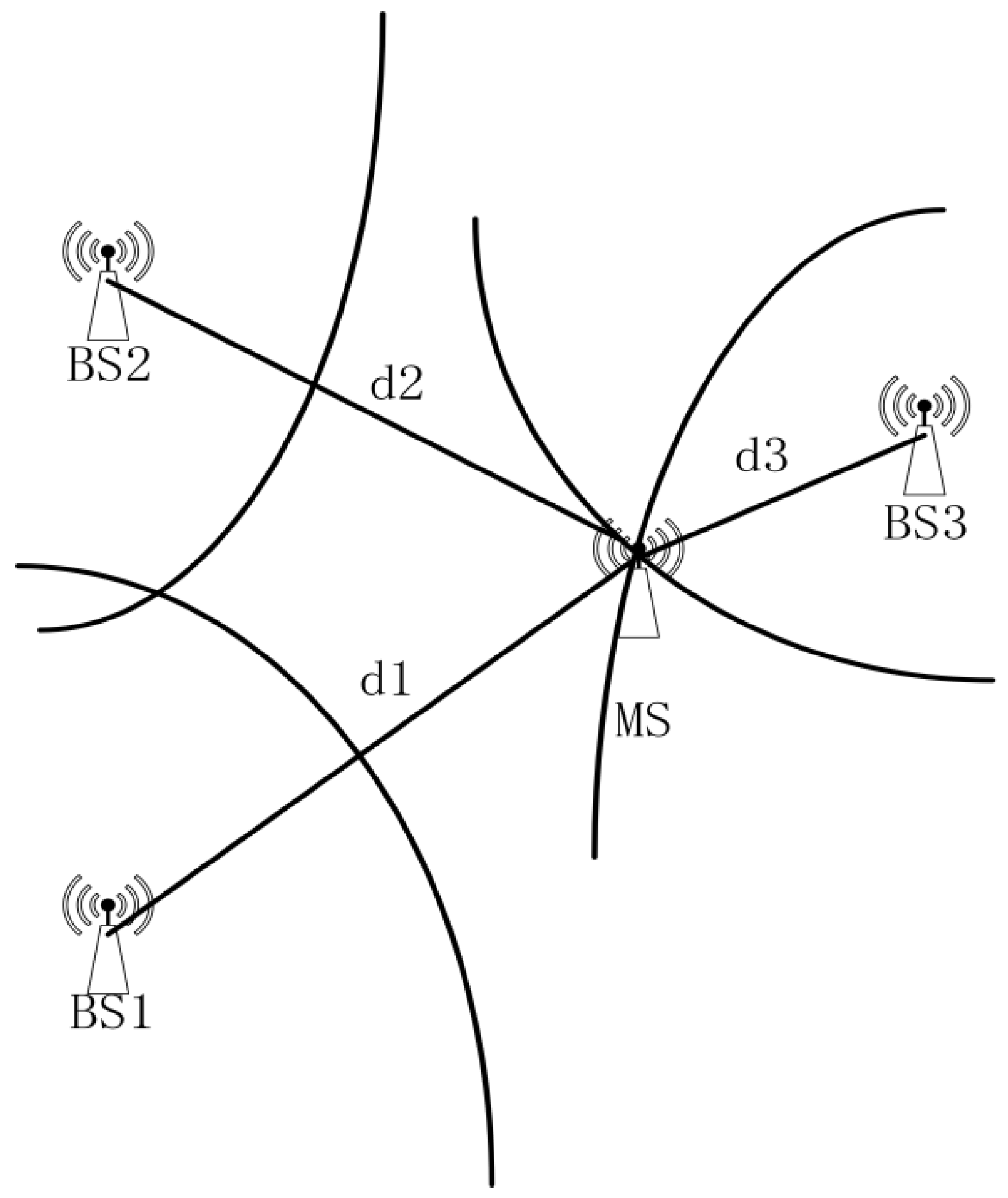
In order to achieve localization, nodes in the WSN can be divided into two types: beacon nodes and unknown nodes, where beacon nodes are also called anchor nodes or reference points, and unknown nodes are also called ordinary nodes. Beacon nodes are nodes with known location information, and unknown nodes are nodes without location information. The principle of TDOA localization is shown in Figure 1, where an unknown node broadcasts a signal to the surrounding area to anchor nodes, and the anchor nodes in the surrounding area will successively receive the signal sent by the unknown node. Then the distance difference from the unknown node to the anchor nodes can be calculated through the time difference. For example, if we know the distance difference between the unknown node MS and the anchor nodes BS1 and BS2, we know that the unknown node is on the hyperbola with BS1 and BS2 as the focal points, and similarly, MS is on the hyperbola with BS2 and BS3 as the focal points, and the coordinates of the unknown node can be determined by solving for the intersection of the hyperbolas according to some known conditions.
3.1.2. Location Model Based on Swarm Intelligence Algorithm
Taking a two-dimensional scenario as an example, we suppose there are M anchor nodes distributed on the field. The coordinates of the anchor node i and the unknown node are ,, the distance between the anchor node i and the unknown node is , and the calculation is:
We considered anchor node 1 as the main reference node, is the measured value of the distance difference between the unknown node and the anchor node i and the anchor node 1 and the unknown node. The equation is:
where is calculated as the time difference between the two anchor nodes receiving a broadcast from the unknown node and is the measurement noise. Equation (3) identifies the unknown node on a particular hyperbola, which requires at least three anchor nodes in the two-dimensional plane to unite the set of equations, and at least four anchor nodes in the three-dimensional plane, converting Equation (3) to matrix form as:
Assuming that:
where are independent Gaussian white noise random variables with zero mean and known variance of , the maximum likelihood method is used to determine the location of the unknown node (x, y). The likelihood function can be followed as:
for getting the coordinate of maximizing the likelihood function of Equation (5), it can be transformed into solving the objective function of Equation (6).
Using general methods to solve nonlinear Equation (6) will lead to high computation costs, which are very inconvenient in practical problems. After transforming Equation (6) into objective Equation (7), this paper proposes a HBES algorithm, which obtains the optimal solution for the target function by finding the individual with the highest level of adaptability.
3.2. Hybrid Bald Eagle Search Optimization Algorithm
3.2.1. Bald Eagle Search Optimization Algorithm
The bald eagle search algorithm [30] is a new metaheuristic algorithm inspired by the predatory behaviors of the bald eagle. Bald eagles use multiple attack methods to assess the energy cost of a hunting action, the energy contained in the prey, and the success rate in all kinds of habitats. They follow an intelligent strategy of selecting the correct area with prey, searching the selected area, and capturing the prey at the right time. Wise hunting strategies are also used to take advantage of wind speeds and stormy air. Bald eagle hunting behaviors involve selecting the right search area, searching the selected area, and swooping in on prey at the right time. A bald eagle usually chooses a search area that is spatially closer to the previous search area, and each of its movements is determined by the previous movements. The basic process of BES algorithm can be divided into three stages: choosing a seek space, seeking the space for prey, and diving for prey.
Step 1: Selecting a search space: The bald eagle randomly searches a large area for prey, deciding whether the area is suitable for hunting in accordance with the prey concentrative degree and its own experience. The equation for updating a bald eagle’s location is:
is for bald eagle’s own experience, which is itself is a parameter controlling position variation ranging from (1.5, 2), r is a random number between (0, 1), represents the most adapted position among individual bald eagles, represents the average position of the bald eagle population, and represents the position of the bald eagle i.
Step 2: Search space prey: The bald eagle selects a search space to search for prey and will search in and around the center point of the search space, moving in different directions within the spiral space to speed up the search, which can be expressed through the equation as:
where represents the polar angle in polar coordinates, is the polar radius in polar coordinates; a and R are parameters to govern the helix search pattern of the bald eagle, varying over the ranges (0, 5) and (0.5, 2). rand represents a random number of (0, 1), and and represent the two coordinates of the bald eagle when converted to a plane rectangular coordinate system. represents the position of bald eagle i + 1 before the population was updated.
Step 3: Swooping for prey: The bald eagle finds prey and launches a swoop toward it. The bald eagle attacks the target prey from the optimum location in the search space, and all points go to the best point. The equation for the change in position of a bald eagle is:
where c1 and c2 represent the motion intensity of the bald eagle to the optimal point and center point during the dive, and the value range is (1, 2).
3.2.2. Lévy Flight Strategy
Lévy flight has its origins in the mathematically related chaos theory [31], which is essentially a random wander with step size obeying the Lévy distribution, a power-law heavy-tailed distribution. The distribution is given by:
where w is the shape index taking values in the range (0, 2), after the research of many scholars, the foraging trajectories of many creatures fit the pattern of Lévy flight, and the swarm intelligence algorithm is also an algorithm inspired by observing the behavior of creatures. The search strategy of Lévy flight is a small step search in most cases, with occasional larger steps, and the combination with the swarm intelligence algorithm helps expand the swarm intelligence algorithm’s global search capability. The most common method currently used to solve for random step sizes is the algorithm proposed by Mentegna [32], which has been applied with good results. The formula is as follows:
where = 1.5, u and v serve the regular distribution of and , and the variance calculation method is as follows:
BES in Equation (10) is the first stage of the algorithm, the bald eagle starts a wide range of searches, laying the foundation for the subsequent search for excellence. Therefore, there is still room for improvement at this stage, combined with the Lévy flight strategy to improve the search strategy, improving the algorithm’s global search capability, and the algorithm’s search efficiency. Equation (10) is improved as follows:
3.2.3. Chaos Mapping
The initial population of BES is generated randomly, and for the D-dimensional space, the initial population is:
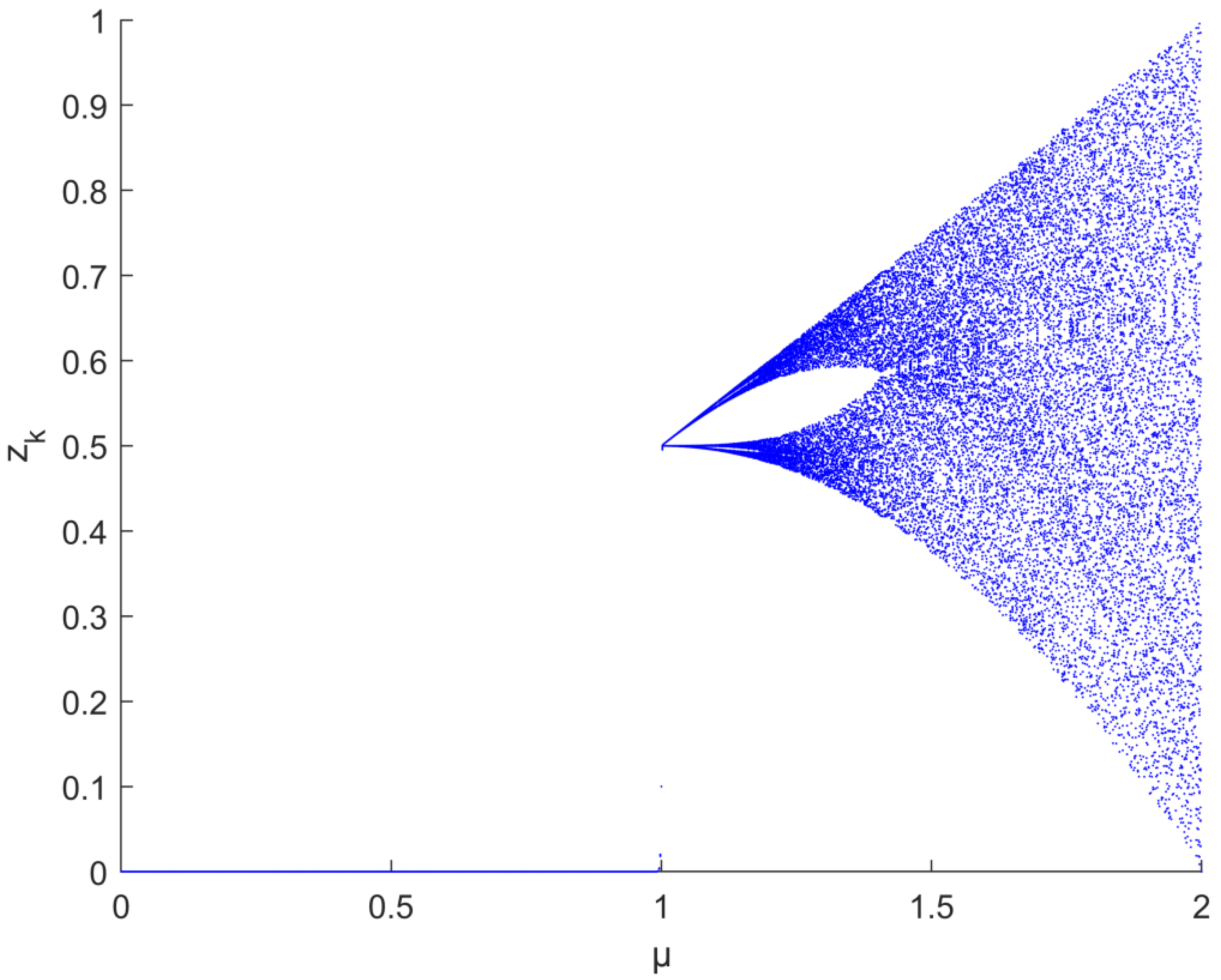
where and represent the upper and lower bounds of the population search range, represents the bald eagle i in the population, and rand is a random number of (0, 1). The initial population also has an impact on the algorithm’s capabilities in finding the optimal solution. We need the initial population to be uniformly distributed, and the wide search range of the algorithm helps to find the globally optimal solution. Chaotic mappings have been applied to swarm intelligence algorithms such as the grey wolf algorithm and whale algorithm in the literature [33,34]. Chaos mapping can increase the diversity of the initial population at the beginning of population intelligence and speed up the convergence of the algorithm. The bifurcation diagram for drawing the Tent map is shown in Figure 2. In this paper, the population expression of the tent-mapping initialized bald eagle algorithm was chosen as follows:
3.2.4. Sine Cosine Algorithm
The second phase of the BES algorithm searches for spatial prey is to search for prey in a spiral flight search based on the first phase with respect to the region selected in the first phase. This transition phase can be helpful for the algorithm to go beyond the local optimum to ultimately get the best value if it increases the search convenience and the exploration of the solution space. The sine cosine algorithm proposed by Mirjalili [35] in 2016 is characterized by fast convergence speed and few adjustment parameters. The sine cosine algorithm replaces the process of biological searching for food in the swarm intelligence algorithm by the oscillation of the sine and cosine function. The position update formula of the sine cosine algorithm is as follows:
where t is the current iteration number, represents the particle i of the t iteration, , , are random numbers whose values range is (0, 2), (−2, 2), (0, 1) respectively. represent the individual with the best fitness in the current population, and is a parameter that linearly decreases with the number of iterations and controls the switching between global search and local development of the algorithm.
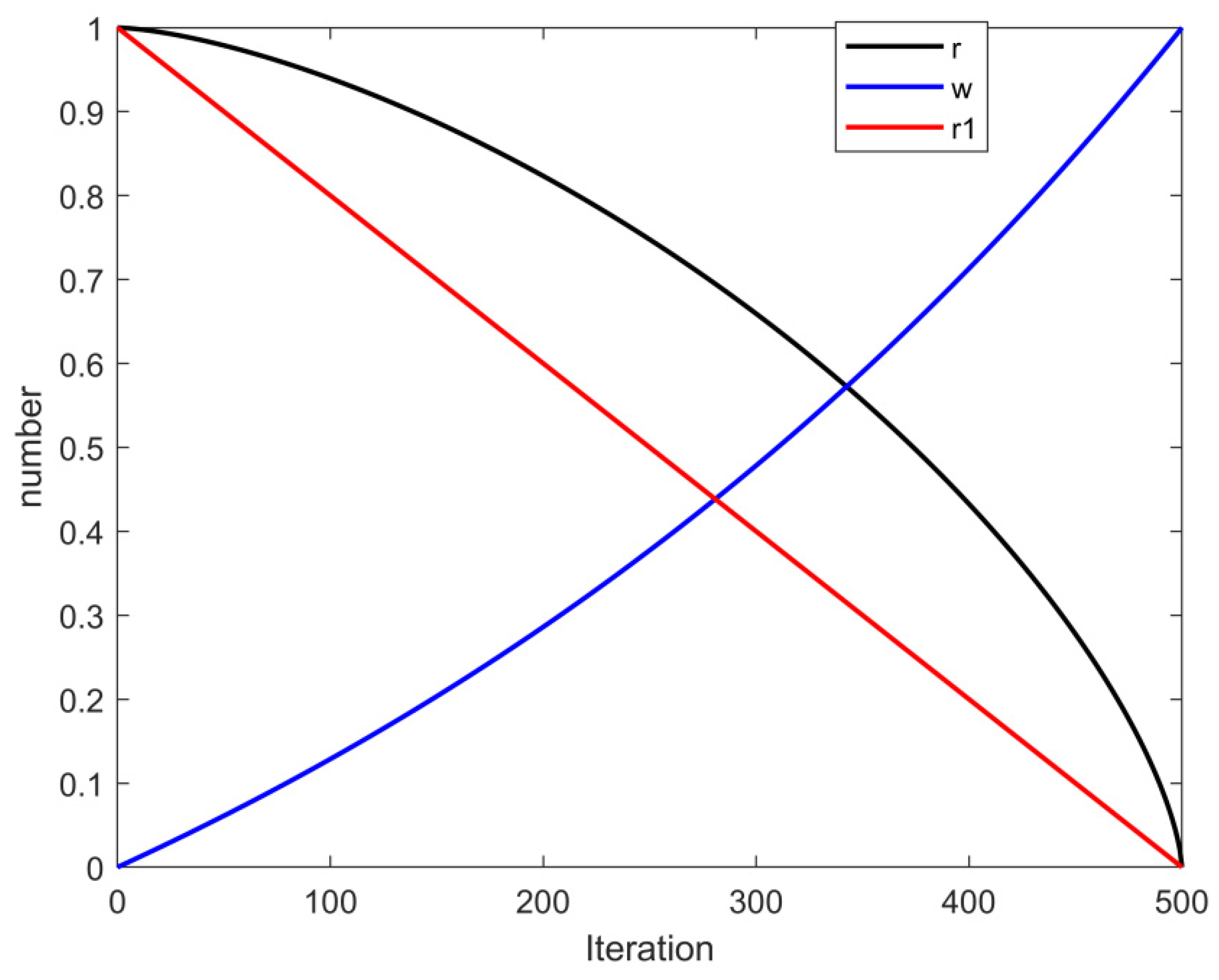
where T is the total number of iterations, when or is greater than 1 the algorithm deviates from to enhance the algorithm’s global search, when or less than or equal to 1 the algorithm is close to to facilitate the algorithm’s local exploration to find the optimal solution. This paper incorporates the oscillation mechanism of the positive cosine algorithm in the second stage of the BES algorithm to adjust the local development mode of the global search of the algorithm and improve the algorithm’s ability to find the optimal solution. Because is linearly decreasing, this paper adjusts as a nonlinear parameter to facilitate the global search in the early stage of slow decline, and local development in the late stage of fast decline to find the optimal solution, while introducing a nonlinear weight factor to adjust the dependence of the bald eagle algorithm on individual information. In order to match the conversion pattern of , is smaller in the early stage and larger in the late stage, which is in line with the strategy of global search in the early stage and local development in the late stage.
Equation (25) is the adjusted , Equation (26) is the expression of , and Equation (27) is the improved expression of the bald eagle search algorithm’s two-stage integration with the sine cosine algorithm. The curves of r, , with iteration number are shown in Figure 3.
3.2.5. Opposition-Based Learning
The opposition-based learning strategy is a mathematical method proposed by Tizhoosh [36] in 2005, which is an idea to expand the solution space by generating corresponding reverse solutions again based on the basis of the present solution space and then selecting the best solution from it for the next iteration. This strategy can be a good way to expand the population size of a swarm intelligence algorithm and extend the range of the algorithm’s superiority search. In this paper, the population size is expanded by incorporating a backward learning strategy in the closing stage of the bald eagle algorithm to further improve the algorithm’s merit-seeking ability. The population expansion formula is:
Equation (28) is the mathematical expression for generating a reverse population. ub and lb represent the upper and lower bounds of population search, respectively, and are the current population and reverse population, respectively.
3.2.6. Time Complexity Analysis
Supposing the population size of HBES is n, the dimension of the search space is d, Then the Tent mapping initialization complexity of the population is . In addition, the maximum evaluation times also influence the time complexity. The computation complexity of the fitness value is , the complexity of the three-position update is , the sorting complexity of the fitness value of the algorithm is , and the control parameter r, , updates the complexity of the algorithm is . Generating reverse populations and sorting complexity is . Then, the time complexity of HBES is:
However, the original BES algorithm has the same initialization population n, maximum evaluation times , and the dimension of search space d as the proposed HBES. The time complexity of the initialization phase is ; calculating the fitness of all agents is ; the position update is . Consequently, the time complexity of the BES algorithm is:
In summary, the time complexity of the HBES algorithm is slightly higher than that of BES algorithm for the same number of iterations. However, the optimization capability of the advanced algorithm is superior to BES, and both of them are in the same order of magnitude. Speed of optimization, optimization capability, and robustness of the proposed method can be proved in the following experiments, including the 23 benchmark functions test, and TDOA problems test, respectively.
3.3. TDOA Localization Implementation Process and Pseudo Code Based on HBES
This section applies HBES to the WSN localization scenario, solving the nonlinear equations for TDOA localization to derive the estimated coordinates of the unknown nodes. The specific steps and pseudo-code for the implementation of TDOA localization based on HBES are shown below.
Step 1: First, the modelling of TDOA localization is started by setting the number of anchor nodes and unknown nodes, randomly generating the coordinates of the anchor and unknown nodes. After that, start the localization and calculate the distance between each node based on the communication time between the nodes.
Step 2: Initialize the population using Tent mapping and configure the basic parameters of HBES algorithm such as population dimension dim, the maximum number of iterations T, population size N, population search boundary ub, lb, etc.
Step 3: Calculate the search space of the current population and return the individuals that exceed the search space.
Step 4: Calculate the fitness of each individual in the population and rank them; record the current best fitness value.
Step 5: Introduce the Lévy flight to promote the algorithm ability of global search and perform a global search of the initialized population of individuals according to Equation (20) with the HBES algorithm, after which the fitness values of the individuals in the population are ranked to complete a phase of position updating.
Step 6: Then, the search mechanism of the positive cosine algorithm is added to perform the local search of the HBES algorithm, and the spatial prey phase of the HBES algorithm is entered according to Equation (27), followed by the spiral search phase according to Equation (13).
Step 7: Finally, expand a set of reverse populations and calculate the fitness of the reverse populations, selecting the updated populations and the individuals with the highest fitness in the reverse populations.
Step 8: Repeat steps 3–7 until the number of iterations reaches a maximum or the overall extreme accuracy value meets a predetermined minimum accuracy value to obtain the optimal coordinates for the TDOA localization model. Pseudo code of HBES-based TDOA positioning process is shown in Algorithm 1.
| Algorithm 1: Pseudo code of HBES-based TDOA positioning process |
|
4. Experimental Design and Analysis
4.1. Experimental Design
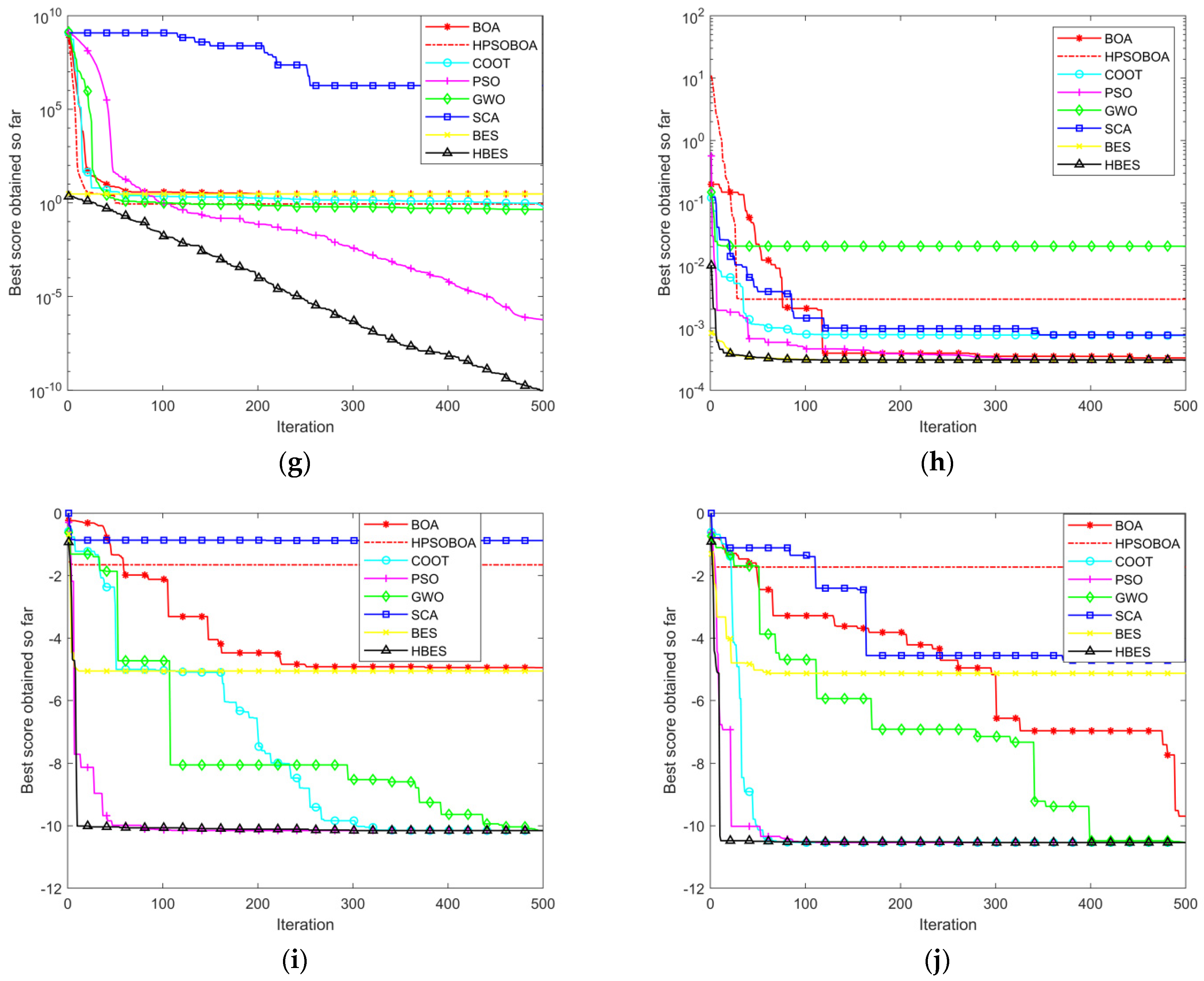
First, the HBES algorithm is compared with PSO [37], GWO [38], COOT [39], BOA [40], HPSOBOA [41], and the BES algorithms, respectively, on the benchmark test functions for finding the best result. HBES algorithm was then combined with TDOA localization and PSO, GWO, COOT, and BES for comparative analysis. The test functions are divided into three categories, single-peaked functions, multi-peaked functions, and fixed-dimensional functions. The parameters of the test function is shown in Table 1. The optimization finding accuracy was set to .
The experimental environment is Windows 10 operating system, AMD R7-5800H [email protected] GHz, 16 G memory, and MATLAB 2020A simulation platform.
Definition 1.
Optimization success rate (SR): When the difference between the optimal value and the theoretical optimal value is less than the optimization accuracy, the optimization is considered to be successful, and the success rate is the times of successful optimizations divided by the times of experiments.
4.2. Performance Evaluation
We obtained experimental data from the designed experiments and plotted the data in the form of graphs to facilitate performance analysis of the hybrid bald eagle algorithm against other algorithms.
4.2.1. Comparison of Benchmark Test Function Optimization
In order to ensure the fairness of each algorithm on the optimization search experiment, the population size of each algorithm is N = 30, where the dimensionality of the single-peaked test function and the multi-peaked function is dim = 30, the dimensionality of the fixed-dimensional function is as required by the table, and the maximum number of iterations for each algorithm is = 500. For the same test function, each population intelligence algorithm is run 50 times independently, and the mean, standard deviation (std), and the success rate (SR) are calculated based on the statistical values. The mean, standard deviation, and success rate are calculated based on the statistical values. The results of the optimization experiments are shown in Table 2.
As can be seen from Table 2, for the single-peak functions, the search results of , , and show that BES, HBES, and the HPSBOA are better than the other algorithms, and the search success rate reaches 100%, while the remaining single-peak functions of the BES and HBES algorithms are not very different. For the multi-peak functions, the HBES algorithm achieves a much better search result at , and to are all around the theoretical optimum, with being slightly better than the original algorithm. Except for , the rest of the multi-peaked functions are better with the BES and HBES. Among the fixed-dimensional functions, the HBES algorithm performs better in , and . Statistical analysis of the search results in Table 2 yields Table 3, from which it can be seen that the HBES algorithm has better combined results in terms of search accuracy and stability among the 23 tested functions, and in most cases, maintains the leading position or is tied for first place with other swarm intelligent algorithms.
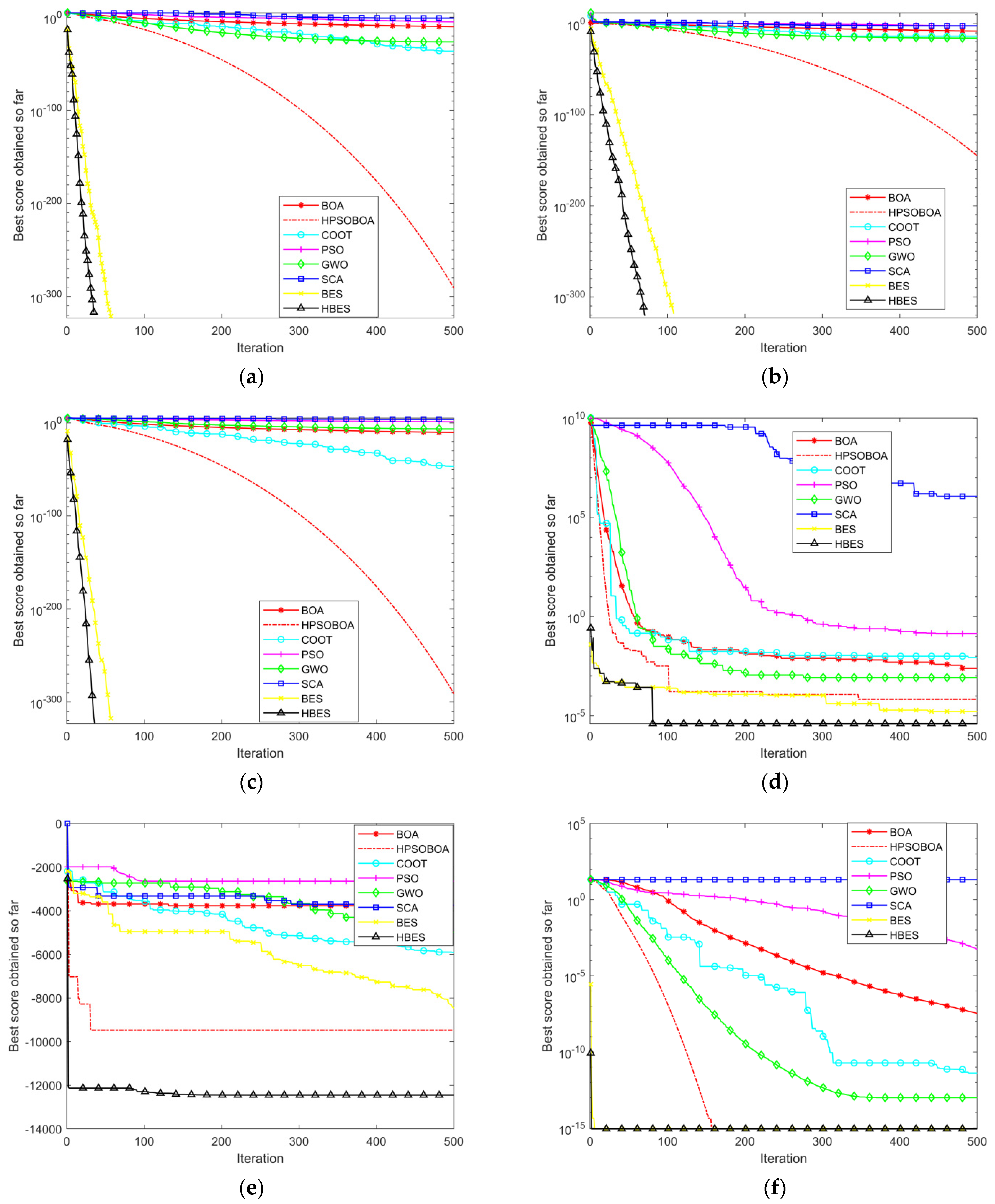
In order to further compare the convergence speed and convergence accuracy of each algorithm, the curve of the optimization seeking process of the test function is observed, as shown below.
In Figure 4, the single-peaked functions , and of the BES algorithm and HBES algorithm have the same search accuracy and converge to the theoretical optimum value of 0. However, Figure 4 shows that the convergence speed of the single-peaked functions has improved, while the performance on is still not as good as the original algorithm. In the test of the multi-peaked functions, has the biggest improvement in convergence performance and convergence accuracy, while and have a more obvious improvement in convergence speed. In the test of fixed-dimensional functions, the convergence speed and convergence accuracy of the hybrid condor algorithm have been maintained in the leading position among these algorithms.
4.2.2. HBES-Based Simulation of TDOA Localization
In order to verify the performance of the HBES algorithm for TDOA localization, the combination of the HBES algorithm and other intelligent algorithms (PSO, GWO, COOT, BES, SSA [26], CPSO [27]) are compared.
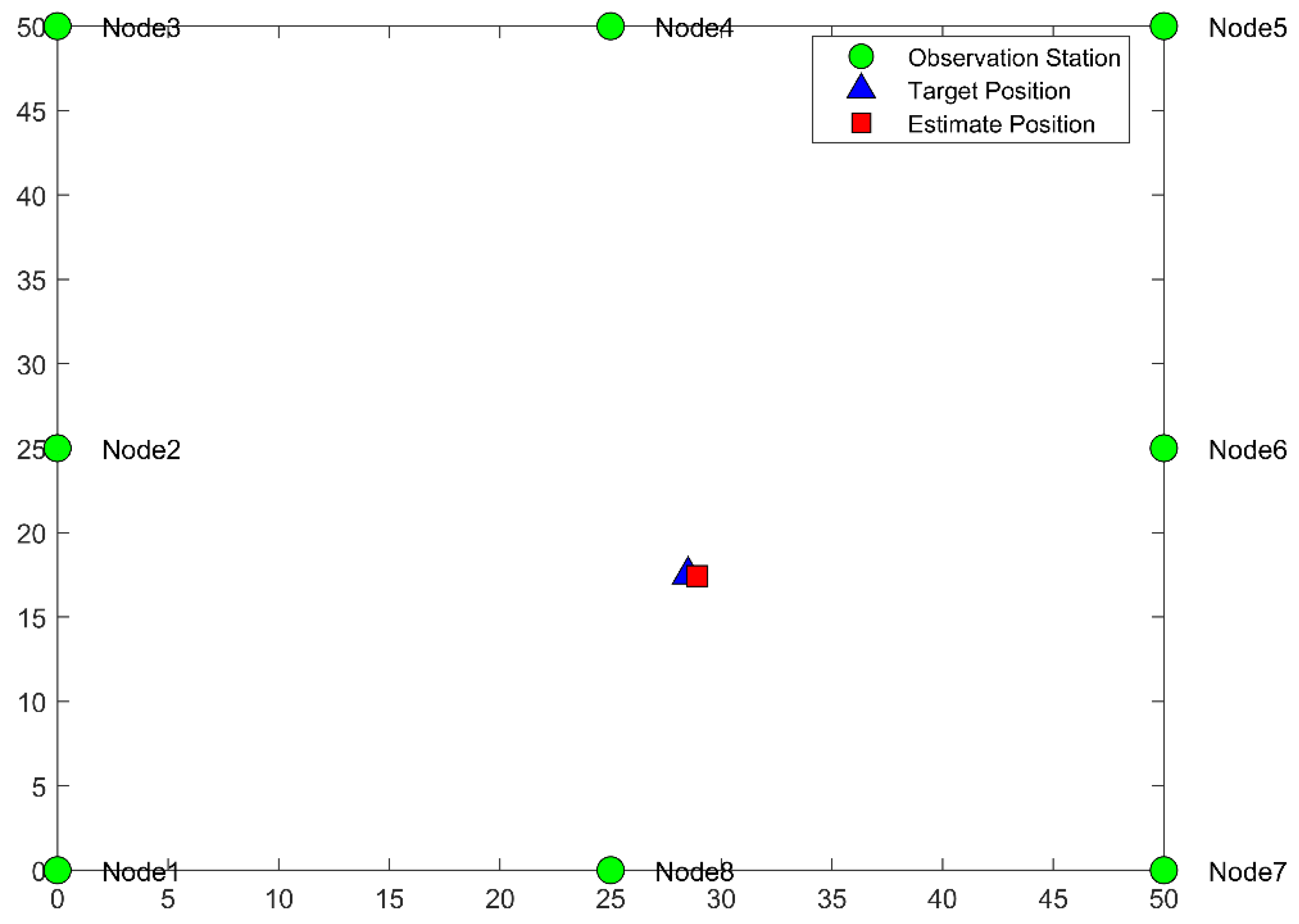
The simulation scenario and parameters are set as follows: 8 base stations are deployed in a 50 m × 50 m range with base station coordinates of (0, 0), (0, 25), (0, 50), (25, 50), (50, 50), (50, 25), (50, 0), (25, 0), the superior limit of 2D plane coordinates ub = [50, 50], the inferior limit lb = [0, 0], and the number of iterations of all swarm intelligence algorithms The Root Mean Square Error (RMSE) was selected as the evaluation index for localization accuracy.
where and are the true and estimated positions of the test point p, respectively, and P is the total number of test points. The performance of the localization algorithm is usually assessed based on whether the root mean square error is close to the Cramér–Rao Lower Bound (CRLB). The Cramér–Rao Lower Bound specifies the lower limit on the standard deviation that can be achieved by an unbiased estimator, representing the theoretical best estimation accuracy, and is calculated as:
where the trace [] function is used to find the trace of the matrix, is the standard deviation of the distance noise, and are the coordinates of the unknown node and base station I, respectively, is the distance from the unknown node to the base station, and N is the total number of base stations.
4.2.3. Analysis of the Accuracy of TDOA Positioning Based on HBES
The population size M is set to 100, the number of base stations N is set to 8, and the values of distance noise standard deviation is set at 0.2, 0.4, 0.6, 0.8, and 1.0 for the experiment, and the experimental scenario is shown in Figure 5. The comparison of the positioning accuracy for different distance noise standard deviations was obtained, as shown in Table 4. It can be seen that the noise immunity of PSO, SSA, and COOT is poor. When the noise standard deviation is 0.2, the RMSE is close to CRLB. As the noise standard deviation increases, the difference between RMSE and CRLB becomes larger. The CPSO, BES, and GWO have a good positioning accuracy in low noise conditions. The results of CPSO and PSO show that chaotic mapping can promote the optimization ability to some degree. Overall, the HBES algorithm has the best noise immunity and its RMSE is always close to that of CRLB.
The effect of the number of base stations on the localization was analyzed under the condition that the standard deviation of the distance noise was 0.5 m. Experiments were conducted with 4–8 base stations involved in localization, and the comparison of the localization accuracy with different numbers of base stations was obtained, as shown in Table 5. The RMSE and CRLB of different algorithms decrease as the number of base stations increases, and HBES algorithm achieves a lower RMSE for different numbers of base stations, which is closer to the CRLB than other algorithms when the number of base stations increases from 4 to 8, the RMSE of HBES algorithm decreases by 2.34%, 4.17%, 7.8%, 8.24%, 9.06%, and 9.06% respectively compared to the BES algorithm. This indicates that the HBES algorithm can make fuller use of the redundancy of measurement values to reduce the positioning error and can perform better in high-precision positioning scenarios with enough base stations. In general, the difference between the positioning accuracy of HBES and other algorithms is not significant when the quantity of base stations is 4. When the quantity of base stations is increased, the RMSE of HBES is lower than that of the other algorithms. This indicates that the HBES algorithm can be used for TDOA positioning with good accuracy while the quantity of base stations is appropriate and that the HBES algorithm has good stability against noise interference and can achieve good positioning accuracy in the presence of interference.
4.2.4. Analysis of the Convergence Performance of TDOA Based on HBES
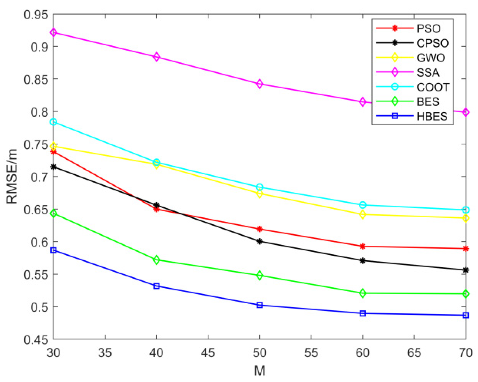
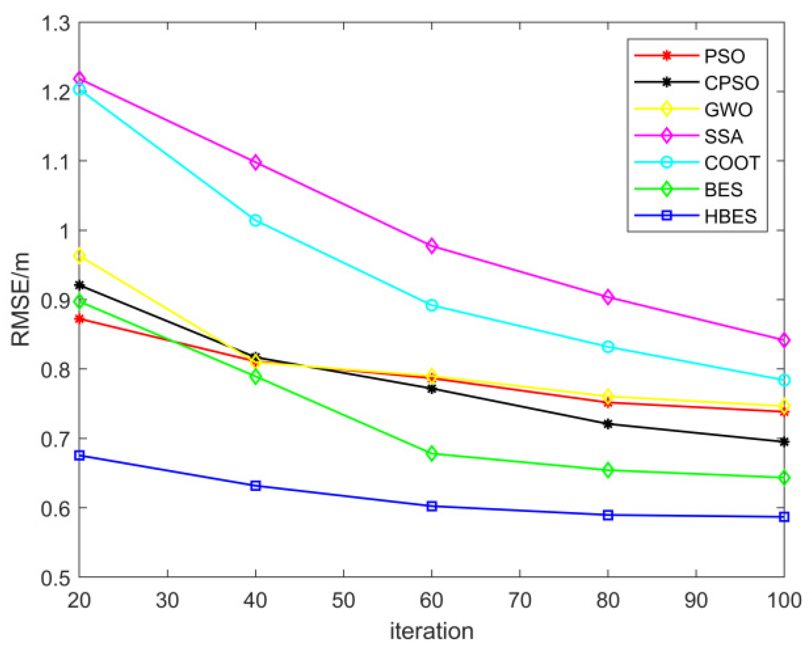
Swarm intelligent optimization algorithms require a certain population size and number of iterations to complete the search for the global optimal solution. Swarm intelligent optimization algorithms with good convergence capability can converge at smaller population sizes or fewer iterations, reducing running time. Experiments were conducted under the condition that the number of base stations was 8 and for 0.6 m varying the population size M. The relationship between RMSE and population size was obtained as shown in Figure 6. The RMSE of SSA, COOT, PSO, CPSO changes significantly with the increase in population size. the RMSE of GWO, BES no longer decreases significantly after the population size reaches 50. The RMSE of HBES tends to be stable after the population size. The RMSE of HBES stabilized after the population size reached 50. It can be seen that CPSO and HBES have better initial solutions than PSO and BES after using chaotic mapping to initialize the populations so that the individuals of the populations can quickly focus on the global optimal solution and search around it, which improves the efficiency of the search. The population size M is set to 30, and the convergence of RMSE of different algorithms was compared under the increasing number of iterations, and the relationship between RMSE and the number of iterations was obtained, as shown in Figure 7. The RMSE of SSA, COOT, and PSO has a steep decline curve, indicating that the algorithms are easily affected by the number of iterations. The HBES algorithm enhances the global search capability through opposition-based learning and Lévy flight, allowing the algorithm to find an initial value with a smaller RMSE faster and to calculate the location of the target using fewer iterations. Therefore, applying the HBES algorithm to TDOA localization can achieve smaller population sizes and iterations, and reduce the time taken to compute the results.
4.2.5. Comparison of 3D Scene Positioning
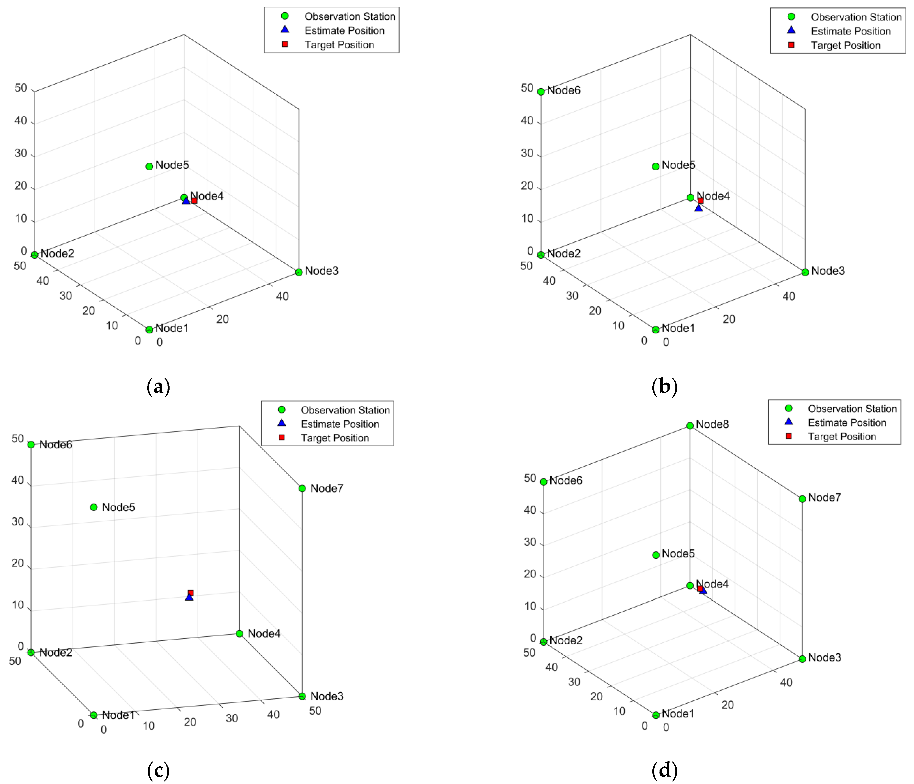
The above experiments are the application of the swarm intelligence algorithm in the two-dimensional scene, and three-dimensional space positioning is also one of the important applications of the sensor network. Therefore, TDOA localization based on HBES algorithm is applied to 3D scene. The experimental scene of this experiment is set in a three-dimensional space of 50 m × 50 m × 50 m. When the quantity of base stations was 5, 6, 7, and 8, the algorithm was independently run 50 times, and the average value and standard deviation of positioning errors of each algorithm were recorded.
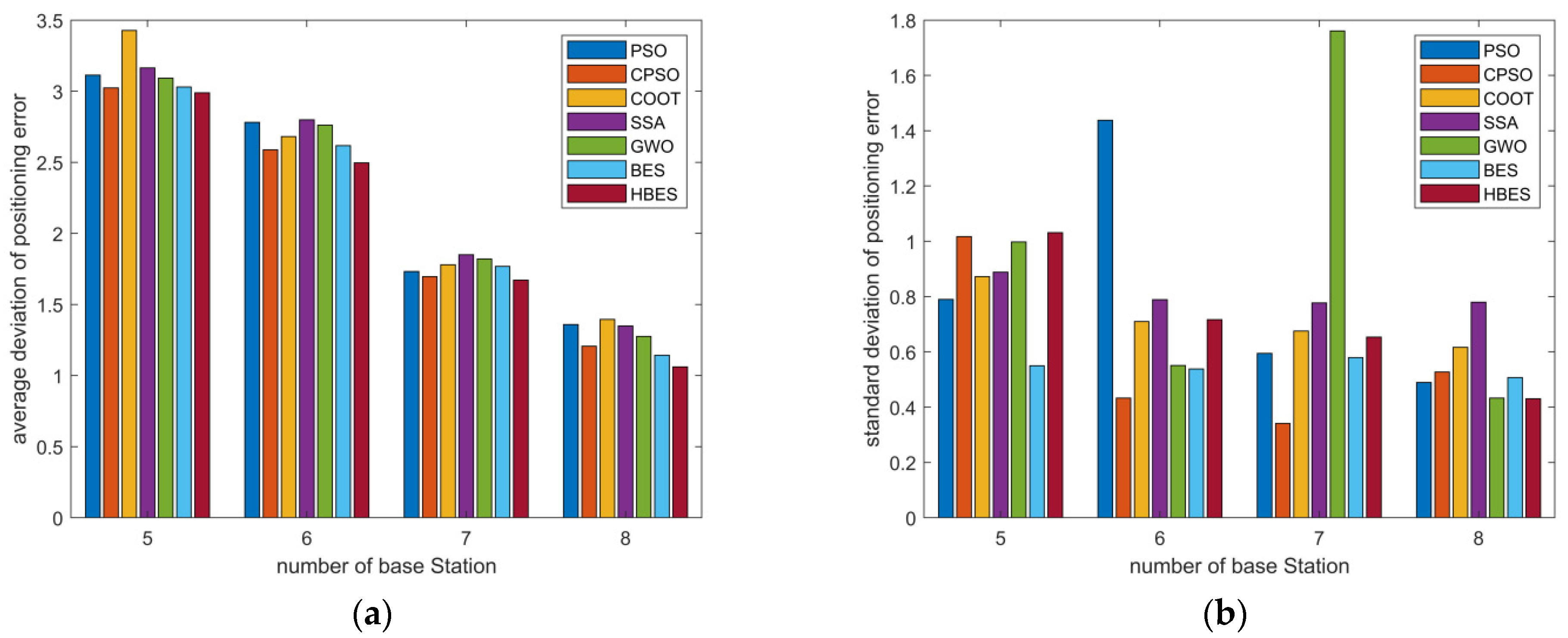
The positioning data and effects of each algorithm in 3D scenes are shown in Figure 8 and Figure 9. Figure 8 imagines the unknown and anchor nodes as points in 3D space, and the estimated locations are the locations found by the TDOA localization method based on the swarm intelligence algorithm. The closer the points of the triangle and the points of the square in the figure indicate, the better the accuracy of the localization. Figure 9 shows the histogram of the average error of the experimental simulation, which shows that the average error of all seven algorithms decreases as the number of base stations increases in the 3D scenario. The average errors of CPSO, BES, and HBES remained consistently low as the number of base stations changed. The HBES improved over the BES algorithm by 1.4%, 4.6%, 5.4%, and 7.1%, respectively, and over CPSO by 1.1%, 3.6%, 1.4%, and 11.9%, respectively, as the number of base stations increased. The standard deviation reflects the stability of the algorithm in solving the positioning coordinates. The HBES algorithm is less stable when the number of base stations is small, and the standard deviation becomes smaller as the number of base stations increases, remaining at the top of the seven algorithms while the quantity of base stations is 8. It can be seen that the TDOA positioning algorithm based on the HBES algorithm for 3D scenes has good positioning accuracy and stability compared with other algorithms, and the method is simple in model and is easy to implement.
5. Conclusions
The purpose of the research in this article is to further address the problem of poor TDOA localization accuracy by using swarm intelligence algorithms. To achieve this goal, we proposed an improved BES method named HBES algorithm and applied HBES to the TDOA problem with higher accuracy and precision than that of other similar algorithms. In the basic BES algorithm, chaotic mappings are introduced to initialize the population. A Lévy flight strategy is incorporated to expand the global search capability of the algorithm, and an opposition-based learning strategy is added to increase the ability of the algorithm to step out of local optima, which can promote the optimization-seeking accuracy and convergence speed of BES.
In order to verify the performance of HBES, firstly, we performed an experimental simulation with other advanced swarm intelligence algorithms in 23 test functions for finding the optimum. At last, in the two-dimensional and three-dimensional scenarios, we respectively analyzed the impacts of some aspects, such as noise effects, number of base stations, number of algorithm iterations, and population size on the TDOA localization. As a general conclusion, the HBES metaheuristic algorithm has better convergence accuracy and faster convergence speed in the test function experiments and shows the best performance, solution quality, and robustness in dealing with the node localization problem.
In this paper, the TDOA localization problem was not yet identified in the real scenarios. Therefore, in order to improve the practicality of this research, further research will be carried out on TDOA localization in indoor, underwater, and underground scenarios. Since many of the challenges from the research area of WSNs belong to the NP-hard optimization group and the swarm intelligence metaheuristic is proven to be a robust solution method for such problems, we will apply HBES to other problems in WSNs, such as deployment, coverage, and routing. Moreover, there are many opportunities for improvement in swarm intelligence research. We also plan to explore the existing population intelligence algorithms for improvement research to make swarm intelligence work better in the field of WSNs.
Author Contributions
Conceptualization, W.L. and J.Y.; formal analysis, W.L., T.Q. and Y.F.; investigation, F.L.; methodology, W.L. and W.W.; software, W.L.; supervision, J.Z. and J.Y.; validation, W.L.; writing—original draft, W.L.; writing—review and editing, J.Y. and J.Z.; data curation, J.Z.; funding acquisition, J.Z., W.W., T.Q., Y.F., F.L. and J.Y.; project administration, J.Y. All authors have read and agreed to the published version of the manuscript.
Funding
This research was funded by NNSF of China (No. 61640014, No. 61963009), Industrial Project of Guizhou province (No. Qiankehe Zhicheng [2022]Yiban017, [2019]2152), Innovation group of Guizhou Education Department (No. Qianjiaohe KY[2021]012), Science and Technology Fund of Guizhou Province (No. Qiankehejichu [2020]1Y266), CASE Library of IoT (KCALK201708), and the platform regarding the IoT of Guiyang National High Technology Industry Development Zone (No. 2015).
Institutional Review Board Statement
Not applicable.
Informed Consent Statement
Not applicable.
Data Availability Statement
Not applicable.
Conflicts of Interest
The authors declare no conflict of interest.
References
- Yaqoob, I.; Hashem, I.A.T.; Ahmed, A.; Kazmi, S.A.; Hong, C.S. Internet of things forensics: Recent advances, taxonomy, requirements, and open challenges. Futur. Gener. Comput. Syst. 2018, 92, 265–275. [Google Scholar] [CrossRef]
- Srinivasan, C.R.; Rajesh, B.; Saikalyan, P. A review on the different types of Internet of Things (IoT). J. Adv. Res. Dyn. Control Syst. 2019, 11, 154–158. [Google Scholar]
- Jagannath, J.; Polosky, N.; Jagannath, A. Machine learning for wireless communications in the Internet of Things: A comprehensive survey. Ad Hoc Netw. 2019, 93, 101913. [Google Scholar] [CrossRef] [Green Version]
- Malik, H.; Alam, M.M.; Pervaiz, H. Radio resource management in NB-IoT systems: Empowered by interference prediction and flexible duplexing. IEEE Netw. 2019, 34, 144–151. [Google Scholar] [CrossRef]
- KKhan, S.Z.; Malik, H.; Sarmiento, J.L.R.; Alam, M.M.; Le Moullec, Y. DORM: Narrowband IoT Development Platform and Indoor Deployment Coverage Analysis. Procedia Comput. Sci. 2019, 151, 1084–1091. [Google Scholar] [CrossRef]
- Rashid, B.; Rehmani, M.H. Applications of wireless sensor networks for urban areas: A survey. J. Netw. Comput. Appl. 2016, 60, 192–219. [Google Scholar] [CrossRef]
- Navarro, M.; Davis, T.W.; Liang, Y. ASWP: A long-term WSN deployment for environmental monitoring. In Proceedings of the 12th International Conference on Information Processing in Sensor Networks, Philadelphia, PA, USA, 8–13 April 2013; pp. 351–352. [Google Scholar]
- Chiang, S.Y.; Kan, Y.C.; Tu, Y.C. A preliminary activity recognition of WSN data on ubiquitous health care for physical therapy. In Recent Progress in Data Engineering and Internet Technology; Springer: Berlin/Heidelberg, Germany, 2013; pp. 461–467. [Google Scholar]
- Shi, L.; Wang, F.B. Range-free localization mechanism and algorithm in wireless sensor networks. Comput. Eng. Appl. 2004, 40, 127–130. [Google Scholar]
- Liu, F.; Li, X.; Wang, J.; Zhang, J. An Adaptive UWB/MEMS-IMU Complementary Kalman Filter for Indoor Location in NLOS Environment. Remote Sens. 2019, 11, 2628. [Google Scholar] [CrossRef] [Green Version]
- Xiong, H.; Chen, Z.; An, W.; Yang, B. Robust TDOA Localization Algorithm for Asynchronous Wireless Sensor Networks. Int. J. Distrib. Sens. Netw. 2015, 11, 598747. [Google Scholar] [CrossRef]
- Meyer, F.; Tesei, A.; Win, M.Z. Localization of multiple sources using time-difference of arrival measurements. In Proceedings of the 2017 IEEE International Conference on Acoustics, Speech and Signal Processing (ICASSP), New Orleans, LA, USA, 5–9 March 2017; pp. 3151–3155. [Google Scholar]
- Tomic, S.; Beko, M.; Camarinha-Matos, L.M.; Oliveira, L.B. Distributed Localization with Complemented RSS and AOA Measurements: Theory and Methods. Appl. Sci. 2019, 10, 272. [Google Scholar] [CrossRef] [Green Version]
- Mass-Sanchez, J.; Ruiz-Ibarra, E.; Gonzalez-Sanchez, A.; Espinoza-Ruiz, A.; Cortez-Gonzalez, J. Factorial Design Analysis for Localization Algorithms. Appl. Sci. 2018, 8, 2654. [Google Scholar] [CrossRef] [Green Version]
- Beni, G.; Wang, U. Swarm intelligence in cellular robotic systems. In Robots and Biological Systems: Towards a New Bionics? Springer: Berlin/Heidelberg, Germany, 1993. [Google Scholar]
- Colorni, A.; Dorigo, M.; Maniezzo, V. Distributed optimization by ant colonies. In Proceedings of the 1st European Conference on Artificial Life, Paris, France, 11–13 December 1991; pp. 134–142. [Google Scholar]
- Colorni, A.; Dorigo, M.; Maniezzo, V. An investigation of some properties of an ant algorithm. In Proceedings of the Parallel Problem Solving from Nature Conference, Brussels, Belgium, 28–30 September 1992; pp. 509–520. [Google Scholar]
- Colorni, A.; Dorigo, M.; Maniezzo, V. Ant system for job shop scheduling. Oper. Res. Stat. Comput. Sci. 1994, 34, 39–53. [Google Scholar]
- Smets, P.; Kennes, R. The transferable belief model. Artif. Intell. 1994, 66, 191–234. [Google Scholar] [CrossRef]
- Vaghefi, R.M.; Buehrer, R.M. Cooperative Joint Synchronization and Localization in Wireless Sensor Networks. IEEE Trans. Signal Process. 2015, 63, 3615–3627. [Google Scholar] [CrossRef]
- Le, T.-K.; Ono, N. Closed-Form and Near Closed-Form Solutions for TDOA-Based Joint Source and Sensor Localization. IEEE Trans. Signal Process. 2016, 65, 1207–1221. [Google Scholar] [CrossRef]
- Foy, W.H. Position-location solutions by Taylor-series estimation. IEEE Trans. Aerosp. Electron. Syst. 2007, AES-12, 187–194. [Google Scholar] [CrossRef]
- Xiaomei, Q.; Lihua, X. An efficient convex constrained weighted least squares source localization algorithm based on TDOA measurements. Signal Process. 2016, 119, 142–152. [Google Scholar]
- Jihao, Y.; Qun, W.; Shiwen, Y. A simple and accurate TDOA-AOA localization method using two stations. IEEE Signal Process. Lett. 2015, 23, 144–148. [Google Scholar]
- Kenneth, W.K.; Jun, Z. Particle swarm optimization for time-difference-of-arrival based localization. In Proceedings of the Signal Processing Conference, Poznan, Poland, 3–7 September 2007; pp. 414–417. [Google Scholar]
- Tao, C.; Mengxin, W.; Xiangsong, H. Passive time difference location based on salp swarm algorithm. J. Electron. Inf. Technol. 2018, 40, 1591–1597. [Google Scholar]
- Yue, Y.; Cao, L.; Hu, J. A novel hybrid location algorithm based on chaotic particle swarm optimization for mobile position estimatio. IEEE Access 2019, 7, 58541–58552. [Google Scholar] [CrossRef]
- Shengliang, W.; Genyou, L.; Ming, G. Application of improved adaptive genetic algorithm in TDOA localization. Syst. Eng. Electron. 2019, 41, 254–258. [Google Scholar]
- Wolpert, D.H.; Macready, W.G. No free lunch theorems for optimization. IEEE Trans. Evol. Comput. 1997, 1, 67–82. [Google Scholar] [CrossRef] [Green Version]
- Alsattar, H.A.; Zaidan, A.A.; Zaidan, B.B. Novel meta-heuristic bald eagle search optimization algorithm. Artif. Intell. Rev. 2020, 53, 2237–2264. [Google Scholar] [CrossRef]
- Yanhong, F.; Jianqin, L.; Yizhao, H. Dynamic population firefly algorithm based on chaos theory. Comput. Appl. 2013, 33, 796–799. [Google Scholar]
- Leccardi, M. Comparison of three algorithms for Levy noise generation. In Proceedings of the fifth EUROMECH Nonlinear Dynamics Conference, Eindhoven, The Netherlands, 7–12 August 2005. [Google Scholar]
- Jiakui, Z.; Lijie, C.; Qing, G. Grey Wolf optimization algorithm based on Tent chaotic sequence. Microelectron. Comput. 2018, 3, 11–16. [Google Scholar]
- Chunmei, T.; Guobin, C.; Chao, L. Research on chaotic feedback adaptive whale optimization algorithm. Stat. Decis. Mak. 2019, 35, 17–20. [Google Scholar]
- Mirjalili, S. SCA: A sine cosine algorithm for solving optimization problems. Knowl.-Based Syst. 2016, 96, 120–133. [Google Scholar] [CrossRef]
- Tizhoosh, H.R. Opposition-based learning: A new scheme for machine intelligence. In Proceedings of the International Conference on Computational Intelligence for Modelling, Control and Automation and International Conference on Intelligent Agents, Web Technologies and Internet Commerce (CIMCA-IAWTIC’06), Vienna, Austria, 28–30 November 2005; pp. 695–701. [Google Scholar]
- Shi, Y.; Eberhart, R. A Modified Particle Swarm Optimizer. In Proceedings of the 1998 IEEE International Conference on Evolutionary Computation Proceedings, Anchorage, UK, 4–9 May 1998; pp. 69–73. [Google Scholar]
- Mirjalili, S.; Mirjalili, S.M. Lewis A. Grey wolf optimizer. Adv. Eng. Softw. 2014, 69, 46–61. [Google Scholar] [CrossRef] [Green Version]
- Naruei, I.; Keynia, F. A new optimization method based on COOT bird natural life model. Expert Syst. Appl. 2021, 183, 115352. [Google Scholar] [CrossRef]
- Arora, S.; Singh, S. Butterfly optimization algorithm: A novel approach for global optimization. Soft Comput. 2019, 23, 715–734. [Google Scholar] [CrossRef]
- Mengjian, Z.; Daoyin, L.; Tao, Q.; Jing, Y. A Chaotic Hybrid Butterfly Optimization Algorithm with Particle Swarm Optimization for High-Dimensional Optimization Problems. Symmetry 2020, 12, 1800. [Google Scholar]
Figure 1.
TDOA positioning principle.

Figure 2.
Tent-Mapping Bifurcation Chart.

Figure 3.
Variation curves of r, ,

Figure 4.
Simulation diagram of the test function: (a) comparison of convergence curves on ; (b) comparison of convergence curves on ; (c) comparison of convergence curves on ; (d) comparison of convergence curves on ; (e) comparison of convergence curves on ; (f) comparison of convergence curves on ; (g) comparison of convergence curves on ; (h) comparison of convergence curves on ; (i) comparison of convergence curves on ; (j) comparison of convergence curves on .


Figure 5.
Positioning accuracy-test simulation diagram.

Figure 6.
Relationship between RMSE and population size.

Figure 7.
Relationship between RMSE and iteration times.

Figure 8.
3D-scene positioning diagram: (a) 3D five-base stations; (b) 3D six-base stations; (c) 3D seven-base stations; (d) 3D eight-base stations.
Figure 8.
3D-scene positioning diagram: (a) 3D five-base stations; (b) 3D six-base stations; (c) 3D seven-base stations; (d) 3D eight-base stations.

Figure 9.
Error statistics of base stations in 3D scenes. (a) The average error of the algorithm in the experiment in different base stations; (b) the standard deviation of the algorithm in the experiment in different base stations.
Figure 9.
Error statistics of base stations in 3D scenes. (a) The average error of the algorithm in the experiment in different base stations; (b) the standard deviation of the algorithm in the experiment in different base stations.


Table 1.
Test function parameters.
| Function Classification | Test Functions | Dimension | Range of Values | Optimum Value |
|---|---|---|---|---|
| single-peaked functions | 30 | [−100, 100] | 0 | |
| 30 | [−10, 10] | 0 | ||
| 30 | [−100, 100] | 0 | ||
| 30 | [−100, 100] | 0 | ||
| 30 | [−30, 30] | 0 | ||
| 30 | [−100, 100] | 0 | ||
| 30 | [−128, 128] | 0 | ||
| multi-peaked functions | 30 | [−500, 500] | −418 × n | |
| 30 | [−5.12, 5.12] | 0 | ||
| 30 | [−32, 32] | 0 | ||
| 30 | [−600, 600] | 0 | ||
| 30 | [−50, 50] | 0 | ||
| 30 | [−50, 50] | 0 | ||
| 2 | [−65, 65] | 1 | ||
| fixed-dimensional functions | 4 | [−5, 5] | 0.0003 | |
| 2 | [−5, 5] | −1.0316 | ||
| 2 | [−5, 5] | 0.398 | ||
| 2 | [−2, 2] | 3 | ||
| 2 | [1, 3] | −3.86 | ||
| 6 | [0, 1] | −3.32 | ||
| 4 | [0, 10] | −10.1532 | ||
| 4 | [0, 10] | −10.4028 | ||
| 4 | [0, 10] | −10.5363 |
Table 2.
Comparison of algorithm search results.
| Test Function | Indicators | PSO | BOA | HPSOBOA | SCA | GWO | COOT | BES | HBES |
|---|---|---|---|---|---|---|---|---|---|
| mean | 1.15 × 10⁻⁵ | 7.71 × 10⁻¹¹ | 1.862 × 10−290 | 23.2423 | 1.25 × 10⁻²⁷ | 2.07 × 10⁻¹³ | 0 | 0 | |
| std | 2.57 × 10⁻⁵ | 6.71 × 10⁻¹² | 0 | 68.9556 | 2.1 × 10⁻²⁷ | 1.47 × 10⁻¹² | 0 | 0 | |
| SR(%) | 0 | 0 | 100 | 0 | 0 | 76 | 100 | 100 | |
| mean | 0.0063 | 2.33 × 10⁻⁸ | 8.62 × 10−146 | 0.0306 | 1.07 × 10⁻¹⁶ | 4.05 × 10⁻⁸ | 0 | 0 | |
| std | 0.0124 | 6.46 × 10⁻⁹ | 5.59 × 10−146 | 0.0439 | 8.79 × 10⁻¹⁷ | 2.86 × 10⁻⁷ | 0 | 0 | |
| SR(%) | 0 | 0 | 100 | 0 | 0 | 0 | 100 | 100 | |
| mean | 0.4956 | 6.2 × 10⁻¹¹ | 1.096 × 10−289 | 92.85 | 7.28 × 10⁻⁷ | 2.02 × 10⁻¹⁰ | 0 | 0 | |
| std | 0.2497 | 7.91 × 10⁻¹² | 0 | 53.39 | 8.65 × 10⁻⁷ | 1.39 × 10⁻⁹ | 0 | 0 | |
| SR(%) | 0 | 0 | 100 | 0 | 0 | 0 | 100 | 100 | |
| mean | 0.5364 | 3.38 × 10⁻⁸ | 2.52 × 10−146 | 34.6610 | 8.15 × 10⁻⁷ | 4.04 × 10⁻¹³ | 0 | 0 | |
| std | 0.4226 | 3.38 × 10⁻⁹ | 1.2 × 10−147 | 11.1013 | 9.05 × 10⁻⁷ | 2.66 × 10⁻¹⁶ | 0 | 0 | |
| SR(%) | 0 | 0 | 100 | 0 | 0 | 0 | 100 | 100 | |
| mean | 42.62 | 28.9069 | 28.776 | 953.3394 | 27.2613 | 44.97 | 19.0639 | 20.4183 | |
| std | 26.64 | 0.0263 | 0.0644 | 3.37 × 10³ | 0.7647 | 44.44 | 1.4906 | 0.2718 | |
| SR(%) | 0 | 0 | 0 | 0 | 0 | 0 | 0 | 0 | |
| mean | 1.15 × 10⁻⁶ | 5.4064 | 0.0416 | 40.6717 | 0.6766 | 0.2605 | 1.34 × 10⁻¹⁸ | 2.13 × 10⁻¹⁸ | |
| std | 2.04 × 10⁻⁵ | 0.5654 | 0.0318 | 166.8152 | 0.3671 | 0.2008 | 4.29 × 10⁻¹⁸ | 5.05 × 10⁻¹⁸ | |
| SR(%) | 0 | 0 | 0 | 0 | 0 | 0 | 0 | 0 | |
| mean | 0.0832 | 0.0019 | 2.14 × 10⁻⁵ | 112.9 | 0.0022 | 0.0055 | 3.98 × 10⁻⁵ | 2.47 × 10⁻⁴ | |
| std | 0.0377 | 6.81 × 10⁻⁴ | 1.05 × 10⁻⁴ | 248.6 | 0.0013 | 0.0045 | 3.77 × 10⁻⁵ | 0.0012 | |
| SR(%) | 0 | 0 | 0 | 0 | 0 | 0 | 0 | 0 | |
| mean | −2.79 × 10³ | −4.04 × 10³ | −9.745 × 10³ | −3.73 × 10³ | −5.97 × 10³ | −7.44 × 10³ | −7.48 × 10³ | −1.24 × 10⁴ | |
| std | 406.595 | 343.2 | 1.367 × 10³ | 308.97 | 840.6115 | 1.05 × 10³ | 1.60 × 10³ | 1.09 × 10³ | |
| SR(%) | 0 | 0 | 0 | 0 | 0 | 0 | 0 | 78 | |
| mean | 45.8288 | 32.8474 | 0.0643 | 38.6612 | 2.5001 | 1.04 × 10⁻¹² | 0 | 0 | |
| std | 14.4283 | 69.8399 | 0.1818 | 34.3327 | 3.299 | 6.67 × 10⁻¹² | 0 | 0 | |
| SR(%) | 0 | 0 | 0 | 0 | 0 | 84 | 100 | 100 | |
| mean | 0.0012 | 2.78 × 10⁻⁸ | 8.88 × 10⁻¹⁶ | 14.1827 | 1.05 × 10⁻¹³ | 8.39 × 10⁻¹³ | 8.88 × 10⁻¹⁶ | 8.88 × 10⁻¹⁶ | |
| std | 5.68 × 10⁻⁴ | 5.61 × 10⁻⁹ | 0 | 8.9091 | 1.85 × 10⁻¹⁴ | 5.1 × 10⁻¹² | 0 | 0 | |
| SR(%) | 0 | 0 | 0 | 0 | 0 | 0 | 0 | 0 | |
| mean | 43.0227 | 1.18 × 10⁻¹¹ | 0 | 0.9740 | 0.0028 | 2.4 × 10⁻¹¹ | 0 | 0 | |
| std | 6.8557 | 1.06 × 10⁻¹¹ | 0 | 0.4335 | 0.0066 | 1.7 × 10⁻¹⁰ | 0 | 0 | |
| SR(%) | 0 | 0 | 100 | 0 | 0 | 72 | 100 | 100 | |
| mean | 0.7678 | 0.4866 | 0.0019 | 1.06 × 10³ | 0.0398 | 0.2583 | 5.79 × 10⁻²⁰ | 5.18 × 10⁻²⁰ | |
| std | 0.6487 | 0.1274 | 0.0014 | 5.83 × 10³ | 0.0170 | 0.6319 | 3.68 × 10⁻¹⁹ | 1.02 × 10⁻¹⁸ | |
| SR(%) | 0 | 0 | 0 | 0 | 0 | 0 | 0 | 0 | |
| mean | 0.0015 | 2.777 | 0.911 | 788.27 | 0.6138 | 0.4766 | 2.8705 | 0.0059 | |
| std | 0.0044 | 0.2658 | 0.7025 | 180.74 | 0.2386 | 0.4419 | 0.4485 | 0.0144 | |
| SR(%) | 0 | 0 | 0 | 0 | 0 | 0 | 0 | 0 | |
| mean | 1.5131 | 1.1505 | 3.1745 | 1.9508 | 4.2161 | 0.9980 | 5.3268 | 2.5651 | |
| std | 1.1153 | 0.3856 | 2.7582 | 1.0009 | 3.7155 | 2.3 × 10⁻¹³ | 5.2344 | 3.2754 | |
| SR(%) | 0 | 0 | 0 | 0 | 0 | 0 | 0 | 0 | |
| mean | 5.85 × 10⁻⁴ | 3.72 × 10⁻⁴ | 0.0015 | 0.0011 | 0.0044 | 7.02 × 10⁻⁴ | 3.68 × 10⁻⁴ | 3.07 × 10⁻⁴ | |
| std | 4.37 × 10⁻⁴ | 5.26 × 10⁻⁵ | 7.9276 × 10⁻⁴ | 3.807 × 10⁻⁴ | 0.008 | 2.59 × 10⁻⁴ | 2.22 × 10⁻⁴ | 3.42 × 10⁻⁸ | |
| SR(%) | 0 | 0 | 0 | 0 | 0 | 0 | 0 | 0 | |
| mean | −1.0316 | −1.0316 | −0.6435 | −1.0316 | −1.0316 | −1.0316 | −1.0316 | −1.0316 | |
| std | 2.61 × 10⁻¹⁶ | 5.6 × 10⁻⁵ | 0.0972 | 6.1034 × 10⁻⁵ | 2.14 × 10⁻⁸ | 3.31 × 10⁻¹² | 1.48 × 10⁻⁷ | 1.53 × 10⁻⁹ | |
| SR(%) | 100 | 64 | 0 | 78 | 100 | 100 | 100 | 100 | |
| mean | 0.3979 | 0.4514 | 0.3979 | 0.4010 | 0.3979 | 0.3979 | 0.3979 | 0.3979 | |
| std | 0 | 0.0078 | 4.39 × 10⁻⁶ | 0.0032 | 3.79 × 10⁻⁶ | 0.0012 | 4.71 × 10⁻⁷ | 2.28 × 10⁻⁸ | |
| SR(%) | 0 | 0 | 0 | 0 | 0 | 0 | 0 | 0 | |
| mean | 3 | 3.5621 | 28.0966 | 3.0002 | 3 | 3 | 3 | 3 | |
| std | 1.37 × 10⁻¹⁵ | 3..6640 | 5.8650 | 3.02 × 10⁻⁴ | 3.74 × 10⁻⁵ | 1.83 × 10⁻¹² | 6.085 × 10⁻¹⁶ | 7.4587 × 10⁻¹⁸ | |
| SR(%) | 100 | 0 | 0 | 0 | 92 | 100 | 100 | 100 | |
| mean | −3.8628 | −3.8568 | −3.1973 | −3.8543 | −3.8615 | −3.8628 | −3.8628 | −3.8628 | |
| std | 1.3 × 10⁻¹⁵ | 0.0089 | 0.0094 | 0.0027 | 0.0023 | 1.89 × 10⁻¹¹ | 1.34 × 10⁻¹⁵ | 2.34 × 10⁻¹⁵ | |
| SR(%) | 0 | 0 | 0 | 0 | 0 | 0 | 0 | 0 | |
| mean | −3.2649 | −3.0238 | −2.0792 | −2.8994 | −3.2738 | −3.2958 | −3.2602 | −3.2673 | |
| std | 0.06 | 0.1649 | 8.97 × 10⁻¹⁶ | 0.3445 | 0.0675 | 0.0498 | 0.06 | 0.04 | |
| SR(%) | 0 | 0 | 0 | 0 | 0 | 0 | 0 | 0 | |
| mean | −5.4891 | −6.9961 | −1.6612 | −2.4205 | −9.3193 | −9.0522 | −7.505 | −10.1513 | |
| std | 3.2346 | 1.7411 | 0.0272 | 1.9668 | 1.9313 | 2.5766 | 2.5702 | 3.48 × 10⁻⁵ | |
| SR(%) | 32 | 0 | 0 | 0 | 0 | 78 | 48 | 94 | |
| mean | −7.1406 | −7.4507 | −1.6867 | −3.5481 | −10.0364 | −9.4728 | −7.5917 | −10.2694 | |
| std | 3.6318 | 1.6058 | 0.006 | 1.7069 | 1.4839 | 2.3699 | 2.7382 | 0.94 | |
| SR(%) | 0 | 0 | 0 | 0 | 0 | 0 | 0 | 0 | |
| mean | −5.9766 | −8.0935 | −1.7266 | −3.9590 | −10.2949 | −10.0932 | −8.1434 | −10.4024 | |
| std | 3.5971 | 1.383 | 0.004 | 1.6797 | 0.7514 | 1.5173 | 2.6336 | 1.90 × 10⁻⁵ | |
| SR(%) | 64 | 6 | 0 | 0 | 4 | 88 | 44 | 94 |
Table 3.
Comparison results of benchmark functions.
| PSO | BOA | HPSOBOA | SCA | GWO | COOT | BES | HBES | |
|---|---|---|---|---|---|---|---|---|
| Mean/+/−/= | 1/19/3 | 0/21/2 | 0/16/7 | 0/22/1 | 1/18/4 | 2/18/3 | 1/8/14 | 4/5/14 |
| Std/+/−/= | 3/19/1 | 3/13/7 | 1/22/0 | 0/13/10 | 1/22/0 | 0/12/11 | 0/12/11 | 4/9/10 |
| Total/+/−/= | 4/38/4 | 3/34/9 | 1/38/7 | 0/35/11 | 1/40/4 | 2/30/14 | 1/20/25 | 8/14/24 |
Table 4.
Localization accuracy comparison of different distance noise standard deviation.
| Location Accuracy | PSO | GWO | COOT | CPSO | SSA | BES | HBES | CRLB | |
|---|---|---|---|---|---|---|---|---|---|
| RMSE/m | 1.0 | 1.0532 | 1.0297 | 0.9966 | 1.1256 | 1.1616 | 0.8515 | 0.8396 | 0.7149 |
| 0.8 | 0.9063 | 0.9486 | 0.8845 | 0.9002 | 1.0776 | 0.7443 | 0.6543 | 0.5719 | |
| 0.6 | 0.7384 | 0.7465 | 0.7840 | 0.7150 | 0.9215 | 0.6435 | 0.5869 | 0.4289 | |
| 0.4 | 0.5133 | 0.4481 | 0.5136 | 0.4563 | 0.6512 | 0.4414 | 0.3385 | 0.2861 | |
| 0.2 | 0.1698 | 0.1921 | 0.1836 | 0.1509 | 0.2463 | 0.1856 | 0.1456 | 0.1438 |
Table 5.
Localization accuracy comparison of a different number of base stations.
| Location Accuracy | PSO | GWO | COOT | CPSO | SSA | BES | HBES | CRLB | |
|---|---|---|---|---|---|---|---|---|---|
| RMSE/m | 4 | 3.9277 | 3.7517 | 4.0423 | 3.8522 | 3.8588 | 4.0328 | 3.9384 | 1.0084 |
| 5 | 2.0468 | 1.9646 | 1.9649 | 1.8189 | 2.1965 | 1.9989 | 1.9539 | 0.9451 | |
| 6 | 1.7577 | 1.5178 | 1.7455 | 1.7175 | 1.8377 | 1.5985 | 1.4638 | 0.8799 | |
| 7 | 1.0027 | 1.0496 | 1.2084 | 1.1186 | 1.1047 | 0.9055 | 0.8767 | 0.8187 | |
| 8 | 1.0532 | 1.0297 | 0.9966 | 1.0111 | 1.0742 | 0.8515 | 0.8396 | 0.7149 |
Publisher’s Note: MDPI stays neutral with regard to jurisdictional claims in published maps and institutional affiliations. |
© 2022 by the authors. Licensee MDPI, Basel, Switzerland. This article is an open access article distributed under the terms and conditions of the Creative Commons Attribution (CC BY) license (https://creativecommons.org/licenses/by/4.0/).
Share and Cite
MDPI and ACS Style
Liu, W.; Zhang, J.; Wei, W.; Qin, T.; Fan, Y.; Long, F.; Yang, J. A Hybrid Bald Eagle Search Algorithm for Time Difference of Arrival Localization. Appl. Sci. 2022, 12, 5221. https://0-doi-org.brum.beds.ac.uk/10.3390/app12105221
AMA Style
Liu W, Zhang J, Wei W, Qin T, Fan Y, Long F, Yang J. A Hybrid Bald Eagle Search Algorithm for Time Difference of Arrival Localization. Applied Sciences. 2022; 12(10):5221. https://0-doi-org.brum.beds.ac.uk/10.3390/app12105221
Chicago/Turabian StyleLiu, Weili, Jing Zhang, Wei Wei, Tao Qin, Yuanchen Fan, Fei Long, and Jing Yang. 2022. "A Hybrid Bald Eagle Search Algorithm for Time Difference of Arrival Localization" Applied Sciences 12, no. 10: 5221. https://0-doi-org.brum.beds.ac.uk/10.3390/app12105221
Note that from the first issue of 2016, this journal uses article numbers instead of page numbers. See further details here.