Design and Calibration of Moisture Sensor Based on Electromagnetic Field Measurement for Irrigation Monitoring

Abstract

Soil moisture control is crucial to assess irrigation efficiency in green areas and agriculture. In this paper, we propose the design and calibration of a sensor based on inductive coils and electromagnetic fields. The proposed prototypes should meet a series of requirements such as low power consumption, low relative error, and a high voltage difference between the minimum and maximum moisture. We tested different prototypes based on two copper coils divided into two different sets (P1–P15 and NP1–NP4). The prototypes have different characteristics: variations in the number and distribution of spires, existence or absence of casing, and copper wires with a diameter of 0.4 or 0.6 mm. In the first set of experiments carried out in commercial soil, the results showed that the best prototypes were P5, P8, and P9. These prototypes were used in different types of soils, and P8 was selected for the subsequent tests. We carried the second set of experiments using soil from an agricultural field. Based on the data gathered, mathematical models for the calibration of prototypes were obtained and verified. In some cases, two equations were used for different moisture intervals in a single prototype. According to the verification results, NP2 is the best prototype for monitoring the moisture in agricultural lands. It presented a difference in induced voltage of 1.8 V, at 500 kHz, between wet and dry soil with a maximum voltage of 5.12 V. The verification of the calibration determined that the calibration using two mathematical models offers better results, with an average absolute error of 2.1% of moisture.

1. Introduction

Ensuring the correct irrigation of agricultural fields and green areas is a significant problem in several countries. The problematic worsens in countries with semi-arid and arid environments, characterized by high evapotranspiration of fields and low water availability [1]. Effects of water scarcity on crop irrigation are already considered a problem for the population of many countries [2]. Considering this scenario, tailored irrigation management is essential to ensure the correct distribution of water resources along with the different areas and different uses. On the one hand, irrigation of agricultural fields ensures the production of high-quality products. On the other hand, recreational lawns in urban areas require irrigation to maintain the grass quality. This problem is aggravated when the soil’s moisture needs are unknown, and water is wasted due to the deficient irrigation system [3]. Therefore, monitoring the soil moisture in the different irrigated areas is the first step for properly integrated water management plans.

To understand the relationship of water to the vegetation and soil it supports, two parameters must be considered, the Field Capacity (FC) and the Wilting Point (WP) [4]. FC determines the capacity of the soil to keep the water, and WP is the minimum moisture at which a plant can no longer extract water from the soil. The ideal amount of water for plant growth is located between FC and WP. FC varies depending on soil texture, being higher for clay soils (40% soil moisture) and lower for sandy soils (20% soil moisture) [5]. In soils with an abundance of clay and silt, the WP usually reaches 24%, being 7% in sandy soils [5].

With the increase in water scarcity, new technologies to monitor the environment are crucial to prevent water waste. Internet of Things (IoT) is a valuable tool that can be applied to optimize irrigation. IoT has demonstrated optimal performance in new progressive urban models [6] and agriculture [7,8]. Nowadays, automatization has been incorporated in some crops and green areas to obtain the highest irrigation efficiency without human interaction [9,10,11,12]. Smart sprinklers adapt watering depending on weather, crop, and soil conditions. There are methods to determine sensor coverage for better estimating water demand [13]. The use of Autonomous Aerial Vehicles with built-in color sensors is one of the current solutions capable of determining vegetation cover in gardens [14]. Determining the plant coverage is important to ensure adequate irrigation and reduce the system’s energy consumption [15]. One solution to this is implementing a model based on real-time feedback, which lets the irrigation adapt to external disturbances [16].

Some moisture sensors are becoming commercially available. Adeyemi et al. [17] tested three different commercial sensors (Hydraprobe II, GS1, TDR 315). All of them used Maxwell’s equation to calculate the dielectric permittivity. Dielectric permittivity is related to the volume of water in the soil. In another work, Costa et al. [18] tested the design and fabrication of self-powered capacitance sensors, which could be installed in the sprinklers. Monitoring the soil moisture allows for the optimization of irrigation, thus improving the use of water resources. Wireless Sensor Networks (WSNs) are being used for managing water resources of urban lawns and agriculture [19,20]. There is no doubt of the benefits of using WSN for urban areas [21]. Current solutions for soil moisture monitoring present the same problem—the sensor must be in direct contact with the ground. To solve this problem, we propose the use of inductive sensors. The inductive sensor, composed of two coils, presents the advantage that it can be isolated. This allows them to be protected from external agents that can damage the sensing element. In inductive sensors, while the Powered Coil (PC) generates a magnetic field, the Induced Coil (IC) has a variable signal depending on the environment characteristics. In contrast to other commercial sensors such as the EC5 and GS1 or CMD-MINIEXPLORER [22,23], the inductive sensors could be placed at the sampling point for a long period.

The aim of this paper is to design and calibrate an encapsulated moisture sensor based on electromagnetic fields, which identifies water scarcity and can be applied in gardens, urban lawns, agriculture fields, etc. We can estimate soil moisture based on the induced voltage (Vout). The sensor’s signal is affected by the variation of the generated electromagnetic field; the changes in water content modifies the dielectric constant of the environment. The final sensor might consist of one or several prototypes in one housing to cover the widest possible range of soil moisture. Although the use of solenoid coils has been proven for monitoring other environments, their use to monitor soil moisture is yet to be tested to its full potential. To this end, several tests have been carried out, applying diverse measurement methodologies, which include a total of 18 prototypes and up to five different sorts of soil.

The rest of the paper is structured as follows. Section 2 outlines studies related to garden management and sensor using in smart cities. Section 3 deals with the test bench in which the process of analysis is thoroughly explained. The results are presented and discussed in Section 4. Finally, the conclusions of this study, as well as the future work, are summarized in Section 5.

2. Related Work

In this section, we summarize some papers regarding how IoT and other smart technologies have been implemented in irrigation management. We focus on the advantages of using smart technologies to handle urban lawns, sports grasses, and other installations with lawns inside smart cities—all of this with an objective set in the sustainability of green spaces.

Interesting studies such as the use of commercial moisture sensors to determine the irrigation schedule of crops are presented by Sui [24] to evaluate the water content in different roots. Sensors were placed at different depths. The data were sent via Wi-Fi, which allowed the data collected by the sensors to be consulted online. In addition, the crops were not affected by this. Dursun et al. [23] proposed the application of a low-cost WSN for controlling the irrigation and real-time monitoring of water content of the soil. In addition, Vaz et al. [25] presented an evaluation study of the performance of eight commercially available electromagnetics moisture sensing systems (TDR 100, CS616, Theta Probe, Hydra Probe, SM300, Wet2, 5TE, 10HS) in seven well-characterized and texturally varying soils using a standardized approach. Results indicate that the factory-supplied calibration relationships for groups of mineral and organic soils generally performed well.

Capraro et al. [26] tested a method based on the control and monitoring of drip irrigation to manage an olive grove. They collected data using sensors and weather stations; they were sent via communication devices to web-based software. Data access was simple and easy to perform at any time. The duration of data collection was two cropping seasons, providing good monitoring results. However, the investment in commercial sensors was very high. Myers et al. [27] designed an intelligent water management and information system the integrates real-time sensed data (soil moisture, etc.) and Web-available information to make dynamic decisions on water release for lawn and fruit trees. They used solar-powered wireless stations for the control of valves for irrigation.

Dasgupta et al. [28] proposed the monitoring of both soil and air parameters to predict crop water requirements. One of the parameters studied was moisture. The objective of this experiment was to eliminate human intervention (eliminate human error) by developing an autonomous irrigation system. In addition, the accuracy of using electrical conductivity as a means of estimating soil properties was tested by Sudduth et al. [29]. For this, they installed a commercial sensor on a trolley with a built-in GPS. Through this experiment, they were able to correlate electrical conductivity with the depth of the topsoil. However, the experiment does not consider soil moisture as a measure by itself but as a depth-related parameter. Unlike ours, which will be a buried sensor network, the sensor used is carted over the soil. Then, the relation between soil moisture and other soil parameters, such as electric conductivity, relative humidity, and temperature, was proved by Garg et al. [30]. To obtain the necessary data, four sites with varying degrees of coverage were monitored for two months. They stated that regardless of the type of coverage, electrical conductivity is strongly correlated with soil moisture. Soil showed a stronger correlation than vegetation. However, temperature proved to be an irrelevant parameter.

Another method, a Smart Automated Water Sprinkler (SAWS) method, for efficient irrigation based on mapping techniques, is presented by Blado et al. [31]. The system directs water to the vegetated areas avoiding waste. The device equipped with an inertial measurement unit (IMU) has to be rolled to map the area. The mapping characteristics are then stored indefinitely. A garden pipe is attached to the device. This takes place within the mapped area. The system detects its position within the map and sends the water without overflowing the boundaries. Sensors are used for water management in smart gardens, as proposed by Cheema et al. [32]. The relevant parameters, including light intensity, humidity, temperature, and soil moisture, must be monitored daily. To determine the most optimal irrigation schedule, the obtained data are processed. To turn the water pumps on or off, the server must send commands to the actuators and microcontrollers. Using an Android application, Smart Vegetable Garden (SVG), the user can interact directly with the system. Depending on environmental factors, it is able to determine which plants should be grown.

The application of deep learning for water management is proposed by Kwok et al. [33]. This is based on the fact that each plant has specific water needs. In order not to waste too much water, it is important to meet the needs of each plant. By using cameras, the different types of plants can be differentiated. The software uses databases to determine the required amount of water. The information acquired is sent to the selected irrigation, obtaining an ideal amount of water for each plant. Marín et al. [34] proposed a system that used Arduino to monitor turf quality. A drone with a camera was mainly used for this purpose. The photographs taken by the drone are processed to obtain information about the grass cover. The classification of the images shows three categories: very low coverage, low coverage, or high coverage. In addition, a comparison of the system with a small autonomous vehicle (SAV) was carried out in gardens of different sizes to evaluate the performance. The results showed that for surfaces larger than 1000 m², the drone exhibited better performance. Then, the importance of urban green spaces (UGS) was highlighted by Gupta et al. [35]. The beneficial environmental and health effects of UGS were explained. The study was conducted in a city in India called Chandigarh. The importance of geospatial technologies and Information and Communication Technologies (ICT) in the management of these spaces was demonstrated.

As already mentioned in the previous section, methods of monitoring and optimization in turf management gain great relevance in smart cities. However, their acceptance would improve with a lower cost. All of the works mentioned above are based on expensive commercial sensors. Furthermore, the methods mentioned do not specify when the plants should be irrigated. Knowing the soil moisture is as important as other issues such as when to apply pesticides and which areas have no plants or less grass cover.

In this context, 13 techniques to estimate soil moisture were presented by Susha Lekshmi et al. [36] in their 2014 review. Some of the methods included were thermal, optical, and dielectric. The dielectric method is one of the most reliable techniques. The probes of commercial sensors cause difficulties in the installation of these devices. Moreover, these sensors are characterized by their high price. Other authors, such as Kizito et al. [37] tested a series of low-cost sensors based on the capacitive effect. It was ruled out that temperature affected the measurements. Furthermore, the optimum frequency to obtain a good calibration curve was 70 MHz. However, this frequency would consume too much power and be inefficient as part of a low-cost system.

The system we propose is based on the use of two solenoid coils inserted in a PVC pipe. This type of sensor is very cost-effective compared to today’s commercial sensors. The advantages presented by these sensors are their cleanliness, handling, and installation. The possibility of inserting several sensors together and their low power requirement allows them to be used over a long period of time.

In previous works, sensors with similar characteristics were developed based on two solenoid coils. These sensors were used to monitor the concentration of organic fertilizer in irrigation water [38]. In addition, the proposed system will be highly effective to obtain information about the amount of water needed in the different parts of the soil saving water and money. When we deal with green areas and agriculture fields, these factors are relevant. The proposed method provides a new approach to sustainable green spaces and agriculture fields, which is an important necessity nowadays. The developed moisture sensor has to meet some requirements: (i) the Vout should be high, (ii) the increase in Vout among different moisture must be as high as possible, (iii) the Vout for the different tested moistures must be different, and (iv) the working frequency must be as low as possible.

Most of the proposed sensors present a sensor applicable in a specific area but not an integrated system for complete environmental monitoring. The proposed sensor will be integrated with a wider system to manage water use in different green spaces, including agricultural plots. This sensor will work with other sensors, creating an IoT system. The developed sensor has the requirement to be low cost compared to commercial ones.

3. Materials and Methods

This section details the material and methods used to perform the comparison, calibration, and verification of prototypes. First of all, we describe the background in magnetism and inductive coils as a sensor. Following, the developed prototypes and their features are described. Finally, the utilized equipment and the assays carried out are identified.

3.1. Background

An inductive sensor was patented in 1988, an apparatus for a micro-inductive investigation of earth formations with improved electroacoustics shieldings. The classification of this patent was “G01V3/28 Electric or magnetic prospecting or detecting; Measuring magnetic field characteristics of the earth, e.g., declination, deviation specially adapted for well-logging operating with magnetic or electric fields produced or modified either by the surrounding earth formation or by the detecting device using induction coils” [39]. The following year, 1989, another team worked on inductive sensors. Their prototypes, a series of non-contacting electrical conductivity sensors, were used for monitoring remote, hostile environments. Kleinberg et al. [40] measured the signal level when the sensor was placed near the homogenous formation. The formula developed by them was:

$$V_L=2\pi w^2{\mu }^2{\mathrm{In}}_t{n}_r\sigma G$$

(1)

where V_L is the signal received by the sensor, w is the operating frequency, $\mu$ is the magnetic permeability of the formation, G is the geometrical factor that depends on the coil characteristics and its space to the formation, σ represents the formation, ${\mathrm{n}}_t$ is the number of turns in the transmitter coil, and $n_r$is the number of turns in the receiver coil. I is the current transmitter.

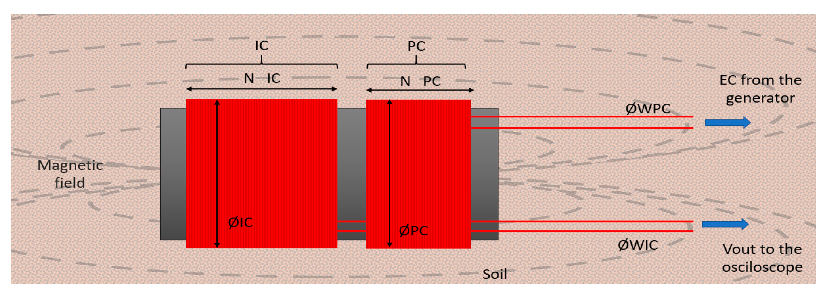
The principle stated before can be applied for environmental monitoring. In this paper, we propose several prototypes based on mutual inductance, which has been proven to be useful before [38,41]. The main novelty, according to the previous work [40], is the change in the monitored environment. In [41], the inductive coils were used to monitor the changes in the dielectric constant of a water body to estimate its conductivity or salt content. In this paper, the changes in the dielectric constant are related to the presence of water in the soil. In addition, as far as we know, there is no other work that analyzes the use of coils in different soils and including tests with the sensors buried for up to one month. Mutual inductance is a phenomenon with a principle stating that when a coil is powered with an electrical current (EC), a magnetic field appears. The characteristics of the said field depend on various parameters; among them, we find the diameter of the wire (ØW), the number of spires (N), the signal used to power the coil (both the frequency and the voltage influencing it), as well as the diameter of the powered coil (ØPC). As seen in Equation (1) and Ampere’s Law, the number of spires (N), the intensity of the current (I), and the permeability of the core of the solenoid (μ₀) determine the magnetic flux (B) of the solenoid. Moreover, there is an equation for an infinite solenoid in free space which is:

$$B={\mathsf{\mu }}_{0}N\mathrm{I}$$

(2)

Our prototypes were introduced in the soil, which contains water, with a relative permeability (μ_r). Since our prototype is finite, its length (l) should be considered in the formula as:

$$B=\frac{{\mathsf{\mu }}_0{\mathsf{\mu }}_{r}N\mathrm{I}}{l}$$

(3)

An increase in permeability is to be expected when adding water. It is to be noted that for “permeability”, we understand the resistance a medium presents to creating a magnetic field. Therefore, when it increases, the magnetic field increases, as well. Furthermore, the said increase in the magnetic field, which is most prominent in the ferromagnetic core (in the center of the solenoid coil), increases the flow of electrons, thus affecting the electrical conductivity of the medium. For our experiment, this core in the center of the solenoid coil was filled with soil with a varying amount of water.

When placing another coil in the vicinity of the PC, the magnetic field previously mentioned causes said coil to be induced. This phenomenon is better known as mutual inductance. A magnetic flux is created when the lines about the magnetic field formed by the PC go through the IC. All modifications to the medium containing the coils and, therefore, to the magnetic flux, will affect it. Changes in the water quantity (soil moisture) affected the output voltage also known as Vout. The formula of the mutual inductance is as follows:

$$M=k\sqrt{L1 L2}$$

(4)

Equation (4) shows the description of the mutual inductance of two solenoids (M). The parameters in that formula are k for the coupling coefficient and L1 and L2 for the inductances of the coils. The later ones are dependent on the number of turns (N), the length of the used solenoid (l), the core of each coil (μ₀μ_r), and the cross-section area in m² (A). The formula to calculate L1 and L2 with the aforementioned parameters is:

$$L1=\frac{{\mathsf{\mu }}_0{\mathsf{\mu }}_{r}NA}{l}$$

(5)

As stated before, the medium of the core determines the mutual inductance. For this experiment, the medium was soil. When the permeability experiences a change, the coupling effect (k) changes, as well. For the sake of the equation, it is important to note that the values for k range from 0, when no inductive coupling is present, to 1 (its maximum when there is a perfect coupling). A coupling effect of 1 implies that all the flux lines of the PC cut all the turns of the IC. For it to happen, the permeability should be high, and the coils should have a perfect geometry. One of the factors studied in our experiment is permeability, the characteristics of the core. Furthermore, the high number of prototypes tested is explained by the need to tests different geometries. Their position will be the same; nevertheless, the distance between the different coils and their length is one of the factors that change between prototypes.

Poljak et al. [42] performed a series of experiments in which they proved that the induced voltage depends on some characteristics of the coil (N, ØW, and the diameter of the induced coil, ØIC). Furthermore, they stated that Vout depends on μ_r and B. This principle, used for coils with a ferromagnetic core, is the power transformers’ principle.

The Biot–Savart Law [43]:

$$d\overrightarrow{B}=\frac{\mu }{4\pi }\frac{ \mathrm{i}\left(\mathrm{t}\right) \stackrel{\rightharpoonup }{dl}\stackrel{\rightharpoonup }{R}}{R^3}$$

(6)

The formula which determines the magnetic flux density is presented in Equation (6). The parameters on which it depends are the space of the source (R), a current which varies with time denoted by (t), the unit vector ($\stackrel{\rightharpoonup }{R}$), and the permeability (μ).

With Faraday’s Law, the induced electric field can be obtained:

$${{\displaystyle \oint }}_C^{}\overrightarrow{E}·d\overrightarrow{l}=\frac{-d}{dt}{{\displaystyle \int }}_S^{}\overrightarrow{B}·dS$$

(7)

In the above equation, a time-varying magnetic field (dφ) is determined by an inducted electric field around a closed path. The induced electric field, using Stoke’s theorem [44], can be defined in a non-varying surface (dS) by the number of turns (N), as in:

$${{\displaystyle \oint }}_C^{}\overrightarrow{E}·d\overrightarrow{l}=-N\frac{-d\phi }{dt}$$

(8)

Figure 1 presents all the considered variables in the experiments we conducted. Seeing the position of PC concerning the IC, it is to be expected that when there would be an increase in the generated magnetic field, it would reflect an increase or decrease in the Vout. Moreover, to further limit the variables, the signal used to power the PC had a fixed intensity and voltage in each set of tests, modifying the frequency.

The utility of this kind of sensor has been proved for water conductivity monitoring [41] and for monitoring the presence of fertilizers in water [38]. Several prototypes were tested in these experiments since it has already been proven that changing some variables (ØPC, ØIC, ØW, and N) is key in finding the best configuration. In this paper, we are trying to determine soil moisture based on its conductivity. Soil moisture is indicated as the water percentage in volume, as seen in Equation (9). Changes in soil moisture affect the dielectric constant, changing the permeability and producing a difference in the Vout. Soil moisture is indicated as the water percentage in volume as:

$$Soil moisture \left(\%vol\right)=\frac{Volume water \left(L\right)}{Volume soil \left(L\right)}$$

(9)

3.2. Prototypes

For the tests conducted, several prototypes were compared. They shared the same basic design with the coils winded on a PVC tube (3 mm of thickness). It is important to ensure that the core of the coils is full of soil since the magnetic flux is strongest there. Two sets of tests were be conducted; therefore, two types of prototypes were used.

3.2.1. Prototypes for the Initial Tests

In the first set of experiments, 15 prototypes were selected. They were named P1 through P15. They had varying ØW, ØPC, ØIC, Number of Spires (NS), presence or absence of casing, number of layers, and windings ratio. The windings ratio is the coefficient between the NS of the PC and IC. The characteristics of the prototypes can be seen in

Table 1. Features of the different prototypes for the initial tests.

Prototype	ØW (mm)	Layers	Casing	ØPC and ØIC (mm)	Ø Casing (mm)	NS PC	NS IC	Windings Ratio
P1	0.4	1	Yes	20	28	40	40	1:1
P2	0.4	1	Yes	20	28	40	100	1:2.5
P3	0.4	1	Yes	20	28	100	40	1:0.4
P4	0.4	8	Yes	25	43	40	80	1:2
P5	0.4	8	Yes	25	43	80	40	1:0.5
P6	0.4	4	Yes	25	43	40	80	1:2
P7	0.4	4	Yes	25	43	80	40	1:0.5
P8	0.4	1	No	25	-	5	10	1:2
P9	0.4	1	No	25	-	10	5	1:0.5
P10	0.4	1	No	25	-	10	20	1:2
P11	0.4	1	No	25	-	20	10	1:0.5
P12	0.4	1	No	25	-	20	40	1:2
P13	0.4	1	No	25	-	40	20	1:0.5
P14	0.6	1	No	25	-	20	40	1:2
P15	0.6	1	No	25	-	40	20	1:0.5

. The best windings ratio for this type of sensor has been proven in previous papers to be 1:0.5 and 1:2 [41]; hence, most prototypes have this value. The other three prototypes (P1 to P3) had winding ratios similar to the aforementioned ones. To keep the experiment simple, the diameter of the coil (ØC) and the ØW for both coils were the same. The ØC was 25 mm for all the prototypes. Meanwhile, the ØW was 0.4 mm for P1 to P13, since it was the one that presented the best results in [41], and 0.6 mm for P14 and P15. Moreover, the use of casing (1 mm of thickness) for the coils was tested to evaluate if the extra PVC tube isolation would affect the measures. Furthermore, four of the prototypes had their spires in multiple layers. Some prototypes, with and without casing, can be seen in Figure 2.

3.2.2. Enhancement of the Pre-Selected Prototype

The prototype with better results was selected for the creation of 4 new prototypes. These sensors (NP1 to NP4) exploited the best windings ratio. Moreover, they introduced a new winding ratio with several spires similar to the best prototype out of the 15 first ones. All of the new sensors had their spires in one layer; they were similar to P8. Furthermore, to minimize the error when connecting the sensors, they had all the elements necessary for the circuit already connected to the sensor, turning them into a fully functional sensor. Their characteristics can be seen in

Table 2. Features of the prototypes NP1 to NP4.

Prototype	ØW (mm)	Layers	Casing	ØPC and ØIC (mm)	NS PC	NS IC	Windings Ratio
NP1	0.4	1	No	25	5	10	1:2
NP2	0.4	1	No	50	5	10	1:2
NP3	0.4	1	No	25	15	10	1:0.67
NP4	0.4	1	No	50	15	10	1:0.67

. Note that NP 1 is equal to P8.

3.3. Circuit Characteristics and Measurement Protocol

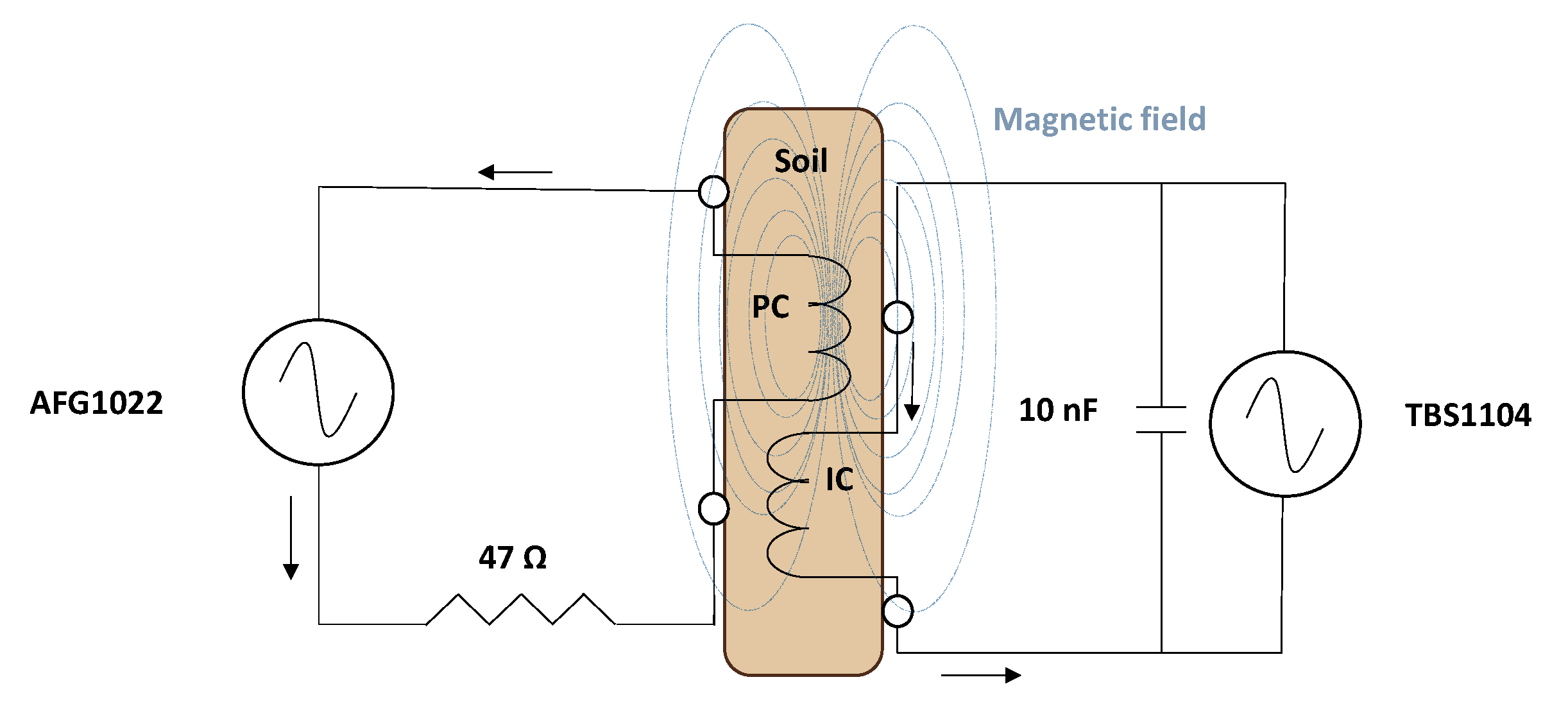
A power generator was the source of the EC for the PC (a sinus-wave); the AFG1022 from Tektronix [45] was selected. The range of frequencies it can generate and it is user-friendly handling fostered the selection of this generator. For the initial tests, a voltage of 10 Vpp was used. This was chosen to amplify the variances between the different Vout values. The objective of these tests was to determine the best configuration out of the very different P1 to P15 prototypes. Nevertheless, for enhancement tests, the voltage chosen was 3.3 Vpp. This is the standard voltage at which Arduino works. Therefore, it is best to adjust the equations derived from sensors NP1 to NP4.

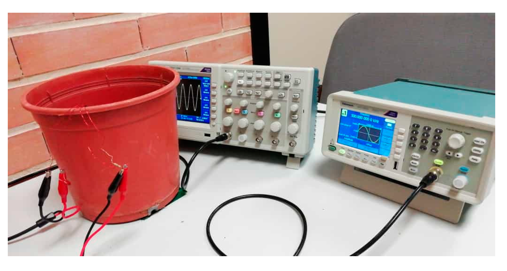
For both sets of tests, the selected oscilloscope to register the Vout was the TBS1104 from Tektronix [46]. Furthermore, a resistance of 47 Ω on the positive wire of the PC was added to protect the oscilloscope and reduce peaks, as well as a capacitor of 10 nF, which was connected to both wires on the IC. This assembly, see Figure 3, is based on [41].

It is to be noted that each datum for this experiment in the results section corresponds to the mean of five repetitions. The Vout reading was taken in quintuplicate, thus making the results more rigorous. To simplify the analyses, standard deviation data will only be presented when calibration tests were performed.

Next, the measurement protocols for each set of tests are described. For the initial tests, two experiments were conducted. In the first test, we used all the prototypes described in Table 1, focusing on a narrow range of useful frequencies which present big differences between the Vout of different moisture values. The peak frequency (where the highest Vout is measured) and the ones close to it. We compromise to a low number of samples to test the 15 prototypes. Using five samples allowed us to test all 15 of them with a degree of certainty. After finishing the first experiment corresponding to the initial tests, the best prototypes were selected. The criteria used were the requirements stated in Section 2. The selected prototypes were used to perform the second experiment for the initial tests.

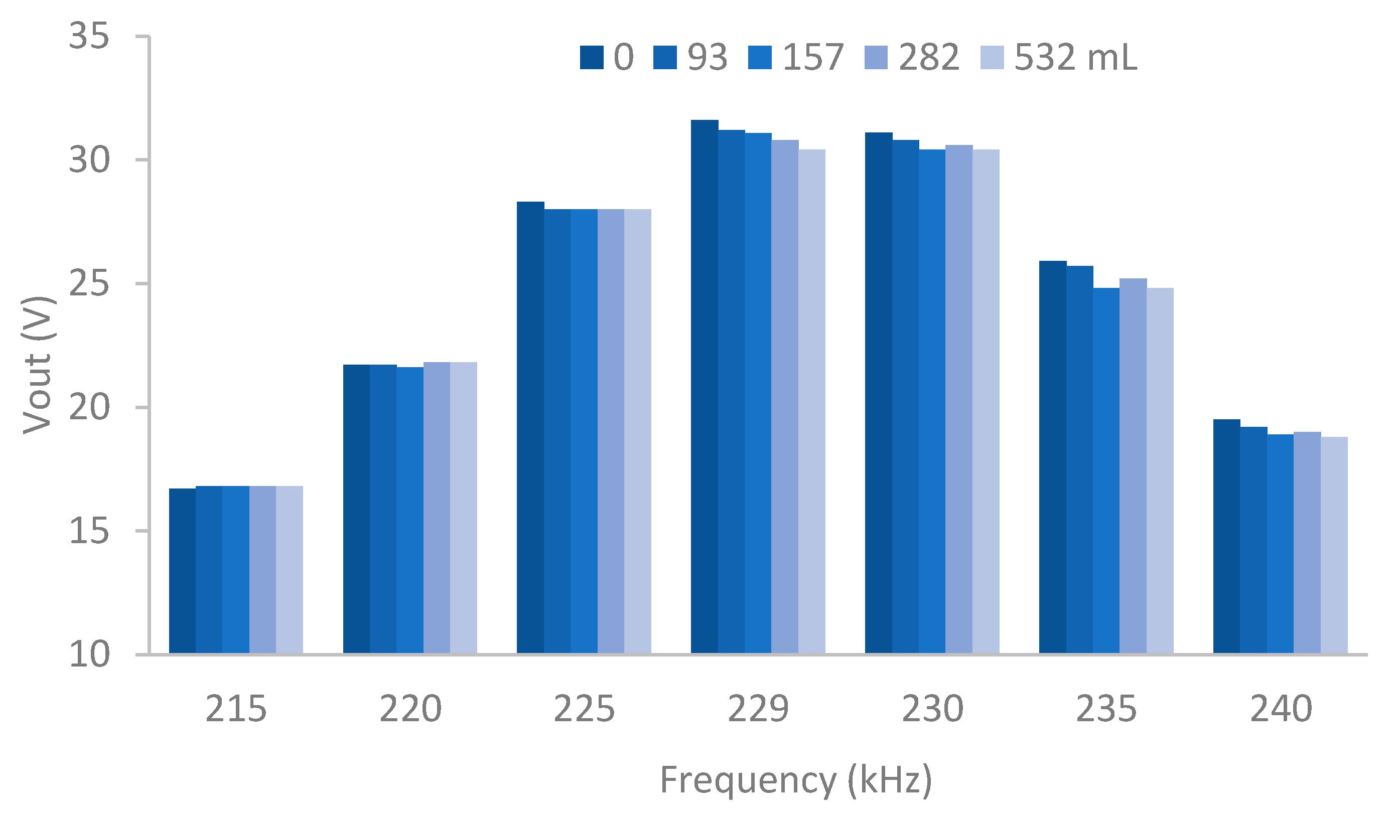
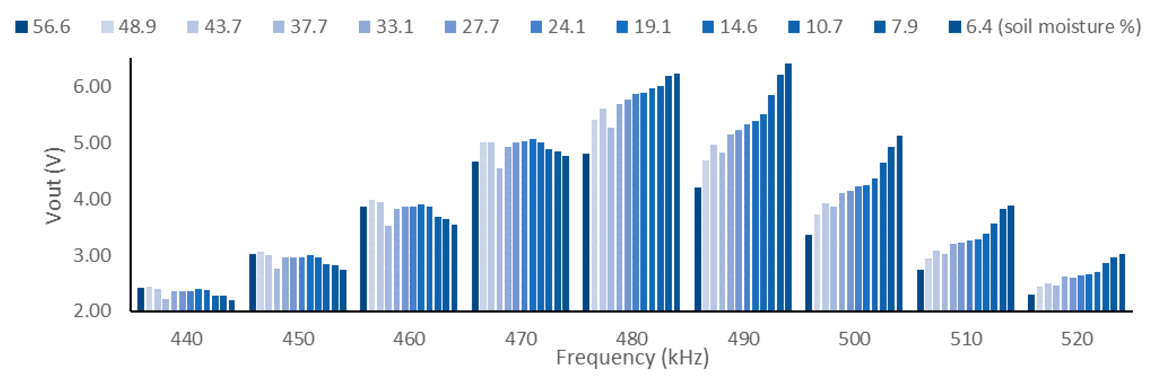
Once the best prototypes were defined, further tests were performed. These tests were conducted to test the performance of our sensors when kept on the soil all the time. The prototypes described in Table 2 were used for this experiment. The frequencies used for this set of tests were those close to the peak. The peak frequencies are determined in the different samples when the soil has the maximum moisture tested. In these conditions, we search the peak frequency in the range of 0 to 1 MHz. Once the peak frequency is found, we measure at the frequencies of ±10, 20, 30, and 40 kHz of peak frequency. This range was chosen because it represents the frequencies where the sensor shows a higher sensitivity to changes in the environment and displays a higher output voltage. These experiences allowed us to check the effectiveness of the sensors for a different soil type.

While for the first set of tests, the sensors are inserted and extracted from each pot every time the soil moisture is measured, for the second set of tests, the sensors were left inside the pots throughout the entire experiment. This modification in the measurement methodology was conducted to evaluate if the continuous introduction of the sensor might cause an alteration in the measurement by including interferences. Those interferences can be caused by the lack of homogeneity of the soil (different compaction, the apparition of preferential water channels, etc.) provoked by its continuous manipulation. Measurements were taken daily for as long as the tests were conducted. The objective of these experiments was to prove the usefulness of keeping the sensors buried, to minimize the errors from extracting and inserting them. Furthermore, since the soil was different, these experiments wanted to test the efficiency of the prototypes for a crop during harvest.

3.4. Soil Samples

In this subsection, we describe the soil samples used in the first and second set of tests and their variability in soil moisture along the experiments. The different soils were obtained during summer in the La Safor region (Valencia, Spain). The soils are a representation of typical farmer soils of this region. Considering that collected cannot be classified as unaltered samples since they are sifted and water was added to the soil, the specific ambient conditions in which the samples are collected are not relevant. The soil screening was carried out to avoid creating preferential water channels that could affect the measurements and homogenize the samples.

3.4.1. First Set of Tests: Selection of the Best Prototype/s

For the soil samples used in the initial tests, plastic pots shaped like a conical trunk were employed. Their dimensions were 18.9 cm in height, 16 cm of minor radius, and 20.5 cm of major radius. The pots were filled with soil and a variable volume of water for the experiments. Depending on the experiment, we used up to five types of soil.

The used sample for the first experiment was a commercial soil composed of peat and manure, used mostly for gardening, with high sand content. Therefore, the soil moisture levels tested were close to the FC and WP presented by sandy soils—20% and 7%, respectively. Furthermore, the soil used for this experiment came from the same lot to prevent other factors from affecting the results. We started with dry soil, with 0% soil moisture, and water was added to create the samples, homogenizing them to guarantee soil uniformity; each sample contained 3 kg of soil. The five samples of soil presented volumetric water contents from 0% to 27% (M1 to M5); see

Table 3. Characteristics of the pots, first test.

	M1	M2	M3	M4	M5
Volumetric water content (%)	0.00	3.59	6.21	12.57	26.91
Water (mL)	0	93	157	282	532

. A picture of the samples used in this experiment can be observed in Figure 4. In addition, Figure 5 presents the assembly for the tests where we can see the scheme of the experiment, with the oscilloscope, the pot, the generator, and the wires.

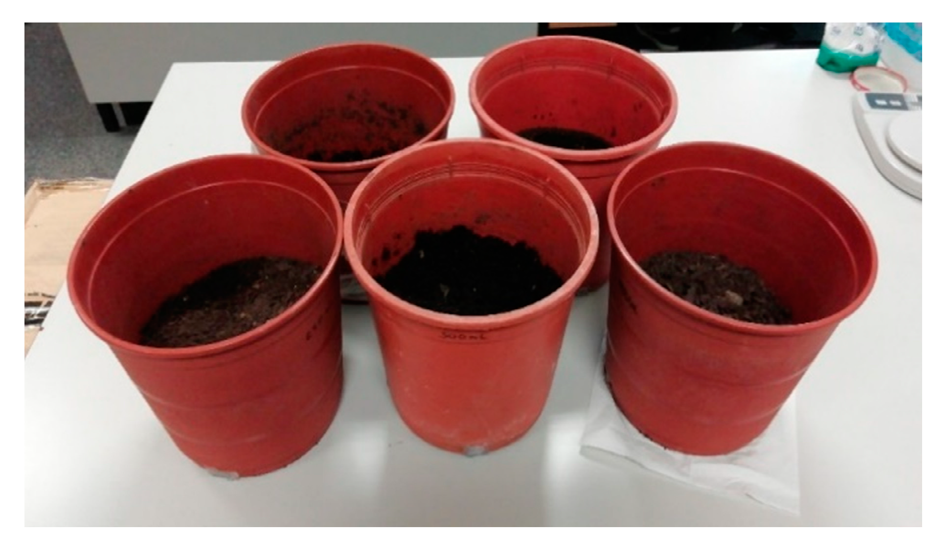
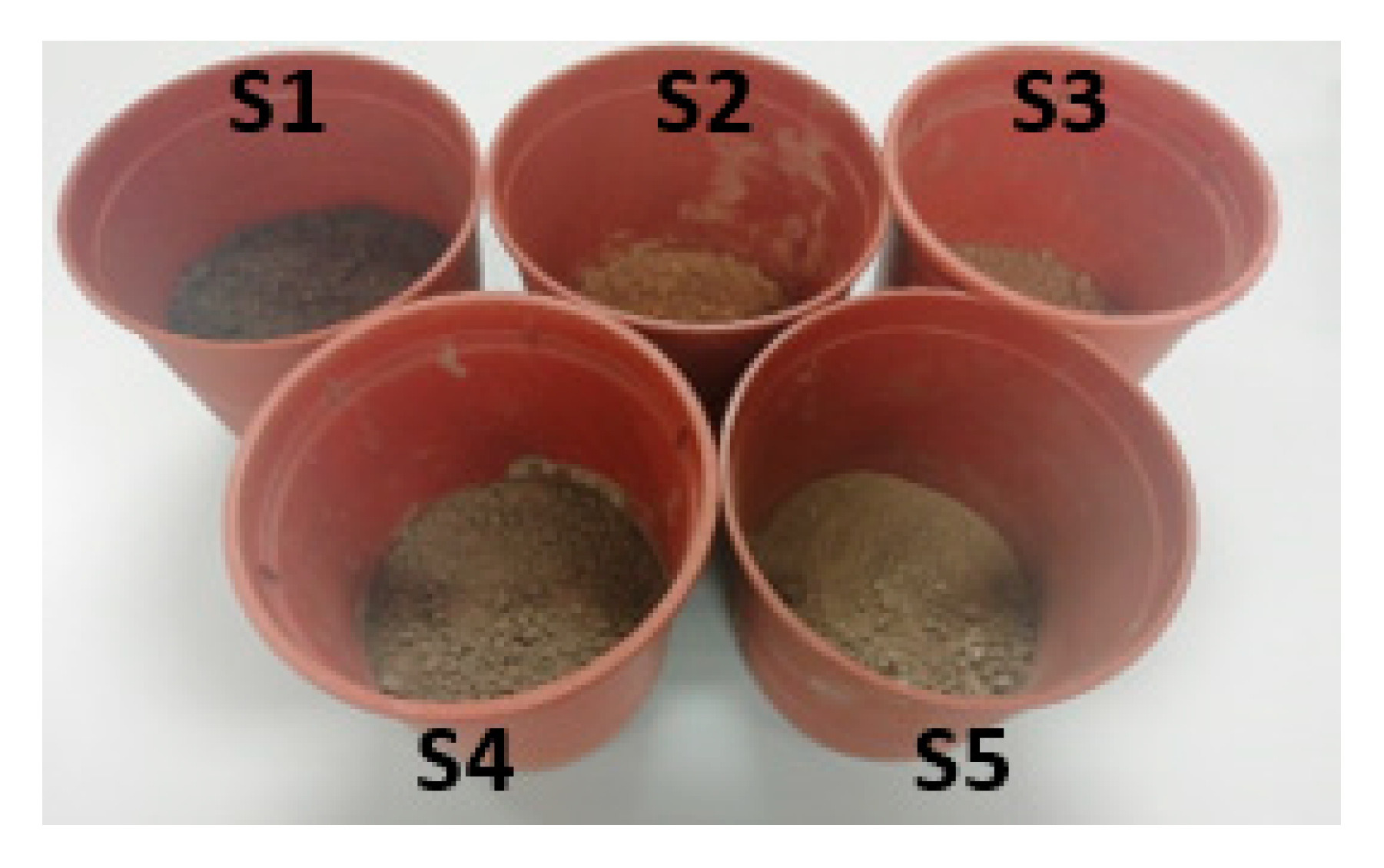
Samples from 5 different types of soil (S1 to S5) were used in the second part of the first set of experiments. The first type of soil, S1, was the one used for the previous test. S2 was obtained from a former citrus crop. S3 was gathered from calcareous soil in a mountain. Finally, two crops near the coastline provided the soil for S4 and S5. All the samples were taken from the region of Valencia, Spain. In order to prepare the samples, the following protocol was used. First, with a shovel and a recipient to put the soil in, the samples were collected. It was important to avoid rocks and plants to ease the process after the collection. Next, the clods and clumps of soil were crushed with the help of a tray and a rolling pin. In this step, all the rocks, plants, and possible invertebrates present on the soil were manually removed. Afterwards, using a 2 mm aperture sieve, the soil was filtered until we had a kilo and a half of the sample. The pots used for this test have the same characteristics as the ones used for the first one. The pots with the different soil types can be seen in Figure 6. To estimate the volume of soil in each pot, the major radius at the top of the soil and its height were measured. Moreover, the minor radius was measured.

The soil moisturizing process for this assay was more precise than for the previous experiment. Since the objective of this test was to find the best prototype/s, it needed to be more accurate. The first step was to seal the bottom of the pot with filter paper, making water able to infiltrate the pot, so soil cannot fall out. The result was weighed, and afterwards, 500 g of soil was added. The pots, alongside the filter paper and soil, were submerged in water up to one cm under the soil level. When the top of the soil started looking wet, 500 more grams were added, and the pot was further submerged. The process was repeated a third time. This was carried out to fill with water all the gaps between soil particles and saturate it. The pots were left for 24 h at 25 °C to rid the excess water.

With weight measures, the mass of water can be obtained, and water volume is easily related to its weight. We used 1.5 kg of each soil. Nevertheless, the parameter needed to calculate the real soil weight is the original soil moisture. To calculate the weight of the dry soil, five samples of around 20–25 mg were prepared, one for each type of soil. They were weighed and then dried at 105 °C. This was performed to evaporate all water present in the samples. Then, the dry sample was weighed to calculate the % of dry soil using:

$$\mathrm{Dry} \mathrm{soil} \%=\frac{\mathrm{Weight} \mathrm{of} \mathrm{dry} \mathrm{soil} \left(\mathrm{g}\right)}{\mathrm{Initial} \mathrm{weight} \mathrm{of} \mathrm{soil} \left(\mathrm{g}\right)}\ast 100$$

(10)

3.4.2. Second Set of Tests: Enhancement of the Pre-Selected Prototypes

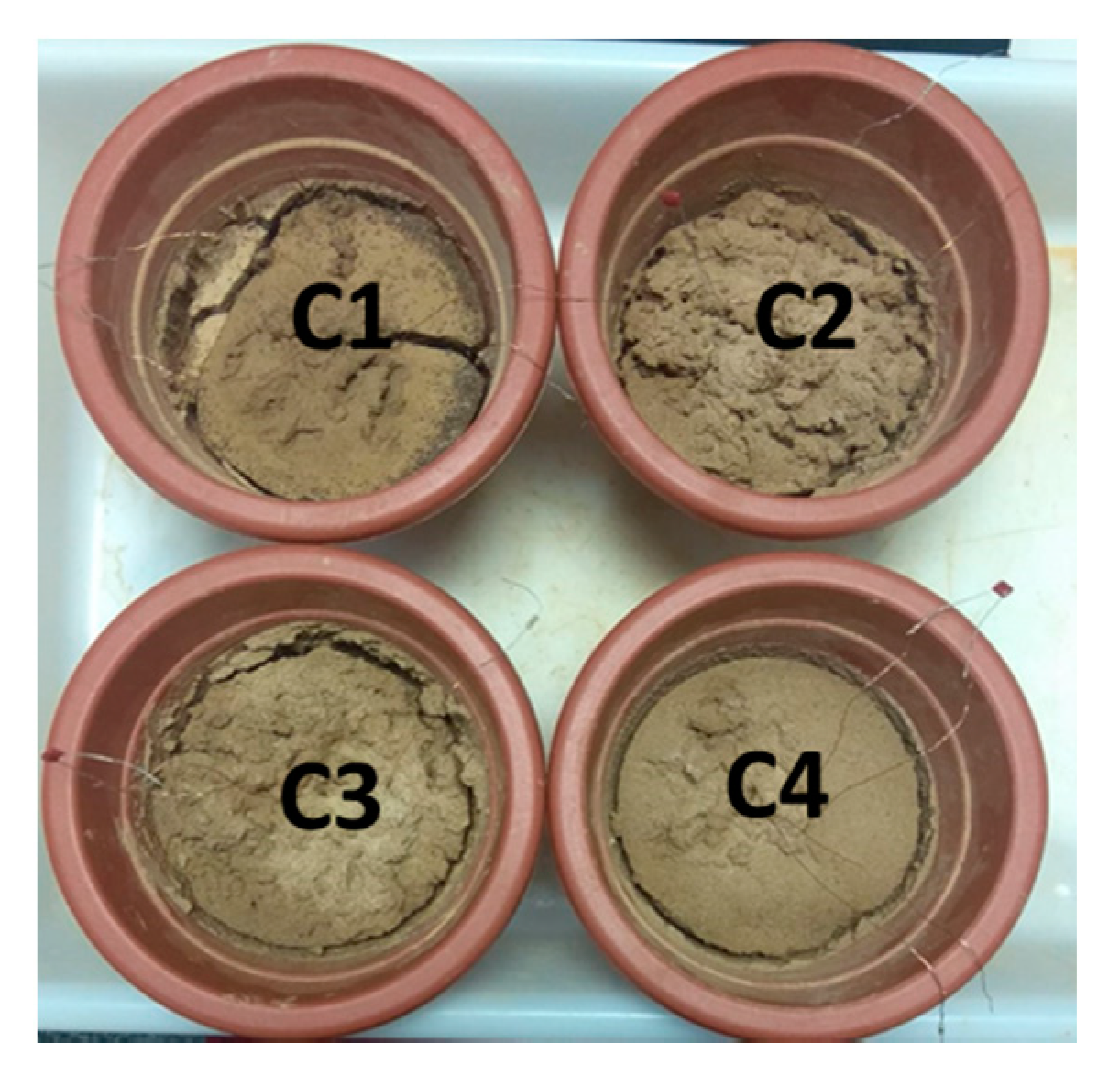
A sole type of soil was used. Nevertheless, it was different from the previous types, and four repetitions were used (C1 to C4). The soil was a sandy type extracted from an orchard field.

The pots used for these tests were smaller, with a maximum radius of 6.65 cm. A total of 1 kg of each soil was inserted in each pot. A sample was taken from the original soil and dried in order to obtain the moisture percentage to calculate the dry soil. In Figure 7, the pots of soils C1, C2, C3, and C4 are depicted. Regarding the procedure of soil moisturizing, we followed the aforementioned moisturizing process, which consists of adding small quantities of soil and letting water saturate all the gaps of soil.

3.4.3. Soil Samples Characterization

The soil characterization for both samples for the initial tests (S1–5) as well as for the enhancement of the pre-selected prototypes (C1–4) can be seen in this subsection. The soil weight characteristics, the original % of dry soil, and the derived weight values for the soil moisture estimation by weight are presented in

Table 4. Soil characteristics.

	S1	S2	S3	S4	S5	C1–4
% Dry soil	35	84	80	92	80	97.6
Total weight of the dry soil (g)	525	1260	1200	1380	1200	976
Weight of the pot and filter paper (g)	149	149	125	125	149	87
Weight of dry soil + pot + filter paper (g)	674	1409	1325	1505	1349	1063
Sand (%)	100	60	70	95	90	80
Silt (%)	0	30	23	3	6	15
Clay (%)	0	10	7	2	4	5

. The measures of the pots, as well as their volume, are presented in

Table 5. Pot characteristics.

	S1	S2	S3	S4	S5	C1–4
Minor radius (cm)	8	8	8	8	8	4.55
Major radius (cm)	8.5	8.75	9	8.75	9	6.65
Height (cm)	10.5	5	6	4	4.5	7.04
Volume (cm3)	2246	1103	1363	882	1023	697.7

. Furthermore, the results for the soil moisture measures are presented in

Table 6. Summary of the soil moisture variations.

	S1	S2	S3	S4	S5	C1	C2	C3	C4
Initial water percentage (%)	75.21	43.45	51.19	36.36	32.66	57.2	56.6	63.1	59.3
Final water percentage (%)	51.61	14.60	22.74	0.00	16.43	7.0	6.4	8.5	7.5
Soil moisture variation (%)	23.60	28.84	28.46	36.36	16.23	50.2	50.2	54.6	51.8

; this information will help understand the results. It presents the soil volume, the initial and final water volume, and their variation.

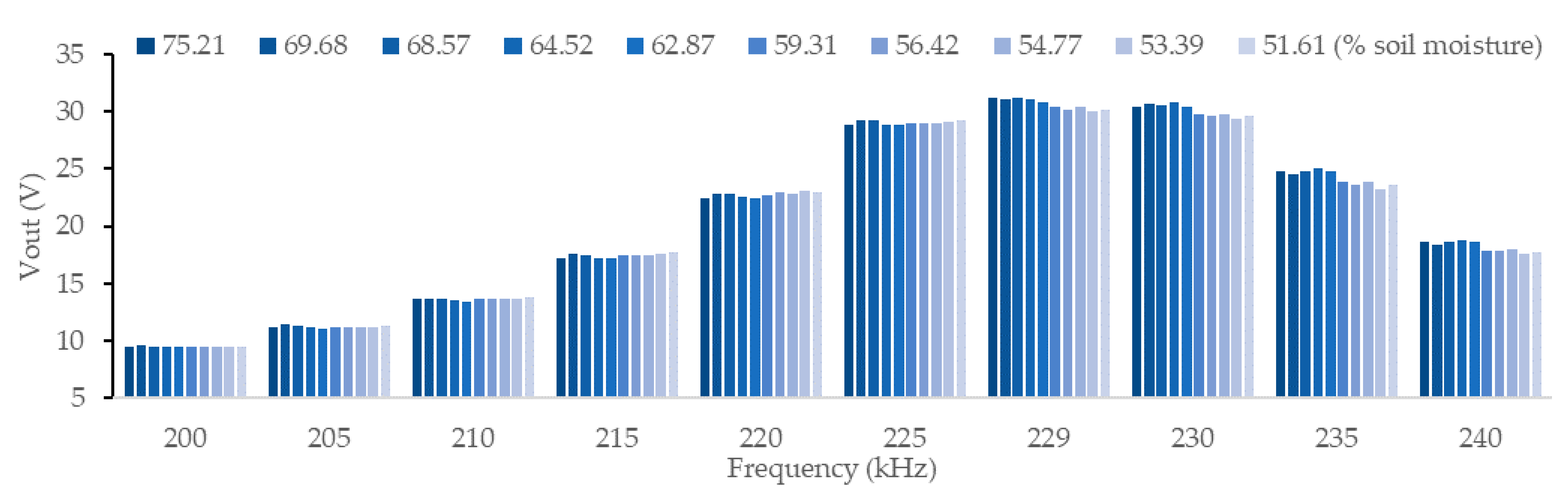
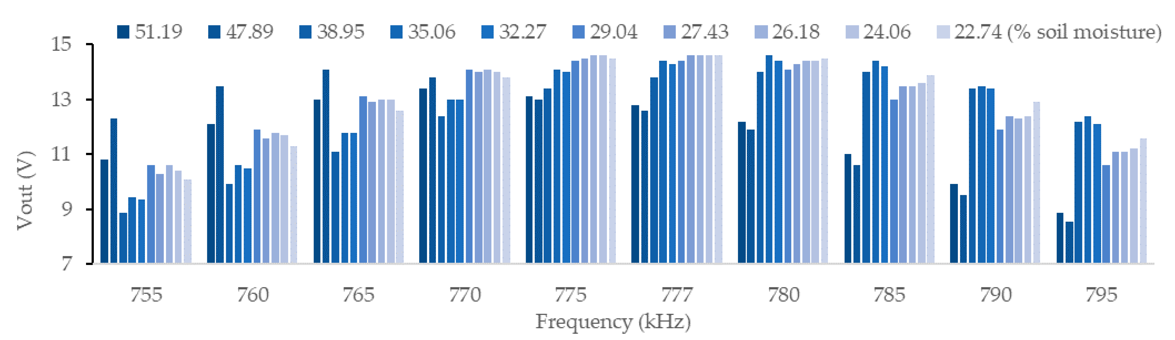
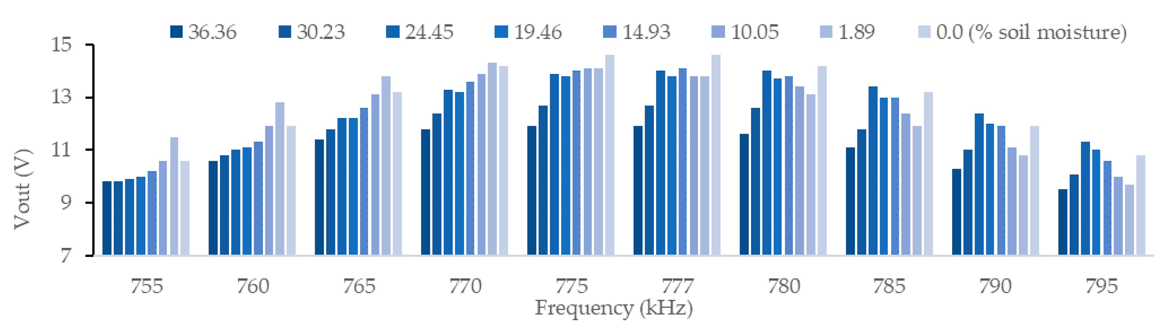
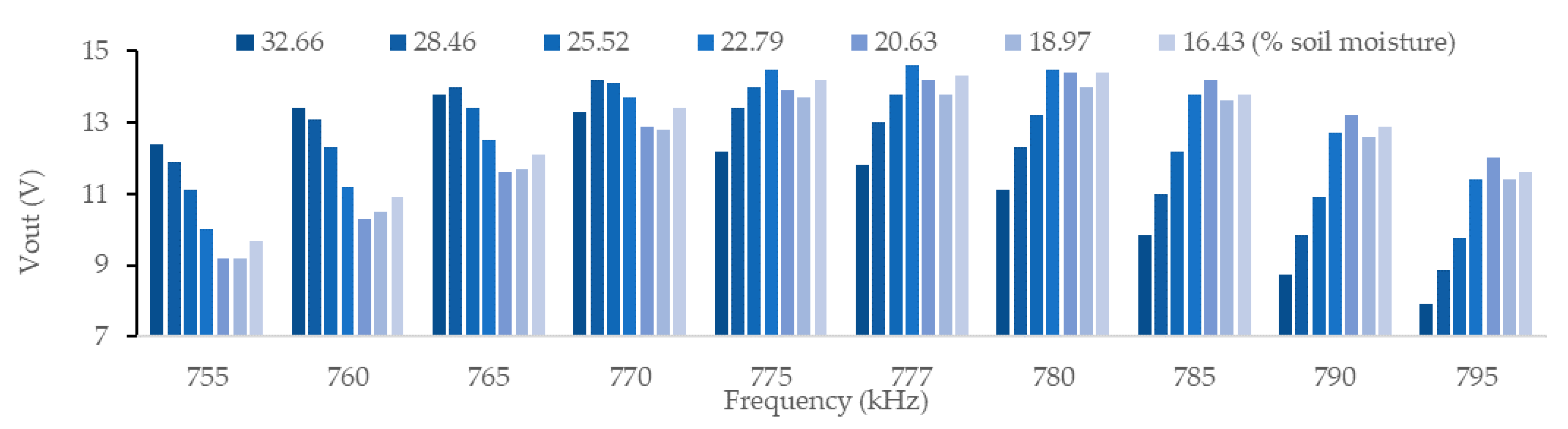
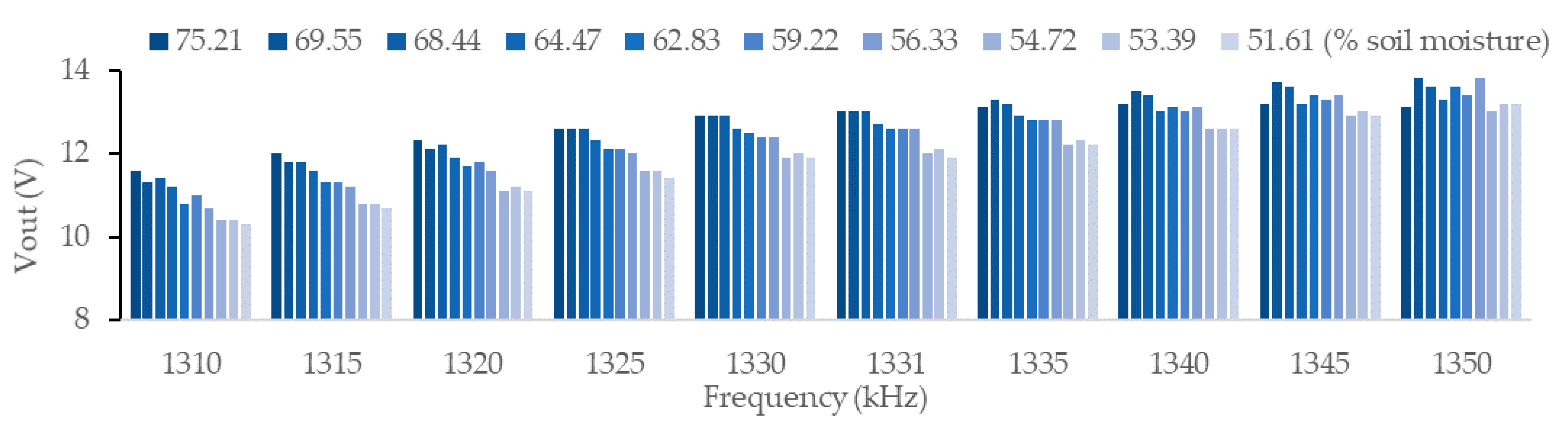
S1 to S3 could be measured for the duration of the experiment, a total of 10 days. Meanwhile, S4 and S5 could only be tested for eight and seven days each. This is because S4 was completely dried on the seventh day, and the last three measures for S5 gave the same reading, 16.23%. Due to the high organic matter content, S1 retained more water than the other samples, which preclude reaching the WP during the tests. The lowest soil moisture percentage measured on this soil was 51.61%. On the contrary, both S2 and S4 were tested from FC to WP. S2, composed of 60% sand and 30% of silt, have its WP of around 15% soil moisture. In S4, being sandy soil, the FC should be at around 24% and the WP at around 7%. Considering that both these limits have been surpassed, we can conclude that the analysis encompassed both points. S3 and S5 are in a similar condition to S1. The final soil moisture is higher than the WP, although in the case of S5, we could assume it is the WP due to the water being strongly retained in the soil.

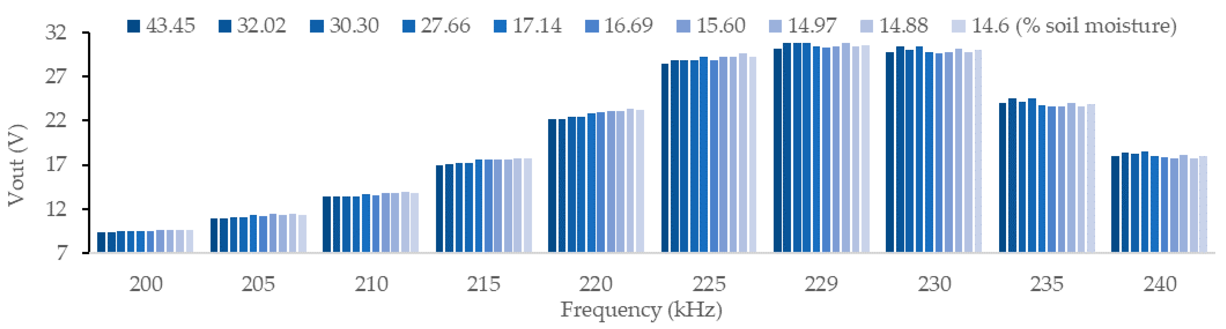
The behavior of C1–4 is similar since they come from the same lot. All of them started at around 55–65% soil moisture and ended close to 6–9%. The target range was studied because sandy soils have their FC at around 24% and their WP at around 7% [5].

4. Results and Discussion

In this section, the results of the aforementioned tests are presented. Initially, we show the data from prototypes P1 to P15. Next, the results from the best prototypes on five different soil types are shown. Then, the calibration of the best prototypes is presented. Finally, the results from the enhancement tests are explained.

4.1. Test at Peak Frequencies for P1 to P15

This subsection shows the results of the tests performed with P1 to P15. Only the frequencies close to the peak frequency were analyzed to test these prototypes. We defined the peak frequency with the sample of 0% of moisture; it has been proven that peak frequency changes with the environment [38]. First, we discuss the prototypes which were not found suitable for further testing. Next, the prototypes which were used for further tests are explained.

The first prototype analyzed is P1. Its peak frequency is not consistent throughout the measurements shifting between 270 and 267 kHz. This prototype is not suitable for moisture monitoring because M1, M2, and M4 have similar Vout values, and they are different from M3 and M5. When analyzing P2, the first thing to be noticed is that almost no change was presented between the different moisture levels for some frequencies—going as far as the Vout being the same from M1 to M4 for 160 kHz. The maximum Vout detected is 32.8 V at the peak frequency (149 kHz) for M1 and M5. The fact that the Vout for the two extremes of the tested moisture levels were the same is another indicator of the unsuitability of this sensor. There is nothing remarkable for P3. Many of the tested frequencies present the same value for two different moisture levels, for example, 10.6 V for M1, M3, and M4 at 2555 kHz. The peak for this prototype is 25.7 V at the peak frequency (267 kHz) for M2. None of the tested frequencies presents a trend, thus rendering the prototype not useful for this study.

P4 could be a promising prototype as (i) the Vout for different samples is high, 47 to 48.8 V; (ii) the difference between M1 and M5 is high, 1.9 V; and (iv) its working frequency is low, 115 kHz. Nevertheless, the Vout in the promising frequency (115 kHz) for two different moisture levels (M2 and M3) was the same, 47.6 V. Moreover, the high dispersion between the different measures makes P4 unreliable.

Following, the data obtained from P6 and P7 are analyzed. P6 exhibits the highest Vout (50.8 V) at its peak frequency (112 kHz). Nonetheless, no relationship between soil moisture and Vout is found at any of the measured points. For P7, a maximum Vout of 32.2 V is recorded for M1 and M3 at the peak frequency (210 kHz). As in P6, it does not appear to exhibit a direct relationship between soil moisture and Vout at any of the frequencies. P6 and P7 cannot be recommended to be used as soil moisture sensors.

P10 and P11 are assessed in this paragraph. In M3, P10 exhibits a maximum frequency of 366 kHz and a maximum Vout of 30.1 V. This prototype presents no point at which the prototype can be used to distinguish the moisture values since the Vout at M3 and M4 are higher than the other moisture levels at all tested frequencies. The maximum Vout for P11 is presented at M3, with a value of 25.5 V at a frequency of 585 kHz. According to gathered Vout values, P11 can be considered a good choice for measuring humidity at 595 kHz. Using a sigmoid function to the soil moisture values, the Vout data at this frequency can be adjusted correctly. Nevertheless, considering that the sensor response is only accurate in 0–6.21%, this mathematical model is not useful.

The data for P12 and P13 are presented below. P12 exhibits a maximum Vout of 34.5 V for M4 with a maximum frequency of 209 kHz. Similarly, P13 exhibits a maximum Vout of 30.4 V for M4 with a frequency of 340 kHz. In the case of P12, it exhibits a decrease with increasing water content and then an increase. The Vout for M1 is higher at various frequencies than the Vout for M5, making this sensor unsuitable for soil moisture monitoring. On the contrary, in the case of P13, the Vout has no trend at all. P13 is not suitable for soil moisture monitoring.

Following, the data from P14 and P15 are analyzed. The highest Vout presented by this sensor is 24.8 V for M2, with a frequency of 317 kHz. For each tested frequency, the behavior of the Vout with increasing water content is different. Because of the disparity of results and their inconsistency, this sensor cannot be used for soil moisture monitoring. For M2 and M5, P15 has a peak frequency of 530 kHz; for M3 and M4, a peak frequency of 353 kHz; and for M1, it is 528 kHz. Although the Vout is high and differences between different moisture levels are appropriate, they do not follow a trend (ascending or descending). Therefore, this prototype is not suitable for the purpose of this experiment.

Next, the data for the prototypes that will be used for further tests are presented. First, Figure 8 represents the data of P5. The peak frequency, found at 229 kHz (31.6 V), presents a decreasing trend for the Vout, which could be of interest. Thus, P5 meets the requirements: high Vout (around 30–31 V), high Vout difference between M1 and M5 (1.2 V), different Vout for each moisture level, and low working frequency of 229 kHz.

Concerning P8, it presents reasonable voltage differences (over 0.5 V in most cases) as well as an overall high Vout, as can be seen in Figure 9. It presents three peak frequencies on the tested spectrum, although they are all low enough to accomplish (iv). Furthermore, a descending trend can be observed for 780 kHz. The only problem for this prototype is that two data from 780 kHz present the same Vout, not accomplishing (iii). Nevertheless, P8 is interesting and will be included in further tests.

Figure 10 represents the results of P9. The first thing to be noticed is the trend presented at 1315 and 1320 kHz. The Vout for this prototype is high, and the differences are noticeable (higher than 0.1 V). The difference between M4 and M5 is higher than the others, which is not uncanny taking into account M5 is almost twice as moist as M4. There is a minor issue with P5, its working frequency, which is too high, not accomplishing (iv). Nonetheless, it is a promising prototype that should be further studied.

To summarize our results,

Table 7. Requisites that accomplish each prototype (“x” indicates prototype accomplish the requisite and “–” does not accomplish).

Requisites	Prototypes
	P1	P2	P3	P4	P5	P6	P7	P8	P9	P10	P11	P12	P13	P14	P15
(i)	x	x	x	x	x	x	x	x	x	x	x	x	x	x	x
(ii)	–	–	–	x	x	–	–	x	x	–	–	–	x	x	x
(iii)	–	-	–	–	x	–	–	–	x	–	–	–	–	–	–
(iv)	x	x	x	x	x	x	x	x	-	x	x	x	x	x	x

shows which requisites are accomplished or not by every prototype. P5 accomplishes all requisites, being ideal for the tests. P8 and P4 only fail to accomplish one requisite (repeated values). Despite this, the differences between the Vout for M1 and M5 for P4 are significantly lower than for P8. Furthermore, P4 presents a higher dispersion between the values to calculate the mean value used for this experiment. Moreover, we expect that the issue with P8 will not be reproduced in other soil types. Finally, although P9 does not accomplish (iv), it is the less problematic requisite. Those are the reasons why the chosen prototypes for further tests are P5, P8, and P9.

4.2. Secondary Tests

In this subsection, the calibration and verification of the selected prototype for different sorts of soil are shown.

4.2.1. Results for P5

For S1, P5 has a peak Vout of 31.2 V between the highest soil moisture located between 75.21% and 64.21%. The best frequency is 229 kHz, presenting a decreasing trend that could be further analyzed, as seen in Figure 11. The difference displayed in the voltage between the soil with a high amount of water and minimum soil moisture is about 1 V. Furthermore, a voltage change of 0.2 V is observed between the different moisture contents. The P5 for S1 is able to measure between 51.61% to 75.21% of moisture. Therefore, this prototype may be useful for S1 with elevated water content.

Figure 12 displays the data gathered from P5 on S2, which show an increasing trend of Vout with the increase in soil moisture up to the peak frequency and a decreasing trend afterwards. The peak is located at 229 kHz frequency. This frequency shows the highest value changes, about 0.6 V, between the maximum soil moisture levels (43.4% and 32.01%). The voltage changes between the different moisture contents are relatively low, being in most cases between 0.1 V to 0.4 V. Besides, the 225 kHz frequency seems to be more efficient to differentiate between low moisture between 14.96% and 16.68%. The P5 for S2 shows a correct behavior for high moisture at the 229 kHz frequency and low moisture at the 225 kHz frequency.

P5 on S3 has a peak frequency of 229 kHz. In this case, the frequency where the greatest differences are found in the 225 kHz frequency. The last frequency shows increasing values as the moisture content decreases. The highest voltage is recorded at the moisture content of 27.43% with 29.2 V and the minimum 28.4 V. The highest difference is 0.8 V. The measures do not seem to show a pattern. Therefore, this P5 is not useful for S3.

We tested the P5 on S4 and small changes can be observed between the different moisture ranges from 0.2 V to 0.3 V at the 225 kHz frequency. The largest difference is found between the 36.35% and 30.23% moisture with a change of 0.3 V. At all other moisture, the voltages are not stable, making it impossible to measure the moisture. Since it shows no pattern for this soil type, P5 is discarded for this S4.

Finally, for P5 on S5, the peak frequency is 229 kHz (similar peak on all soils) with a Vout of 30.9 V for soil moisture of 22.79%. The voltage difference between the different moistures is very heterogeneous, with the largest change of 0.9 V between 25.52% and 22.78%. On the contrary, between the other moisture levels, the difference is 0 V or 0.1 V. The data do not appear to display a trend. Furthermore, the voltage changes between the highest and lowest moisture are irrelevant. This means that P5 is not useful for S5.

The overview of P5 is that S1 and S2 are the soils for which the prototype is recommended to monitor the moisture. This is because they show larger voltage differences between the highest and lowest moisture in the 0.6 V to 1 V range. Furthermore, the differences between contiguous moisture values are in the range of 0.2 to 0.4 V.

4.2.2. Results for P8

For S1 and the prototype P8, the maximum voltage change between the maximum and minimum moisture content is 0.5 V. Moreover, no significant changes are observed between the different moisture levels, and no trend is observed in the data obtained. Therefore, this P8 is not recommendable for monitoring S1. In S2, P8 shows similar results.

Figure 13 displays the results of P8 for S3 where a trend of increasing Vout values is observed with soil moisture values after the 775 kHz frequency. The lowest voltage values, 13.1 and 13 V, are found in the higher soil moisture range (51.19% and 47.89%) and higher Vout values, 14.5 to 14.6 V, in higher moisture ranges (27.43% to 22.74%). At this frequency, we observe that the voltage difference between the different moisture levels is high and decreases as the soil moisture decreases. P8 might be used for S3.

Another sandy soil (S4) using P8 shows a clear increasing trend up to the peak frequency. The data gathered in this specific test are shown in Figure 14. The frequencies higher than 777 kHz do not seem to follow a trend. At the peak frequency, 770 kHz, the Vout changes between high soil moisture are very noticeable (approximately 0.5 V), decreasing as the soil moisture decreases. Furthermore, the voltage changes between the different moisture levels are in the range of 0.1 V to 0.9 V. The 770 kHz frequency, although not the peak frequency, shows an appropriate trend to be used for humidity measurement. In addition, the output voltages increase as the moisture content decreases, starting at 11.8 V for 36.35% and ending at 14.2 V for 0% moisture. Thus, P8 are suitable for S4.

Finally, results of P8 using S5 are analyzed. In this case, the best frequency for moisture monitoring is not at the peak frequency but at the frequencies close to it, exactly at 755 kHz. The latter frequency shows a voltage change of 2.72 V between the maximum and the minimum. Furthermore, the voltage changes between the different measured moisture levels vary in the range from 0 V to 1.1 V. The trend also shows a downward disposition. Figure 15 displays high differences between two contiguous measures in the presented soil. For this S5, P8 presents a good performance.

P8 can be used to monitor soils S3, S4, and S5. The interesting frequencies for use in mathematical models are as follows: for S3, 775 kHz; for S4, 770 kHz; and for S5, 755 kHz. Each type of soil has its own characteristics, depending on its composition. In this case, this prototype is ideally suited for measurements on S3–S5, but not for S1 and S2.

4.2.3. Results for P9

The case of P9 in S1 presents a decreasing trend of the Vout between the frequencies 1310 to 1331 tested, as seen in Figure 16. The frequency that shows a clear trend is 1315 kHz. This trend is decreasing as the moisture percentage is reduced, starting with 12 V for maximum moisture and ending with an output voltage of 10.3 V for minimum moisture. This frequency shows a voltage change in the range of 0.2 V to 0.5 V between the different moisture levels recorded. On the highest frequency (1350 kHz) for 56.33% soil moisture, the peak Vout is 13.8 V. This is probably due to an experimental failure rather than a poor performance of the sensor in this type of soil. Moreover, the frequency 1325 kHz also shows a decreasing trend with a voltage change between the maximum and minimum moisture of 1.2 V. The frequencies 1315 kHz and 1325 kHz should be further studied due to the regular decreasing trend.

P9 results in S2 do not exhibit consistency. The behavior exhibited by this prototype on this soil does not follow a defined trend. The absence of a trend presented by this prototype makes it unfit for the purpose of this experiment.

4.3. Calibration and Evaluation of the Best Prototypes

The mathematical models that related soil moisture and the Vout in the coil are displayed in this subsection. To estimate the correlation degree between the mathematical model and the data, the values of R2 of the models are considered.

4.3.1. Calibration for S1

To calibrate P5 with S1, we select the frequency 229 kHz. This is the frequency with the maximum absolute voltage difference between the minimum and maximum moistures. The mathematical model, see Figure 17, is defined by Equation (11) and has an R2 of 0.9119. Regarding P9 and S1, the data used for calibration are from the frequency 1315 kHz. Equation (12) represents the mathematical model. This model has an R2 value of 0.9501. The model for this calibration, see Figure 18, is better adjusted than the one obtained with P5.

$$\mathrm{Soil} \mathrm{moisture} (\%)=\frac{1}{0.0809643-0.0000686198\ast Vout {\left(V\right)}^2}$$

(11)

$$\mathrm{Soil} \mathrm{moisture} (\%)=\frac{1}{0.040725-0.000188499\ast Vout {\left(V\right)}^2}$$

(12)

4.3.2. Calibration for S2

P5 is the best prototype for monitoring the moisture in S2. The rest of the prototypes tested on this soil do not present changes in Vout difference with the soil moisture, or the change in Vout does not follow a trend. Even though in the previous subsection, we selected the frequency of 229 kHz, for the calibration, we use the frequency 220 kHz because it is the one that presents the fittest trend. The R2 obtained in this model is 0.9666. The mathematical model described in Equation (13) is represented in Figure 19.

$$\mathrm{Soil} \mathrm{moisture} (\%)=\frac{1}{0.961226-\frac{20.7519}{Vout \left(V\right)}}$$

(13)

4.3.3. Calibration for S3–S5

We use the frequency 775 kHz, close to the peak frequency, for S3. We have obtained an acceptable model fit with an R2 of 0.9392. This value, along with the equation (Equation (14)) and the model, can be seen in Figure 20. In the case of S4, the soil was tested until it ran dry. We also used the frequency 770 kHz to obtain the model fit. The R2 is 0.9718, along with the equation (Equation (15)), and the mathematical model can be seen in Figure 21. For S5 we use a frequency of 755 kHz. The difference presented by the data is even bigger than for S4. For S5, the equation (Equation (16)) for the model can be seen in Figure 22. Similar to the case of S3, R2 presents a high value, 0.9358.

4.4. Enhancement of the Pre-Selected Prototype

In this subsection, we analyze the results obtained in the enhancement tests. We locate the coils in the soil, and we do not disturb them at any moment.

$$\mathrm{Soil} \mathrm{moisture} (\%)=-172.934\frac{2887.41}{Vout \left(V\right)}$$

(14)

$$\mathrm{Soil} \mathrm{moisture} (\%)=\sqrt{-6279.35+\frac{89173.6}{Vout \left(V\right)} }$$

(15)

$$\mathrm{Soil} \mathrm{moisture} (\%)=\sqrt{(-467.017+9.47476\ast Vout {\left(V\right)}^2 }$$

(16)

4.4.1. Prototype Tests

The results of the four prototypes are analyzed in this subsection. Furthermore, the values of Vout for the different soil moisture and prototypes are shown.

In the representation of data gathered in prototype NP1, NP2, NP3, and NP4, we include only one-third of the obtained values to ensure a proper visualization of data and trends; in the calibration, we will use the whole dataset. In general, we can observe that increasing the diameter of coils reduces the peak frequency. A reduction in peak frequency entails a more reliable circuit. Except in NP3, the higher voltage differences are in the frequencies beyond the peak frequency.

In Figure 23, we show the results of the different frequencies tested for NP1. In this prototype, the peak frequency is displaced when the soil moisture decreases, as seen in previous tests. In the frequencies of 700 kHz, 710 kHz, 720 kHz, and 730 kHz, the first values of Vout decrease from 57.2% until 39.1%, from which Vout remains almost constant. In agriculture, these high soil moisture values are unusual, too high. Meanwhile, in urban lawns, these values are more typical. However, the low difference of Vout discards the use of these frequencies in NP1. In the frequency of 740 kHz, there is a low difference in the Vout with soil moisture change (except for anomaly values). We observe absolute (and relative) differences between the maximum and minimum Vout of 0.6 V (16.63%) at 750 kHz, 0.8 V (26.67%) at 760 kHz, 0.7 V (27.66%) at 770 kHz, and 0.5 V (23.97%) at 780 kHz. If we study the change of Vout with the soil moisture in this prototype, the only frequency useful is 750 kHz.

The values of the Vout for frequency 750 kHz are shown in Figure 24. In this case, we observe that there is not a great dispersion in the values (except abnormal values). We use Statgraphics Centurion XVI [47] to calculate mathematical models, which are presented in

Table 8. Mathematical models to prototype NP1 frequency 750 kHz.

Equation Number	Atypical Residuals	RE (%)	R2
(17)	Yes	6.23	0.8092
(18)	No	3.63	0.9443

(Equations (17) and (18)). The value of Vout for the 7.3% of soil moisture is eliminated since the model cannot calculate the soil moisture with the values of Vout observed. For the first, we use all data obtained, and the model has an R2 of 0.8093 and a relative error (RE) of 6.23%. We observe four atypical residuals (difference between the observed value and predicted value). These are the data for 48.9%, 39.1%, 29.1%, and 15.6% soil moisture. We eliminated these values and obtained a new mathematical model, seen in Table 8.

$$\mathrm{Soil} \mathrm{moisture} (\%)=\sqrt{41296.7-20667.9\ast \sqrt{Vout \left(V\right)}}$$

(17)

$$\mathrm{Soil} \mathrm{moisture} (\%)=\sqrt{12472.5-786.904\ast Vout {\left(V\right)}^2}$$

(18)

The results for NP2 are presented in Figure 25. Like the previous case, the frequency peak is displaced from 480 kHz to 490 kHz, although in this case, the change occurs in the last measurement of soil moisture. In frequencies before the peak, the differences of Vout are minimal. In these frequencies, the highest difference is 0.33 V in 460 kHz, and we discard the use of them. The more significant differences of Vout are in the peak frequency and the subsequent tested frequencies. These frequencies are 480 kHz, 490 kHz, 500 kHz, 510 kHz, and 520 kHz, and the absolute (and relative) differences between the maximum and minimum Vout are 1.4 V (29.36%), 2.2 V (52.69%), 1.8 V (52.38%), 1.1 V (41.26%), and 0.7 V (31.59%), respectively. The Vout decreases rapidly in the first and last datum obtained concerning the evolution of Vout with the soil moisture in those frequencies.

We use Statgraphics to compare the value of the R2 with a unique model for each frequency and all collected data. The values of R2 are 0.8458, 0.9291, 0.9309, 0.9303, and 0.9381 for 480 kHz, 490 kHz, 500 kHz, 510 kHz, and 520 kHz, respectively. Despite these values of R2, we observe graphically that the models do not represent well enough the values we have obtained. We test two possibilities: (I) we eliminate the initial moisture values before the trend reversal occurs (until 45.3% of soil moisture), and (II) we use two models.

Table 9. Values of R2 and REs in NP2 (I) without the first values before the trend reversal occurs.

Frequency (kHz)	480	490	500	510	520
Equation number	(19)	(20)	(21)	(22)	(23)
R2	0.862	0.98	0.984	0.974	0.969
RE (%)	13.1	7.5	7.1	8	9.3

represents the equation of the models (Equations (19)–(23)), the values of R2 and RE for (I). Meanwhile,

Table 10. Values of R2 and REs in NP2 (II) using two models.

Frequency (kHz)	480		490		500		500		510
Equation number	(24)	(25)	(26)	(27)	(28)	(29)	(30)	(31)	(32)	(33)
R2	0.7797	0.9493	0.9112	0.9112	0.9907	0.9908	0.9308	0.9811	0.9327	0.9867
RE model (%)	10.8	11.2	6.4	6.4	4.8	4.2	5.2	4.7	5.3	4.6
Mean RE (%)	10.8		4.8		5.4		5.2		5.1

presents the same information for (II) (Equations (24)–(33)). In (I), the values of R2 are slightly lower than the second model of the previous case. In (II), we observe that the first model has a reduction in the value of R2, and the second model has an increase in R2. In (I), we lose the upper values in the range of use. However, we will have minor errors, and the lost values are in conditions where irrigation should not be managed in most agricultural fields. If we observe the values of the REs in Table 9 and Table 10, the highest is in 480 kHz for the two cases, (I) and (II). In (II), the RE is similar between the two models, with values over 5% higher between one model and the other. However, in (I), the lowest REs are in the frequencies of 490 kHz and 500 kHz. As the absolute difference and relative difference of Vout are in the frequencies of 490 kHz and 500 kHz, we will use these frequencies in the verification test. The mathematical models (I) and (II) of the frequencies 490 kHz and 500 kHz are shown in Figure 26, Figure 27, Figure 28 and Figure 29.

$$\mathrm{Soil} \mathrm{moisture} (\%)=e^{10.3148-0.214189\ast Vout {\left(V\right)}^2}$$

(19)

$$\mathrm{Soil} \mathrm{moisture} (\%)=\frac{1}{-0.181988+0.00814101\ast Vout {\left(V\right)}^2}$$

(20)

$$\mathrm{Soil} \mathrm{moisture} (\%)=\frac{1}{-0.176427+0.0126477\ast Vout {\left(V\right)}^2}$$

(21)

$$\mathrm{Soil} \mathrm{moisture} (\%)=\frac{1}{-0.200654+0.0232309\ast Vout {\left(V\right)}^2}$$

(22)

$$\mathrm{Soil} \mathrm{moisture} (\%)=\frac{1}{-0.263374+0.0445901\ast Vout {\left(V\right)}^2}$$

(23)

$$\mathrm{Soil} \mathrm{moisture} (\%)=\sqrt{7901.29-202.249\ast Vout {\left(V\right)}^2}$$

(24)

$$\mathrm{Soil} \mathrm{moisture} (\%)=\frac{1}{-0.63484+0.0200203\ast Vout {\left(V\right)}^2}$$

(25)

$$\mathrm{Soil} \mathrm{moisture} (\%)=\sqrt{7202.71-225.536\ast Vout {\left(V\right)}^2}$$

(26)

$$\mathrm{Soil} \mathrm{moisture} (\%)=\frac{1}{-0.467387+0.0967319\ast Vout {\left(V\right)}^2}$$

(27)

$$\mathrm{Soil} \mathrm{moisture} (\%)=\sqrt{7545.65-380.326\ast Vout {\left(V\right)}^2}$$

(28)

$$\mathrm{Soil} \mathrm{moisture} (\%)=\frac{1}{-0.445713+0.117128\ast Vout \left(V\right)}$$

(29)

$$\mathrm{Soil} \mathrm{moisture} (\%)=\sqrt{8957.26-764.546\ast Vout {\left(V\right)}^2}$$

(30)

$$\mathrm{Soil} \mathrm{moisture} (\%)=\frac{1}{-0.646451+0.585493\ast \ln \left(Vout \left(V\right)\right)}$$

(31)

$$\mathrm{Soil} \mathrm{moisture} (\%)=\sqrt{10373.8-1368.73\ast Vout {\left(V\right)}^2}$$

(32)

$$\mathrm{Soil} \mathrm{moisture} (\%)=\frac{1}{-0.276662+0.0463475\ast Vout {\left(V\right)}^2}$$

(33)

Now, we analyze the values of the NP3, and we show them in Figure 30. This prototype presents in all tested frequencies significant differences between the maximum and minimum soil moisture tested. The absolute (and relative) differences between the maximum and minimum Vout are 1.0 V (19.83%) at 750 kHz, 1.1 V (21.6%) at 760 kHz, and 1.0 V (19.83%) at 770 kHz. The frequency peak is changing between 760 kHz and 770 kHz in the different soil moisture. According to the values, except in 760 kHz, the rest of the frequencies present great dispersions of the Vout values for similar soil moisture measures. The frequency of 760 kHz is the only frequency for which our prototype can be used.

Figure 31 shows the Vout in the frequency of 760 kHz. If we use all data to develop the model, we obtained an R2 of 0.6916. However, we consider that values of the Vout in the points of 33.0% and 45.6% soil moisture (5.16 V and 5.49 V, respectively) are aberrant. In the case, that we build our model without these values, and the value of R2 is 0.8471. We consider that R2 is lower than the previous prototypes. In addition, the frequency with which the prototype works is high, and the voltage difference is less than for prototype NP2. For these reasons, we discard the use of this prototype for monitoring the presence of water in the soil.

Finally, Figure 32 represents the values of NP4. In this prototype, the peak frequency is 490 kHz when the soil is wet and 500 kHz when the soil is dry. The change of peak frequency happens at 38.0% soil moisture. As in the previous prototypes (except NP3), the greater differences are in frequencies higher to frequency peak (490 kHz). The absolute (and relative) differences between the maximum and minimum Vout are 0.5 V (7.8 %), 1.0 V (15.43%), 1.2 V (20.17%), 1.3 V (23.89%), and 1.1 V (23.53%) for 490 kHz, 500 kHz, 510 kHz, 520 kHz, and 530 kHz, respectively. However, these differences (except in the case of 490 kHz) mean that the voltage difference is higher at very low moisture. For this reason, NP4 is not suitable for monitoring irrigation; it might have other uses when very low soil moistures (less than 10%) must be measured.

4.4.2. Verification

In this subsection, we analyze the values of the verification test for NP1 and NP2. In

Table 11. Verification NP1, 750 kHz.

Moisture (%)	Vout (V)	Estimated Moisture (%)	AE (%)	RE (%)
53.9	3.49	53.6	0.3	0.6
43.9	3.72	39.8	4.1	9.3
33.8	3.85	28.1	5.7	17.0
23.4	3.87	26.6	3.2	13.8
13.2	3.92	19.5	6.3	48.0
Average			3.9	17.7

, the results of verification of NP1 for the frequency of 750 kHz are shown. We can see that the maximum RE is 48.0% when the soil moisture is at 13.2%. With this high error, the sensor cannot work in a low concentration of soil moisture. For the other moisture levels used in the verification, the errors are lower. For the central values, the errors are 13.8%, 17.0%, and 9.3% for the moistures of 23.4%, 33.8%, and 43.9%, respectively. Finally, the RE is minimal (0.6 %) in the moisture value of 53.9%.

In

Table 12. Verification NP2, 490 kHz, and 500 kHz one model.

	490 kHz					500 kHz
Moisture (%)	Vout (V)	Estimated Moisture (%)	AE (%)	RE (%)	Vout (V)	Estimated Moisture (%)	AE (%)	RE (%)
42.3	4.97	49.2	7.0	16.4	3.95	47.4	5.1	12.0
31.8	5.24	23.7	8.1	25.5	4.13	25.0	6.8	21.5
22.1	5.29	21.4	0.7	3.0	4.19	21.9	0.1	0.7
12.3	5.68	12.4	0.0	0.4	4.52	12.2	0.1	1.1
Average			3.9	11.3			3.1	8.8

, we show the verification of prototype NP2 and one model. In this case, we do not use the value of 51.7% soil moisture because it is outside the model range. In general, with a frequency of 500 kHz, the REs are lower than the REs at 490 kHz. The higher errors are in soil moisture levels of 31.8% and 42.3%. The maximum RE is 25.5% in soil moisture 31.8% at 490 kHz. In

Table 13. Verification NP2, 490 kHz, and 500 kHz two models.

	490 kHz					500 kHz
Moisture (%)	Vout (V)	Estimated Moisture (%)	AE (%)	RE (%)	Vout (V)	Estimated Moisture (%)	AE (%)	RE (%)
51.7	4.35	54.2	2.5	4.8	3.51	53.6	1.8	3.5
42.3	4.97	40.3	2.0	4.7	3.95	40.3	2.0	4.8
31.8	5.24	25.3	6.5	20.4	4.13	26.0	5.8	18.2
22.1	5.29	22.4	0.3	1.5	4.19	22.4	0.3	1.4
12.3	5.68	12.2	0.1	1.1	4.52	11.9	0.4	3.1
Average			2.3	6.5			2.1	6.2

, we show the values of verification of the prototype NP2 using two models. In this case, we can observe that the maximum error occurs with the soil moisture of 31.8% as it happened with a single model. Regarding the other RE values, these are small. In the two frequencies, the mean of the RE is 6.5% for 490 kHz and 6.2% for 500 kHz.

4.5. Overview and General Discussion

The performed tests have proved that unlike in the case of inductive sensors for water quality [38,41] for soil moisture, not all the prototypes offered relevant results. Among the 15 initial prototypes (P1–P15), only a few of them can be used for soil moisture measuring. A unique prototype (P4) accomplished all the pre-established requirements and three failed in accomplishing one out of four. Focusing on the selected prototypes for the secondary tests with different soil types, none of them can be used for the wide range of soils. P5 can be used for S1 and S2; P8 for S3, S4, and S5; and P9 for S1. Thus, we selected P8 for enhancement tests, in which slight modifications of P8 were proposed and tested with orchard soil. NP2 and NP1 exhibit good results. The main reason behind the erratic trends observed in several cases is that soil is a more complex substratum than water. It has a higher heterogeneity, and within the soil, different environments coexist (such as organic matter, soil particles of different granulation, air, water, etc.). Therefore, the behavior of the electromagnetic field is modified by the different environments it crosses. This fact causes that the slight variations in the location of the sensor involve changes in the Vout, making difficult the correct calibration of the prototypes.

To monitor the SMARTWATIR crops, mainly citrus with soils similar to the one used in the last set of tests, we select the prototype NP2 with a powering frequency of 500 kHz, with two models, due to it accomplishing all the features that we determined previously. The NP2 presents greater voltage differences between the minimum and the maximum Vout values than the other prototypes. Furthermore, its REs and AEs are lower when two models are used.

During these tests, we confirmed some of the observed trends in [38]. We confirm that the peak frequency, the frequency at which the IC presents the highest Vout, is modified by the properties of the environment in coreless inductive coils. Moreover, the modification in the decreasing/increasing trend before and after the peak frequency, reported in [38], is confirmed for inductive coils with a soil core.

Regarding the results of keeping the sensor buried during the tests or using the sensor as a probe (introducing it every time that a measure must be made), we can conclude that less abnormal data are gathered when the sensor is kept buried. The best option for offering a conclusion in this issue is to compare the performances of P8 and NP1. Although it is not feasible to compare the R2 or the RE due to the big differences in the data series, we can compare other parameters. Moreover, the fact of using different soils, frequencies, different induced voltages, 10 to 12 V in P9 and 3.4 to 4 in NP1, precludes most comparisons. The comparison that can be conducted is the comparison of % of atypical data. While for P8 in S3 and S4, the % of atypical values in the calibration are 12.5% and 10%, for NP1, these percentages are reduced to 6%. Thus, it is suggested that removing and inserting the sensor adds a series of disturbances reflected as an increasing percentage of atypical values.

Finally, it is important to note that the objective of this paper is not to test the performance of the sensors in the long-term measurement. Even though some sensors are buried over one month, more tests with durations reaching 12 months should be conducted to verify this issue. Notwithstanding the aforementioned information, some of the used prototypes in this paper have been used in previous experiments in different conditions of temperature and conductivity and are immersed in water for several days without noticing any fault in their operation [40]. Considering that the sensing element, the copper wire, is isolated from the environment by a thin layer of enamel, it prevents many damages caused by the environment. Nonetheless, a test to evaluate the degradation of enamel must be planned before the final deployment of these prototypes.

5. Conclusions

The need for soil moisture monitoring is crucial in achieving sustainability in water usage. Many systems were developed for minimizing the water waste in irrigation. However, the high cost of commercial sensors is curbing their implementation in urban lawns and agriculture fields. These smart irrigation systems are only used nowadays in some greenhouses and other specific places where precision agriculture is applied.

In this paper, we presented a solution based on the use of electromagnetic fields generated by inductive coils to measure the water content of the soil. The sensor is based on the mutual inductance effect and is composed of two solenoids. A total of 15 different prototypes were tested in the first test to find a prototype with a high Vout, high Δ of Vout between different moisture levels, different Vout for all the tested moisture samples, and a low working frequency. The prototypes chosen for enhancement were P5, P8, and P9. Then, we tested prototypes P5, P8, and P9 in five types of soils. P5 exhibited good results for S1 and S2. However, it was not suitable for the other soil types. P8 was the optimal one for S3, S4, and S5. Unfortunately, P9 seemed to perform well only for S1. Finally, based on P8, we developed four new prototypes (NP1–NP4) used in the second set of tests. The best prototypes were NP1 (at frequency 750 kHz) and NP2 (at frequencies 490 kHz and 500 kHz). Therefore, we performed the verification with these prototypes. The verification tests indicate a minimal error in the moisture value of 53.9%, with an RE of 0.6% for NP1. In the case of NP2, two verifications were carried out, one using a single model and the second with two models. In the first case, the maximum error is 25.5% and 21.5% in soil moisture in 490 kHz and 500 kHz, respectively. In the two frequencies, the mean of the RE is 6.5% for 490 kHz and 6.2% for 500 kHz. The results indicate that NP2 with the two mathematical models is the most suitable for monitoring irrigation.

Future work will focus on evaluating the effect of changing the type of soil on the Vout since some soils might have salts, which will affect the dielectric constant of the medium. Moreover, as in some cases, the irrigation is complemented with fertigation; the resultant water has higher conductivity than the regular water (as it has the fertilizers needed by the plants). Therefore, a calibration must be carried out, including water with different amounts of fertilizer. Finally, a long-term deployment to evaluate any possible errors in the calibration and the problems related to the sensor and isolation degradation will be considered.

References

1. Litvak, E.; Pataki, D.E. Evapotranspiration of urban lawns in a semi-arid environment: An in situ evaluation of microclimatic conditions and watering recommendations. J. Arid Environ. 2016, 134, 87–96. [Google Scholar] [CrossRef] [Green Version]
2. Daryanto, S.; Wang, L.; Jacinthe, P.A. Global synthesis of drought effects on cereal, legume, tuber and root crops production: A review. Agric. Water Manag. 2017, 179, 18–33. [Google Scholar] [CrossRef] [Green Version]
3. Vujcic, M.; Tomicevic-Dubljevic, J.; Zivojiovic, I.; Toskovic, O. Connection between urban green areas and visitors’ physical and mental well-being. Urban For. Urban Green. 2019, 40, 299–307. [Google Scholar] [CrossRef]
4. Datta, S.; Taghvaeian, S.; Ochsner, T.E.; Moriasi, D.; Gowda, P.; Steiner, J.L. Performance Assessment of Five Different Soil Moisture Sensors under Irrigated Field Conditions in Oklahoma. Sensors 2018, 18, 3786. [Google Scholar] [CrossRef] [PubMed] [Green Version]
5. Datta, S.; Taghvaeian, S.; Stivers, J. Understanding Soil Water Content and Thresholds for Irrigation Management; Oklahoma Cooperative Extension Service: Stillwater, OK, USA, 2017. [Google Scholar]
6. Arasteh, H.; Hosseinnezhad, V.; Loia, V.; Tommasetti, A.; Troisi, O.; Shafie-khah, M.; Siano, P. Iot-based smart cities: A survey. In Proceedings of the IEEE 16th International Conference on Environment and Electrical Engineering (EEEIC), Florence, Italy, 7–10 June 2016. [Google Scholar]
7. Barthélemy, J.; Verstaevel, N.; Forehead, H.; Perez, P. Edge-Computing Video Analytics for Real-Time Traffic Monitoring in a Smart City. Sensors 2019, 19, 2048. [Google Scholar] [CrossRef] [PubMed] [Green Version]
8. Hu, L.; Ni, Q. IoT-Driven Automated Object Detection Algorithm for Urban Surveillance Systems in Smart Cities. IEEE Internet Things J. 2018, 5, 747–754. [Google Scholar] [CrossRef] [Green Version]
9. Cerchecci, M.; Luti, F.; Mecocci, A.; Parrino, S.; Peruzzi, G.; Pozzebon, A. A Low Power IoT Sensor Node Architecture for Waste Management within Smart Cities Context. Sensors 2018, 18, 1282. [Google Scholar] [CrossRef] [Green Version]
10. Abdulsalam, H.M.; Ali, B.A.; Alyatama, A. Air Quality Monitoring Using a LEACH-based Data Aggregation Technique in Wireless Sensor Network. Ad Hoc Sens. Wirel. Netw. 2016, 32, 275–300. [Google Scholar]
11. Khaleeq, H.; Abou-ElNour, A.; Tarique, M. A Reliable Wireless System for Water Quality Monitoring and Level Control. Netw. Protoc. Algorithms 2016, 8, 1–14. [Google Scholar] [CrossRef]
12. Kumar Nagothu, S. Weather based smart watering system using soil sensor and GSM. In Proceedings of the 2016 World Conference on Futuristic Trends in Research and Innovation for Social Welfare (Startup Conclave), Coimbatore, India, 29 February–1 March 2016. [Google Scholar]
13. Mdemaya, G.B.J.; Bomgni, A.B. A2CDC: Area Coverage, Connectivity and Data Collection in wireless sensor networks. Netw. Protoc. Algorithms 2018, 10, 20–34. [Google Scholar]
14. Marín, J.; Rocher, J.; Parra, L.; Sendra, S.; Lloret, J.; Mauri, P.V. Autonomous WSN for Lawns Monitoring in Smart Cities. In Proceedings of the 2017 IEEE/ACS 14th International Conference on Computer Systems and Applications (AICCSA), Hammamet, Tunisia, 30 October–3 November 2017. [Google Scholar]
15. Sun, Z.; Shu, Y.; Xing, X.; Wei, W.; Song, H.; Li, W. LPOCS: A Novel Linear Programming Optimization Coverage Scheme in Wireless Sensor Networks. Ad Hoc Sens. Wirel. Netw. 2016, 33, 173–197. [Google Scholar]
16. Adeyemi, O.; Grove, I.; Peets, I.; Domun, Y.; Norton, T. Dynamic Neural Network Modelling of Soil Moisture Content for Predictive Irrigation Scheduling. Sensors 2018, 18, 3408. [Google Scholar] [CrossRef] [PubMed] [Green Version]
17. Adeyemi, O.; Norton, T.; Grove, I.; Peets, S. Performance evaluation of three newly developed soil moisture sensors. In Proceedings of the CIGR-AgEng Conference, Aarhus, Denmark, 26–29 June 2016; pp. 26–29. [Google Scholar]
18. Da Costa, E.F.; de Oliveira, N.E.; Morais, F.J.O.; Carvalhanes-Dias, P.; Duarte, L.F.C.; Cabot, A.; Siquiera Días, J.A. A Self-Powered and Autonomous Fringing Field Capacitive Sensor Integrated into a Micro Sprinkler Spinner to Measure Soil Water Content. Sensors 2017, 17, 575. [Google Scholar] [CrossRef] [PubMed] [Green Version]
19. Jawad, H.M.; Nordin, R.; Gharghan, S.K.; Jawad, A.M.; Ismail, M. Energy-Efficient Wireless Sensor Networks for Precision Agriculture: A Review. Sensors 2017, 17, 1781. [Google Scholar] [CrossRef] [Green Version]
20. Partha Pratim, R. Internet of things for smart agriculture: Technologies, practices and future direction. J. Ambient Intell. Smart Environ. 2017, 9, 395–420. [Google Scholar]
21. Rashid, B.; Rehmani, M.H. Applications of wireless sensor networks for urban areas: A survey. J. Netw. Comput. Appl. 2016, 60, 192–219. [Google Scholar] [CrossRef]
22. Badewa, E.; Unc, A.; Cheema, M.; Kavanagh, V.; Galagedara, L. Soil Moisture Mapping Using Multi-Frequency and Multi-Coil Electromagnetic Induction Sensors on Managed Podzols. Agronomy 2018, 8, 224. [Google Scholar] [CrossRef] [Green Version]
23. Dursun, M.; Ozden, S. A wireless application of drip irrigation automation supported by soil moisture sensors. Sci. Res. Essays 2011, 6, 1573–1582. [Google Scholar]
24. Sui, R. Irrigation Scheduling Using Soil Moisture Sensors. J. Agric. Sci. 2018, 10, 1–11. [Google Scholar] [CrossRef]
25. Vaz, C.M.; Jones, S.; Meding, M.; Tuller, M. Evaluation of standard calibration functions for eight electromagnetic soil moisture sensors. Vadose Zone J. 2013, 12, 1–16. [Google Scholar] [CrossRef]
26. Capraro, F.; Tosetti, S.; Rossomando, F.; Mut, V.; Serman, F.V. Web-Based System for the Remote Monitoring and Management of Precision Irrigation: A Case Study in an Arid Region of Argentina. Sensors 2018, 18, 3847. [Google Scholar] [CrossRef] [Green Version]
27. Myers, T.; Mohring, K.; Andersen, T. Semantic IoT: Intelligent water management for efficient urban outdoor water conservation. In Semantic Technology, Proceedings of the Joint International Semantic Technology Conference, Gold Coast, Australia, 10–12 November 2017; Springer: Cham, Switzerland, 2017; pp. 304–317. [Google Scholar]
28. Dasgupta, A.; Daruka, A.; Pandey, A.; Bose, A.; Mukherjee, S.; Saha, S. Smart Irrigation: IOT-Based Irrigation Monitoring System. In Advances in Intelligent Systems and Computing; Chakraborty, M., Chakrabarti, S., Balas, V., Mandal, J., Eds.; Springer: Singapore, 2018; Volume 811, pp. 395–403. [Google Scholar]
29. Sudduth, K.A.; Drummond, S.T.; Kitchen, N.R. Accuracy issues in electromagnetic induction sensing of soil electrical conductivity for precision agriculture. Comput. Electron. Agric. 2001, 31, 239–264. [Google Scholar] [CrossRef]
30. Garg, A.; Gadi, V.K.; Feng, Y.; Lin, P.; Qinhua, W.; Ganesan, S.; Mei, G. Dynamics of soil water content using field monitoring and AI: A case study of a vegetated soil in an urban environment in China. Sustain. Comput. Inform. Syst. 2020, 28, 100301. [Google Scholar] [CrossRef]
31. Blado, L.; Decena, L.; Hall, T.; LaBounty, M.; Shaughnessy, M.; Potisuk, S. Smart Automated Water Sprinkler (SAWS): Residential irrigation by boundary mapping and variable water pressure control. In Proceedings of the 2017 Systems and Information Engineering Design Symposium (SIEDS), Charlottesville, VA, USA, 28 April 2017. [Google Scholar]
32. Cheema, S.M.; Khalid, M.; Rehman, A.; Sarwar, N. Plant Irrigation and Recommender System–IoT Based Digital Solution for Home Garden. In Proceedings of the International Conference on Intelligent Technologies and Applications, Bahawalpur, Pakistan, 23–25 October 2018. [Google Scholar]
33. Kwok, J.; Sun, Y. A Smart IoT-Based Irrigation System with Automated Plant Recognition Using Deep Learning. In Proceedings of the 10th International Conference on Computer Modeling and Simulation (ICCMS 2018), Sydney Australia, 8–10 January 2018; Association for Computing Machinery: New York, NY, USA, 2018. [Google Scholar]
34. Marín, J.; Parra, L.; Rocher, J.; Sendra, S.; Lloret, J.; Mauri, P.V.; Masaguer, A. Urban Lawn Monitoring in Smart City Environments. J. Sens. 2018, 2018, 8743179. [Google Scholar] [CrossRef] [Green Version]
35. Gupta, K.; Puntammbekar, K.; Roy, A.; Pandey, K.; Mahavir; Kumar, P. Smart Environment Through Smart Tools and Technologies for Urban Green Spaces. In Smart Environment for Smart Cities; Vinod Kumar, T., Ed.; Springer: Singapore, 2019. [Google Scholar]
36. Susha Lekshmi, S.U.; Singh, D.N.; Baghini, M.S. A critical review of soil moisture measuremen. Measurement 2014, 54, 92–105. [Google Scholar]
37. Kizito, F.; Campbell, C.S.; Campbell, G.S.; Cobos, D.R.; Teare, B.L.; Carter, B.; Hopmans, J.W. Frequency, electrical conductivity and temperature analysis of a low-cost capacitance soil moisture sensor. J. Hydrol. 2008, 352, 367–378. [Google Scholar] [CrossRef]
38. Basterrechea, D.; Parra, L.; Botella-Campos, M.; Lloret, J.; Mauri, P.V. New Sensor Based on Magnetic Fields for Monitoring the Concentration of Organic Fertilizers in Fertigation Systems. Appl. Sci. 2020, 10, 7222. [Google Scholar] [CrossRef]
39. Griffin, D.D.; Chew, W.C.; Clark, B.; Kleinberg, R.L. Apparatus for Microinductive Investigation of Earth Formations with Improved Electroquasistatic Shielding. U.S. Patent 4,739,272, 19 April 1988. [Google Scholar]
40. Kleinberg, R.L.; Chew, W.C.; Griffin, D.D. Noncontacting electrical conductivity sensor for remote hostile environments. IEEE Trans. Instrum. Meas. 1989, 38, 22–26. [Google Scholar] [CrossRef]
41. Parra, L.; Sendra, S.; Lloret, J.; Bosch, I. Development of a conductivity sensor for monitoring groundwater resources to optimize water management in smart city environments. Sensors 2015, 15, 20990–21015. [Google Scholar] [CrossRef] [Green Version]
42. Poljak, D.; Cvetković, M. Human Interaction with Electromagnetic Fields: Computational Models in Dosimetry; Academic Press: Cambridge, MA, USA, 2019; pp. 53–89. [Google Scholar]
43. Wood, L.T.; Rottmann, R.M.; Barrera, R. Faraday’s law, Lenz’s law, and conservation of energy. Am. J. Phys. 2004, 72, 376. [Google Scholar] [CrossRef] [Green Version]
44. Wood, R.T.; Bannazadeh, A.; Nguyen, Q.; Bushnell, L.G. A salinity sensor for long-term data collection in estuary studies. In Proceedings of the OCEANS 2010 MTS/IEEE SEATTLE, Seattle, WA, USA, 20–23 September 2010. [Google Scholar]
45. Web Page of the Current Generator Used. Available online: https://www.tek.com/arbitrary-function-generator/afg1000-manual (accessed on 9 May 2019).
46. Web Page of the Utilized Oscilloscope. Available online: https://www.tek.com/datasheet/digital-storage-oscilloscopes (accessed on 9 May 2019).
47. Statgraphics Centurion XVI.I. Available online: https://statgraphics.net/ (accessed on 9 May 2019).
Figure 1. Scheme of the variables considered for our experiments.
Chemosensors 09 00251 g001
Figure 2. The covered and the uncovered prototypes.
Chemosensors 09 00251 g002
Figure 3. Electric circuit of the sensor.
Chemosensors 09 00251 g003
Figure 4. Pots with different moisture for the first set of tests.
Chemosensors 09 00251 g004
Figure 5. Assembly for the first set of tests.
Chemosensors 09 00251 g005
Figure 6. S1 to S5 soils: S1 to S3 in the upper row, S4 and S5 on the lower row.
Chemosensors 09 00251 g006
Figure 7. Soils C1 to C4.
Chemosensors 09 00251 g007
Figure 8. Vout of P5 using samples with different water content.
Chemosensors 09 00251 g008
Figure 9. Vout of P8 using samples with different water content.
Chemosensors 09 00251 g009
Figure 10. Vout of P9 using samples with different water content.
Chemosensors 09 00251 g010
Figure 11. Vout of P5 using S1.
Chemosensors 09 00251 g011
Figure 12. Vout of P5 using S2.
Chemosensors 09 00251 g012
Figure 13. Vout of P8 using S3.
Chemosensors 09 00251 g013
Figure 14. Vout of P8 using S4.
Chemosensors 09 00251 g014
Figure 15. Vout of P8 using S5.
Chemosensors 09 00251 g015
Figure 16. Vout of P9 using S1.
Chemosensors 09 00251 g016
Figure 17. Vout of P5 using S1 and its mathematical model.
Chemosensors 09 00251 g017
Figure 18. Vout of P9 using S1 and its mathematical model.
Chemosensors 09 00251 g018
Figure 19. Vout of P5 using S2 and its mathematical model.
Chemosensors 09 00251 g019
Figure 20. Vout of P8 using S3 and its mathematical model.
Chemosensors 09 00251 g020
Figure 21. Vout of P8 using S4 and its mathematical model.
Chemosensors 09 00251 g021
Figure 22. Vout of P8 using S5 and its mathematical model.
Chemosensors 09 00251 g022
Figure 23. The Vout in the different frequencies tested in the prototype NP1.
Chemosensors 09 00251 g023
Figure 24. The Vout of prototype NP1 frequency 750 kHz.
Chemosensors 09 00251 g024
Figure 25. The Vout in the different frequencies tested in prototype NP2.
Chemosensors 09 00251 g025
Figure 26. Vout NP2, 490 kHz, two models (II), Equations (26) and (27) as mathematical model I and II, respectively.
Chemosensors 09 00251 g026
Figure 27. Vout NP2, 490 kHz, one model (I), Equation (20).
Chemosensors 09 00251 g027
Figure 28. Vout NP2, 500 kHz, two models (II), Equations (28) and (29) as mathematical model I and II, respectively.
Chemosensors 09 00251 g028
Figure 29. Vout NP2, 500 kHz one model (I), Equation (21).
Chemosensors 09 00251 g029
Figure 30. The Vout in the different frequencies tested in prototype NP3.
Chemosensors 09 00251 g030
Figure 31. The Vout in the frequency of 760 kHz in prototype NP3.
Chemosensors 09 00251 g031
Figure 32. The Vout in the different frequencies tested in the prototype NP4.
Chemosensors 09 00251 g032