Comparison of Sentinel-2 and UAV Multispectral Data for Use in Precision Agriculture: An Application from Northern Greece

Abstract

The scope of this work is to compare Sentinel-2 and unmanned aerial vehicles (UAV) imagery from northern Greece for use in precision agriculture by implementing statistical analysis and 2D visualization. Surveys took place on five dates with a difference between the sensing dates for the two techniques ranging from 1 to 4 days. Using the acquired images, we initially computed the maps of the Normalized Difference Vegetation Index (NDVI), then the values of this index for fifteen points and four polygons (areas). The UAV images were not resampled, aiming to compare both techniques based on their initial standards, as they are used by the farmers. Similarities between the two techniques are depicted on the trend of the NDVI means for both satellite and UAV techniques, considering the points and the polygons. The differences are in the a) mean NDVI values of the points and b) range of the NDVI values of the polygons probably because of the difference in the spatial resolution of the two techniques. The correlation coefficient of the NDVI values, considering both points and polygons, ranges between 83.5% and 98.26%. In conclusion, both techniques provide important information in precision agriculture depending on the spatial extent, resolution, and cost, as well as the requirements of the survey.

1. Introduction

Remote sensing [1,2,3,4,5,6,7] is the technology of gathering information for the objects on the Earth’s surface by measuring emitted and reflected radiation at a distance. Remote sensing data are collected by ground-based, air-based, and satellite-based platforms. Among other applications, remote sensing is used to detect the vegetative condition of the plants. Precision agriculture, also known as precision farming, aims at increasing the productiveness of the cultivated areas and adopting a careful management to reduce the cost of production and to decrease the negative effects of the agrochemical products in the environment [8,9,10,11,12,13,14,15,16,17,18,19]. This can be achieved by the appropriate management of the spatial and temporal variability of the fields. Nowadays, satellite observation [20,21,22,23,24] and unmanned aerial vehicles (UAVs) [25,26,27,28,29,30,31,32,33,34] are undoubtedly critical platforms for the information-based advances in the agricultural sector, and further the automatic detection of specific features [35,36,37,38,39,40,41]. As already reported, the spatiotemporal variability of agricultural fields is undoubtedly of high importance for farming and best fitted agricultural management practices, which require remote sensing data of high spatial and temporal resolution. As the spatial resolution of the remote sensing data increases, the pixel area decreases, and the homogeneity of soil/crop characteristics inside the pixel increases. Furthermore, the temporal resolution strongly affects the evaluation of the plant and soil features in time.

The Normalized Difference Vegetation Index (NDVI) is one of the most important vegetative indices used to estimate the vegetation and the health of the plants [42,43,44,45,46,47]. It is computed by the equation:

$$\mathrm{NDVI}=\frac{\mathrm{NIR}-\mathrm{RED}}{\mathrm{NIR}+\mathrm{RED}}$$

Therefore, two spectral bands were used in this research for both remote sensing techniques. The value range of the NDVI is −1 to 1, with negative values approaching −1 to depict the presence of water, and values ranging between −0.1 and 0.1 to characterize barren areas, sand, or snow. Low, positive values (approximately from 0.2 to 0.4) correspond to shrub and grassland, and high values indicate dense vegetation. Finally, NDVI’s values close to 1 correspond to tropical and temperate rainforests [13].

It is well-known that satellite imagery has achieved notable results up to now in precision agriculture because satellites are equipped with sophisticated sensors which provide high spatial, temporal, and radiometric solutions, along with frequent and extensive coverage of the study areas. However, UAVs are more flexible compared to the Sentinel-2 platform to record the vegetation on the ground, providing analytic information because of their multispectral cameras.

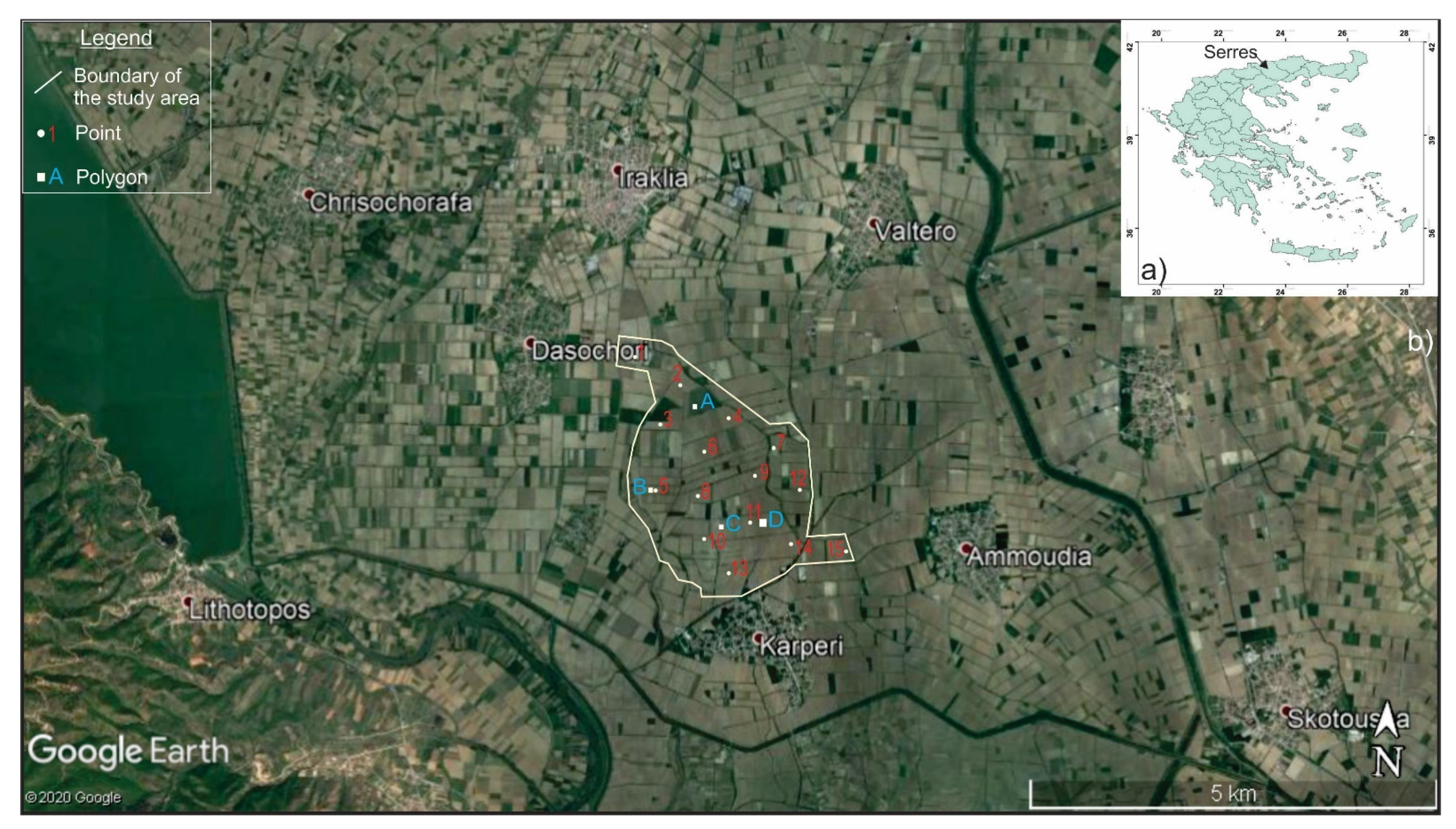
In this paper, we compare both Sentinel-2 and UAV multispectral data from the prefecture of Serres in North Greece (Figure 1) to show how significant the combined use of Sentinel-2 and UAV multispectral data are in precision agriculture.

Specifically, the comparison between the two techniques highlights their advantages and limitations when used in precision agriculture. To address the previous aim, we first computed the NDVI maps of the study area using the QGIS application for both Sentinel-2 and UAV techniques, and further statistically processed the data to reveal the spatiotemporal distribution of the NDVI index. Finally, we conducted both 2D visualization and statistical comparison of the data for both remote sensing techniques.

2. Materials and Methods

2.1. Study Area

The survey area belongs to the prefecture of Serres in North Greece, and it is located near the villages Dasochori and Karperi (41°09′02.75″ N, 23°18′02.63″ E), covering an area of 510 hectares (Figure 1). The area under investigation was cultivated with arable crops (corn, cotton, sunflower, etc.) during the time of this study. This area was selected for the survey because of its high productivity and variability of the crops. The weather conditions were typical for the summer in Greece, characterized by high temperatures and low precipitation. According to the Hellenic National Meteorological Service, the mean temperatures of June, July, August, and September of 2018 were 23.6 °C, 26.2 °C, 27.2 °C and 23.1 °C respectively, while the highest temperatures for these months were 34.7 °C, 36.4 °C, 36.9 °C and 36.8 °C. In addition, the precipitation was 44.0 mm in June, 51.8 mm in July, 17.8 mm in August and 1 mm in September. The maximum temperature exceeded 32 °C for 14 days in June, 23 days in July, 30 days in August, and 12 days in September. Crops have been fully irrigated by a furrow system. The irrigation water comes from the artificial lake of Kerkini, which is located 10 km away from the study area.

2.2. Material and Methods

The image acquisition took part in five different dates from June to October of 2018, partly referred as sensing dates 1, 2, 3, 4, 5 in this study (8 June–12 June 2018, 3 July–6 July 2018, 27 July–28 July 2018, 31 August–1 September 2018, 1 October–3 October 2018, respectively). The period from June to October of 2018 represents a full vegetative season. Two different remote platforms were used for the collection of the images, i.e., Sentinel-2 satellite and the UAV eBee SQ (

Table 1. The bands and their wavelengths for both Sentinel-2 [49] and Parrot Sequoia Plus camera in UAV eBee SQ.

Sensing Platform	Band Number	Band	Central Wavelength (nm)	Bandwith (nm)	Spatial Resolution
Sentinel 2	1	Violet	443	20	60
	2	Blue	490	65	10
	3	Green	560	35	10
	4	Red	665	30	10
	5	Red Edge	705	15	20
	6	Near Infrared	740	15	20
	7		783	20	20
	8		842	115	10
	8b		865	20	20
	9		945	20	60
	10		1380	30	60
	11	Short Wavelength Infrared	1610	90	20
	12		2190	180	20
	Band		Wavelengths (nm)
Sequoia	Green		500–600
	Red		600–700
	Red Edge		700–730
	Near Infrared		700–1300

).

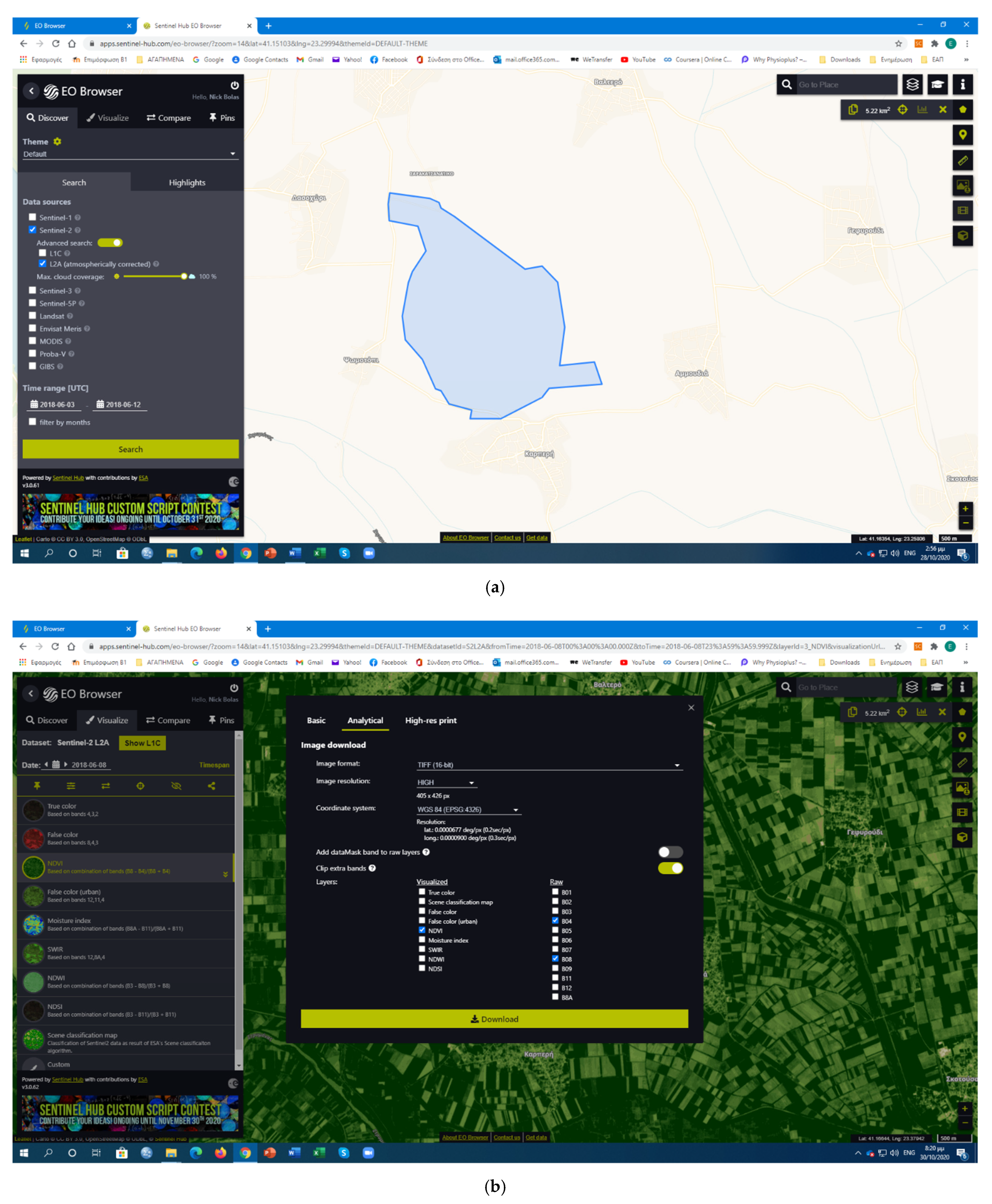
Sentinel-2, implemented by Copernicus European Program for Earth observation, provides high-resolution, multispectral images [48]. The data of Sentinel-2 range from the visible to the shortwave infrared parts of the electromagnetic spectrum with 13 spectral bands at 3 different spatial resolutions depending on the band (10 m, 20 m and 60 m). In this study, the sentinel hub (https://www.sentinel-hub.com/ accessed on 25 March 2021) was used to download the satellite data, corresponding to a spatial resolution of 10 m at ground level since the used bands were B4 and B8 (Figure 2a–c). Also, all images were acquired at processing level 2A. The first Sentinel-2 imagery was collected on 8 June 2018 at 09:28:04 UTC with 0.7% cloudiness, the second on 3 July 2018 at 09:22:24 UTC with 1.9% cloudiness, the third on 28 July 2018 at 09:26:58 UTC with 9.3% cloudiness, the fourth on 1 September 2018 at 09:22:21 UTC with 1.4% cloudiness, and the fifth on 3 October 2018 at 09:26:00 UTC with 5.3% cloudiness.

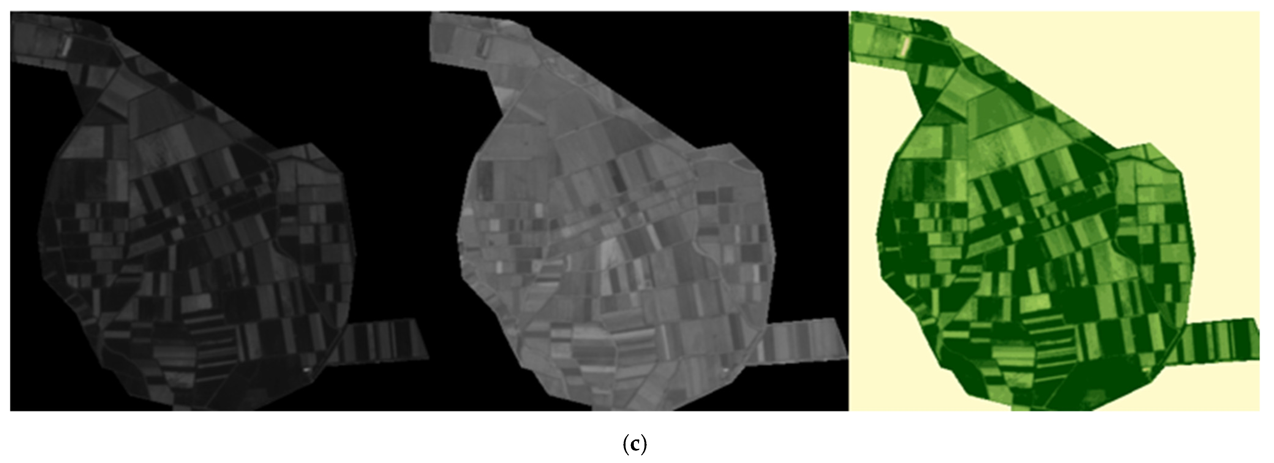
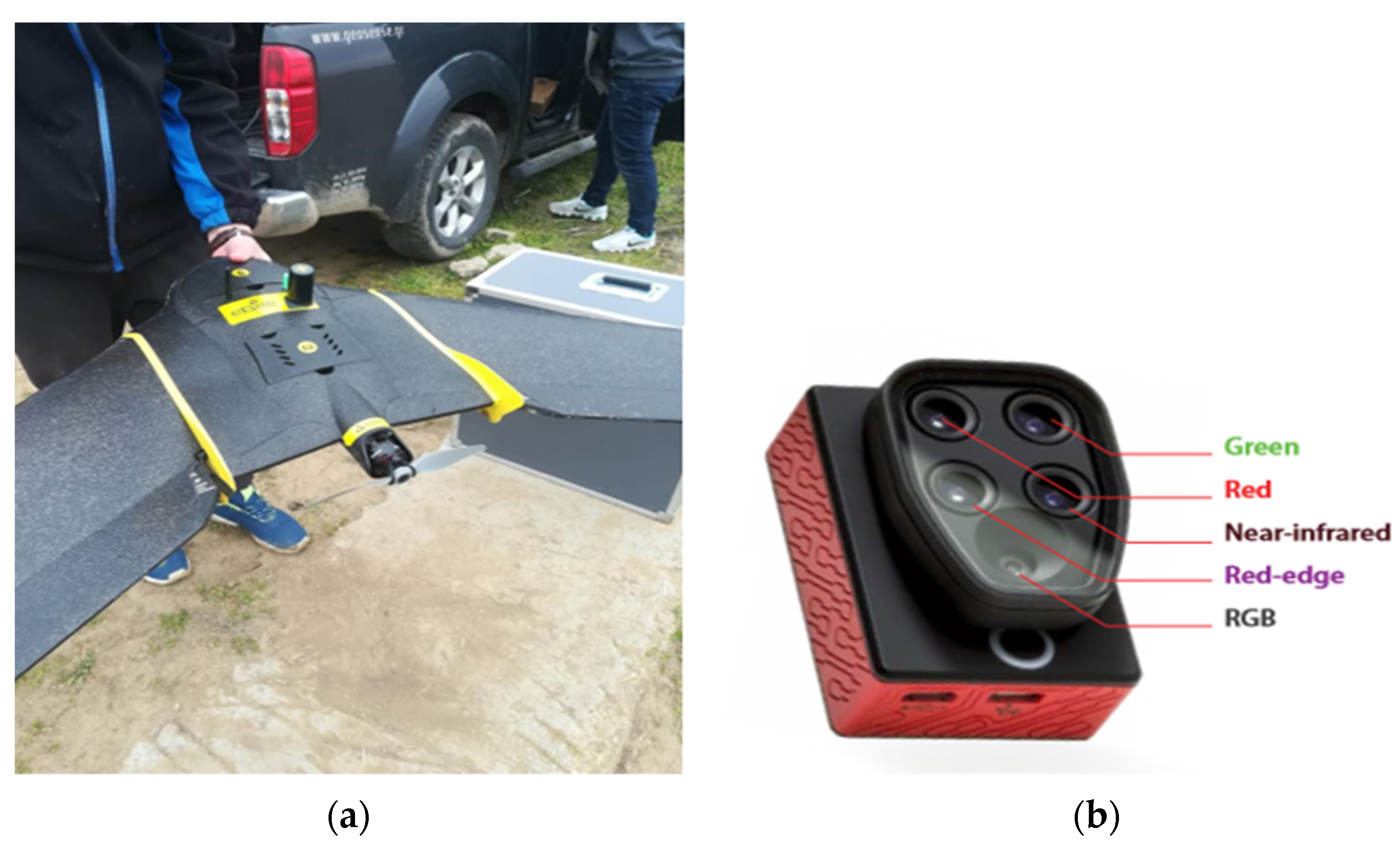
The acquisition of the aerial data has been done by the UAV eBee SQ (Figure 3a,b), equipped with the multispectral camera Parrot Sequoia Plus that corresponds to a spatial resolution of 0.13 m at ground level (Figure 3b). The multispectral sensor consists of four spectral cameras collecting green (530–570 nm), red (640–680 nm), red edge (730–740 nm) and near infrared (NIR) (770–810 nm) imagery (Figure 3b). The campaigns of the UAV were performed on 12 June 2018, on 6 July 2018, on 27 July 2018, on 31 August 2018 and on 3 October 2018. The duration of each campaign was approximately 5–6 h, and the images were collected between 10:00 and 15:00, in clear sky conditions and without wind. The flights were carried out at 120 m height with spatial resolution of 0.13 m (Sequoia sensor). Mapping took part with an average overlap 75% forward and sideways, and 1800 triggers in 4 bands were taken, thus 7,200 multispectral images were acquired. The settings of the sensors were dynamically adjusted to the light conditions during the flights, but they usually worked with F/2.2, 1800 speed, and ISO-100. In addition, we did not resample the UAV images to match the spatial resolution of the satellite imagery aiming to a) keep the initial standards for both platforms, b) show up the discrepancies between the two techniques when applied in field conditions and c) provide an operational view with no dependencies on simultaneous field radiometric sampling, since farmers do not operate resampling in the imagery collected by the drone.

In the context of this survey, the NDVI index was computed and further statistically analyzed for both Sentinel-2 and UAV images (

Table 2. NDVI values of the 15 points of the 5 sensing dates for both the Sentinel-2 and UAV multispectral data.

Sensing Date	8 June 2018– 12 June 2018		3 July 2018– 6 July 2018		27 July 2018– 28 July 2018		31 August 2018– 1 September 2018		1 October 2018– 3 October 2018
Points	Sentinel-2	Sequoia	Sentinel-2	Sequoia	Sentinel-2	Sequoia	Sentinel-2	Sequoia	Sentinel-2	Sequoia
1	0,30878	0,45173	0,77035	0,8728	0,85896	0,90208	0,79467	0,87877	0,49705	0,48634
2	0,25231	0,48002	0,64824	0,71208	0,86481	0,90465	0,82728	0,89512	0,50721	0,447
3	0,24722	0,38731	0,70826	0,82971	0,87684	0,86197	0,84717	0,88098	0,46924	0,46107
4	0,31391	0,32423	0,66333	0,83165	0,84006	0,80724	0,64111	0,83148	0,34081	0,31222
5	0,7164	0,94173	0,83557	0,90238	0,82301	0,86537	0,37613	0,43533	0,25952	0,22123
6	0,71396	0,92676	0,83349	0,91139	0,83356	0,88134	0,36238	0,38788	0,21086	0,22788
7	0,28583	0,54815	0,70521	0,80471	0,85147	0,89067	0,81502	0,8751	0,55524	0,51996
8	0,69419	0,93194	0,8237	0,89235	0,83424	0,87595	0,22414	0,25971	0,28267	0,31891
9	0,39736	0,51542	0,71945	0,85713	0,87891	0,91071	0,78413	0,87402	0,5481	0,48804
10	0,72855	0,85989	0,77669	0,81172	0,38167	0,34895	0,19581	0,19394	0,13616	0,16768
11	0,67647	0,93175	0,83293	0,91139	0,82726	0,88462	0,35944	0,41533	0,21148	0,23982
12	0,30092	0,26731	0,47523	0,61353	0,75925	0,87675	0,79089	0,8238	0,39836	0,44632
13	0,70188	0,93056	0,84293	0,89344	0,82767	0,85523	0,35015	0,36003	0,2318	0,27342
14	0,24646	0,20644	0,22868	0,33886	0,46538	0,53582	0,80488	0,8779	0,76006	0,61152
15	0,39024	0,80005	0,71392	0,89684	0,87108	0,90871	0,83271	0,86174	0,42353	0,42794

). Specifically, the values of the NDVI index were calculated for fifteen points (location in Figure 1b) for every sensing date aiming to find out potential similarities or differences of the index trend between the two platforms (Table 2). The points were chosen randomly within the heterogeneous study area aiming to depict the variability of the area, corresponding to different fields and therefore reflectance. The tool Field Calculator of QGIS application was used for the calculation of the point coordinates, as shown in

Table A1. Coordinates of the points used in the analysis of the present study, as calculated by the Field Calculator tool of QGIS.

Points	Latitude	Longitude
1	41.16315733422939	23.284849229390677
2	41.16000865143369	23.291834238351253
3	41.15581040770609	23.28879413082437
4	41.156606626344086	23.298964014336914
5	41.148354905913976	23.287961720430104
6	41.15262553315412	23.295489605734765
7	41.153132217741934	23.305912831541217
8	41.14770345430107	23.294440044802865
9	41.14991115143369	23.30312606630824
10	41.14285375896058	23.295200071684587
11	41.14488049731183	23.302402231182793
12	41.14839109767025	23.309785349462363
13	41.138981241039424	23.29918116487455
14	41.142564224910394	23.30837387096774
15	41.141695622759855	23.317168467741933

(Appendix A). Additionally, four different parts of the study area (polygons A, B, C, D, location in Figure 1b)) were randomly selected to compute the average NDVI index. The size of the areas, according to the tool Field Calculator of QGIS application, are 1,97076 ha, 3,14675 ha, 4,02501 ha and 6,09571 ha, respectively. The tool Layer Properties of QGIS was used for the calculation of the polygon coordinates, as shown in

Table A2. Coordinates of polygons used in the analysis of the present study, as calculated by the Layer Properties tool of QGIS.

	Coordinates
Polygon	North	South	East	West
A	41.158072392	41.157619996	23.293670970	23.293200477
B	41.148617296	41.148029180	23.282459357	23.287826001
C	41.145260511	41.144618107	23.298412090	23.297670159
D	41.145423374	41.144563819	23.304519449	23.303677991

(Appendix A).

Sentinel-2 imagery acquisition from sentinel hub resulted to the creation of two tiff format images (raw values) corresponding to B04 and B08 bands, along with another one corresponding to the NDVI of the study area for each acquisition date (Figure 2a–c). The two first images were imported into the QGIS application to generate the NDVI map of each Sentinel-2 observation, using the mathematical formula of the index. These NDVI maps were used in the QGIS application for the selection of the fifteen points and the four polygons (A, B, C, D), as well as the calculation of the index values.

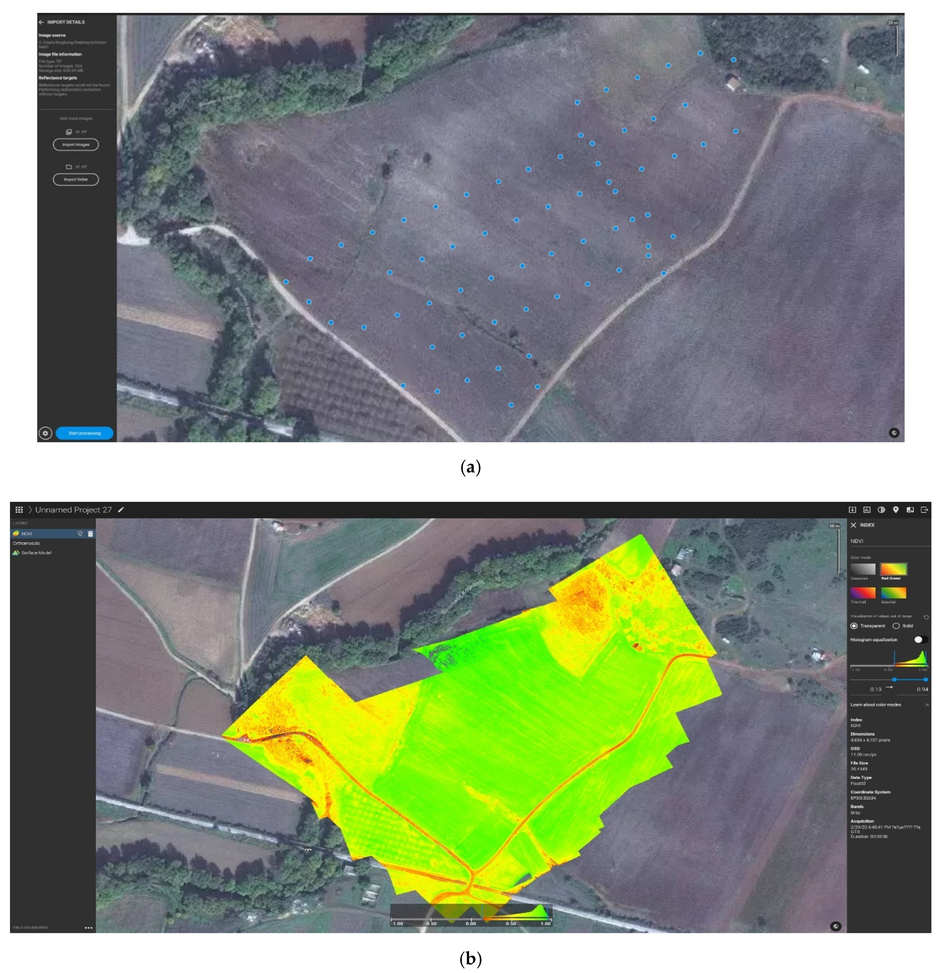
Pix4DFields software was used to carry out the processing of the aerial imagery and the corresponding NDVI map (Figure 4a,b). The software performs a photogrammetric matching of the images and creates reflection values per pixel of the map. The values are calculated according to the number of appearances of each pixel, the camera angle of each appearance and the incident radiation. The process is repeated for the four bands of the sensor (red, red edge, green and near infrared). The user selects the NDVI map generation, and the software creates the corresponding map using the mathematical formula of the index, which is extracted in a tiff format image. A depiction of the index values in color scale can be received as well. QGIS was used to compute the NDVI values of the aerial imagery, as exactly for the Sentinel-2 imagery.

In addition, Minitab software was used to implement the paired-t test for the comparison between the NDVI values of the points. Paired-t test determines whether the means of two dependent groups differ, and it is used to compare measurements that are made for the same items under different conditions. Analysis of variance (ANOVA) was applied to conduct the statistical comparison of the polygon data using Minitab software. Finally, the comparison of the two remote sensing techniques (Sentinel-2 and UAV) for the fifteen different points and the selected parts (polygons A, B, C, D) of the study area in relation with the sensing dates is based on statistical analysis and graphical visualization using charts, graphs, and maps of the mean NDVI values.

3. Results and Discussion

3.1. Distribution of the NDVI Values of Single Points

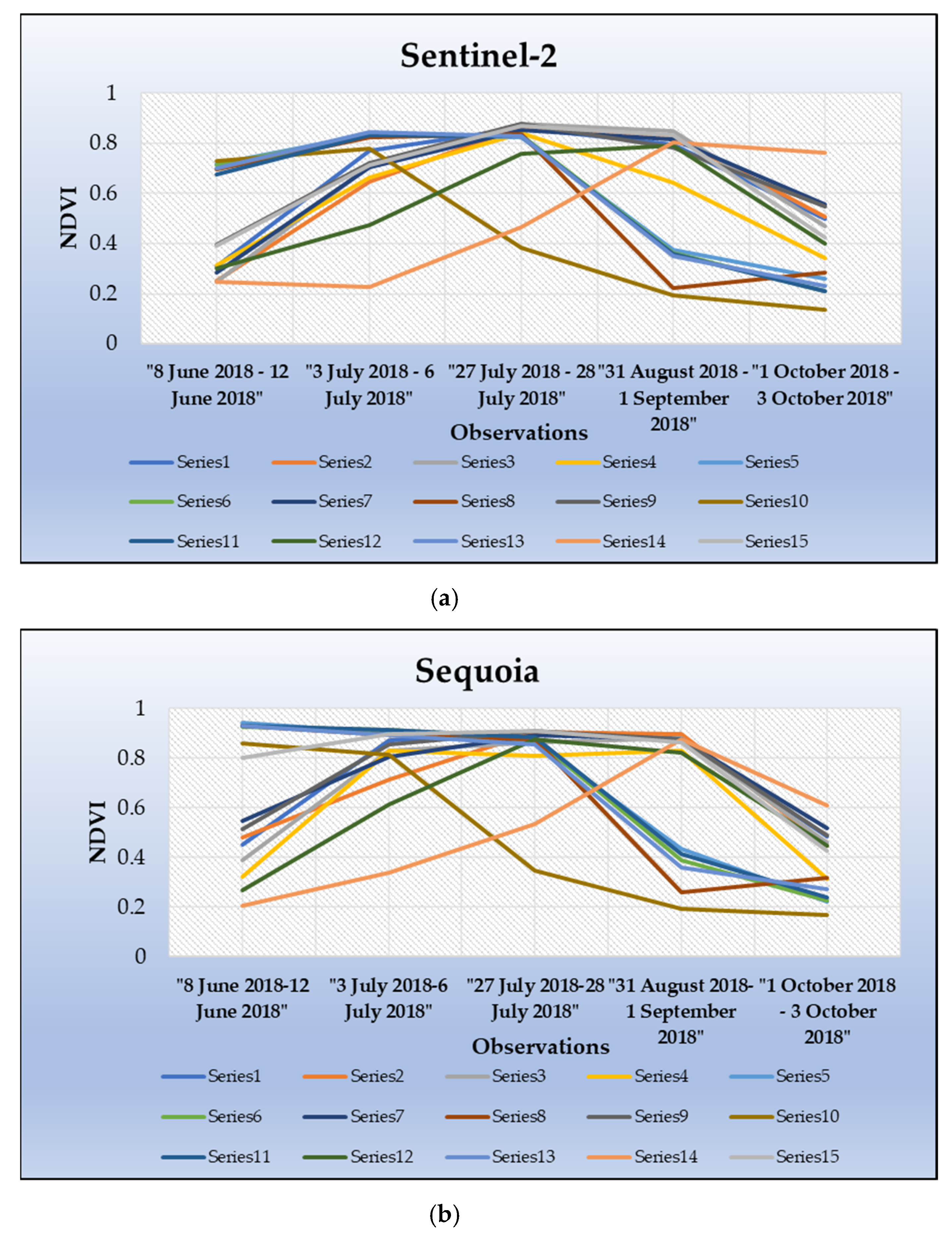
Figure 5a,b presents the distribution of the NDVI values in time for fifteen points (location in Figure 1b) of each sensing date for both Sentinel-2 and UAV images. The fifteen points are randomly distributed in the study area, and this explains the differences in the value range, meaning that each difference corresponds to different crop, thus different plant life cycle and different field even for the same crop, implying spatial management variability. Generally, the charts of Figure 5a,b show a quite similar trend for both techniques. Each line in both graphs of Figure 5 seems to be associated with the sensing dates, taking into consideration the vegetative stages of plant development during the season. Specifically, the first sensing date (8 June–12 June 2018) corresponds to a period related to the vigorous vegetative plant development or to the peak of the development resulting in an increase or in a high-level depiction of the index values. This is clearly shown in most of the lines of both charts. The distribution of the NDVI values presents a stabilization for the next three dates (3 July–6 July 2018, 27 July–28 July 2018, 31 August–1 September 2018) due to the balanced vegetative plant growth occurring from July to September. Finally, the general trend of the NDVI distribution presents a decrease in the last sensing date (1 October–3 October 2018), given that plants are in October at the maturity stage resulting in lower green reflection or they have been harvested resulting in absence of vegetation on the ground.

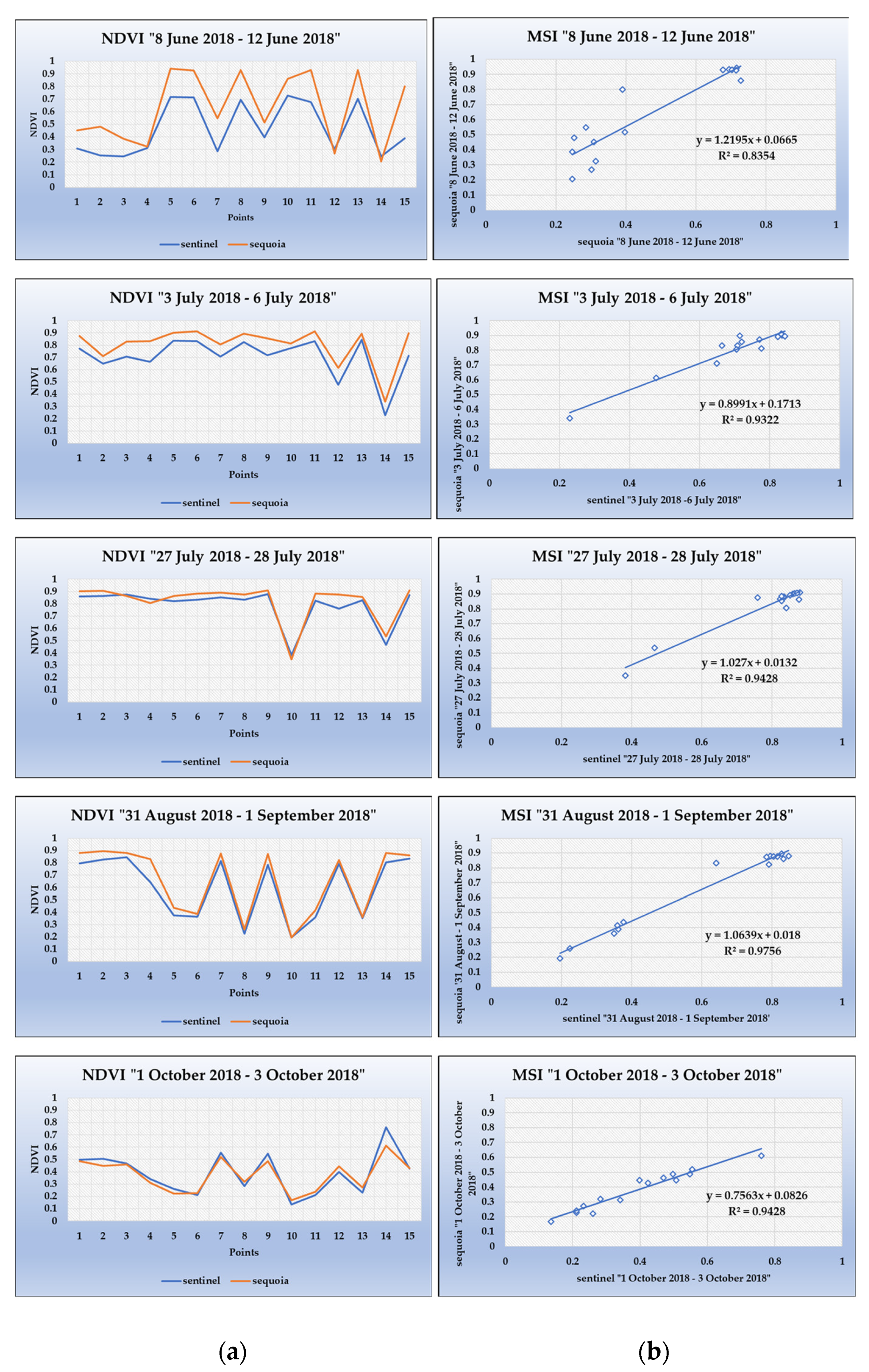
Figure 6a, b presents the distribution of the NDVI values for both the Sentinel-2 and UAV multispectral data, as well as the correlation of these remote sensing techniques for each of the sensing dates. The general trend of the NDVI values is remarkably similar for both techniques (Figure 6a,b). The deviation in the lines of Figure 6a, corresponding to the first and the second sensing dates (8 June–12 June 2018, 3 July–6 July 2018), is probably because of the difference in the plant reflection that decreases as the plant development stage increases. In addition, the scatter charts of Figure 6b show a quite strong linear correlation between the satellite index values and the UAV index values. The correlation coefficient for each sensing date is 83.5%, 93.2%, 94.3%, 97.5% and 94.3%, respectively. The relatively lower correlation coefficient of 83.5%, compared to the rest correlation coefficients that corresponds to the first sensing date (8 June–12 June 2018), is probably related with the early development stage of the plants.

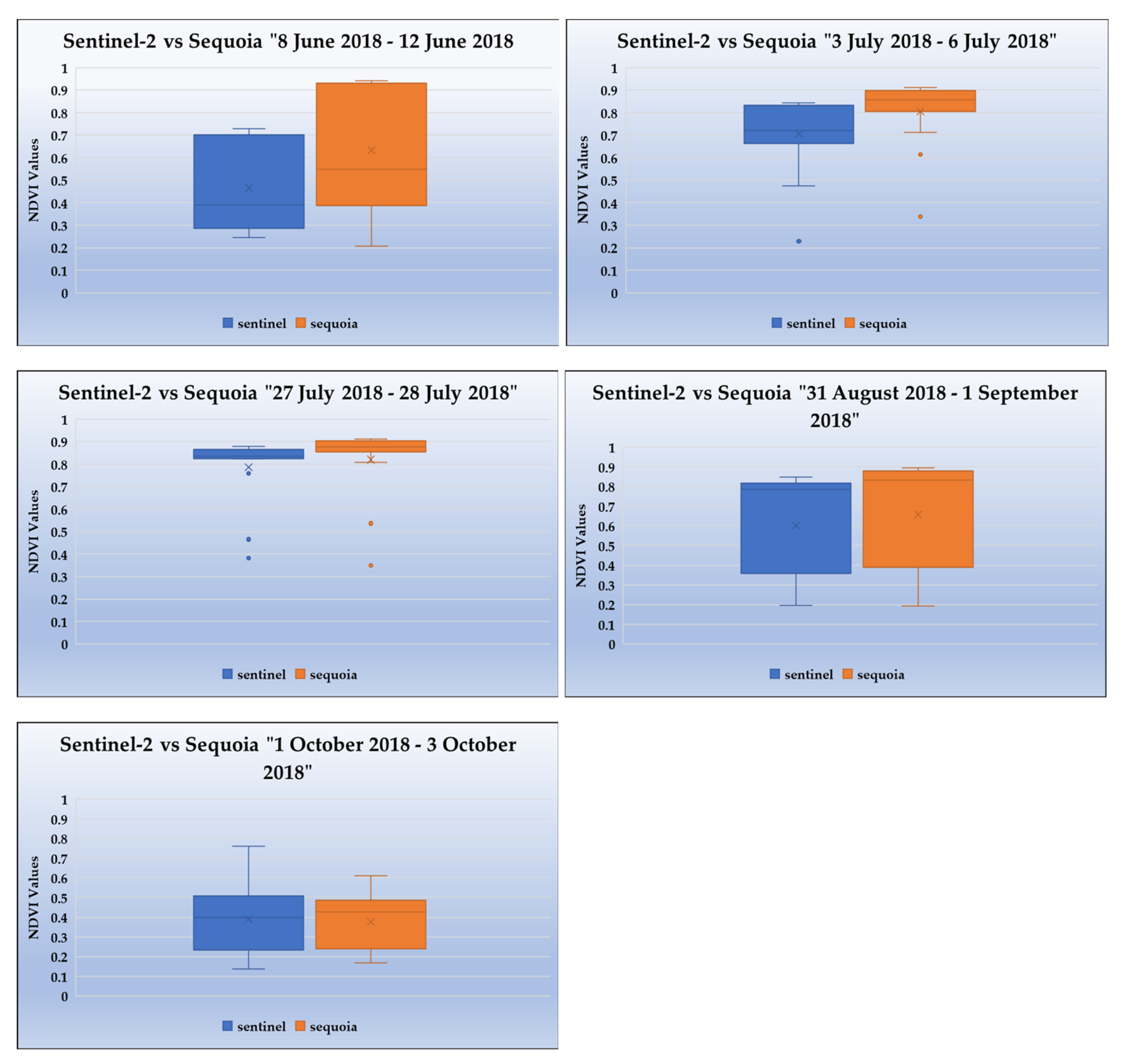
The statistical comparison of the average NDVI of the fifteen points (

Table A3. Statistical analysis of the selected 15 points of the five sensing dates for both Sentinel-2 and UAV multispectral data.

Descriptive Statisticssentinel_1; Sequoia_1; Sentinel_2; … _5; Sequoia_5
Variable	Mean	SE Mean	Standard Deviation	Minimum	Median	Maximum
sentinel_1	0.465	0.0537	0.2079	0.2465	0.3902	0.7286
sequoia_1	0.6336	0.0716	0.2773	0.2064	0.5482	0.9417
sentinel_2	0.7052	0.0424	0.1642	0.2287	0.7195	0.8429
sequoia_2	0.8053	0.0395	0.1529	0.3389	0.8571	0.9114
sentinel_3	0.7863	0.039	0.151	0.3817	0.8342	0.8789
sequoia_3	0.8207	0.0412	0.1597	0.3489	0.8768	0.9107
sentinel_4	0.6004	0.0653	0.2531	0.1958	0.7841	0.8472
sequoia_4	0.6567	0.0704	0.2726	0.1939	0.8315	0.8951
sentinel_5	0.3888	0.044	0.1704	0.1362	0.3984	0.7601
sequoia_5	0.3766	0.0343	0.1327	0.1677	0.4279	0.6115

and

Table A4. Paired-t test of average NDVI values for the fifteen points in five sensing dates.

Observation	Descriptive Statistics					Estimation for Paired Difference				Test
						µ_Difference: Mean of (Sentinel-2–Sequoia)				Null Hypothesis H₀: μ_Difference = 0 Alternative Hypothesis H₁: μ_Difference ≠ 0
	Sample	N	Mean	StDev	SE Mean	Mean	StDev	SE Mean	95% CI for μ_Difference	T-Value	p-Value
8 June 2018–12 June 2018	sentinel-2	15	0.465	0.2079	0.0537	−0.1686	0.1214	0.0314	(−0.2358; −0.1013)	−5.38	0.000
	sequoia	15	0.6336	0.2773	0.0716
3 July 2018– 6 July 2018	sentinel-2	15	0.7052	0.1642	0.0424	−0.1001	0.0431	0.0111	(−0.1240; −0.0763)	−9	0.000
	sequoia	15	0.8053	0.1529	0.0395
27 July 2018–28 July 2018	sentinel-2	15	0.7863	0.151	0.039	−0.0344	0.03843	0.00992	(−0.05567; −0.01311)	−3.47	0.004
	sequoia	15	0.8207	0.1597	0.0412
31 August 2018–1 September 2018	sentinel-2	15	0.6004	0.2531	0.0653	−0.0563	0.0455	0.0118	(−0.0816; −0.0311)	−4.79	0.000
	sequoia	15	0.6567	0.2726	0.0704
1 October 2018–3 October 2018	sentinel-2	15	0.3888	0.1704	0.044	0.0122	0.0523	0.0135	(−0.0168; 0.0411)	0.9	0.382
	sequoia	15	0.3766	0.1327	0.0343

in Appendix A) for the two remote sensing techniques is based on the paired-t test taking into consideration the assumption of its implementation (independence of observations, normality of the distribution of the residuals and the equality of variances). The analysis showed statistical significance between the averages of the index of the two remote sensing techniques for the first 4 sensing dates (8 June–12 June 2018, 3 July–6 July 2018, 27 July–28 July 2018, 31 August–1 September 2018) since the P values of the paired t-test are very low (<0.05). This is not the case for the last date (1 October–3 October 2018), where the P value of the test is higher than 0.05. The boxplots of Figure 7 confirm that the average NDVI index of the fifteen points corresponding to the first four sensing dates is higher for the NDVI derived by the UAV multispectral data. This is because of the higher spatial resolution of the Sequoia camera.

3.2. Distribution of the NDVI for the Selected Polygons (A, B, C, D)

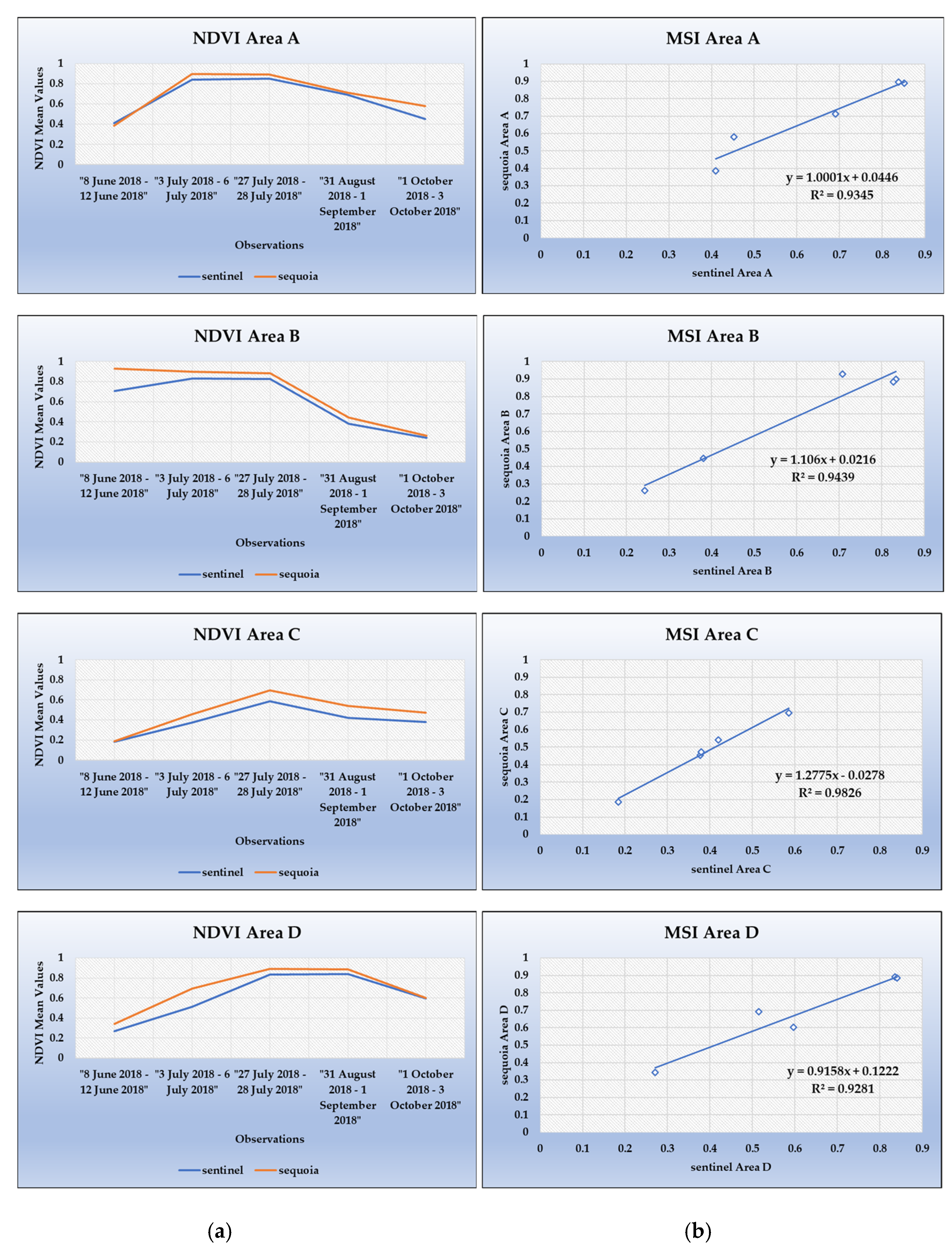
Figure 8a,b presents the distribution of the average NDVI values within the selected polygons (A, B, C, D, location in Figure 1b) of each sensing date for both Sentinel-2 and UAV images. The line charts of Figure 8a demonstrate an almost identical trend in the distribution of the average NDVI for both remote sensing techniques. The vegetative stages of plant development (increase, stabilization, decrease) are also observed as exactly in Figure 5a that presents the distribution of the NDVI for the fifteen selected points. The scatter charts of Figure 8b show a strong linear correlation between the data for both remote sensing techniques, which is confirmed for every sensing date. The correlation coefficient for each sensing date is 93.45%, 94.39%, 98.26% and 92.81% respectively.

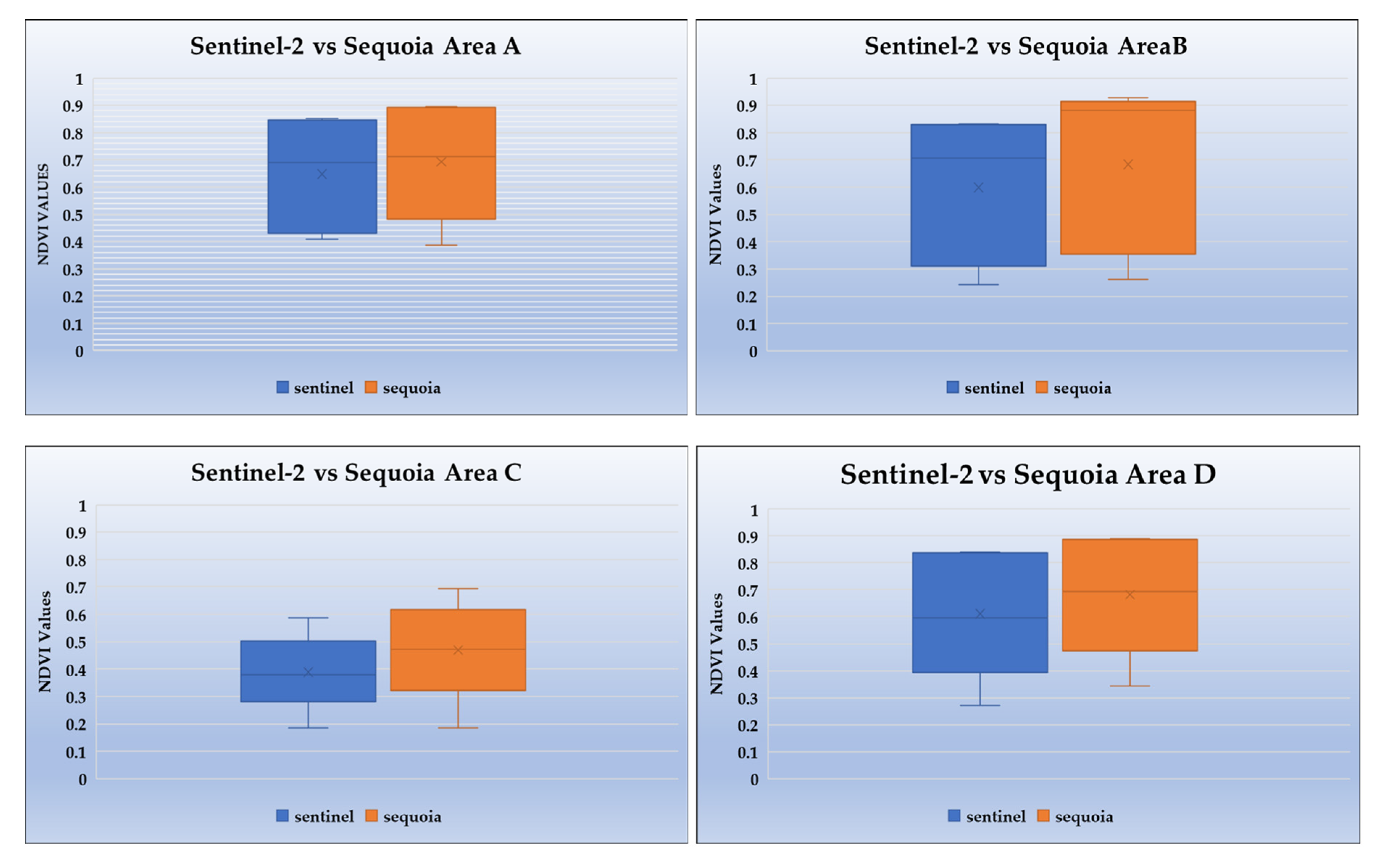
The ANOVA model (

Table A5. Statistical analysis of the selected areas (polygons A, B, C, D) for satellite and aerial imagery, as computed by QGIS. STDDEV is for standard deviation and CV for coefficient of variability.

Area	Platform	Sensing Date	MAX	MEAN	MIN	STDDEV	CV
A	Sentinel-2	8 June 2018–12 June 2018	0.424764931	0.409668865	0.398896009	0.00590227	1.44%
	Sentinel-2	3 July 2018–6 July 2018	0.842377245	0.838002589	0.83181119	0.002107325	0.25%
	Sentinel-2	27 July 2018–28 July 2018	0.862135291	0.851049562	0.828952312	0.009149611	1.08%
	Sentinel-2	31 August 2018–1 September 2018	0.703845322	0.690205042	0.657489479	0.009797661	1.42%
	Sentinel-2	1 October 2018–3 October 2018	0.466080695	0.451860976	0.419669837	0.011385355	2.52%
	Sequoia	8 June 2018–12 June 2018	0.739971459	0.386712345	0.267078608	0.039826689	10.30%
	Sequoia	3 July 2018–6 July 2018	0.918028831	0.896014414	0.840995193	0.008689196	0.97%
	Sequoia	27 July 2018–28 July 2018	0.920731068	0.888997866	0.685243845	0.019670044	2.21%
	Sequoia	31 August 2018–1 September 2018	0.856916368	0.712623024	0.432811826	0.062304516	8.74%
	Sequoia	1 October 2018–3 October 2018	0.776085019	0.579790769	0.353510261	0.065478958	11.29%
B	Sentinel-2	8 June 2018–12 June 2018	0.72285974	0.707651934	0.6915797	0.008361191	1.18%
	Sentinel-2	3 July 2018–6 July 2018	0.840008736	0.833387507	0.822145224	0.00401236	0.48%
	Sentinel-2	27 July 2018–28 July 2018	0.843239069	0.827542223	0.805931032	0.007401045	0.89%
	Sentinel-2	31 August 2018–1 September 2018	0.426836431	0.38117364	0.349979818	0.017986821	4.72%
	Sentinel-2	1 October 2018–3 October 2018	0.292903215	0.24251502	0.214875594	0.018805529	7.75%
	Sequoia	8 June 2018–12 June 2018	0.957545161	0.929184155	0.725212157	0.01313116	1.41%
	Sequoia	3 July 2018–6 July 2018	0.931631625	0.898681251	0.770359695	0.011027217	1.23%
	Sequoia	27 July 2018–28 July 2018	0.927700162	0.882190463	0.694832087	0.017135325	1.94%
	Sequoia	31 August 2018–1 September 2018	0.731545687	0.445202932	0.280894756	0.045929647	10.32%
	Sequoia	1 October 2018–3 October 2018	0.607119501	0.262282414	0.174537793	0.043217779	16.48%
C	Sentinel-2	8 June 2018–12 June 2018	0.206350893	0.184016948	0.163822144	0.009934681	5.40%
	Sentinel-2	3 July 2018–6 July 2018	0.579889655	0.377094243	0.176204428	0.095115443	25.22%
	Sentinel-2	27 July 2018–28 July 2018	0.772020161	0.585997589	0.290901035	0.096564769	16.48%
	Sentinel-2	31 August 2018–1 September 2018	0.492080986	0.41989237	0.315348059	0.049551697	11.80%
	Sentinel-2	1 October 2018–3 October 2018	0.591126442	0.379471433	0.214191154	0.121058057	31.90%
	Sequoia	8 June 2018–12 June 2018	0.802700639	0.185702369	0.121396981	0.056253917	30.29%
	Sequoia	3 July 2018–6 July 2018	0.89239186	0.455740255	0.101822048	0.236436583	51.88%
	Sequoia	27 July 2018–28 July 2018	0.902240813	0.694348733	0.130899876	0.191690991	27.61%
	Sequoia	31 August 2018–1 September 2018	0.868877113	0.539666935	0.16559723	0.140022944	25.95%
	Sequoia	1 October 2018–3 October 2018	0.85949403	0.472400034	0.164854422	0.180505956	38.21%
D	Sentinel-2	8 June 2018–12 June 2018	0.290092528	0.270967551	0.248297825	0.010585632	3.91%
	Sentinel-2	3 July 2018–6 July 2018	0.602515101	0.515073871	0.366025954	0.065445929	12.71%
	Sentinel-2	27 July 2018–28 July 2018	0.869380832	0.835450653	0.770878434	0.026236285	3.14%
	Sentinel-2	31 August 2018–1 September 2018	0.856839776	0.840226661	0.822994411	0.006889503	0.82%
	Sentinel-2	1 October 2018–3 October 2018	0.72909236	0.596489981	0.524814963	0.055854803	9.36%
	Sequoia	8 June 2018–12 June 2018	0.73825258	0.342425083	0.18140173	0.099854429	29.16%
	Sequoia	3 July 2018–6 July 2018	0.903458595	0.691964177	0.192108214	0.150160703	21.70%
	Sequoia	27 July 2018–28 July 2018	0.9346416	0.890634058	0.378713846	0.042593657	4.78%
	Sequoia	31 August 2018–1 September 2018	0.927322805	0.883830221	0.603708208	0.013481126	1.53%
	Sequoia	1 October 2018–3 October 2018	0.81042999	0.602571672	0.282279491	0.084460655	14.02%

and

Table A6. ANOVA for the NDVI means of the selected areas (polygons A, B, C, D) in five sensing dates (from left to right).

ANOVA: NDVI_MEAN versus Sensing Platforms; Observations
Areas	Factor Information				Analysis of Variance for NDVI_MEAN_Areas						Model Summary
	Factor	Type	Levels	Values	Source	DF	SS	MS	F	P	S	R-sq	R-sq(adj)
A	Sensing Platforms	Fixed	2	Sentinel-2; Sequoia	Sensing Platform	1	0.00499	0.00499	3.26	0.145	0.0390	0.983	0.962
	Observations	Fixed	5	1,2,3,4,5	Observations	4	0.35492	0.08873	58.07	0.001
					Error	4	0.00611	0.00153
					Total	9	0.36602
B	Sensing Platforms	Fixed	2	Sentinel-2; Sequoia	Sensing Platform	1	0.01809	0.01809	5.87	0.073	0.0555	0.982	0.959
	Observations	Fixed	5	1,2,3,4,5	Observations	4	0.66153	0.16538	53.68	0.001
					Error	4	0.01232	0.00308
					Total	9	0.69194
C	Sensing Platforms	Fixed	2	Sentinel-2; Sequoia	Sensing Platform	1	0.01611	0.01611	14.84	0.018	0.0329	0.981	0.958
	Observations	Fixed	5	1,2,3,4,5	Observations	4	0.21389	0.05347	49.24	0.001
					Error	4	0.00434	0.00109
					Total	9	0.23434
D	Sensing Platforms	Fixed	2	Sentinel-2; Sequoia	Sensing Platform	1	0.01248	001248	6.08	0.069	0.0453	0.981	0.958
	Observations	Fixed	5	1,2,3,4,5	Observations	4	0.42572	0.10643	51.83	0.001
					Error	4	0.00821	0.00205
					Total	9	0.44641

in Appendix A), that is used to compare the NDVI index means of the Sentinel-2 and UAV multispectral data, indicated statistical significance only between the NDVI mean of polygon C (P value of the ANOVA lower than 0.05) and no statistical significance for the rest of the polygons (P values of the ANOVA tests higher than 0.05). This is probably due to the high spatial variability of the area corresponding to polygon C, as shown by its higher coefficient of variability (CV) (Table A5 in Appendix A). This is also confirmed by the optical visualization of the NDVI means for both techniques, shown in the boxplots of Figure 9. The boxplots show that the NDVI means of the data, acquired by Sequoia camera, are higher compared to those acquired by Sentinel-2 for polygon C and slightly higher for polygons A, B and D (even without statistical significance). In addition, the range of the NDVI values (max, min, mean, standard deviation, coefficient of variability) is larger for the data collected by the UAV compared to those collected from Sentinel-2. This is due to the higher spatial resolution of the UAV that enables the more accurate identification of the vegetative alteration (higher index values).

3.3. 2D Visualization of the Sentinel-2 and UAV Multispectral Data

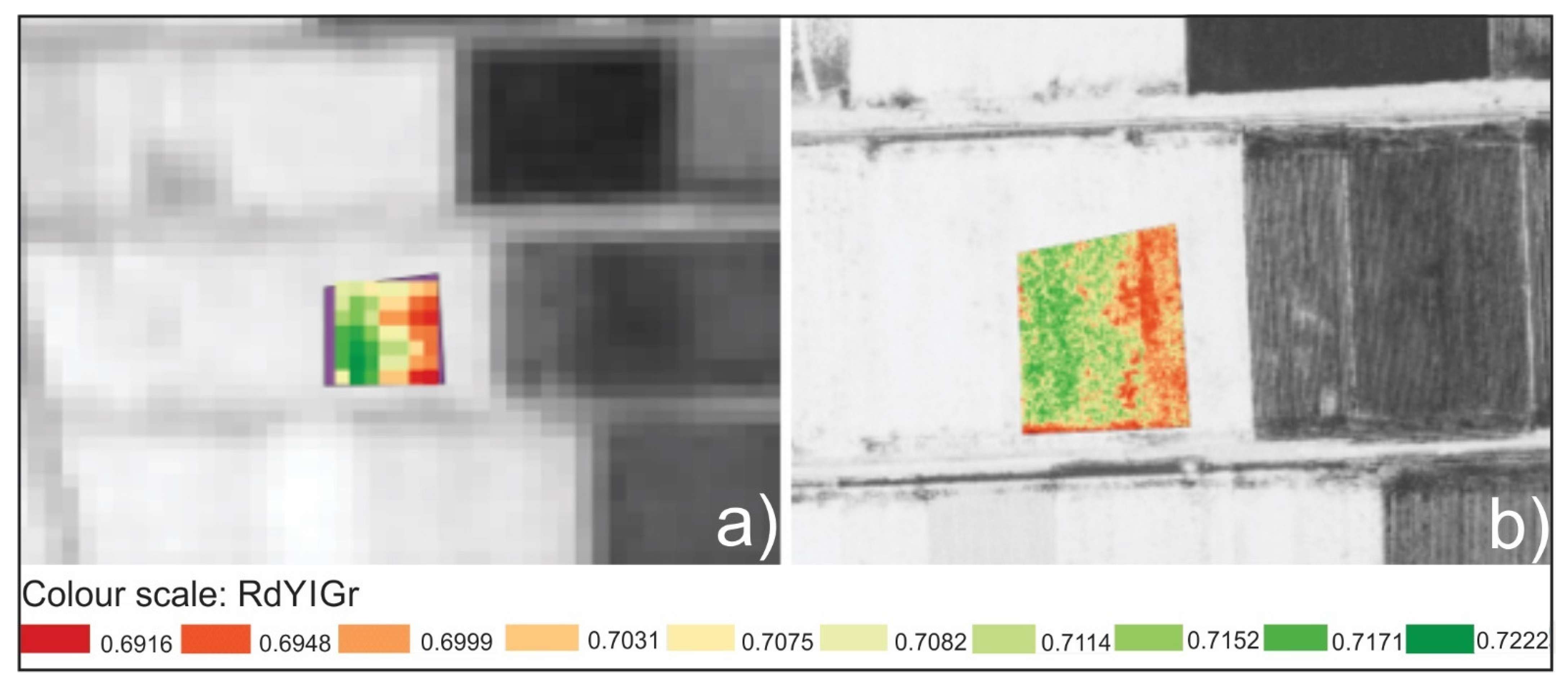
The 2D visual comparison of the two remote sensing techniques (Sentinel-2 and UAV) is facilitated by the false colored display of the data of the first sensing date for polygon B (location in Figure 1) in scale 1:1000 using QGIS software (Figure 10a,b). The high density of vegetation on the left side of polygon B and the gradual decrease in vegetation from left to right are visible in both images (Figure 10a,b). Moreover, the higher resolution of sequoia camera (Figure 10b) enables the detection of the lower density parts even on the left side of polygon B, or the identification of barren parts on the ground. In other words, sequoia camera visualizes more effectively how dense is the vegetation making available a more detailed escalation of the vegetation density (Figure 10b). The ability of the multispectral camera of the UAV to be more analytic and effective compared to the satellite’s sensor is evident.

3.4. The Use of Sentinel-2 and UAV Multispectral Data in Precision Agriculture

It is evident in this research, supported by similar works [50,51,52,53,54,55,56,57,58], that both Sentinel-2 and UAV techniques sufficiently manage to image the overall state (health, alteration) of the existing vegetation, as well as the vegetative stages (increase, stabilization, decrease) during the season (Figure 5, Figure 6, Figure 7, Figure 8 and Figure 9). However, the multispectral sensor of the UAV can provide more details about the density of the vegetation due to its higher spatial resolution (Figure 10).

The spatial extent of the study area is a very important factor associated with the efficient use of the two techniques. For example, Sequoia camera in this research has a clear advantage over the satellite sensor when it is used to provide information for a specific point or a small area on the ground. Thus, this advantage gradually reduces as the spatial extent of the study area increases (Figure 9). This is because the NDVI mean value is affected by higher values when the spatial extent of the study area increases.

Furthermore, important parameters that can impact the decision to select one of the two monitoring techniques are the cost, the aim of the monitoring and the requirements of the area to be imaged. The cost of the UAV imagery includes the purchase cost of the vehicle equipped with the multispectral camera, the purchase cost of the software for aerial imagery processing, and the expenditures for the pilot’s license. Nevertheless, all these costs constantly decrease over years. In addition, the physical presence of the UAV user in the field implies extra time and cost, as well as limitations related to the extent of the study area. However, the physical presence of the UAV user is valuable since there is access to specific data for each site in the field, such as slopes, weeds, plant population, etc. To the opposite, the use of Sentinel-2 data is easier and cheaper for the study of vegetation’s general characteristics in extensive areas and without the physical presence of staff.

Considering previous works [50,51,52,53,54,55,56,57,58] and the present one, we report the following:

• The use of Sentinel-2 platform is proved effective to describe the vegetation and the vigority of the plants presenting a quite similar behavior to the UAVs’ data regarding the NDVI trend.
• Sentinel-2 imagery does not always manage to detect localized conditions, especially in areas showing high heterogeneity due to abiotic or biotic stress. In such cases, the use of UAV is necessary.

In summary, we recommend the combined use of both remote sensing techniques being the optimum solution in precision agriculture. This is because Sentinel-2 provides the cost-effective information regarding the general characteristics of the vegetation, while UAVs data are more analytic in case of localized operations, such as fertilization and phytosanitary applications.

4. Conclusions

In this study, imagery of the sentinel-2 satellite is compared with imagery of an UAV equipped with multispectral camera, aiming to evaluate both techniques based on the NDVI index.

The statistical comparison between Sentinel-2 and UAV imagery shows that:

• The trend of the average NDVI is almost identical for both remote sensing techniques.
• There is a strong correlation of the NDVI index between the two techniques.
• Four out of five observations indicated statistical significance for the mean values of the NDVI index for the fifteen points, with the UAV multispectral data to present the higher ones. Considering the polygons, one polygon from the four showed statistical significance of the NDVI mean between the techniques.
• The range of the NDVI values (max, min) is larger and the coefficient of variability (CV) is higher for the UAV multispectral data compared to Sentinel-2 data due to the higher spatial resolution of the UAV’s sensor.
• The multispectral camera of the UAV is recommended for localized operations because it is more analytic and effective compared to the satellite’s sensor.

In conclusion, both UAV and Sentinel-2 platforms provide important information for the vegetation cover of the Earth’s surface, and they are important tools for the precision agriculture system. The choice of the most appropriate technology (UAV or satellite) depends on the use and the aim of the data collection, as they have different spatial analysis, cost, and requirements. Satellite imagery is a valuable tool when we need information for areas of large extent to further select and focus on specific fields of interest, according to the requirements of our survey. Nevertheless, UAV technique is a better choice when detailed information for the study area is required.

References

- Pinter, P.J.; Hatfield, J.L.; Schepers, J.S.; Barnes, E.M.; Moran, M.S.; Daughtry, C.S.T.; Upchurch, D.R. Remote Sensing for Crop Management. Photogramm. Eng. Remote Sens. 2003, 69, 647–664. [Google Scholar] [CrossRef] [Green Version]
- Gomarasca, M.A. Basics of Geomatics, 1st ed.; Springer: Dordrecht, The Netherlands, 2009. [Google Scholar] [CrossRef]
- Ravelo, A.C.; Abril, E.G. Remote Sensing. In Applied Agrometeorology; Stigter, K., Ed.; Springer: Berlin/Heidelberg, Germany, 2010; pp. 1013–1024. [Google Scholar] [CrossRef]
- Jones, H.G.; Vaughan, R.A. Remote Sensing of Vegetation Principles, Techniques, and Applications; Oxford University Press: Oxford, UK, 2010; ISBN 9780199207794. [Google Scholar]
- Kingra, P.K.; Majumder, D.; Singh, S.P. Application of Remote Sensing and GIS in Agriculture and Natural Resource Management Under Changing Climatic Conditions. Agric. Res. J. 2016, 53, 295–302. [Google Scholar] [CrossRef]
- Mani, J.K.; Varghese, A.O. Remote Sensing and GIS in Agriculture and Forest Resource Monitoring. In Geospatial Technologies in Land Resources Mapping, Monitoring and Management, Geotechnologies and the Environment, 1st ed.; Reddy, G., Singh, S., Eds.; Springer International Publishing: Cham, Switzerland, 2018; Volume 21, pp. 377–400. [Google Scholar] [CrossRef]
- Shanmugapriya, P.; Rathika, S.; Ramesh, T.; Janaki, P. Applications of Remote Sensing in Agriculture—A Review. Int. J. Curr. Microbiol. App. Sci. 2019, 8, 2270–2283. [Google Scholar] [CrossRef]
- Strickland, R.M.; Ess, D.R.; Parsons, S.D. Precision Farming and Precision Pest Management: The Power of New Crop Production Technologies. J. Nematol. 1998, 30, 431–435. [Google Scholar]
- Singh, A.K. Precision Farming; I.A.R.I.: New Delhi, India, 2001. [Google Scholar]
- Robert, P.C. Precision agriculture: A challenge for crop nutrition management. Plant Soil 2002, 247, 143–149. [Google Scholar] [CrossRef]
- Zhang, M.; Li, M.Z.; Liu, G.; Wang, M.H. Yield Mapping in Precision Farming. In Computer and Computing Technologies in Agriculture, Volume II. CCTA 2007. The International Federation for Information Processing; Li, D., Ed.; Springer: Boston, MA, USA, 2007; Volume 259, pp. 1407–1410. [Google Scholar] [CrossRef] [Green Version]
- Goswami, S.B.; Matin, S.; Saxena, A.; Bairagi, G.D. A Review: The application of Remote Sensing, GIS and GPS in Precision Agriculture. Int. J. Adv. Technol. Eng. Res. 2012, 2, 50–54. [Google Scholar]
- Heege, H.J.; Thiessen, E. Sensing of Crop Properties. In Precision in Crop Farming: Site Specific Concepts and Sensing Methods: Applications and Results; Heege, H., Ed.; Springer Science + Business Media: Dordrecht, The Nenderlands, 2013; pp. 103–141. [Google Scholar] [CrossRef]
- Zude-Sasse, M.; Fountas, S.; Gemtos, T.A.; Abu-Khalaf, N. Applications of precision agriculture in horticultural crops. Eur. J. Hortic. Sci. 2016, 81, 78–90. [Google Scholar] [CrossRef]
- Balafoutis, A.; Beck, B.; Fountas, S.; Vangeyte, J.; van der Wal, T.; Soto, I.; Gomez-Barbero, M.; Barnes, A.; Eory, V. Precision Agriculture Technologies Positively Contributing to GHG Emissions Mitigation, Farm Productivity and Economics. Sustainability 2017, 9, 1339. [Google Scholar] [CrossRef] [Green Version]
- Paustian, M.; Theuvsen, L. Adoption of precision agriculture technologies by German crop farmers. Precis. Agric. 2017, 18, 701–716. [Google Scholar] [CrossRef]
- Pallottino, F.; Biocca, M.; Nardi, P.; Figorilli, S.; Menesatti, P.; Costa, C. Science mapping approach to analyse the research evolution on precision agriculture: World, EU and Italian situation. Precis. Agric. 2018, 19, 1011–1026. [Google Scholar] [CrossRef]
- Fulton, J.; Hawkins, E.; Taylor, R.; Franzen, A. Yield Monitoring and Mapping. In Precision Agriculture Basics; Shannon, D.K., Clay, D.E., Kitchen, N.R., Eds.; ASA, CSSA, SSSA: Madison, WI, USA, 2018; pp. 63–77. [Google Scholar] [CrossRef]
- Shafi, U.; Mumtaz, R.; García-Nieto, J.; Hassan, S.A.; Zaidi, S.A.R.; Iqbal, N. Precision Agriculture Techniques and Practices: From Considerations to Applications. Sensors 2019, 19, 3796. [Google Scholar] [CrossRef] [PubMed] [Green Version]
- Nandibewoor, A.; Hebbal, S.B.; Hegadi, R. Remote Monitoring of Maize Crop through Satellite Multispectral Imagery. Procedia Comput. Sci. 2015, 45, 344–353. [Google Scholar] [CrossRef] [Green Version]
- Escola, A.; Badia, N.; Arno, J.; Martinez-Casanovas, J.A. Using Sentinel-2 images to implement Precision Agriculture techniques in large arable fields: First results of a case study. Adv. Anim. Biosci. 2017, 8, 377–382. [Google Scholar] [CrossRef] [Green Version]
- Belgiu, M.; Csillik, O. Sentinel-2 cropland mapping using pixel-based and object-based time-weighted dynamic time warping analysis. Remote Sens. Environ. 2018, 204, 509–523. [Google Scholar] [CrossRef]
- Ahmad, L.; Mahdi, S.S. Satellite Farming; Springer International Publishing: Cham, Switzerland, 2018; ISBN 978-3-030-03448-1. [Google Scholar] [CrossRef]
- Rapinel, S.; Mony, C.; Lecoq, L.; Clément, B.; Thomas, A.; Hubert-Moy, L. Evaluation of Sentinel-2 time-series for mapping floodplain grassland plant communities. Remote Sens. Environ. 2019, 223, 115–129. [Google Scholar] [CrossRef]
- Zhang, C.; Kovacs, J.M. The application of small unmanned aerial systems for precision agriculture: A review. Precis. Agric. 2012, 13, 693–712. [Google Scholar] [CrossRef]
- Anderson, K.; Gaston, K.J. Lightweight unmanned aerial vehicles will revolutionize spatial ecology. Front. Ecol. Environ. 2013, 11, 138–146. [Google Scholar] [CrossRef] [Green Version]
- Csillik, O.; Cherbini, J.; Johnson, R.; Lyons, A.; Kelly, M. Identification of Citrus Trees from Unmanned Aerial Vehicle Imagery Using Convolutional Neural Networks. Drones 2018, 2, 39. [Google Scholar] [CrossRef] [Green Version]
- Barbedo, J.G. A Review on the Use of Unmanned Aerial Vehicles and Imaging Sensors for Monitoring and Assessing Plant Stresses. Drones 2019, 3, 40. [Google Scholar] [CrossRef] [Green Version]
- Mesas-Carrascosa, F.J.; Notario-Garcia, M.D.; de Larriva, J.E.M.; de la Orden, M.S.; Garcia-Ferrer Porras, A. Validation of measurements of land plot area using UAV imagery. Int. J. Appl. Earth Obs. Geoinf. 2014, 33, 270–279. [Google Scholar] [CrossRef]
- Rokhmana, C.A. The potential of UAV-based remote sensing for supporting precision agriculture in Indonesia. Procedia Environ. Sci. 2015, 24, 245–253. [Google Scholar] [CrossRef] [Green Version]
- Yun, G.; Mazur, M.; Pederii, Y. Role of Unmanned Aerial Vehicles in Precision Farming. Proc. Natl. Aviat. Univ. 2017, 10, 106–112. [Google Scholar] [CrossRef]
- Manfreda, S.; McCabe, M.E.; Miller, P.E.; Lucas, R.; Madrigal, V.P.; Mallinis, G.; Dor, E.B.; Helman, D.; Estes, L.; Ciraolo, G.; et al. On the Use of Unmanned Aerial Systems for Environmental Monitoring. Remote Sens. 2018, 10, 641. [Google Scholar] [CrossRef] [Green Version]
- Maes, W.H.; Steppe, K. Perspectives for Remote Sensing with Unmanned Aerial Vehicles in Precision Agriculture. Trends Plant. Sci. 2019, 24, 152–164. [Google Scholar] [CrossRef]
- Radoglou-Grammatikis, P.; Sarigiannidis, P.; Lagkas, T.; Moscholios, I. A compilation of UAV applications for precision agriculture. Comput. Netw. 2020, 172, 107148. [Google Scholar] [CrossRef]
- Ozdarici-Ok, A. Automatic detection and delineation of citrus trees from VHR satellite imagery. Int. J. Remote Sens. 2015, 36, 4275–4296. [Google Scholar] [CrossRef]
- Pérez-Ortiz, M.; Peña, J.M.; Gutiérrez, P.A.; Torres-Sánchez, J.; Hervás-Martínez, C.; López-Granados, F. A semi-supervised system for weed mapping in sunflower crops using unmanned aerial vehicles and a crop row detection method. Appl. Soft. Comput. 2015, 37, 533–544. [Google Scholar] [CrossRef]
- Torres-Sánchez, J.; López-Granados, F.; Peña, J.M. An automatic object-based method for optimal thresholding in UAV images Application for vegetation detection in herbaceous crops. Comput. Electron. Agric. 2015, 114, 43–52. [Google Scholar] [CrossRef]
- Panagiotakis, C.; Kokinou, E. Unsupervised Detection of Topographic Highs with Arbitrary Basal Shapes Based on Volume Evolution of Isocontours. Comput. Geosci. 2017, 102, 22–33. [Google Scholar] [CrossRef]
- De Castro, A.I.; Torres-Sánchez, J.; Peña, J.M.; Jiménez-Brenes, F.M.; Csillik, O.; López-Granados, F. An automatic random forest-OBIA algorithm for early weed mapping between and within crop rows using UAV imagery. Remote Sens. 2018, 10, 285. [Google Scholar] [CrossRef] [Green Version]
- Georgi, C.; Spengler, D.; Itzerott, S.; Kleinschmit, B. Automatic delineation algorithm for site-specific management zones based on satellite remote sensing data. Precis. Agric. 2018, 19, 684–707. [Google Scholar] [CrossRef] [Green Version]
- Louargant, M.; Jones, G.; Faroux, R.; Paoli, J.-N.; Maillot, T.; Gée, C.; Villette, S. Unsupervised classification algorithm for early weed detection in row-crops by combining spatial and spectral information. Remote Sens. 2018, 10, 761. [Google Scholar] [CrossRef] [Green Version]
- Haboudane, D.; Miller, J.R.; Tremblay, N.; Zarco-Tejada, P.J.; Dextraze, L. Integrated narrowband vegetation indices for prediction of crop chlorophyll content for application to precision agriculture. Remote Sens. Environ. 2002, 81, 416–426. [Google Scholar] [CrossRef]
- Tarnavsky, E.; Garrigues, S.; Brown, M.E. Multiscale geostatistical analysis of AVHRR, SPOT-VGT, and MODIS global NDVI products. Remote Sens. Environ. 2008, 112, 535–549. [Google Scholar] [CrossRef]
- Anderson, J.H.; Weber, K.T.; Gokhale, B.; Chen, F. Intercalibration and Evaluation of ResourceSat-1 and Landsat-5 NDVI. Can. J. Remote Sens. 2011, 37, 213–219. [Google Scholar] [CrossRef]
- Simms, É.L.; Ward, H. Multisensor NDVI-Based Monitoring of the Tundra-Taiga Interface (Mealy Mountains, Labrador, Canada). Remote Sens. 2013, 5, 1066–1090. [Google Scholar] [CrossRef] [Green Version]
- Houborg, R.; McCabe, M.F. High-Resolution NDVI from planet’s constellation of earth observing nano-satellites: A new data source for precision agriculture. Remote Sens. 2016, 8, 768. [Google Scholar] [CrossRef] [Green Version]
- Fawcett, D.; Panigada, C.; Tagliabue, G.; Boschetti, M.; Celesti, M.; Evdokimov, A.; Biriukova, K.; Colombo, R.; Miglietta, F.; Rascher, U.; et al. Multi-Scale Evaluation of Drone-Based Multispectral Surface Reflectance and Vegetation Indices in Operational Conditions. Remote Sens. 2020, 12, 514. [Google Scholar] [CrossRef] [Green Version]
- European Space Agency. Sentinel-2 User Handbook; European Space Agency: Paris, France, 2015; pp. 53–54. [Google Scholar]
- Fletcher, K. Sentinel-2. ESA’s Optical High-Resolution Mission for GMES Operational Services; ESA Communications: Noordwijk, The Netherlands, 2012; ISBN 978-92-9221-419-7. [Google Scholar]
- Ünsalan, C.; Boyer, K.L. (Eds.) Remote Sensing Satellites and Airborne Sensors. In Multispectral Satellite Image Understanding. Advances in Computer Vision and Pattern Recognition; Springer: London, UK, 2011; pp. 7–15. [Google Scholar] [CrossRef]
- Matese, A.; Toscano, P.; Di Gennaro, S.F.; Genesio, L.; Vaccari, F.P.; Primicerio, J.; Belli, C.; Zaldei, A.; Bianconi, R.; Gioli, B. Intercomparison of UAV, aircraft and satellite remote sensing platforms for precision viticulture. Remote Sens. 2015, 7, 2971–2990. [Google Scholar] [CrossRef] [Green Version]
- McCabe, M.F.; Houborg, R.; Lucieer, A. High-resolution sensing for precision agriculture: From Earth-observing satellites to unmanned aerial vehicles. Remote Sens. Agric. Ecosyst. Hydrol. XVIII 2016, 9998, 999811. [Google Scholar]
- Benincasa, P.; Antognelli, S.; Brunetti, L.; Fabbri, C.A.; Natale, A.; Sartoretti, V.; Modeo, G.; Guiducci, M.; Tei, F.; Vizzari, M. Reliability of Ndvi Derived by High Resolution Satellite and Uav Compared To in-Field Methods for the Evaluation of Early Crop N Status and Grain Yield in Wheat. Exp. Agric. 2017, 54, 1–19. [Google Scholar] [CrossRef]
- Borgogno-Mondino, E.; Lessio, A.; Tarricone, L.; Novello, V.; de Palma, L. A comparison between multispectral aerial and satellite imagery in precision viticulture. Precis. Agric. 2018, 19, 195. [Google Scholar] [CrossRef]
- Malacarne, D.; Pappalardo, S.E.; Codato, D. Sentinel-2 Data Analysis and Comparison with UAV Multispectral Images for Precision Viticulture. GI Forum 2018, 105–116. [Google Scholar]
- Khaliq, A.; Comba, L.; Biglia, A.; Ricauda Aimonino, D.; Chiaberge, M.; Gay, P. Comparison of Satellite and UAV-Based Multispectral Imagery for Vineyard Variability Assessment. Remote Sens. 2019, 11, 436. [Google Scholar] [CrossRef] [Green Version]
- Pla, M.; Bota, G.; Duane, A.; Balagué, J.; Curcó, A.; Gutiérrez, R.; Brotons, L. Calibrating Sentinel-2 Imagery with Multispectral UAV Derived Information to Quantify Damages in Mediterranean Rice Crops Caused by Western Swamphen (Porphyrio porphyrio). Drones 2019, 3, 45. [Google Scholar] [CrossRef] [Green Version]
- Messina, G.; Peña, J.M.; Vizzari, M.; Modica, G. A Comparison of UAV and Satellites Multispectral Imagery in Monitoring Onion Crop. An Application in the ’Cipolla Rossa di Tropea’ (Italy). Remote Sens. 2020, 12, 3424. [Google Scholar] [CrossRef]
Figure 1.
(a) Map of Greece from Google Earth showing the prefecture of Serres where (b) the survey area (white polygon) of this work is located. The fifteen different points and the four different parts of the study area (polygons A, B, C, D) used for the comparison of the Sentinel-2 and UAV multispectral data are also shown.
Figure 2.
Sentinel-2 images used in the present work: (a) selection of the studied area, acquisition mode (L2A) and sensing dates in the sentinel hub, (b) NDVI map and NDVI value calculation, (c) from left to right Sentinel-2_L2A_B04_(Raw), Sentinel-2_L2A_B08_(Raw) and Sentinel-2 L2A_NDVI.
Figure 3.
The eBee SQ (a) and the multispectral camera Parrot Sequoia Plus (b) used to acquire the UAV images of this work.
Figure 4.
UAV images used in the present work: (a) Processing of the aerial imagery by PIX4DFields software, (b) NDVI map from UAV multispectral data produced by the PIX4DFields software.
Figure 5.
Distribution of the NDVI values for the 15 pixels for both (a) Sentinel-2 and (b) UAV multispectral data (Sequoia). Generally, the charts show a quite similar trend for both remote sensing techniques.
Figure 6.
(a) distribution of the NDVI values for both Sentinel-2 and UAV multispectral data (Sequoia) for each of the sensing dates, (b) correlation of the remote sensing techniques for each of the sensing dates. The general trend of the NDVI values is remarkably similar for both techniques, and the correlation coefficients are generally strong.
Figure 7.
Boxplots of average NDVI values for the fifteen points, showing that the average NDVI index of the fifteen points corresponding to the first four sensing dates is higher for the NDVI derived by the UAV multispectral data, probably due to the higher spatial resolution of the Sequoia camera.
Figure 8.
(a) Distribution of the NDVI values of the four selected polygons (A, B, C, D, location in Figure 1) for both the Sentinel-2 and UAV multispectral data (Sequoia) (b) correlation of the remote sensing techniques. The general trend of the NDVI values is remarkably similar for both techniques, and the correlation coefficients are generally strong.
Figure 9.
Boxplots of the NDVI mean values for the four selected polygons (A, B, C, D, location in Figure 1). The boxplots show that the NDVI means of the data, acquired by Sequoia camera, are higher compared to those acquired by Sentinel-2 for polygon C and slightly higher for polygons A, B and D.
Figure 10.
A 2D visualization of area B (location in Figure 1, N′ 41,148617296, S′ 41,14802918, E′ 23,282459357, W′ 23,287826001) of the first observation (8 June 2018–12 June 2018) based on (a) Sentinel-2 data and (b) UAV multispectral data in scale 1:1000 and in color scale RdYlGr. The ability of the multispectral camera of the UAV to be more analytic and effective compared to the satellite’s sensor is evident.