Multi-Step Short-Term Wind Speed Prediction Using a Residual Dilated Causal Convolutional Network with Nonlinear Attention

Abstract

Wind energy is the most used renewable energy worldwide second only to hydropower. However, the stochastic nature of wind speed makes it harder for wind farms to manage the future power production and maintenance schedules efficiently. Many wind speed prediction models exist that focus on advance neural networks and/or preprocessing techniques to improve the accuracy. Since most of these models require a large amount of historic wind data and are validated using the data split method, the application to real-world scenarios cannot be determined. In this paper, we present a multi-step univariate prediction model for wind speed data inspired by the residual U-net architecture of the convolutional neural network (CNN). We propose a residual dilated causal convolutional neural network (Res-DCCNN) with nonlinear attention for multi-step-ahead wind speed forecasting. Our model can outperform long-term short-term memory networks (LSTM), gated recurrent units (GRU), and Res-DCCNN using sliding window validation techniques for 50-step-ahead wind speed prediction. We tested the performance of the proposed model on six real-world wind speed datasets with different probability distributions to confirm its effectiveness, and using several error metrics, we demonstrated that our proposed model was robust, precise, and applicable to real-world cases.

1. Introduction

With increasing concern about global warming and pollution caused by over usage of fossil fuels, the leading world organizations and countries are encouraging renewable energy sources like wind and solar power. According to the U.S. Energy Information Administration, renewable energy contributes to over 18% of total energy production with solar and wind energy contributing almost 10% [1]. Wind energy is mostly generated at on-shore or off-shore clusters of wind turbines also known as wind farms. These wind farms in order to manage the future production of total electrical power efficiently require prior knowledge of future wind conditions. We can classify the wind speed prediction problem into several temporal ranges. According to [2], there are four temporal ranges for forecasting: (1) long-term, with a range of a week to a year or much ahead; (2) medium-term, for two days to a week ahead; (3) short-term, for one hour to two days ahead; (4) very short-term, from a few seconds to one hour. Accurate short-term prediction is used for economic load dispatch planning, such as increase and decrease in wind power supply and is used to preplan distribution from the wind farms. Short-term wind speed prediction is also vital for advanced scheduling of the cleaning, maintenance, and safety check of wind turbines during low-wind conditions.

Generally, numerical and statistical approaches are used to predict wind speed. Numerical models require a large amount of historical multivariate data of terrain to make accurate forecasts; also, large processing power is required to assemble such a method, thus not being recommended for short-term forecasting [3]. Statistical approaches consider the relationship between input and output data to create a prediction model. Conventional statistical methods proposed by Jenkins [4] can be categorized as follows: autoregressive mode (AR), moving average model (MA), autoregressive moving average (ARMA), and auto-regressive integrated moving average model (ARIMA). ARIMA models are used to predict and model high-frequency wind speed data. In [5], the authors proposed a nested ARIMA model that uses non-stationary features of wind speed data for forecasting and generates surrogate data for wind speed. In [6], a stochastic differential equation approach (Langevin model) was used to model the normal behavior of wind turbine towers’ vibration using wind speed using high-frequency sampling data. This method outperformed the deterministic neural network (NN) methods for high frequency data; however, the authors also suggested that NN models are just as good for 10 min sampling time series.

Several studies also used artificial intelligence models such as neural networks for the wind prediction problems. In [7], the author used a back-propagation (BP) algorithm to train a neural network on two previous wind speed data points to predict the next wind speed data point, which outperformed statistical models in terms of prediction accuracy. The work in [8] used a complex-valued recurrent neural network (RNN) to train the model on a complex wind speed signal (wind speed + wind direction) to perform multi-step ahead predictions. In [9], the authors proposed a linear model for predicting one-day-ahead wind speed and direction by developing a linear model and using the least-squares method for parameter estimation. These studies confirmed that wind speed can be predicted by using historical data in the absence of a numerical model that requires several environmental variables such as the pressure gradient, air temperature, and orography. In [10], the results also confirmed the assumption that one can train a model only using historical data and still get reasonable accuracy. Using a different approach, the work in [11] used a hybrid approach by combining the numerical model with a Gaussian process-based probabilistic model. The authors applied a Gaussian process model to the wind speed data output of the numerical weather model (NWP) to make one-day-ahead wind power forecast.

In more recent studies, the research has been focused on finding better neural network architectures to improve the wind speed prediction accuracy. Many of these focused on the aspects of deep learning or advanced preprocessing techniques. In [12], principal component analysis (PCA) was used to reduce the input dimension and search the optimal input sample size for the deep-LSTM architecture. This architecture combined with PCA achieved better accuracy compared to support vector machines (SVM), the back-propagation neural network (BPNN), and the LSTM model without PCA analysis. This model was validated using the classic training and testing split method, also known as the holdout method [13,14], where they trained the model on a part of a historic dataset and validated the performance on another. Using the SVM regression method combined with the evolutionary algorithm, the work in [15] presented a novel approach for hyperparameter estimation of SVM models using evolutionary programming (EP) and particle swarm optimization (PSO), which in turn outperformed a multi-layer perceptron (MLP)-based regression model. The training and testing split of data was 80% and 20%, respectively, and training set was divided into 10 subsets. In a similar research proving the capabilities of LSTM, the work in [16] presented the results showing that the LSTM model could outperform SVM while predicting wind speed using multiple environmental attributes like previous wind speed, pressure, relative humidity, temperature, and solar radiation. While this study showed very supporting results for LSTM, also claiming that the requirement of training data was low, the study did not explain the training procedure of these models. Some studies used advanced preprocessing or data preparation methods. In [17], targeted and adjacent wind turbines with related time-lag characteristics were exploited using wavelet coherence transformation analysis (WCT) preceded by continuous wavelet transformation (CWT) to establish the spatial-temporal correlation. An LSTM model was trained on the CWT of wind speed signals, which clearly outperformed the conventional BP, extreme learning machine (ELM), and SVM models. Models in this research were trained and tested on a data split of training, validation, and testing sets. In general, the LSTM model is very popular for wind speed prediction. The work in [18] introduced a modification to the LSTM structure to better predict the weather contextual data and decrease the naive character of generic LSTM. By introducing an adaptive compression algorithm, cell regulation, and rectified linear units (ReLU) units to generic LSTM, the improved model was able to increase the prediction accuracy for wind power. The model was validated using an 80% training split and 20% testing split. Discrete wavelet transformation (DWT) was used as a data preprocessing method in [19], and several LSTMs were trained on the z-score normalized values of different decomposition levels of the DWT of the original wind signal. The z-score denormalized values of each predicted value for each decomposition level were added to get the final prediction. The DWT method was also tested with recurrent neural networks (RNN), BP, generic LSTM, RNN, and BP with a training, validation, and testing set of 70%, 20%, and 10%, respectively. The models were optimized using Adam, a first-order optimization algorithm. Results confirmed that the LSTM model trained with DWT decompositions performed better than the rest of the models on short-term prediction of wind speed. The deep learning method proposed in [20] used the wavelet packet decomposition, CNN, and CNN-LSTM models for wind speed prediction. A hybrid model was reported in [21], by incorporating the double decomposition and error correction with the LSTM model to improve one-step-ahead prediction of short-term wind speed. In [22], the authors used different configurations of artificial neural networks (ANN) to predict the hourly wind speed time series. In a different approach, ELM with kernel mean p-power error loss [23] was used to improve the wind speed prediction accuracy. The author claimed that ELM based on second-order statistics was not suitable for a non-linear and non-Gaussian dataset, so a new loss function was introduced, and PCA was applied to reduce some of the redundant data components. In a more recent paper [24], a direct multi-step-ahead prediction model was by combining LSTM with ensemble empirical model decomposition (EEMD) and fuzzy entropy and compared against the SVM, BP, and generic LSTM models. Another ensemble forecasting method based on a multi-objective optimization algorithm was proposed in [25] for wind speed forecasting that included the back-propagation neural network (BPNN), RBF, general regression neural networks (GRNN), and the wavelet neural network (WNN) with singular spectrum analysis for data preprocessing.

Since most of the recent research for wind related prediction is focused on the LSTM-based architecture or improving the traditional models, another type of machine learning architecture known as the convolutional neural network (CNN) is also an alternative for time series forecasting. Unlike LSTM or the conventional model, CNN requires little to no data preprocessing. The work in [26] introduced a 1D CNN-based forecasting model for direct multi-step-ahead prediction for short-term wind speed data. The model was trained on 75% of the dataset and tested on 25% and outperformed the SVM, radial function (RF), decision tree (DT), and MLP models on 11 datasets. Apart from wind speed prediction, CNN architectures have traditionally been used in time series classification. In [27], it was shown that the CNN model could extract a suitable internal structure to produce deep features automatically and outperform state-of-the-art methods on real-world datasets. CNN architectures, unlike other feature-based models, do not require sophisticated feature engineering [28,29,30]. These papers provided supportive results and reviews showing that 1D CNN could be used as an automatic feature extraction mechanism for one-dimensional data. Several studies have presented the innovations in CNN to improve its suitability for time series data. Some hybrid models of the CNN architecture with the gated recurrent unit (GRU) are also used for wind speed predictions. In [31], a CNN-GRU model was introduced for short-term wind prediction that used CNN as a feature extraction method for multivariate weather data and then fed the features to the GRU model to make predictions. A model called the dilated causal convolutional neural network (DCCNN), also known as the deep temporal convolutional network (DTCN), has been used in multiple time series applications, including multivariate prediction [32], real-time water level prediction [33], and seismic event prediction [34]. Moving a step further, WaveNet was proposed in [35], a network comprised of the residual unit of DCCNN for raw audio generation. Another CNN architecture, widely used in medical image segmentation, is called U-net. U-net is named after its U-shaped structure, where low-level features are fused with high-level features to learn cross-context information. The works in [36,37] gave us an insight into the success of U-net in image segmentation. Attention modules are sometimes also used to improve the performance of U-nets. The works in [38,39,40] propose attention modules for U-net architectures in medical image applications.

The application of attention modules in time series models is also an active field of research. The works in [41,42] proposed the application of attention in the LSTM architecture for time series prediction. Attention models have also been used with CNN and time series data. The work in [43] proposed an attention gated CNN for sentence classification, and the work in [44] introduced a temporal causal discovery framework (TCDF) for learning causal relationships in time series data. However, many innovative CNN architectures mentioned above have not yet been explored for renewable energy applications. Studies are often focused on learning linear causal relationships from training data.

We exploited the time series feature extraction power of DCCNN and the computational efficiency with the low data requirement of U-net to discover the complex underlying relationship in time series wind speed signals. We used a nonlinear attention module to merge the low-level features of residual DCCNN U-net (ResUnet) to high-level features. We used a sliding window training method to train our models, using eight hours of wind speed data with a sampling frequency of 10 min to predict the next eight hours’ wind speed. We also compared our model against the naive prediction method, LSTM, GRU, residual DCCNN (SeriesNet), and residual DCCNN U-net (ResUnet) architectures. In summary,

• We present “ResAUnet”, a residual dilated convolutional network based on U-net that uses nonlinear attention to merge the causal features of low-level residual blocks with high-level residual blocks to learn the nonlinear causal relationship in wind speed data for short-term wind prediction.
• We evaluate the performance of our proposed model and several other time series prediction models on six real-world wind speed datasets with different probability distributions using multiple time series error metrics.

We organize the remainder of this paper as follows. Section 2 presents the details of LSTM, GRU, residual dilated CNN, ResUnet, and the proposed model (ResAUnet). It also provides detailed information of the hyperparameters used for each model. In Section 2.6, we describe the wind speed dataset used for the evaluation of the model. Section 3 presents the model training method used in the presented research and the performance metrics used for the accuracy comparison of different models. We detail the results of this research at the end of Section 3. Conclusions of this study are given in Section 4.

2. Prediction Models and Method

In this section, we describe the different wind speed prediction models used for benchmarking, as well as the proposed model. We start with the brief introduction of LSTM, GRU, DCCNN, and attention. Then, we move on to the details of the proposed model.

2.1. Long-Term Short-Term Memory and Gated Recurrent Unit

Long-term short-term memories (LSTM) are a variation of RNN modules introduced to overcome the long-term dependencies problem of RNN. LSTM, introduced by [45], are capable of learning long-term dependencies and are used by state-of-the-art time series prediction models. The concept behind the LSTM model is a memory cell that maintains its state over time and non-linear forgetting units that regulate the information in and out of the memory cell. In order to utilize all the information present in the time series data, the dataset is normally chronologically arranged before feeding into LSTM.

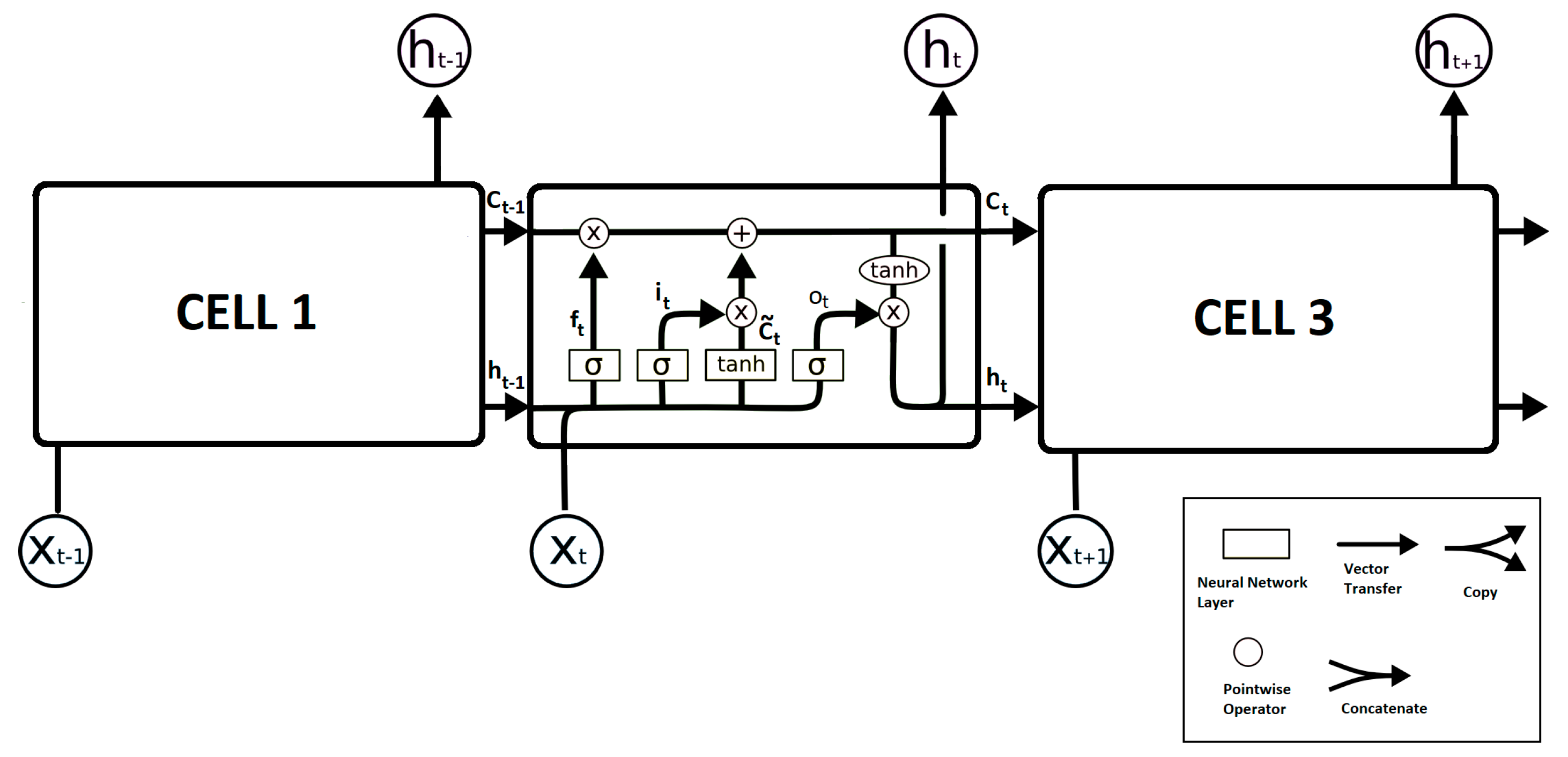
Figure 1 shows the structure of an LSTM network, where every cell’s output, also known as the control state, h, is connected to the next cell’s input, x. The cell state C is also shared with the next LSTM cell in the chain. An LSTM cell contains an input gate, i, which decides the information originating from the new observation at current timestep t, and the output of the previous timestep t-1 will be stored in the unit state or not. Then, a forget gate, f, selectively forgets some of the past trends and other time series factors. Later, the output gate, o, determines the output and cell state for the current timestep observation. All the gates have their separate weight matrix, W, and bias vector, b. The training process of LSTM can be written as the following equations.

$$i_t=\sigma \left(W_i·\left[h_{t-1},x_t\right]+b_i\right)$$

(1)

$$f_t=\sigma \left(W_f·\left[h_{t-1},x_t\right]+b_f\right)$$

(2)

$${\tilde{C}}_t=tanh\left(W_C·\left[h_{t-1},x_t\right]+b_C\right)$$

(3)

$$C_t=f_t\odot C_{t-1}+i_t\odot {\tilde{C}}_t$$

(4)

$$o_t=\sigma \left(W_o·\left[h_{t-1},x_t\right]+b_0\right)$$

(5)

$$h_t=o_t\odot \tanh (C_t)$$

(6)

In the above equations, the $\odot$operator represents the Hadamard product [46], also known as element-wise multiplication of two matrices. In Equations (1), (2), and (5), σ represents a sigmoid activation. Similarly, in Equations (3) and (6), tanh represents a hyperbolic tangent activation. The equations for the sigmoid and hyperbolic tangent activations are as follows.

$$\mathsf{\sigma }\left(\mathrm{x}\right)=\frac{e^x}{\left(1+e^x\right)}$$

(7)

$$\tanh \left(x\right)=1-\frac{2}{1+e^{-2x}}$$

(8)

The length of the LSTM chain can be determined by the length of the output/prediction steps. A fully-connected (FC) layer follows the LSTM chain to output step temporal features. The equation for each neuron in an FC layer with linear activation can be written as follows.

$$y_k={{\displaystyle \sum }}_{i=0}^m{w}_{ki}{x}_i$$

(9)

where $y_k$ is the output of the k^th neuron, $x_i$ is the i^th input x, $w_{ki}$ is the weight for the i^th input, and m is the total number of input variables. The FC layer at the end of the LSTM chain finds the complex relationship between the LSTM outputs and training variables to further improve the accuracy of the architecture. The model used for comparison in this paper uses the backpropagation algorithm for training. The backpropagation algorithm is also known as the backpropagation of errors [47] and is a chain rule method. Using an optimizer (often, a gradient-based one), after each forward pass through the network, the algorithm applies a backward pass to adjust the model’s parameters, such as weights and biases. For the LSTM architecture, we made use of the first-order gradient-based stochastic objective optimization algorithm, Adam [48]. The name of the Adam optimization algorithm is derived from adaptive moment estimation because it uses estimations of the first and second moments of the gradient to adapt/adjust the learning rate for each weight of the neural network. For more details on how the Adam optimization works, one may refer to the referenced paper.

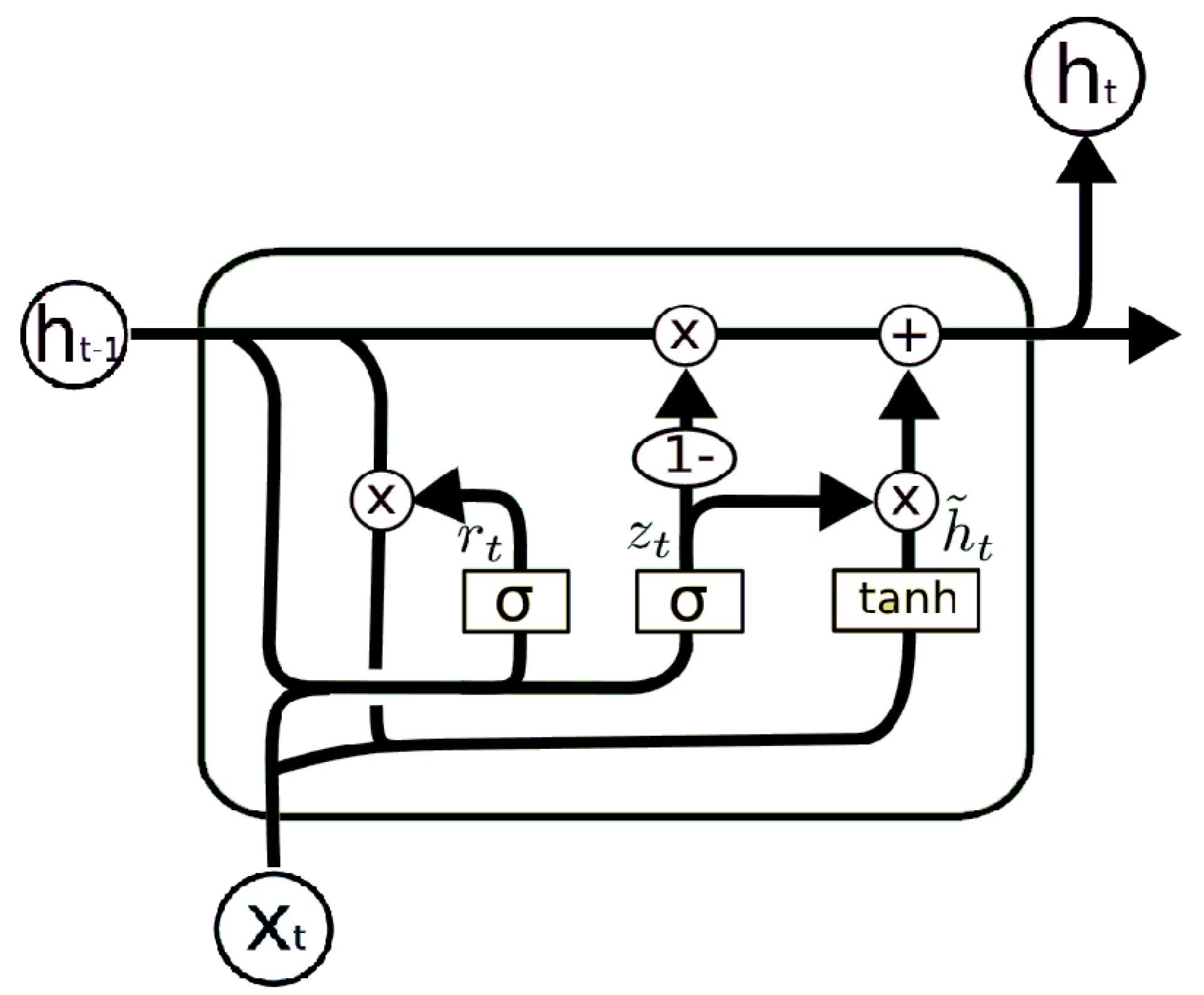
Gated recurrent units (GRU) were first proposed by [49] as a simplified and efficient modification of traditional RNN and LSTM cells. GRU models have successfully been applied to sequence modelling problems in the past [50,51], which makes them good candidates as a benchmark model for our paper. Unlike LSTM, GRU only has two gates, the update gate and the reset gate; since there is no output gate, GRU has no control over the memory content of the unit. Due to simple gating units and less modulation of the flow of information inside the unit, GRU has less training parameters than LSTM. Furthermore, the lack of a forget gate gives GRU the ability to keep information from distant past steps, without discarding it through time or forgetting information that is irrelevant to the prediction. A simple GRU block is presented in Figure 2 below.

An update gate $z_t$, for timestep t, helps the model determine the amount of previous information that needs to be passed to the next unit. The advantage of the update gate is that it copies all the past information and eliminates the vanishing gradient problem. The reset gate, $r_t$, is a replacement of the forget gate from LSTM that determines the amount of information to forget/reset. The equations of GRU can be written as follows.

$$z_t=\sigma \left(W_z·\left[h_{t-1},x_t\right]+b_z\right)$$

(10)

$$r_t=\sigma \left(W_r·\left[h_{t-1},x_t\right]+b_r\right)$$

(11)

$${\tilde{h}}_t=tanh\left(W_h·\left[r_t\odot h_{t-1},x_t\right]+b_h\right)$$

(12)

$$h_t=\left(1-z_t\right)\odot h_{t-1}+z_t\odot {\tilde{h}}_t$$

(13)

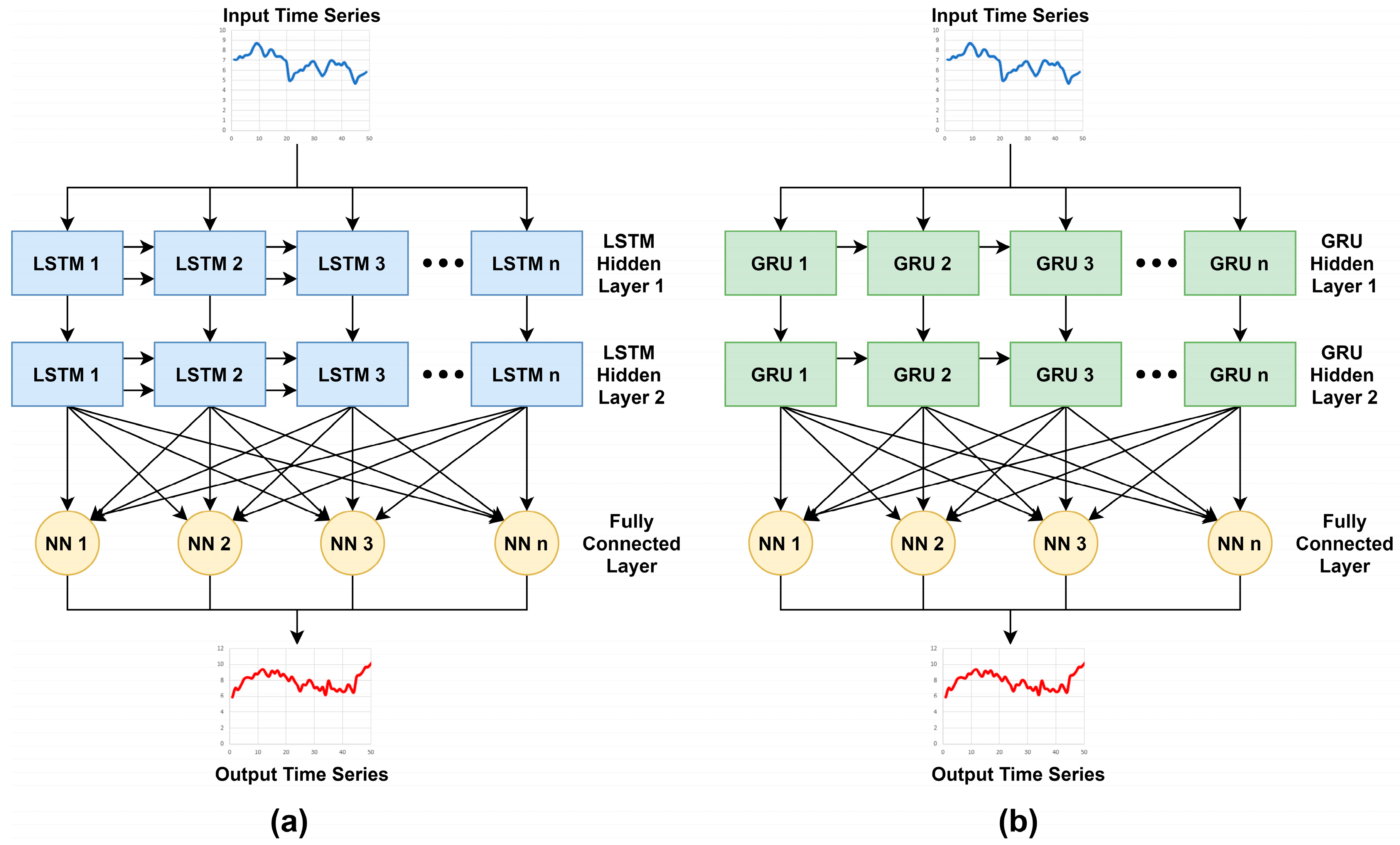
In Figure 3, the LSTM and the GRU models are illustrated, which are used as the benchmark models for our proposed model. The LSTM model is comprised of two hidden layers of the LSTM chain of 50 LSTM cells each (the number of cells corresponds to the number of input timesteps; please refer to Section 2.5 for more information). Finally, an FC layer consisting 50 neurons with linear activation was used as the output layer. Similarly, we also used a GRU model with two hidden layers of the GRU chain with 50 units each followed by an FC layer of 50 with linear activation. The number of hidden layers for the LSTM layer was determined using the Tabu search method; please refer to [52] for more details about the architecture search using the mentioned method. The complete parameter information of LSTM and GRU models is listed in

Table 1. LSTM model hyperparameters.

Layer Name	Activations	Kernel Initial Distribution	Number of Neurons/Cells	Number of Trainable Parameters
LSTM	Sigmoid + Tanh	Normal	50	20,200
LSTM	Sigmoid + Tanh	Normal	50	20,200
FC	Linear	Normal	50	2550
Total			150	42,950

and

Table 2. GRU model hyperparameters.

Layer Name	Activations	Kernel Initial Distribution	Number of Neurons/Units	Number of Trainable Parameters
LSTM	Sigmoid + Tanh	Normal	50	15,300
LSTM	Sigmoid + Tanh	Normal	50	15,300
FC	Linear	Normal	50	2550
Total			150	33,150

, respectively.

2.2. Convolutional Neural Networks

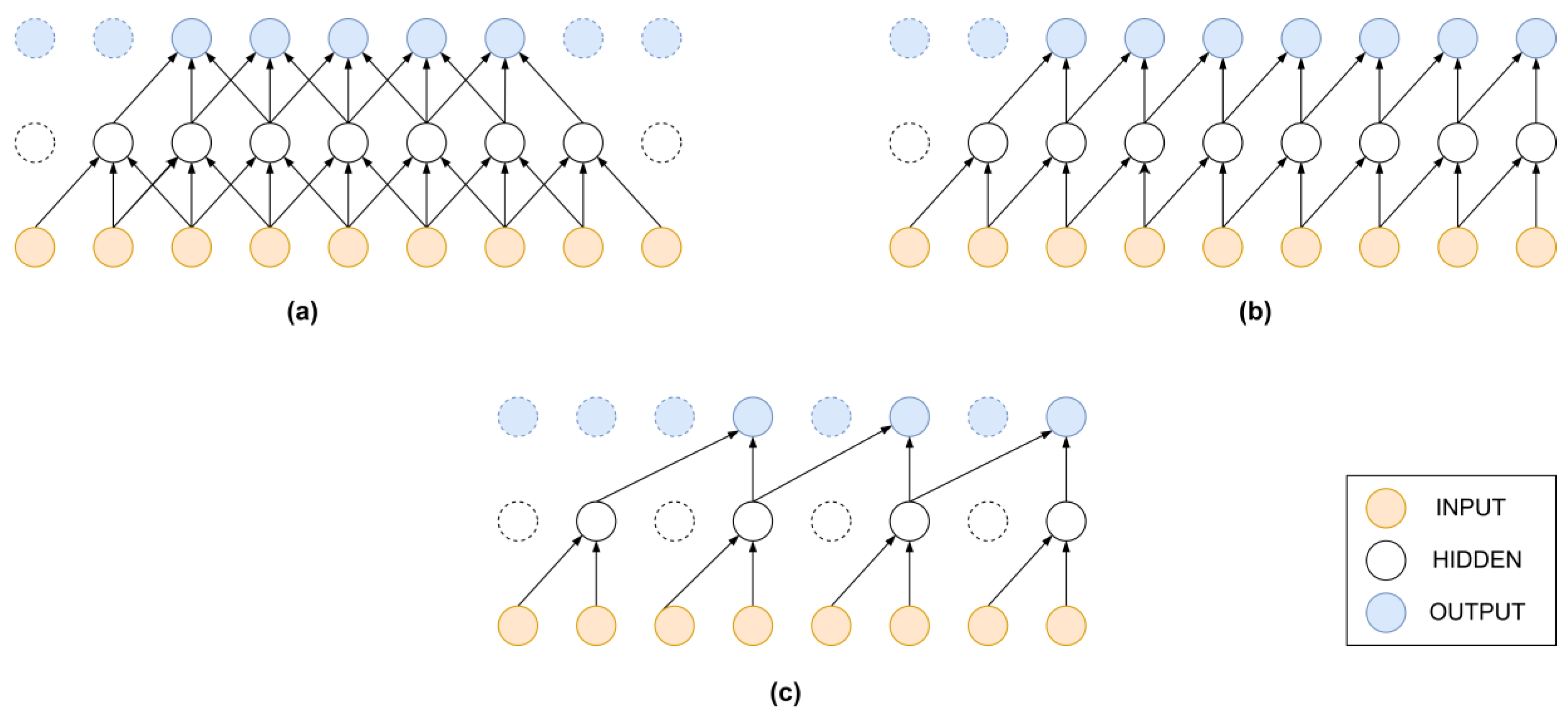
Convolutional neural networks (CNN) are known for their outstanding performance on image (2D data) related machine learning tasks, such as image segmentation, object recognition, and super resolution. A modified version of CNN, known as 1D CNN [30,53], has been developed for time series and other 1D data (sound, vibration, sentences, etc.). CNN layers as shown in Figure 4a are comprised of filters that capture the local correlation of nearby data points, instead of the conventional full connection. The filters are made up of convolutional kernels that share the same weights. Each 1D CNN layer can be mathematically represented as follows:

$$y_{ij}^k=f\left({\left({\omega }^k\ast x\right)}_{ij}+b_k\right)$$

(14)

where $\ast$ is the convolution operation, y is the output, x is the input, ${\omega }^k$ is the weight matrix, and $b_k$ is the bias matrix of the k^th layer. In Equation (14), i and j are the number of filters and neurons, respectively. In the above equation, f is the activation function. The rectified linear unit (ReLU) is one of the widely utilized activation functions for CNN layers. A modified version of ReLU known as scaled exponential linear unit (SELU) was proposed by [54], which induces self-normalization properties on CNN layers. Furthermore, SELU avoids the vanishing gradient problem while normalizing the network and speeding up the training process. The equations for ReLU and SELU are as follows,

$$\mathrm{ReLU}\left(z\right)=\max \left(0, z\right)$$

(15)

$$\mathrm{SELU}\left(z\right)=\lambda ·\max \left(\alpha e^z-\alpha , z\right)$$

(16)

The authors of [54] calculated the values for $\lambda$ and $\alpha$ as 1.05070098 and 1.67326324, respectively.

Causal convolution [55] is a restrictive variation of CNN, in which the timestep order must not be violated. In causal CNN, the output at any timestep t only uses the information from previous steps. Figure 4b illustrates the flow of information in a causal CNN structure. Because of this time dependency characteristic, causal CNN are used for time series classification and prediction tasks. Mathematically, we can represent a layer of causal CNN as follows,

$$y_{ij}^k=f\left({\left({\omega }_j^k\ast x^{k-1}\right)}_i+b_k\right)$$

(17)

where $\ast$ is the convolution operation, y is the output, $x^{k-1}$ is the input to the layer, ${\omega }^k$ is the weight matrix, and $b_k$ is the bias matrix of the k^th layer. In Equation (17), i and j are the number of filters and neurons, respectively. Unlike standard convolution, causal convolution guarantees that only instantaneous data are used, and future features are excluded during the training process. Thus, the final prediction of the causal architecture p(x_t+1|x₁, x₂, …, x_t) is independent of x_t+1, x_t+2, …, x_T. Causal convolution models make predictions in a sequential manner, and predictions of a layer are fed back into the next layer to predict the next sequence. Unlike RNN, causal convolution models do not have recurrent connections, and all the conditional predictions can be made in parallel, hence being faster to train than RNNs.

A dilated causal convolution also known as à trous convolution is a variant of CNN, where the filter is applied to a larger area than its kernel length by skipping inputs at certain steps. This technique was introduced by [56] to expand the size of CNN’s receptive field of images without modifying the data structure. The same technique can be applied to the time series data [57,58] to expand the data length effectively without increasing the neural network structure, as shown in Figure 4c. Due to its sparse connection and weight sharing mechanism, dilated convolution networks can automatically learn translationally-invariant features from longer input time series while having fewer trainable parameters than conventional CNN.

2.3. Residual Dilated Convolutional Neural Network

Residual convolutional neural networks were first proposed by [59] to tackle the problem of training deep learning models. Intuitively, by adding more layers, a CNN architecture should learn more complex functions and improve the prediction accuracy. However, the authors in [59] noted in their paper that deeper CNN models are not necessarily better at learning features. During the training of deeper models, a degradation problem was uncovered. The paper reported that such degradation was not due to overfitting, because adding more layers to the network counterintuitively increased the training error. With the increasing depth of the CNN model, the accuracy of the model becomes saturated and then starts degrading. This identifies the underlying problem of how the gradient descent-based optimization algorithm works. The authors proposed a shortcut connection by skipping a few layers of convolution and copying an identity matrix to the input of the following layer. The shortcut identity connections were designed in a way that all the information from the previous layer was always passed through to the next connected layer. In the residual learning method, for the mapping function (output) of a few stacked convolution layers $H\left(x\right)$, the shortcut connections force the network to learn residual function $H\left(x\right)-x$ instead. Thus, the underlying mapping function for stacked layers with an identity shortcut, also known as the residual block, becomes $f\left(x\right)=H\left(x\right)-x$. Therefore, for a residual block, the mathematical formulation can be written as follows,

$$y=f\left(\omega \ast x\right)+x$$

(18)

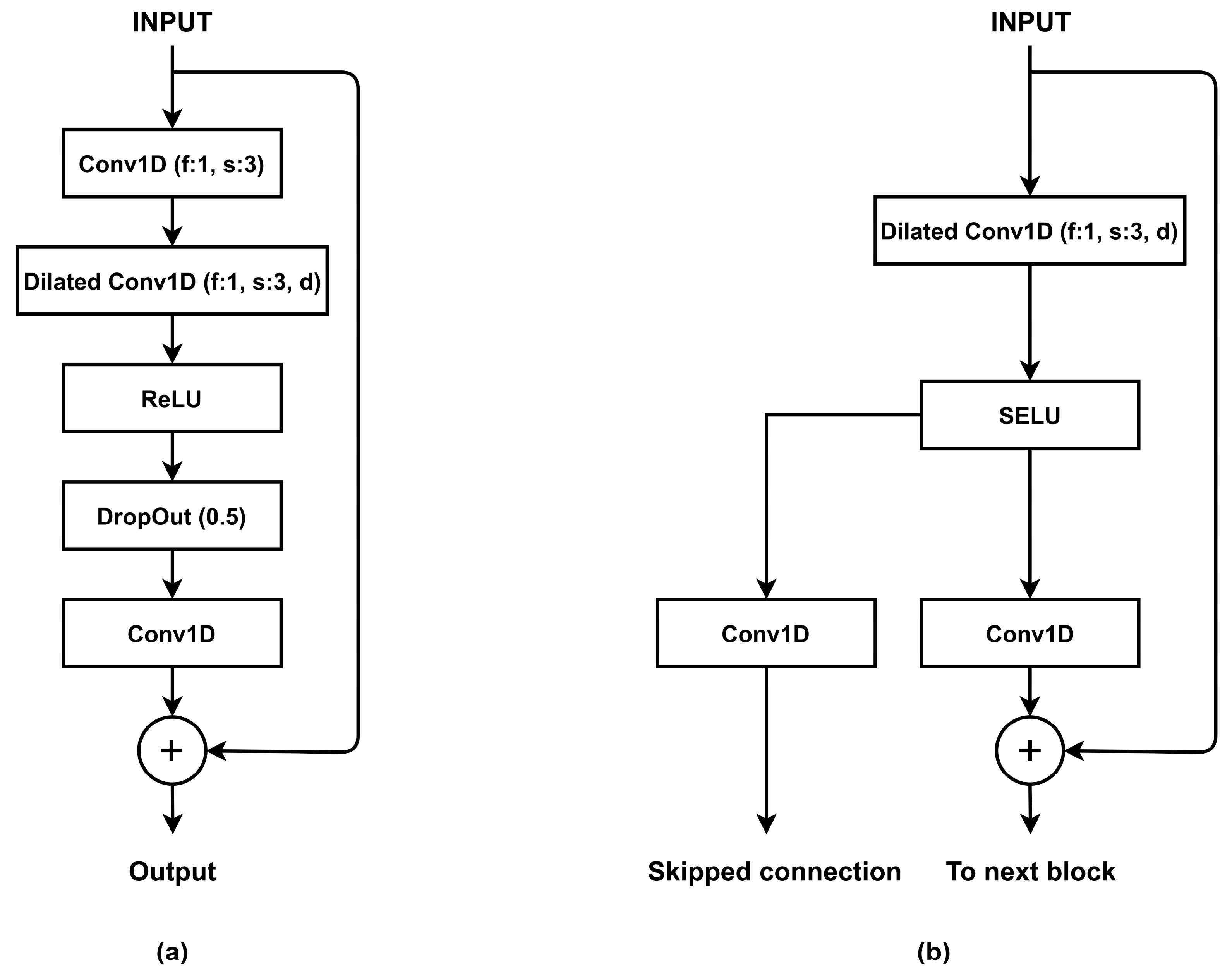
where x and y are the input and output of the residual block. According to the above function, the dimensions of x and $f\left(\omega \ast x\right)$ must be the same, else a linear projection can be applied to match the dimensions. The above modification to the traditional CNN architecture for image data was also experimented on time series data by replacing the 2D convolution layers with 1D convolution layers. WaveNet was proposed by [35] to generate raw audio waveforms. The WaveNet architecture consists of conditional residual blocks and skipped connections. Dilated convolution layers are used instead of standard convolution layers to expand the receptive field of networks. Several variations for the residual blocks for time series data have been proposed for different time series tasks. The work in [34] proposed a CNN-LSTM hybrid network with dilated convolution residual blocks (Figure 5a). The residual block proposed for the CNN-LSTM model is comprised of a dilated convolution layer followed by a ReLU activation and a dropout layer for better generalization. Another variation with skipped connection and the self-normalizing SELU activation function was proposed by [60]. The author proposed the residual block (Figure 5b), and ReLU activation was replaced by SELU activation to remove bias from the network and also improve generalization due to SELU’s self-normalization properties [54]. As noted by the author, unlike other time series prediction models, this architecture does not require data preprocessing to improve performance.

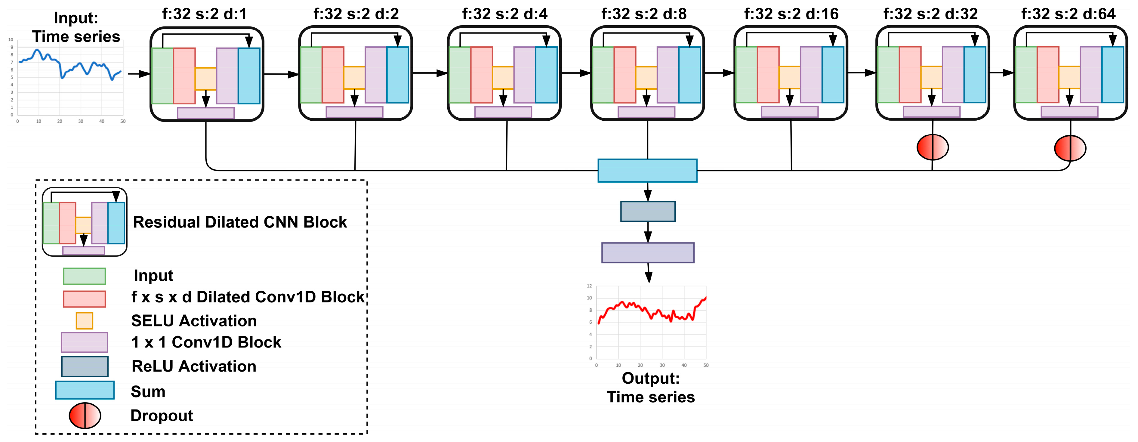
We used a generative time series forecasting model SeriesNet proposed by [60] as one of our benchmark models, a variant of residual-DCCNN. We also tested the CNN-LSTM hybrid model during our experiments, but the model was not able to converge using our sliding window training method (refer to Section 4), therefore being excluded from our benchmark list. The complete architecture of the SeriesNet is shown in Figure 6, and residual blocks and the complete architecture’s hyperparameters are listed in

Table 3. Residual block hyperparameters.

Layer ID	Layer Name	Connection	Activations	Kernel Initial Distribution	Parameters (Filter, Kernel Size, Dilation)	Number of Trainable Parameters
1	Dilated Conv1D	Input	SELU	Truncated Normal	(32, 3, d)	64
a	Conv1D	1	Linear	Truncated Normal	(1, 1, NA)	32
b	Conv1D	1	Linear	Truncated Normal	(1, 1, NA)	32
Total						128

and

Table 4. SeriesNet hyperparameters.

Layer ID	Layer Name	Connection (to Layer ID)	Parameters (Dilation)	Number of Trainable Parameters
1	Residual Block	Input	1	128
2	Residual Block	1a	2	128
3	Residual Block	2a	4	128
4	Residual Block	3a	8	128
5	Residual Block	4a	16	128
6	Residual Block	5a	32	128
7	Residual Block	6a	64	96
8	Dropout	6b	NA	0
9	Dropout	7b	NA	0
10	Sum	1b, 2b, 3b, 4b, 5b, 8, 9	NA	0
11	ReLU	10	NA	0
12	Conv1D (1 × 1, Linear)	11	NA	1
Total				865

, respectively. As illustrated in Figure 6, the final predictions of SeriesNet were made using parameterized skipped connections of the residual block. As noted by the author, the model uses skipped connection instead of only using the final output of residual blocks to ensure that the latent representation of dilated convolution layers is not overly influenced by past trends that may not be relevant to the present prediction. The L2-norm was applied to every convolution layer to further improve the generalization, and a truncated normal distribution was used for kernel initialization of each layer for faster convergence. In this architecture, dilated convolution layers have a fixed number of filters (i.e., f: 32) with a constant kernel size of three (s:3), but an increasing number of dilations (d) in the order of 1, 2, 4, 8, 16, 32, and 64 for 7 residual blocks. Furthermore, an 80% dropout rate was added for the last two residual blocks’ skipped connections. As listed in Table 3, the residual block had two output layers, residual connection a, and skipped connection b. In Table 4, the connection column corresponds to the layer id, and a and b are the residual and skipped connections of the residual blocks. Layer id 7 had only 96 trainable parameters as the residual connection of the seventh residual connection was not used during training. The element-wise sum of the skipped connection of each residual block was followed by a ReLU activation. The output layer was a 1 × 1 convolution layer with linear activation. Thus, the length of the input and output data was the same and forecasts were made in a direct manner.

2.4. Residual U-Net Architecture

The U-net architecture was proposed by [61] for biomedical image segmentation. The key feature of this architecture is the ability to use low-level features while retaining high-level semantic information. The idea behind U-net is similar to residual networks. In U-net, the low-level features are copied to corresponding high-level features to create a path for information to propagate between low- and high-level convolution layers. This method allows backpropagation of errors between layers and makes training deep learning models easier. Using the idea from U-net and residual networks, some researchers have proposed a hybrid model by replacing the plain convolution layers of U-net with residual blocks. The work in [62] proposed a deep residual U-net architecture (ResUnet) for extracting road from aerial images. In the ResUnet architecture, residual blocks are used to ease training, and the skipped long connection facilitates the flow of information between low levels and high levels without degradation. ResUnet architectures are also robust to the noise present in training data, as shown by [36], where ResUnet outperformed the residual networks. In [37], the authors showed some experiments with the ResUnet architecture and residual block structure to improve semantic segmentation of satellite images. In time series data applications, U-net architectures are applied to model traffic information [63]. Spatio-temporal U-net (ST-UNet) was proposed for modeling graph-structured time series. By using dilated recurrent skip connections, the ST-UNet architecture can extract multi-resolution temporal dependencies.

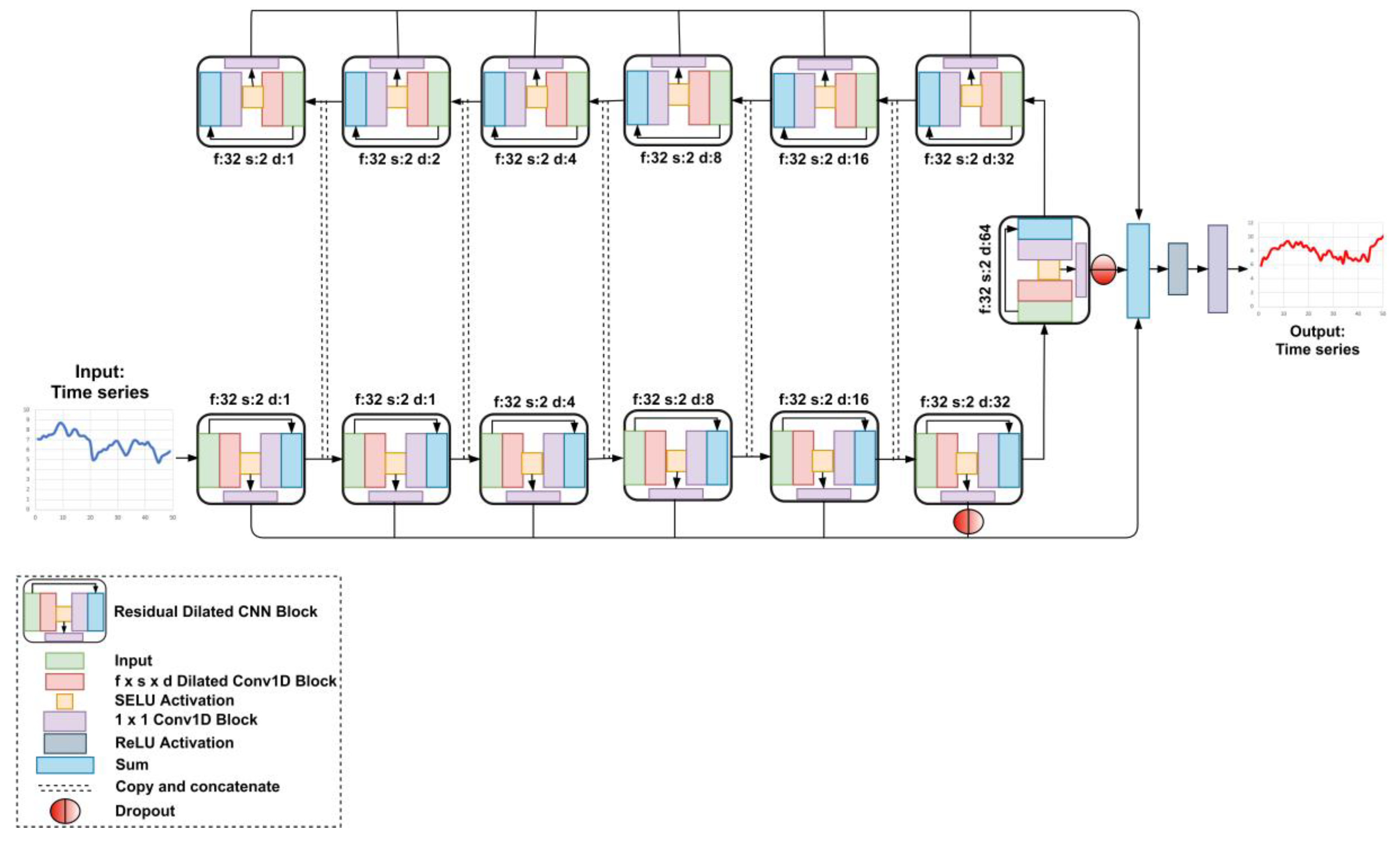
In this paper, we investigated a ResUnet architecture, consisting of the residual blocks from SeriesNet. As shown in Figure 7, we used the bottom 6 residual blocks similar to SeriesNet, then used the 7th block (the one with the highest dilation rate) as a bridge to transfer information to the upper 6 residual blocks. This architecture resembled an encoder-decoder network [64] with increasing numbers of dilation units; the highest dilation reached a value of 64 steps, then a decreasing number of dilations was applied to residual blocks. The number of residual blocks before and after the bridge was kept the same. Long skipped connections were applied to the corresponding top residual blocks from bottom residual blocks. The output of bottom blocks was copied and concatenated with the input of top blocks with the same number of dilations; thus, the temporal information due to dilation could be recovered or enhanced by top level residual blocks. Similar to SeriesNet, we used the sum of skipped connections of each residual block followed by ReLU activation to make the final prediction. Dropout was applied at the skipped connection of the sixth residual block to decrease the influence of past trends. Using the 1 × 1 convolution layer with linear activation at the output layer, the output steps were equal to the input steps, and the predictions were made in a direct manner. After some tests, we found a dropout rate of 80% to be suitable for the ResUnet architecture. The hyperparameters of ResUnet are listed in

Table 5. ResUnet hyperparameters.

Layer ID	Layer Name	Connection (to Layer ID)	Parameters (Dilation)	Number of Trainable Parameters
1	Residual Block	Input	1	128
2	Residual Block	1a	2	128
3	Residual Block	2a	4	128
4	Residual Block	3a	8	128
5	Residual Block	4a	16	128
6	Residual Block	5a	32	128
7	Residual Block	6a	64	128
8	Dropout	6b	NA	0
9	Dropout	7b	NA	0
10	Residual Block	7a	32	192
11	Residual Block	[10, 5a]	16	256
12	Residual Block	[11, 4a]	8	320
13	Residual Block	[12, 3a]	4	384
14	Residual Block	[13, 2a]	2	448
15	Residual Block	[14, 1a]	1	96
16	Sum	1b, 2b, 3b, 4b, 5b, 8, 9, 10b, 11b, 12b, 13b, 14b, 15b	NA	0
17	ReLU	16	NA	0
18	Conv1D (1 × 1, ReLU)	17	NA	1
Total				2593

. For the residual blocks’ hyperparameters, refer to Table 3.

2.5. The Proposed Model

The ResUnet structure allows the information to flow from the lower level residual blocks to the higher level ones. However, this alone is not enough to get a substantial gain in time series data. Since the residual blocks proposed in SeriesNet work best for univariate time series data, we noticed a major drawback in the ResUnet architecture. When merging the low-level features with high-level ones, the dimension of the data becomes modified, and our consistent univariate data flow as in SeriesNet becomes multivariate because of the concatenation of two one-dimensional outputs. We experimented by averaging, element-wise multiplication, and addition to overcome this drawback, but the results were poorer than ResUnet discussed in Section 2.4. Further, we focused our efforts on blocks for time series data.

The attention mechanism is typically used in RNN architectures to improve the model performance. The works in [65,66,67] are a few examples where attention blocks were proposed and used with LSTM architectures for time series forecasting. Attention blocks have also been used with CNN architectures [40,43,68,69] for image classification and time series data. One of the noteworthy contributions of the attention mechanism for time series forecasting can be found in [70]. We investigated this architecture for our application, but the results were not better than SeriesNet, so we skipped this in our benchmark list.

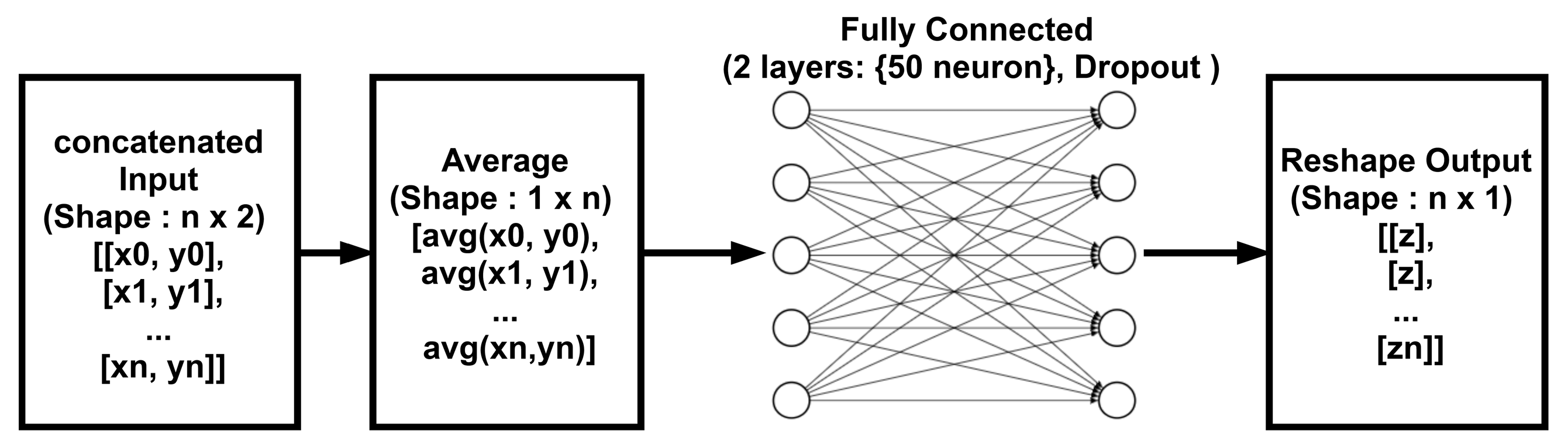
The proposed non-linear attention mechanism (Figure 8) consisted of two FC layers of equal length (50 neurons) with a dropout applied between them. The attention mechanism received a concatenated input X with two column vectors, then a row-wise average was calculated before feeding the data to a fully-connected layer. The row-wise average function was used to calculate the average mapping of residual blocks for each time series element without violating their timestep order, i.e., preserving temporal information. A dropout was applied to the output of the first FC layer before feeding into the next FC layer to prevent the saturation of FC layers during training. Finally, the output of the second FC layer was reshaped in order to comply with the CNN layers’ data input format. We applied sigmoid activation to the FC layers to ensure non-linearity in the FC layer output.

For the given input matrix $x_{ij}$ with i rows and j columns, we could represent our non-linear attention block as follows,

$$X_m={{\displaystyle \sum }}_{j=1}^n{x}_{ij}/n$$

(19)

$$h_1=\sigma \left({\omega }_1{X}_m+b_1\right)$$

(20)

$$h_2=\sigma \left({\omega }_2\left(h_1\odot \Xi \right)+b_2\right), with {\xi }_{mi}\sim p\left(\xi \right)$$

(21)

$$O=ve{c}_{1,n}^{n,1}\left(vec\left(h_2\right)\right)$$

(22)

where $X_m$ is the row-wise mean of input matrix $x_{ij}$ and n is the number of elements in the row of the matrix. $h_1$ and $h_2$ are the outputs of the first and second FC layer. In Equation (21), $(h_1\odot \Xi )$ represents the dropout applied to the input of the second FC layer, where $\odot$ is the element-wise (Hadamard) product, ${\xi }_{mi}$ is the elements of the mask matrix $\Xi$, and $p\left(\xi \right)$ represents the Bernoulli dropout, $Bernoulli\left(1-p\right)$, with dropout probability $p$. $O$ is the output of the attention block, where the output vector of the second FC layer is reshaped from 1 × n to n × 1 to conform with the standard input format of the 1D convolution layer. The dropout rate applied to the output of the first FC layers in this mechanism was kept at 50%.

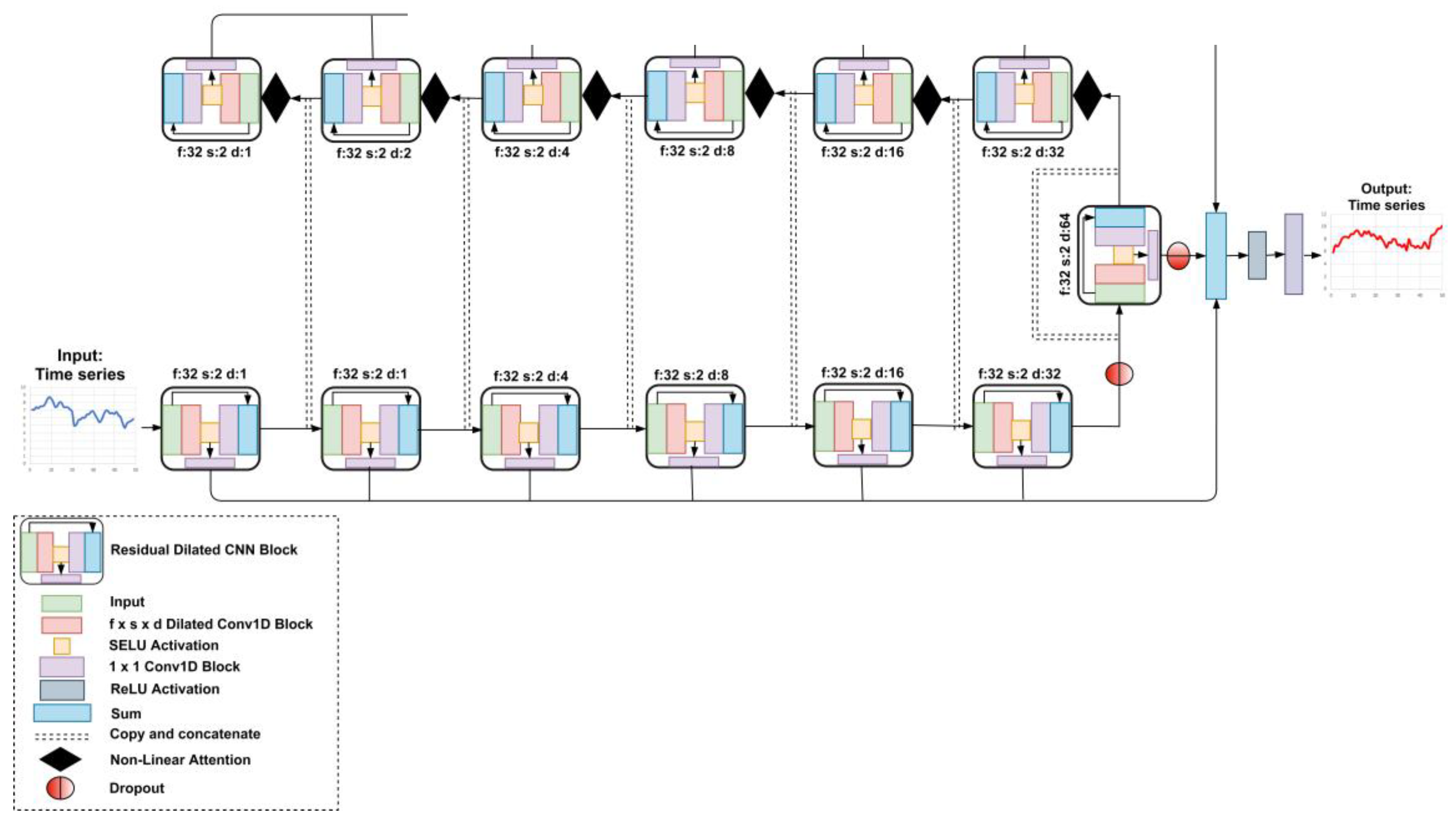
We used the proposed nonlinear attention blocks in ResUnet discussed in Section 2.4 with minor modifications as shown in Figure 9. We applied the attention blocks to the input of higher level residual blocks, transforming the concatenated vectors to a single output vector by applying the row-wise average and finding the nonlinear relationship between each timestep element using FC layers with sigmoid activation. The residual attention U-net (ResAUnet) architecture’s skipped connections were similar to those of ResUnet with the exception being that the attention block was also used to bypass the information by skipping the bridge connection of the residual block with the highest dilation value. In our proposed architecture, the feature mapping of lower level residual blocks was combined with the feature mapping of higher level one and then fed into the residual block with the same dilation value as the corresponding lower level residual block. In order to limit the over influence of past trends in the training of higher level residual blocks, we applied a dropout of 80% before the bridge connection and also at the skipped output of the 7th residual block. Combined with nonlinear attention, this mechanism of information flow allowed the architecture to learn complex relationship between the causal outputs of different dilation levels. Similar to SeriesNet, the number of output timesteps was equal to the input (i.e., 50 timesteps). The hyperparameters of the proposed attention block and ResAUnet are listed in

Table 6. Nonlinear attention block hyperparameters.

Layer ID	Layer Name	Connection	Activations	Kernel Initial Distribution	Parameters (No. of Neurons)	Number of Trainable Parameters
1	Row-wise average	Input	NA	NA	NA	0
2	FC layer	1	Sigmoid	Normal	50	2550
3	Dropout	2	NA	NA	NA	0
4	FC layer	3	Sigmoid	Normal	50	2550
5	Reshape (n, 1)	4	NA	NA	NA	0
Total						5100

and

Table 7. Residual attention U-net (ResAUnet) hyperparameters.

Layer ID	Layer Name	Connection (to Layer ID)	Parameters (Dilation)	Number of Trainable Parameters
1	Residual Block	Input	1	128
2	Residual Block	1a	2	128
3	Residual Block	2a	4	128
4	Residual Block	3a	8	128
5	Residual Block	4a	16	128
6	Residual Block	5a	32	128
7	Dropout	6a	NA	0
8	Residual Block	7	64	128
9	Dropout	8b	NA	0
10	Attention	[7,8a]	NA	5100
11	Residual Block	10	32	128
12	Attention	[11a,5a]	NA	5100
13	Residual Block	12	16	128
14	Attention	[13a,4a]	NA	5100
15	Residual Block	14	8	128
16	Attention	[15a,3a]	NA	5100
17	Residual Block	16	4	128
18	Attention	[17a,2a]	NA	5100
19	Residual Block	18	2	128
20	Attention	[19a,1a]	NA	5100
21	Residual Block	20	1	96
22	Sum	1b, 2b, 3b, 4b, 5b, 6b, 9, 11b, 13b, 15b, 17b, 19b, 21b	NA	0
23	RELU	22	NA	0
24	Conv1D (1 × 1, Linear)	23	NA	1
Total				32,233

, respectively.

2.6. Wind Speed Data

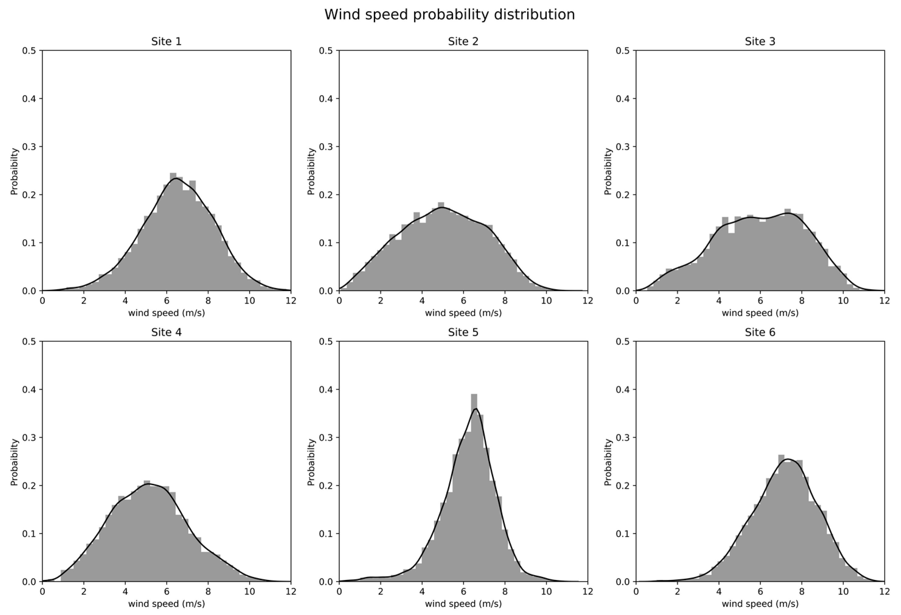
For the comparison of the models presented in Section 2, we used an open access dataset publish by [71] under a creative commons license at https://0-www-sciencedirect-com.brum.beds.ac.uk/science/article/pii/S2352340919306456. The published dataset presents the wind speed, wind direction, and wind power data of 12 different sites in the state of Tamil Nadu in India. The measurements were recorded using anemometers and wind vanes at a height of 100 m at a regular interval of 10 min throughout the year. The dataset consists of the measurements for the years 2014, 2015, and 2016 for all 12 locations. To compare the model’s performance, we chose first six locations and 6050 wind speed timesteps from the datasets, which corresponded to the timeline of January to mid-February of 2014. The statistical features and collection site details of the dataset used in this paper are listed in

Table 8. Wind sites’ location and wind speed statistical features.

Wind Site	Location		Wind Speed (m/s)
	Latitude	Longitude	Maximum	Minimum	Mean	Standard Deviation
1	08°51′39.30″ N	77°53′11.40″ E	11.77	0.53	6.53	1.73
2	10°34′33.20″ N	77°41′21.30″ E	10.63	0.07	4.99	2.06
3	10°44′36.70″ N	78°08′17.00″ E	11.38	0.53	5.95	2.16
4	08°57′44.05″ N	77°43′12.73″ E	11.36	0.27	5.15	1.88
5	10°03′21.90″ N	78°42′46.00″ E	10.82	0.11	6.23	1.33
6	09°04′47.50″ N	78°17′44.30″ E	11.56	0.99	7.16	1.58

below followed by the probability density plot calculated using kernel density estimation [72], presented in Figure 10.

2.7. Training Method

In general, the performance of an ANN model is measured using the k-fold validation method. This method is effective in determining the model’s performance when the data used for training are not time-dependent, e.g., image data, non-time series regression, etc. Another method used for testing the time series prediction model is the training and testing split, where data are split for training and testing the model. This method requires a large historical dataset that can be used to train the complex models at the training time. The model is then used predict on the testing data split to validate the model accuracy. Many researches referred to in Section 1 used this method for wind speed prediction evaluation. However, in real-world applications where historical data for a distant past horizon are not available, the training and testing split method cannot be applied successfully. Furthermore, the presence of stochastic trends in time series datasets makes it difficult to verify the performance of such model for distant future timesteps. Another method of training the time series prediction model is known as expanding window validation. In the expanding window validation method [73,74], the model is retrained every time new data are available. This method is popular for validating prediction models for financial and economic time series data. We investigated this method, but the increasing amount of data in the training pool made the training period longer, and the model took more time to converge.

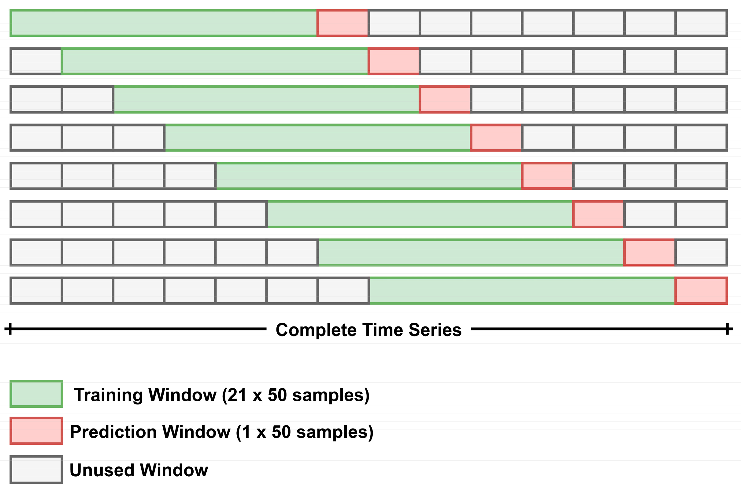
In our research, we used the sliding window technique [75,76,77,78], also known as the rolling window, moving window, or walk-forward technique. The sliding window technique is more robust to the stochastic changes in the data trend and can be applied to smaller datasets as the window size is smaller. As shown in Figure 11, we used a training window of 21 sets of 50 wind speed timesteps to train our model and then predicted the next 50 timesteps using the last set of data in the training window. For every new prediction window, the training window used a new set of 50 timesteps and discarded the oldest set of timesteps. The intuition behind this technique was that by discarding old data from the training window, we could limit the influence of distant past trends during model training and promote the learning of new trends in the data. This method also reduced the training time of the model as the number of training sets was always fixed. The training window size of 21 × 50 timesteps was chosen after testing the incrementing window size in multiples of 3, which was also the batch size used for training all models.

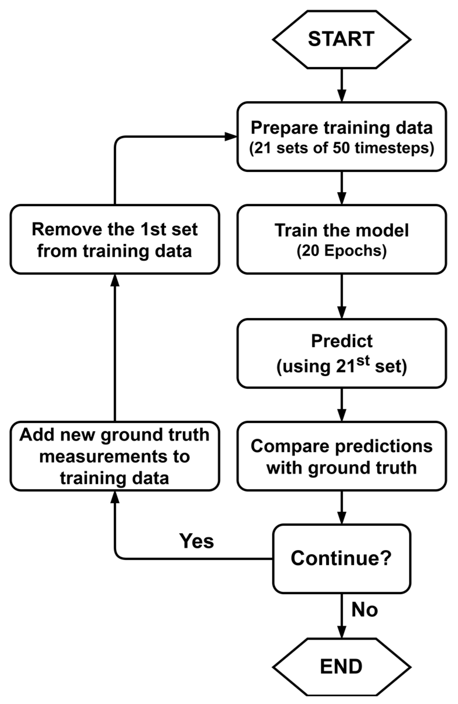
In order to facilitate a fair comparison of all benchmark models, we also used the results of simple the naive prediction model. The naive prediction model used in our benchmark model uses the current set of timesteps t to predict the next set t+1 as $Y_{t+1}=Y_t$. We used the stochastic optimizer Adam [48] to train and retrain all the models (LSTM, GRU, SeriesNet, ResUnet, and ResAUnet) with a learning rate of 0.0075, the exponential decay of the first moment equal to 0.9, the exponential decay of the second moment estimate equal to 0.999, and an epsilon value of ${10}^{-8}$. Models were trained for 50 epochs for each training window with a batch size of 3. The loss function used for training different models was the mean absolute error (MAE). For each wind speed site, the model’s weights were reinitialized to default weights in order to prevent the influence of trends from previous wind sites on the next site’s prediction. The training and prediction method used for the models in this study is shown as a flowchart in Figure 12.

3. Results

3.1. Performance Metrics for Forecast Accuracy

Usually, the performance of a regression model is judged using the root mean squared error (RMSE), mean absolute error (MAE), and mean absolute percentile error (MAPE). However, when it comes to the time series prediction model, MAE, RMSE, and MAPE were not sufficient to evaluate the model’s performance. RMSE depends on the scale of dependent variable and is sensitive to large deviation. MAPE is a scale independent measure. However, MAPE has the limitation of being infinite or undefined if there is a zero value in the series. Furthermore, MAPE can have an extremely skewed distribution in the case that the actual values are very close to zero. Therefore, we also used the “symmetric” MAPE (SMAPE) proposed in the Makridakis competition (M-3 competition) [79] for time series prediction models. We also investigated the mean squared log error (MSLE) for our performance evaluation. Since the MSLE measures the ratio between the actual value and the predicted value, large errors are not penalized if the both the actual and predicted values are large numbers. Furthermore, MSLE penalizes underestimates more than the overestimates. Another error metric we used is the normalized root mean squared error (NRMSE). NRMSE is the normalized version of RMSE, which facilitates the comparison between datasets and models with different scales. We also used the unscaled mean bounded relative absolute error (UMBRAE) [80] to compare the accuracy of different models using naive prediction results as the benchmark. UMBRAE is based on the mean bounded relative absolute error (MBRAE), but the final result is represented in terms of a ratio, rather than relative error. If UMBRAE is larger than one, the model has worse accuracy than the benchmark, and values smaller than one indicate better accuracy than the benchmark. UMBRAE is less sensitive to outliers and a is symmetric and scale-independent measure of model’s accuracy. The equations for calculating the performance/error metrics used in this paper are as follows.

$$\mathrm{MAE}=\frac{1}{n}{{\displaystyle \sum }}_{i=1}^n\left|x_i-{\tilde{x}}_i\right|$$

(23)

$$\mathrm{RMSE}=\sqrt[2]{\frac{1}{n}{{\displaystyle \sum }}_{i=1}^n{\left(x_i-{\tilde{x}}_i\right)}^2}$$

(24)

$$\mathrm{MSLE}=\frac{1}{n}{{\displaystyle \sum }}_{i=1}^n\log \left(\frac{x_i+1}{{\tilde{x}}_i+1}\right)$$

(25)

$$\mathrm{MAPE}=\frac{1}{n}{{\displaystyle \sum }}_{i=1}^n\left|\frac{{\tilde{x}}_i-x_i}{x_i}\right|$$

(26)

$$\mathrm{SMAPE}=\frac{2}{n}{{\displaystyle \sum }}_{i=1}^n\frac{\left|{\tilde{x}}_i-x_i\right|}{\left|x_i\right|+\left|{\tilde{x}}_i\right|}$$

(27)

$$\mathrm{NRMSE}=\frac{\sqrt[2]{\frac{1}{n}{{\displaystyle \sum }}_{i=1}^n{\left(x_i-{\tilde{x}}_i\right)}^2}}{x_{max}-x_{min}}$$

(28)

$$\mathrm{MBRAE}=\frac{1}{n}{{\displaystyle \sum }}_{i=1}^n\frac{\left|x_i-{\tilde{x}}_i\right|}{\left|x_i-{\tilde{x}}_i\right|+\left|x_i-{\tilde{x}}_i^{\ast }\right|}$$

(29)

$$\mathrm{UMBRAE}=\frac{\mathrm{MBRAE}}{1-\mathrm{MBRAE}}$$

(30)

where $x_i$ is the actual value, ${\tilde{x}}_i$ is the predicted value of the model, ${\tilde{x}}_i^{\ast }$ is the predicted value of the naive prediction method, and n is total number of predictions.

3.2. Comparison

We trained and tested the proposed model and benchmark models on six wind speed datasets. The models involved in this research were naive, LSTM, GRU, SeriesNet, ResUnet, and ResAUnet. No preprocessing was applied to the wind speed data in order to test the model’s performance on raw wind speed data. Each model’s input series length was 50, and a 50 step-ahead-prediction test was evaluated in this paper.

In

Table 9. Error metrics of different models on six site’s wind speed data. SMAPE, “symmetric” MAPE; UMBRAE, mean bounded relative absolute error.

Wind Data	Models	MAE (m/s)	RMSE (m/s)	MSLE (m/s)	MAPE (×100%)	SMAPE (×100%)	NRMSE (1)	UMBRAE (1)
Site 1	Naive	1.683	2.068	0.092	0.298	0.274	0.192	1.000
	GRU	1.359	1.694	0.063	0.259	0.218	0.157	0.843
	LSTM	1.356	1.688	0.063	0.262	0.220	0.157	0.853
	SeriesNet	1.304	1.618	0.058	0.248	0.211	0.15	0.804
	ResUnet	1.306	1.624	0.058	0.249	0.211	0.151	0.805
	ResAUnet	1.254	1.583	0.055	0.237	0.202	0.147	0.768
Site 2	Naive	2.631	3.171	0.328	0.767	0.529	0.306	1.000
	GRU	1.745	2.138	0.155	0.515	0.359	0.206	0.705
	LSTM	1.629	2.016	0.142	0.483	0.340	0.194	0.698
	SeriesNet	1.482	1.868	0.119	0.414	0.312	0.180	0.618
	ResUnet	1.504	1.879	0.125	0.423	0.323	0.181	0.632
	ResAUnet	1.353	1.707	0.107	0.389	0.296	0.165	0.584
Site 3	Naive	2.935	3.504	0.312	0.668	0.505	0.323	1.000
	GRU	1.839	2.235	0.136	0.456	0.322	0.206	0.657
	LSTM	1.773	2.151	0.129	0.443	0.312	0.198	0.679
	SeriesNet	1.527	1.916	0.104	0.375	0.278	0.177	0.575
	ResUnet	1.470	1.858	0.098	0.356	0.269	0.171	0.554
	ResAUnet	1.271	1.641	0.079	0.310	0.236	0.151	0.486
Site 4	Naive	1.710	2.194	0.158	0.438	0.357	0.198	1.000
	GRU	1.422	1.761	0.099	0.388	0.296	0.159	0.896
	LSTM	1.417	1.746	0.101	0.400	0.299	0.157	0.837
	SeriesNet	1.378	1.708	0.094	0.373	0.288	0.154	0.864
	ResUnet	1.390	1.717	0.095	0.375	0.290	0.155	0.873
	ResAUnet	1.288	1.624	0.085	0.350	0.268	0.146	0.810
Site 5	Naive	1.453	1.88	0.105	0.359	0.264	0.176	1.000
	GRU	1.073	1.402	0.061	0.287	0.193	0.131	0.779
	LSTM	1.081	1.408	0.062	0.290	0.195	0.131	0.803
	SeriesNet	1.059	1.374	0.060	0.282	0.192	0.128	0.773
	ResUnet	1.070	1.388	0.062	0.283	0.195	0.130	0.779
	ResAUnet	1.035	1.342	0.056	0.272	0.187	0.125	0.762
Site 6	Naive	1.731	2.138	0.085	0.28	0.257	0.204	1.000
	GRU	1.319	1.658	0.053	0.231	0.195	0.158	0.794
	LSTM	1.315	1.662	0.054	0.234	0.195	0.159	0.833
	SeriesNet	1.292	1.625	0.051	0.225	0.191	0.155	0.768
	ResUnet	1.295	1.630	0.052	0.226	0.192	0.156	0.771
	ResAUnet	1.295	1.617	0.050	0.223	0.192	0.154	0.781

, the prediction errors including MAE, RMSE, MSLE, MAPE, SMAPE, NRMSE, and UMBRAE of the six models are presented for different wind speed measurement sites. The comparison for the six sites is summarized below.

• LSTM and GRU models constantly performed better than the naive prediction model. Although the GRU model had a much lower number of parameters than LSTM, its performance was pretty close to LSTM. The LSTM model outperformed the GRU model on scaled error metrics like MAE, MSE, and MSLE on Site 1, Site 2, Site 3, and Site 4 data. However, we observed varying performance of LSTM and GRU for percentage-based metrics (MAPE and SMAPE) and scaled error metrics (NRMSE and UMBRAE). Overall, we saw the LSTM model performing slightly better than GRU.
• Compared to the LSTM and GRU models, we could clearly see a performance gain in SeriesNet. SeriesNet exhibited less error on all the metrics than the previous three models, with the only exception being UMBRAE on Site 4, where LSTM had less error by a scale of 0.027. This indicated that SeriesNet was able to learn the wind speed trends to predict 50-step-ahead data points much better than LSTM and GRU.
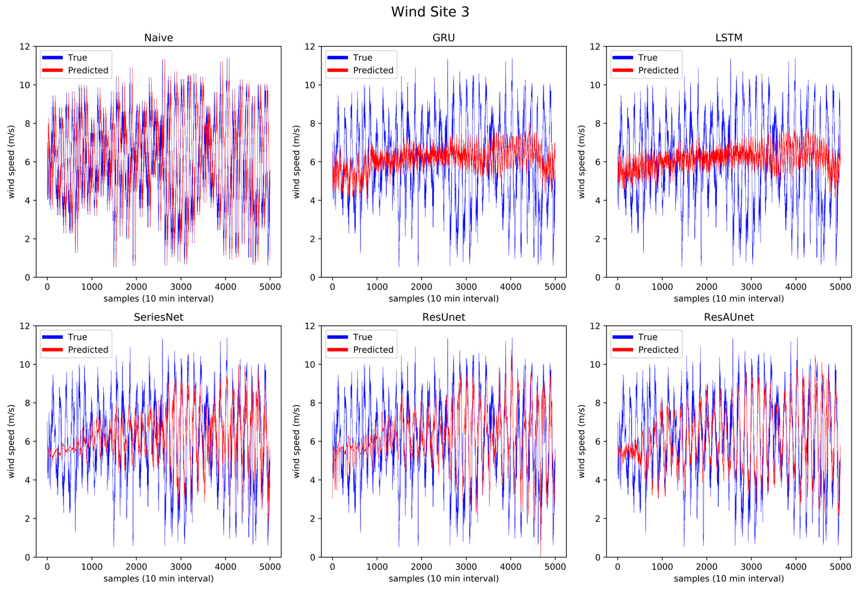
• The ResUnet model, which uses the residual blocks of SeriesNet, did not show any improvement for error metrics for all six data sites except for Site 3. The ResUnet model outperformed SeriesNet on all metrics for Site 3. Although the ResUnet model’s performance was not better than SeriesNet, it was either very close to or better than the LSTM model. Since the residual blocks of SeriesNet were designed for univariate time series data, degradation in the performance of ResUnet model was expected.

The proposed ResAUnet model with nonlinear attention blocks had the lowest error and best performance on all wind speed data sites with the only exception being Site 6, where SeriesNet showed better MAE, SMAPE, and UMBRAE. The ResAUnet model excelled on the RMSE, MSLE, MAPE, and NRMSE metrics for Site 6. By the evaluation of Table 8, we could conclude that nonlinear attention used in ResAUnet was helpful to improve the prediction accuracy for wind speed data.

3.3. Prediction and Error Plots

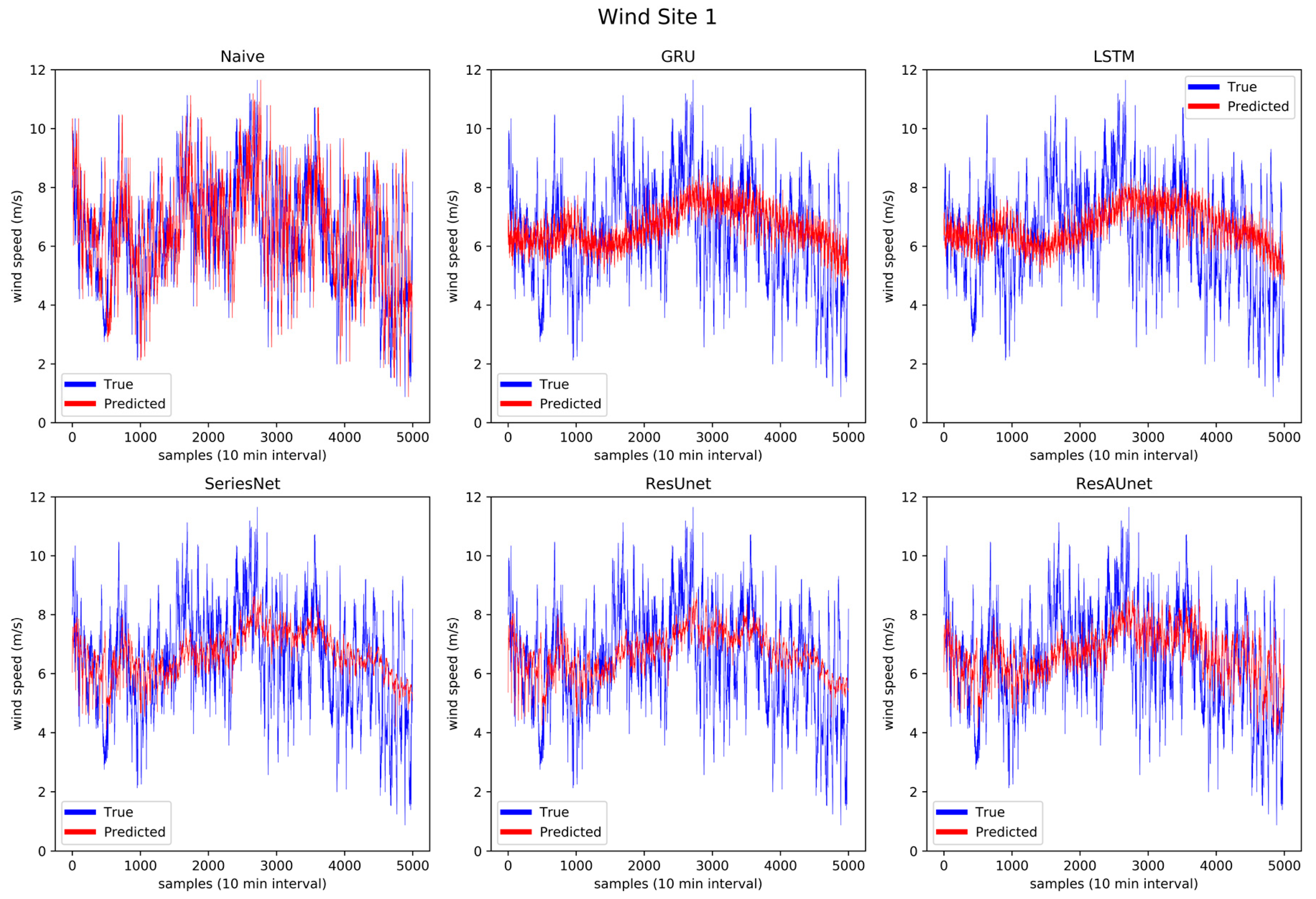
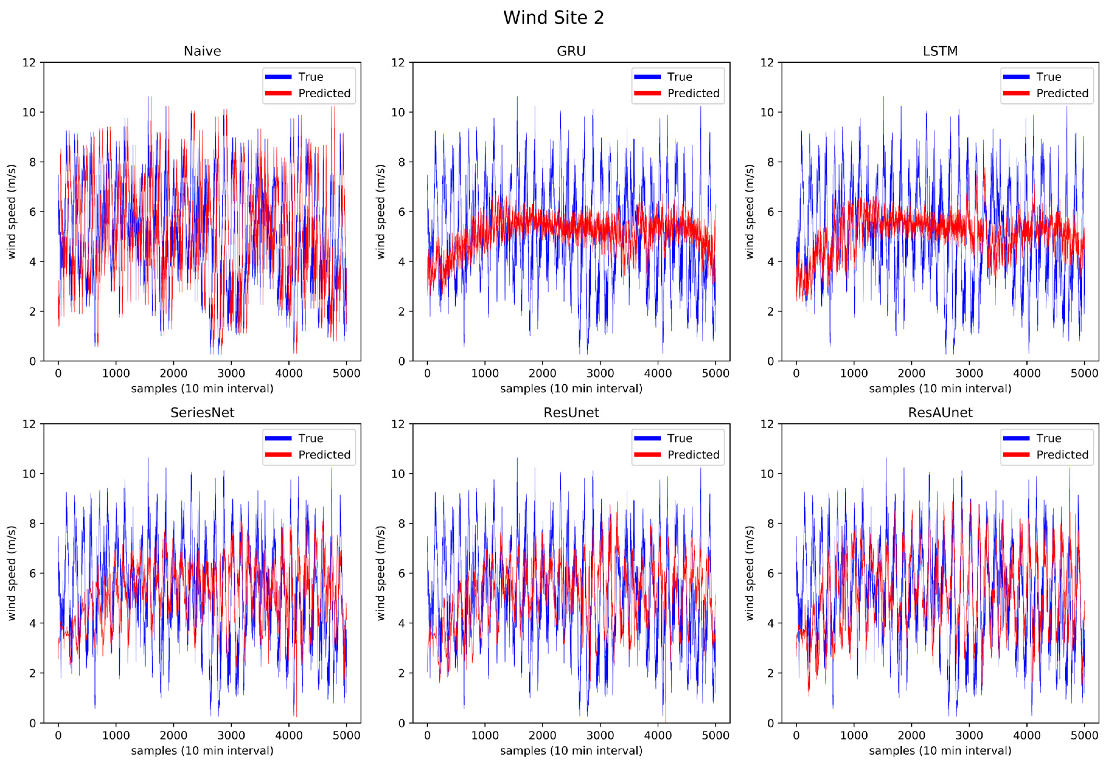
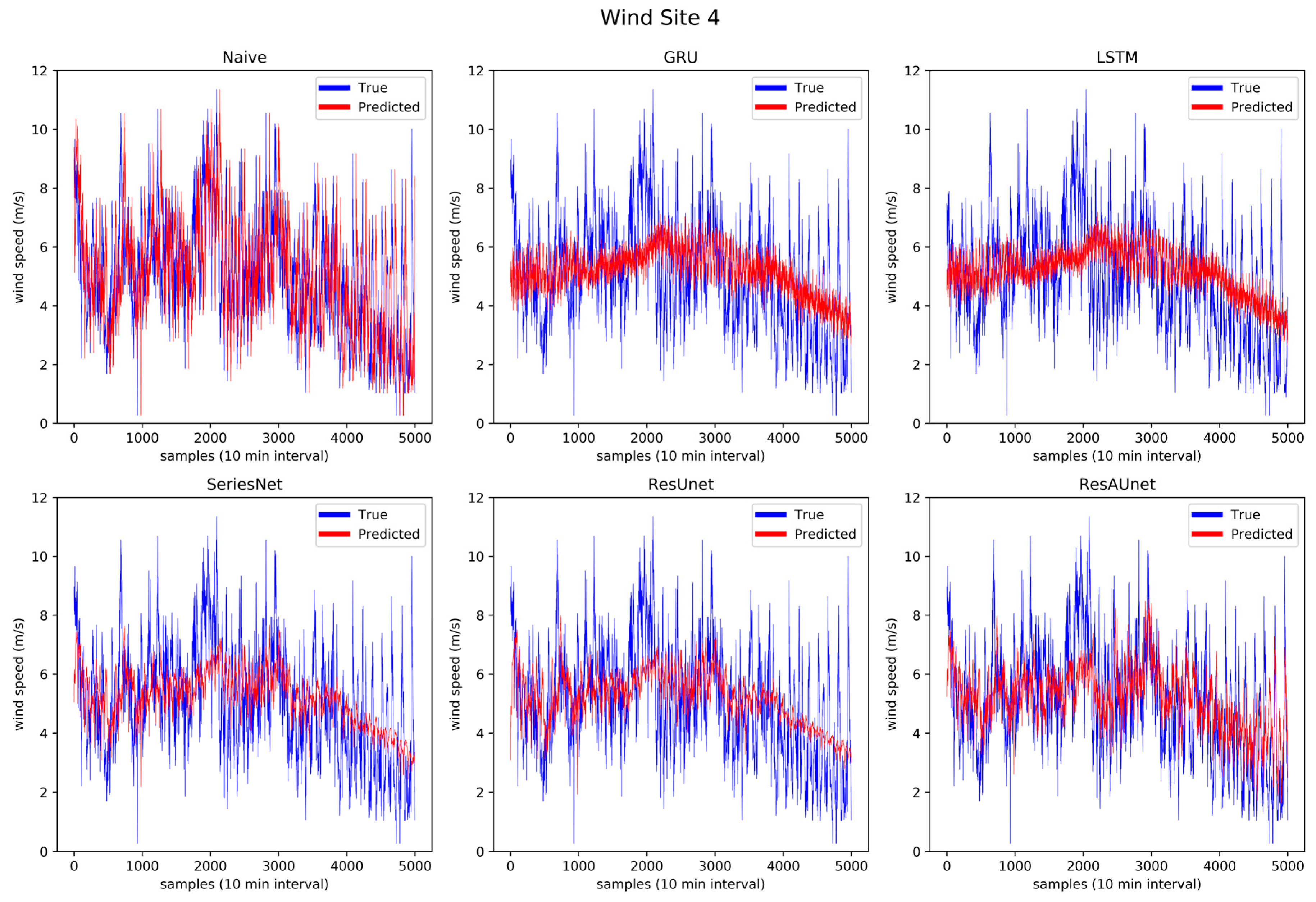
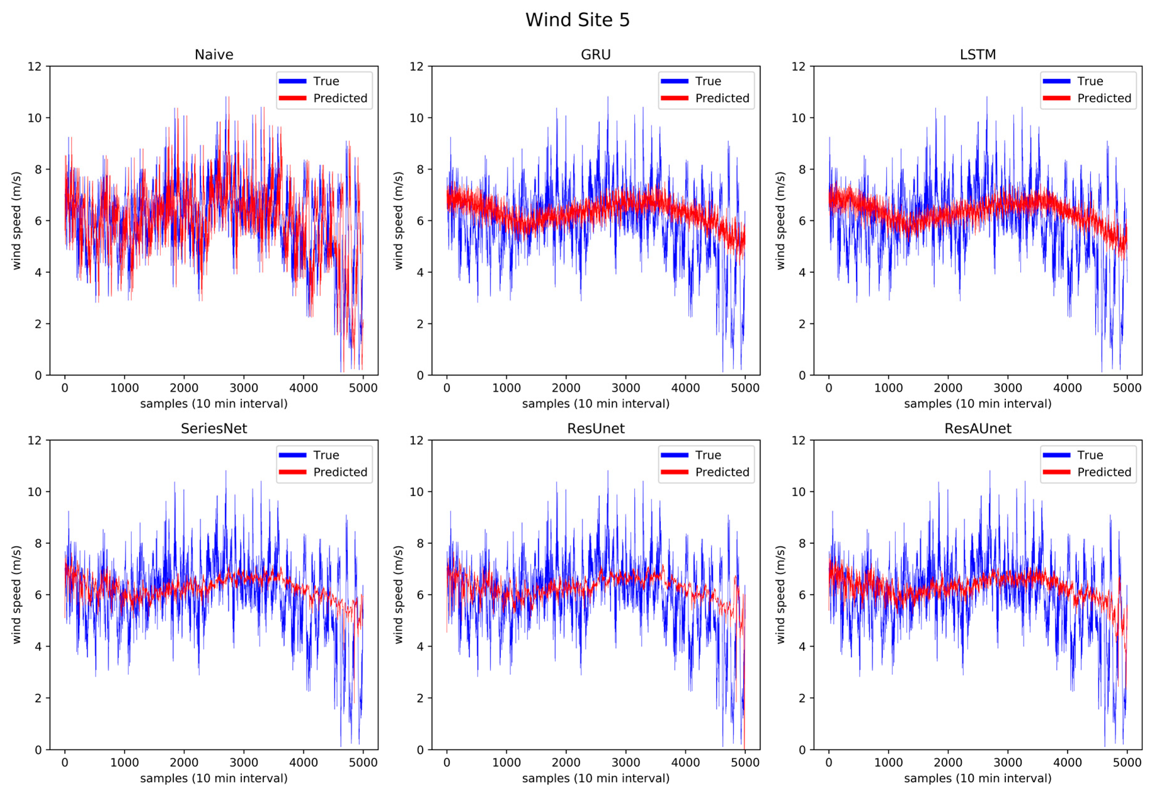
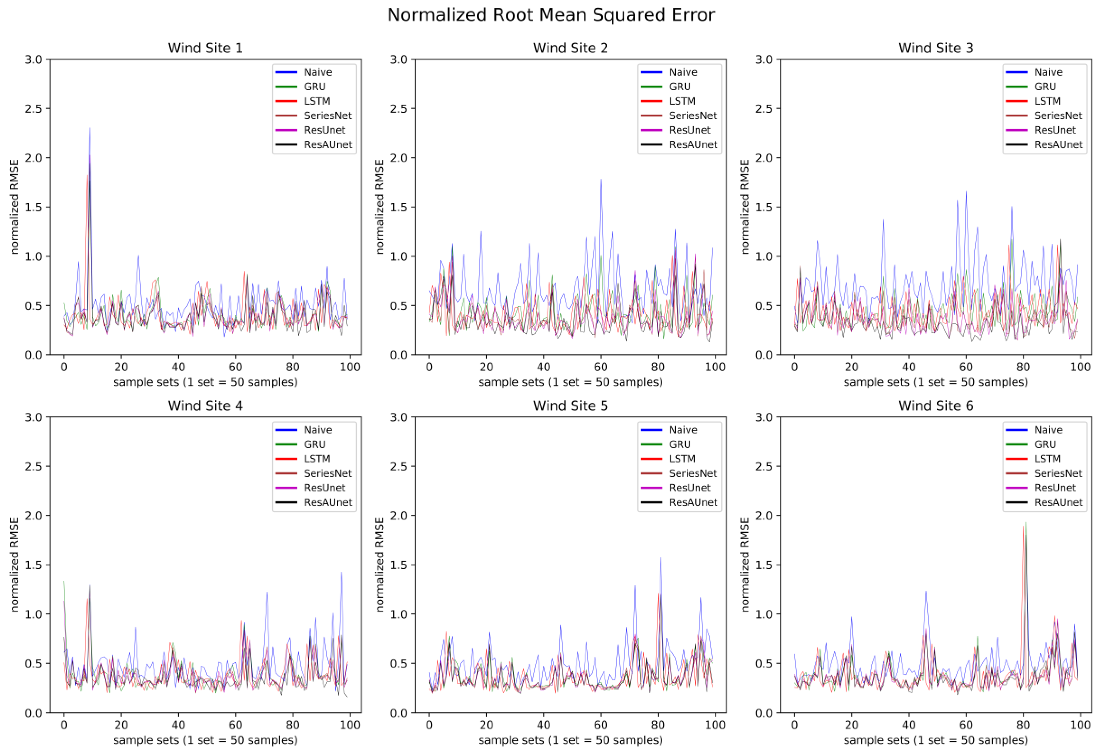
To further verify the performance of ResAUnet, the prediction graphs of each model with corresponding ground truth data for six wind sites are provided in Figure 13, Figure 14, Figure 15, Figure 16, Figure 17 and Figure 18. Moreover, Figure 18 provides the NRMSE of the six models for each prediction step (sample set) on each wind site. The initial 21 sets of timesteps were excluded from the plots since they did not contribute to the evaluation of the models and were only used for training purposes. The plots consist of 5000 timesteps for wind speed. All predictions were made using the out-of-time method, and the model was not trained on the data on which the predictions were made.

Through Figure 13 to Figure 18, the prediction trend of different models was observable. The LSTM and GRU models were able to capture the overall trend of wind speed data. The SeriesNet and ResUnet models evolved over time on the training sets to also capture some of the local trends, which is more visible in Figure 14, Figure 15, and Figure 16. Overall, ResAUnet was able to capture local nonlinear trends much faster and more accurately than the other models. The evolution of ResAUnet could be clearly seen in Figure 13, Figure 14, Figure 15, and Figure 16, where the model was able to follow accurately the local trend of wind speed data much faster than the other models. The NRMSE of each prediction step is plotted in Figure 19, where ResAUnet had the least NRMSE among all models used in this study throughout the validation process.

3.4. Training Time Evaluation

The number of parameters and the models’ architecture had a great influence on the training complexity. For RNN-based models like LSTM and GRU, the recurrent connections increased the training time as the data flow was sequential between the different blocks in the same chain. CNN models, however, did not show this sequential nature of data flow, and all the predictions could be made in parallel. Parallel dataflow enabled CNN models to train faster than their RNN counterparts. We demonstrate the average training time of each model used in the study in

Table 10. Average training time for each training window (in seconds).

Wind Site	LSTM	GRU	SeriesNet	ResUnet	ResAUnet
Site 1	2.45	2.27	0.68	1.34	1.23
Site 2	2.42	2.30	1.19	1.71	1.75
Site 3	2.61	2.11	1.16	1.45	1.63
Site 4	2.45	2.28	0.75	1.25	1.39
Site 5	2.46	2.31	0.72	1.14	1.30
Site 6	2.43	2.28	0.70	1.23	1.44

below.

Experiments were conducted on a notebook PC with an Intel i5 7th generation CPU and 8GB RAM. The TensorFlow API for the Python programming language was used to create and train the models on the notebook’s Nvidia GeForce 920MX dedicated GPU.

4. Conclusions

Improving the accuracy of short-term wind speed prediction is one of the most important factors for improving the energy conversion efficiency. By accurately predicting distant future timesteps (in this case, 50-steps-ahead), efficient power management and planning of repair/cleaning schedules could be done in advance. In this paper, a residual U-net architecture of dilated convolution layers with a nonlinear attention block was proposed for 50-step-ahead prediction of wind speed data using the previous 50 steps. The proposed model was validated using the sliding window technique and was evaluated against several other models including naive prediction. The models were tested on the wind speed data of six different sites. For this study, it could be concluded that:

• CNN architectures consisting of residual blocks made of a dilated convolution layer had higher prediction accuracy than RNN-based architectures like LSTM and GRU. SeriesNet showed an overall performance gain of 3% to 17% for MAPE compared to LSTM, which meant residual blocks of dilated convolution layers were effective for learning wind speed trends without preprocessing the data. Furthermore, CNN architectures required less training time than LSTM and GRU.
• Nonlinear attention blocks applied to the ResAUnet provided an advantage over SeriesNet in predicting wind speed for all wind speed datasets used in this study. ResAUnet performed better on each wind site’s data. A performance gain of up to 17.3% in MAPE, 14.6% in NRMSE, and 15.4% in UMBRAE was observed over the SeriesNet model. Furthermore, ResAUnet could adapt to the local trends in the wind speed data faster than other models used in this study.
• LSTM, GRU, SeriesNet, ResUnet, and ResAUnet could all follow the trend in complex and random wind speed data. However, for 50-step-ahead prediction, dilated convolution-based architectures showed better performance in following the intermediate and local trends. By retraining the model using the sliding window technique, the ResAUnet model adapted to the intermediate trend of the wind speed data faster than the other models.

Overall, the proposed model with nonlinear attention blocks could provide more reliable and accurate 50-step-ahead short-term wind speed prediction for wind farm management systems and improve the efficiency of wind turbine maintenance, cleaning, and operational planning. Even though the proposed model had a clear advantage in 50-step-ahead prediction of short-term wind speed data using raw wind speed data, other environmental factors such as humidity, pressure, wind direction, solar radiation, temperature, and turbulence have great effect on wind speed. Therefore, our future studies will incorporate these influencing factors into multi-step-ahead short-term wind speed prediction. We will also explore other machine learning architectures in order to improve the prediction accuracy.

References

- Tyra, B.; Cassar, C.; Liu, J.; Wong, P.; Yildiz, O. Electric Power Monthly with data for November 2018; U.S. Energy Information Administration: Washington, DC, USA, 2019.
- De Freitas, N.C.A.; Silva, M.P.S.; Sakamoto, M.S. Wind Speed Forecasting: A Review. Int. J. Eng. Res. Appl. 2018, 8, 4–9. [Google Scholar]
- Lei, M.; Shiyan, L.; Chuanwen, J.; Hongling, L.; Yan, Z. A review on the forecasting of wind speed and generated power. Renew. Sustain. Energy Rev. 2009, 13, 915–920. [Google Scholar] [CrossRef]
- George, E.P.; Box, G.M.J. Time Series Analysis: Forecasting and Control; Holden-Day: San Francisco, CA, USA, 1976. [Google Scholar]
- Sim, S.K.; Maass, P.; Lind, P.G. Wind speed modeling by nested ARIMA processes. Energies 2019, 12, 69. [Google Scholar] [CrossRef] [Green Version]
- Lind, P.G.; Vera-Tudela, L.; Wächter, M.; Kühn, M.; Peinke, J. Normal behaviour models for wind turbine vibrations: Comparison of neural networks and a stochastic approach. Energies 2017, 10, 1944. [Google Scholar] [CrossRef] [Green Version]
- More, A.; Deo, M.C. Forecasting wind with neural networks. Mar. Struct. 2003, 16, 35–49. [Google Scholar] [CrossRef]
- Goh, S.L.; Chen, M.; Popović, D.H.; Aihara, K.; Obradovic, D.; Mandic, D.P. Complex-valued forecasting of wind profile. Renew. Energy 2006, 31, 1733–1750. [Google Scholar] [CrossRef]
- El-Fouly, T.H.M.; El-Saadany, E.F.; Salama, M.M.A. One day ahead prediction of wind speed and direction. IEEE Trans. Energy Convers. 2008, 23, 191–201. [Google Scholar] [CrossRef]
- Kulkarni, M.A.; Patil, S.; Rama, G.V.; Sen, P.N. Wind speed prediction using statistical regression and neural network. J. Earth Syst. Sci. 2008, 117, 457–463. [Google Scholar] [CrossRef] [Green Version]
- Chen, N.; Qian, Z.; Meng, X.; Nabney, I.T. Short-term wind power forecasting using Gaussian Processes. IJCAI Int. Jt. Conf. Artif. Intell. 2013, 2790–2796. [Google Scholar]
- Qu, X.; Kang, X.; Chao, Z.; Shuai, J.; Ma, X. Short-term prediction of wind power based on deep Long Short-Term Memory. Asia-Pacific Power Energy Eng. Conf. APPEEC 2016, 2016, 1148–1152. [Google Scholar]
- Raschka, S. Model Evaluation, Model Selection, and Algorithm Selection in Machine Learning. arXiv 2018, arXiv:1811.12808. [Google Scholar]
- Reitermanov, Z. Data Splitting. In Proceedings of the Contributed Papers, Part I—WDS’10, Prague, Czech Republic, 1–4 June 2010; Volume 10, pp. 31–36, ISBN 9788073781392. [Google Scholar]
- Salcedo-Sanz, S.; Ortiz-García, E.G.; Pérez-Bellido, Á.M.; Portilla-Figueras, A.; Prieto, L. Short term wind speed prediction based on evolutionary support vector regression algorithms. Expert Syst. Appl. 2011, 38, 4052–4057. [Google Scholar] [CrossRef]
- Gangwar, S.; Bali, V.; Kumar, A. Comparative Analysis of Wind Speed Forecasting Using LSTM and SVM. ICST Trans. Scalable Inf. Syst. 2018, 159407. [Google Scholar] [CrossRef]
- Shi, X.; Huang, S.; Huang, Q.; Lei, X.; Li, J.; Li, P.; Yang, M. Deep-learning-based Wind Speed Forecasting Considering Spatial–temporal Correlations with Adjacent Wind Turbines. J. Coast. Res. 2019, 93, 623. [Google Scholar] [CrossRef]
- Du, M. Improving LSTM Neural Networks for Better Short-Term Wind Power Predictions. arXiv 2019, arXiv:1907.00489. [Google Scholar]
- Liu, Y.; Guan, L.; Hou, C.; Han, H.; Liu, Z.; Sun, Y.; Zheng, M. Wind power short-term prediction based on LSTM and discrete wavelet transform. Appl. Sci. 2019, 9, 1108. [Google Scholar] [CrossRef] [Green Version]
- Liu, H.; Mi, X.; Li, Y. Smart deep learning based wind speed prediction model using wavelet packet decomposition, convolutional neural network and convolutional long short term memory network. Energy Convers. Manag. 2018, 166, 120–131. [Google Scholar] [CrossRef]
- Ma, Z.; Chen, H.; Wang, J.; Yang, X.; Yan, R.; Jia, J.; Xu, W. Application of hybrid model based on double decomposition, error correction and deep learning in short-term wind speed prediction. Energy Convers. Manag. 2020, 205, 112345. [Google Scholar] [CrossRef]
- Zucatelli, P.J.; Nascimento, E.G.S.; Aylas, G.Y.R.; Souza, N.B.P.; Kitagawa, Y.K.L.; Santos, A.A.B.; Arce, A.M.G.; Moreira, D.M. Short-term wind speed forecasting in Uruguay using computational intelligence. Heliyon 2019, 5, e01664. [Google Scholar] [CrossRef] [Green Version]
- Li, N.; He, F.; Ma, W. Wind power prediction based on extreme learning machine with kernel mean p-power error loss. Energies 2019, 12, 673. [Google Scholar] [CrossRef] [Green Version]
- Qin, Q.; Lai, X.; Zou, J. Direct multistep wind speed forecasting using LSTM neural network combining EEMD and fuzzy entropy. Appl. Sci. 2019, 9, 126. [Google Scholar] [CrossRef] [Green Version]
- Qu, Z.; Zhang, K.; Mao, W.; Wang, J.; Liu, C.; Zhang, W. Research and application of ensemble forecasting based on a novel multi-objective optimization algorithm for wind-speed forecasting. Energy Convers. Manag. 2017, 154, 440–454. [Google Scholar] [CrossRef]
- Huang, C.J.; Kuo, P.H. A short-term wind speed forecasting model by using artificial neural networks with stochastic optimization for renewable energy systems. Energies 2018, 11, 2777. [Google Scholar] [CrossRef] [Green Version]
- Zhao, B.; Lu, H.; Chen, S.; Liu, J.; Wu, D. Convolutional neural networks for time series classification. J. Syst. Eng. Electron. 2017, 28, 162–169. [Google Scholar] [CrossRef]
- Zan, T.; Wang, H.; Wang, M.; Liu, Z.; Gao, X. Application of multi-dimension input convolutional neural network in fault diagnosis of rolling bearings. Appl. Sci. 2019, 9, 2690. [Google Scholar] [CrossRef] [Green Version]
- Cruciani, F.; Vafeiadis, A.; Nugent, C.; Cleland, I.; McCullagh, P.; Votis, K.; Giakoumis, D.; Tzovaras, D.; Chen, L.; Hamzaoui, R. Feature learning for Human Activity Recognition using Convolutional Neural Networks. CCF Trans. Pervasive Comput. Interact. 2020, 2, 18–32. [Google Scholar] [CrossRef] [Green Version]
- Kiranyaz, S.; Avci, O.; Abdeljaber, O.; Ince, T.; Gabbouj, M.; Inman, D.J. 1D Convolutional Neural Networks and Applications: A Survey. arXiv 2019, arXiv:1905.03554. [Google Scholar]
- Huai, N.; Dong, L.; Wang, L.; Hao, Y.; Dai, Z.; Dai, Z.; Dai, Z.; Wang, B. Short-term Wind Speed Prediction Based on CNN_GRU Model. 31th Chinese Control. Decis. Conf. (2019 CCDC) 2019, 1314, 2243–2247. [Google Scholar]
- Wan, R.; Mei, S.; Wang, J.; Liu, M.; Yang, F. Multivariate temporal convolutional network: A deep neural networks approach for multivariate time series forecasting. Electronics 2019, 8, 876. [Google Scholar] [CrossRef] [Green Version]
- Wang, J.H.; Lin, G.F.; Chang, M.J.; Huang, I.H.; Chen, Y.R. Real-Time Water-Level Forecasting Using Dilated Causal Convolutional Neural Networks. Water Resour. Manag. 2019, 33, 3759–3780. [Google Scholar] [CrossRef]
- Geng, Y.; Su, L.; Jia, Y.; Han, C. Seismic Events Prediction Using Deep Temporal Convolution Networks. J. Electr. Comput. Eng. 2019, 2019, 7343784. [Google Scholar] [CrossRef] [Green Version]
- van den Oord, A.; Dieleman, S.; Zen, H.; Simonyan, K.; Vinyals, O.; Graves, A.; Kalchbrenner, N.; Senior, A.; Kavukcuoglu, K. WaveNet: A Generative Model for Raw Audio. arXiv 2016, arXiv:1609.03499. [Google Scholar]
- Heinrich, M.P.; Stille, M.; Buzug, T.M. Residual U-Net convolutional neural network architecture for low-dose CT denoising. Curr. Dir. Biomed. Eng. 2018, 4, 297–300. [Google Scholar] [CrossRef]
- Diakogiannis, F.I.; Waldner, F.; Caccetta, P.; Wu, C. ResUNet-a: A deep learning framework for semantic segmentation of remotely sensed data. ISPRS J. Photogramm. Remote Sens. 2019, 162, 94–114. [Google Scholar] [CrossRef] [Green Version]
- Ni, Z.L.; Bian, G.B.; Zhou, X.H.; Hou, Z.G.; Xie, X.L.; Wang, C.; Zhou, Y.J.; Li, R.Q.; Li, Z. RAUNet: Residual Attention U-Net for Semantic Segmentation of Cataract Surgical Instruments. Lect. Notes Comput. Sci. (including Subser. Lect. Notes Artif. Intell. Lect. Notes Bioinformatics) 2019, 11954 LNCS, 139–149. [Google Scholar]
- Wu, C.; Zou, Y.; Zhan, J. DA-U-Net: Densely Connected Convolutional Networks and Decoder with Attention Gate for Retinal Vessel Segmentation. IOP Conf. Ser. Mater. Sci. Eng. 2019, 533, 012053. [Google Scholar] [CrossRef]
- Oktay, O.; Schlemper, J.; Folgoc, L.L.; Lee, M.; Heinrich, M.; Misawa, K.; Mori, K.; McDonagh, S.; Hammerla, N.Y.; Kainz, B.; et al. Attention U-Net: Learning Where to Look for the Pancreas. arXiv 2018, arXiv:1804.03999. [Google Scholar]
- Shih, S.Y.; Sun, F.K.; Lee, H. yi Temporal pattern attention for multivariate time series forecasting. Mach. Learn. 2019, 108, 1421–1441. [Google Scholar] [CrossRef] [Green Version]
- Zhang, X.; Liang, X.; Zhiyuli, A.; Zhang, S.; Xu, R.; Wu, B. AT-LSTM: An Attention-based LSTM Model for Financial Time Series Prediction. IOP Conf. Ser. Mater. Sci. Eng. 2019, 569, 052037. [Google Scholar] [CrossRef]
- Liu, Y.; Ji, L.; Huang, R.; Ming, T.; Gao, C.; Zhang, J. An attention-gated convolutional neural network for sentence classification. Intell. Data Anal. 2019, 23, 1091–1107. [Google Scholar] [CrossRef] [Green Version]
- Nauta, M.; Bucur, D.; Seifert, C. Causal Discovery with Attention-Based Convolutional Neural Networks. Mach. Learn. Knowl. Extr. 2019, 1, 312–340. [Google Scholar] [CrossRef] [Green Version]
- Hochreiter, S.; Schmidhuber, J. Long Short-Term Memory. Neural Comput. 1997, 9, 1735–1780. [Google Scholar] [CrossRef] [PubMed]
- Steeb, W.-H.; Hardy, Y. Hadamard Product. Probl. Solut. Introd. Adv. Matrix Calc. 2016, 309–317. [Google Scholar]
- Rumelhart, D.E.; Hinton, G.E.; Williams, R.J. Learning representations by back-propagating errors. Nature 1986, 323, 533–536. [Google Scholar] [CrossRef]
- Kingma, D.P.; Ba, J.L. Adam: A method for stochastic optimization. arXiv 2014, arXiv:1412.6980. [Google Scholar]
- Cho, K.; Van Merriënboer, B.; Gulcehre, C.; Bahdanau, D.; Bougares, F.; Schwenk, H.; Bengio, Y. Learning phrase representations using RNN encoder-decoder for statistical machine translation. arXiv 2014, arXiv:1406.1078. [Google Scholar]
- Chung, J.; Gulcehre, C.; Cho, K.; Bengio, Y. Empirical Evaluation of Gated Recurrent Neural Networks on Sequence Modeling. arXiv 2014, arXiv:1412.3555. [Google Scholar]
- Ding, D.; Zhang, M.; Pan, X.; Yang, M.; He, X. Modeling extreme events in time series prediction. Proc. ACM SIGKDD Int. Conf. Knowl. Discov. Data Min. 2019, 1114–1122. [Google Scholar] [CrossRef]
- Aladag, C.H. A new architecture selection method based on tabu search for artificial neural networks. Expert Syst. Appl. 2011, 38, 3287–3293. [Google Scholar] [CrossRef]
- Li, F.; Liu, M.; Zhao, Y.; Kong, L.; Dong, L.; Liu, X.; Hui, M. Feature extraction and classification of heart sound using 1D convolutional neural networks. EURASIP J. Adv. Signal. Process. 2019, 2019, 59. [Google Scholar] [CrossRef] [Green Version]
- Klambauer, G.; Unterthiner, T.; Mayr, A.; Hochreiter, S. Self-normalizing neural networks. Adv. Neural Inf. Process. Syst. 2017, 2017, 972–981. [Google Scholar]
- Kalchbrenner, N.; Espeholt, L.; Simonyan, K.; van den Oord, A.; Graves, A.; Kavukcuoglu, K. Neural Machine Translation in Linear Time. arXiv 2016, arXiv:1610.10099. [Google Scholar]
- Yu, F.; Koltun, V. Multi-scale context aggregation by dilated convolutions. arXiv 2015, arXiv:1511.07122. [Google Scholar]
- Borovykh, A.; Bohte, S.; Oosterlee, C.W. Conditional time series forecasting with convolutional neural networks. Lect. Notes Comput. Sci. (including Subser. Lect. Notes Artif. Intell. Lect. Notes Bioinformatics) 2017, 10614, 729–730. [Google Scholar]
- Borovykh, A.; Bohte, S.; Oosterlee, C.W. Dilated convolutional neural networks for time series forecasting. J. Comput. Financ. 2018, 22. [Google Scholar] [CrossRef] [Green Version]
- He, K.; Zhang, X.; Ren, S.; Sun, J. Deep residual learning for image recognition. Proc. IEEE Comput. Soc. Conf. Comput. Vis. Pattern Recognit. 2016, 2016, 770–778. [Google Scholar]
- Papadopoulos, K. SeriesNet: A Dilated Causal Convolutional Neural Network for Forecasting. In Proceedings of the International Conference on Pattern Recognition and Machine Intelligence, Union, NJ, USA, 1–4 August 2018; pp. 1–22. [Google Scholar]
- Ronneberger, O.; Fischer, P.; Brox, T. U-net: Convolutional networks for biomedical image segmentation. Lect. Notes Comput. Sci. (including Subser. Lect. Notes Artif. Intell. Lect. Notes Bioinformatics) 2015, 9351, 234–241. [Google Scholar]
- Zhang, Z.; Liu, Q.; Wang, Y. Road Extraction by Deep Residual U-Net. IEEE Geosci. Remote Sens. Lett. 2018, 15, 749–753. [Google Scholar] [CrossRef] [Green Version]
- Yu, B.; Yin, H.; Zhu, Z. ST-UNet: A Spatio-Temporal U-Network for Graph-structured Time Series Modeling. arXiv 2019, arXiv:1903.05631. [Google Scholar]
- Ranzato, M.; Huang, F.J.; Boureau, Y.L.; LeCun, Y. Unsupervised learning of invariant feature hierarchies with applications to object recognition. Proc. IEEE Comput. Soc. Conf. Comput. Vis. Pattern Recognit. 2007, 1–8. [Google Scholar] [CrossRef] [Green Version]
- Lai, G.; Chang, W.C.; Yang, Y.; Liu, H. Modeling long- and short-term temporal patterns with deep neural networks. 41st Int. ACM SIGIR Conf. Res. Dev. Inf. Retrieval SIGIR 2018 2018, 95–104. [Google Scholar] [CrossRef] [Green Version]
- Cinar, Y.G.; Mirisaee, H.; Goswami, P.; Gaussier, E.; Aït-Bachir, A.; Strijov, V. Position-based content attention for time series forecasting with sequence-to-sequence RNNs. Lect. Notes Comput. Sci. (including Subser. Lect. Notes Artif. Intell. Lect. Notes Bioinformatics) 2017, 10638, 533–544. [Google Scholar]
- Ran, X.; Shan, Z.; Fang, Y.; Lin, C. An LSTM-based method with attention mechanism for travel time prediction. Sensors 2019, 19, 861. [Google Scholar] [CrossRef] [PubMed] [Green Version]
- Zhu, Y.; Sun, W.; Cao, X.; Wang, C.; Wu, D.; Yang, Y.; Ye, N. TA-CNN: Two-way attention models in deep convolutional neural network for plant recognition. Neurocomputing 2019, 365, 191–200. [Google Scholar] [CrossRef]
- Chen, Y.; Kalantidis, Y.; Li, J.; Yan, S.; Feng, J. A2-Nets: Double attention networks. Adv. Neural Inf. Process. Syst. 2018, 2018, 352. [Google Scholar]
- Song, H.; Rajan, D.; Thiagarajan, J.J.; Spanias, A. Attend and diagnose: Clinical time series analysis using attention models. In Proceedings of the 32nd AAAI Conference on Artificial Intelligence. AAAI, New Orleans, LA, USA, 2–7 February 2018; Volume 2018, pp. 4091–4098, ISBN 9781577358008. [Google Scholar]
- Bharani, R.; Sivaprakasam, A. A large volume wind data for renewable energy applications. Data Br. 2019, 25, 104291. [Google Scholar] [CrossRef]
- Hu, B.; Li, Y.; Yang, H.; Wang, H. Wind speed model based on kernel density estimation and its application in reliability assessment of generating systems. J. Mod. Power Syst. Clean Energy 2017, 5, 220–227. [Google Scholar] [CrossRef] [Green Version]
- Diebold, F.X.; Mariano, R.S. Comparing predictive accuracy. J. Bus. Econ. Stat. 2002, 20, 134–144. [Google Scholar] [CrossRef]
- Giacomini, R.; White, H. Tests of Conditional Predictive Ability. Econometrica 2006, 74, 1545–1578. [Google Scholar] [CrossRef] [Green Version]
- Yu, Y.; Zhu, Y.; Li, S.; Wan, D. Time series outlier detection based on sliding window prediction. Math. Probl. Eng. 2014, 2014. [Google Scholar] [CrossRef]
- Vafaeipour, M.; Rahbari, O.; Rosen, M.A.; Fazelpour, F.; Ansarirad, P. Application of sliding window technique for prediction of wind velocity time series. Int. J. Energy Environ. Eng. 2014, 5, 1–7. [Google Scholar] [CrossRef] [Green Version]
- Mozaffari, L.; Mozaffari, A.; Azad, N.L. Vehicle speed prediction via a sliding-window time series analysis and an evolutionary least learning machine: A case study on San Francisco urban roads. Eng. Sci. Technol. Int. J. 2015, 18, 150–162. [Google Scholar] [CrossRef] [Green Version]
- Hota, H.S.; Handa, R.; Shrivas, A.K. Time Series Data Prediction Using Sliding Window Based RBF Neural Network. Int. J. Comput. Intell. Res. 2017, 13, 1145–1156. [Google Scholar]
- Makridakis, S. The M3-Competition: Results, conclusions and implications. Int. J. Forecast. 2000, 16, 451–476. [Google Scholar] [CrossRef]
- Chen, C.; Twycross, J.; Garibaldi, J.M. A new accuracy measure based on bounded relative error for time series forecasting. PLoS ONE 2017, 12, e0174202. [Google Scholar] [CrossRef] [Green Version]
Figure 1.
Structure of an LSTM network, where LSTM cells are linked as a chain. For each LSTM cell, x and h are the input and output, respectively.
Figure 2.
A gated recurrent unit.
Figure 3.
(a) Stacked LSTM model with two hidden LSTM layers followed by an FC layer; (b) stacked gated recurrent unit (GRU) model with two hidden GRU layers followed by an FC layer.
Figure 4.
One-dimensional CNN structure with (a) standard convolution, (b) causal convolution, and (c) dilated causal convolution.
Figure 5.
(a) Residual dilated convolution block with ReLU activation and a dropout layer. (b) Self-normalizing residual block with scaled exponential linear unit (SELU) activation and skipped connection.
Figure 6.
SeriesNet with residual blocks and skipped connections.
Figure 7.
Residual U-Net (ResUnet) architecture for wind series time series prediction.
Figure 8.
Non-Linear attention blocked with fully connected layers.
Figure 9.
Residual attention U-Net with the proposed nonlinear attention block.
Figure 10.
Probability distribution of wind speed at different data collection sites.
Figure 11.
Sliding window validation method for time series prediction models.
Figure 12.
Training and prediction method.
Figure 13.
Prediction results of the six models for wind Site 1.
Figure 14.
Prediction results of the six models for wind Site 2.
Figure 15.
Prediction results of the six models for wind Site 3.
Figure 16.
Prediction results of the six models for wind Site 4.
Figure 17.
Prediction results of the six models for wind Site 5.
Figure 18.
Prediction results of the six models for wind Site 6.
Figure 19.
NRMSE of the six models for different wind sites at each prediction step (sample set).