Investigation on the Effects of Magnetic Saturation in Six-Phase Induction Machines with and without Cross Saturation of the Main Flux Path

Abstract

The operational characteristics during transients are significantly influenced by magnetic saturation in electrical equipment. For the computation of steady-state rated operation in multiphase induction machines, the assumption of linear magnetic behavior of the iron core in classical machine models may be sufficient. The mathematical models of the considered models differ in terms of the existence or absence of dynamic cross-saturation effects. The approach that is most frequently used to examine the impact of magnetic saturation is based on the state-space variable representation of the mathematical model in dynamic axes (d–q). The purpose of this research is to investigate the effects of magnetic saturation on six-phase induction machines. In this study, a d–q transformation-based model of a six-phase induction machine (SPIM), including the magnetic saturation effect, is developed. The cross-saturation and the common mutual leakage inductance between the two sets of stators’ windings are then developed and analyzed, and the developed models were simulated and results are compared with and without cross-saturation. The main and leakage flux saturation, as well as the mutual coupling between the two windings, are all accounted for in the model, which is based on the vector space decomposition method. A significant increase in currents and voltage results from the highly saturated magnetic paths of the leakage fluxes in six-phase induction machines. In order to investigate the impact of cross-saturation, inductances computed using analytical methods and those without taking cross-saturation into consideration were compared. These outcomes are then transformed into a condensed current depending on parameter functions for transient machine models.

1. Introduction

Multiphase induction machines are widely used in various fields and for a wide range of energy conversion. The stand-alone asynchronous generator has emerged as a suitable contender in isolated power sources [1,2]. Due to their benefits over traditional three-phase systems, multiphase electric drives are promoted as industrial solutions for high-demand applications. A better power distribution per phase, an increase in reliability, and the availability of additional freedom degrees should be highlighted among these advantages. Due to the drawbacks of the three-phase system, the multiphase induction machines are conceived. Investigation shows that the six-phase induction machine is more advantageous compared to the three-phase counterpart [3,4,5].

By using a number of phases greater than three in the power transmission, the noise level is considerably reduced. Consequently, a multi-phase line with small dimensions can be used to transmit large powers covering a complete voltage range [6,7]. Due to its potential benefits from using a greater than three-phase order system in power transmission, there has also been a growing interest in six-phase induction machines. Modern power systems can benefit from the use of multiphase electrical machines for a variety of purposes, including wind energy conversion, electric vehicles, airplanes, and high power industrial motors [8,9,10,11].

Generally, during the analytical modelling of the six-phase induction machines, one uses a linear model, which neglects the effect of the magnetic saturation. It is then assumed that the magnetizing characteristic ${\lambda }_m(i_m)$ is linear, but the behavior of the six-phase induction machines is no longer reproduced correctly when the saturation effects are no longer negligible. Whatever model is used, adequate magnetic circuit saturation modelling is necessary for obtaining satisfactory simulation accuracy and control performance. Typically, electrical machines work in the saturated region to provide more torque [12,13,14,15]. It is suggested that the machine designer precisely model the electrical machine before setting the restrictions. This is crucial, especially when the modelling takes into consideration actual operational conditions, and especially taking account the magnetic saturation [16,17,18,19].

In addition, the nominal operating points of the six-phase induction machines are located in the saturated zone and with a view to extracting maximum power from it at a reasonable cost. Consequently, taking magnetic saturation into account is not dictated by the concern to improve the results, but it can sometimes be a necessity [20,21,22,23].

Introducing the magnetic nonlinearities into the equations of operation in any regime is to cross an additional level in the modelling. The philosophy adopted considers the inherent flux of a winding as the superposition of a leakage flux closing in the air and a useful flux traversing the magnetic circuit, the stator and rotor leakage inductances being constant. This implies that only the mutual fluxes are subject to saturation of the magnetic circuit [24,25,26].

We begin this paper with a description of the equations of operation of the six-phase induction machines (SPIM) in the natural reference and then the Park reference. Then, the work will be entirely devoted to the multiplicity of the d–q models of the six-phase induction machines; on the other hand, there is the introduction of the magnetic saturation in the modelling of the six-phase induction machines. Indeed, by a suitable choice of the state variables among the characteristic space vectors, we will develop the two flux and current models, including the magnetic saturation in the of the main flux path. After that is the introduction of magnetic saturation, where the winding currents’ model incorporating saturation is elaborated and followed by a description of the method for deriving the remaining models. Derivation of some selected models will be detailed. Hence, the saturation effect is considered and included in the saturated model. Simulation results will be provided to examine the impact of magnetic saturation, considering the stator currents and magnetization flux in the (d–q) axis as state variables. Finally, simulation results will be compared with and without cross-saturation, which consider mitigation of the magnetic saturation effect.

2. Six-Phase Induction Machine Model in The Rotor Reference Frame

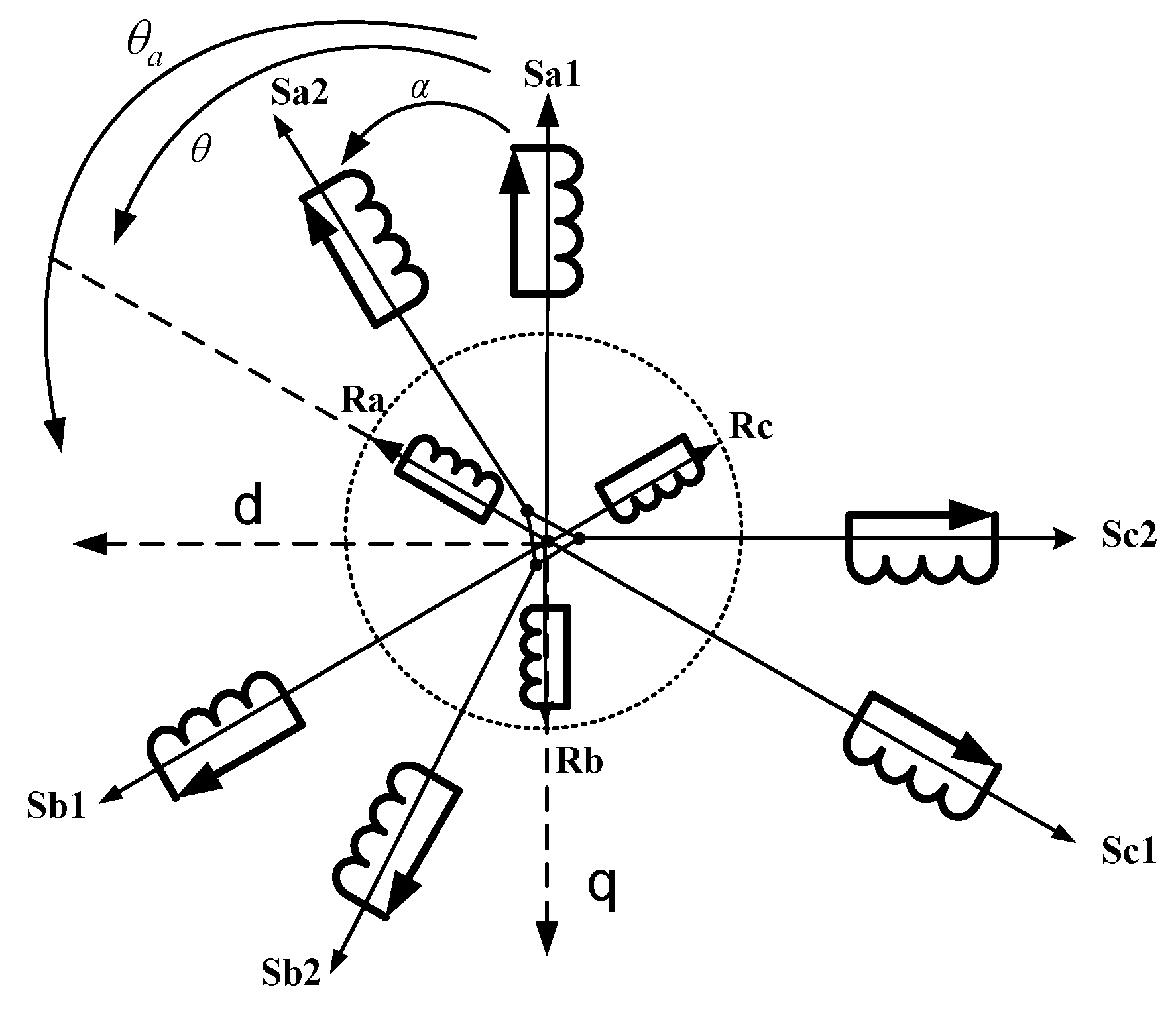
In the mathematical description of a dual stator induction motor, it is assumed that the six-phase induction machine (SPIM) is considered as an electromechanical system consisting of two three-phase stator windings, denoted as stator 1 and stator 2, and the common squirrel-cage rotor winding. The cage rotor winding is replaced by an equivalent three-phase winding. Figure 1 shows the representation of the stator and rotor windings of a dual stator induction motor.

A common type of multiphase machine is the six-phase induction motor (SPIM), where two sets of three-phase windings, spatially phase shifted by 30 electrical degrees, share a common stator magnetic core.

With:

${\mathsf{\theta }}_{\mathrm{a}}$: expresses the angle of displacement between star 1 and axis d.

$\mathsf{\theta }$: expresses the angle of displacement between star 1 and the rotor.

$\mathsf{\alpha }$: expresses the offset angle between the two stars.

We can define the modeling of a given system as being the search for a mathematical representation capable of identifying with its behavior. This representation can appear in practice in two different aspects: (i) Static model: concerns the static aspect of the system, which implies its operation in a steady state. It is established from steady state equations and energy balances. (ii) Dynamic model: consumed by the dynamic aspect of the system. It is obtained from differential equations in instantaneous magnitudes, developed on the basis of a physical approach to the system.

By writing Faraday’s law for each of the windings, the voltage equations for the six stator phases and the three dynamic rotor phases can be written as follows:

$$\left[V_{s1}\right]=R_{s1}\left[i_{s1}\right]+\frac{d}{dt}\left[{\lambda }_{s1}\right]\hspace{0.17em}$$

(1)

$$\left[V_{s2}\right]=R_{s2}\left[i_{s2}\right]+\frac{d}{dt}\left[{\lambda }_{s2}\right]\hspace{0.17em}\hspace{0.17em}\hspace{0.17em}\hspace{0.17em}$$

(2)

$$\left[V_r\right]=R_r\left[i_r\right]+\frac{d}{dt}\left[{\lambda }_r\right]\hspace{0.17em}$$

(3)

With:

$$\left[V_{s1}\right]={\left[\begin{array}{ccc}{v}_{as1}& v_{bs1}& v_{cs1}\end{array}\right]}^t,\hspace{0.17em}\hspace{0.17em}\hspace{0.17em}\hspace{0.17em}\hspace{0.17em}\hspace{0.17em}\hspace{0.17em}\left[i_{s1}\right]={\left[\begin{array}{ccc}{i}_{as1}& i_{bs1}& i_{cs1}\end{array}\right]}^t\hspace{0.17em}et\hspace{0.17em}\left[{\lambda }_{s1}\right]={\left[\begin{array}{ccc}{\lambda }_{as1}& {\lambda }_{bs1}& {\lambda }_{cs1}\end{array}\right]}^t$$

(4)

$$\left[V_{s2}\right]={\left[\begin{array}{ccc}{v}_{as2}& v_{bs2}& v_{cs2}\end{array}\right]}^t,\hspace{0.17em}\hspace{0.17em}\hspace{0.17em}\hspace{0.17em}\hspace{0.17em}\hspace{0.17em}\left[i_{s2}\right]={\left[\begin{array}{ccc}{i}_{as2}& i_{bs2}& i_{cs2}\end{array}\right]}^t\hspace{0.17em}et\hspace{0.17em}\left[{\lambda }_{s2}\right]={\left[\begin{array}{ccc}{\lambda }_{as2}& {\lambda }_{bs2}& {\lambda }_{cs2}\end{array}\right]}^t$$

(5)

$$\left[V_r\right]={\left[v_{ar\hspace{0.17em}\hspace{0.17em}\hspace{0.17em}\hspace{0.17em}\hspace{0.17em}\hspace{0.17em}\hspace{0.17em}\hspace{0.17em}}{v}_{br\hspace{0.17em}\hspace{0.17em}\hspace{0.17em}\hspace{0.17em}\hspace{0.17em}\hspace{0.17em}\hspace{0.17em}\hspace{0.17em}}{v}_{cr\hspace{0.17em}\hspace{0.17em}\hspace{0.17em}\hspace{0.17em}\hspace{0.17em}\hspace{0.17em}\hspace{0.17em}\hspace{0.17em}}\right]}^t,\hspace{0.17em}\hspace{0.17em}\hspace{0.17em}\hspace{0.17em}\hspace{0.17em}\hspace{0.17em}\hspace{0.17em}\left[{\lambda }_r\right]={\left[{\lambda }_{ar\hspace{0.17em}\hspace{0.17em}\hspace{0.17em}\hspace{0.17em}\hspace{0.17em}\hspace{0.17em}\hspace{0.17em}\hspace{0.17em}}{\lambda }_{br\hspace{0.17em}\hspace{0.17em}\hspace{0.17em}\hspace{0.17em}\hspace{0.17em}\hspace{0.17em}\hspace{0.17em}\hspace{0.17em}}{\lambda }_{cr\hspace{0.17em}\hspace{0.17em}\hspace{0.17em}\hspace{0.17em}\hspace{0.17em}\hspace{0.17em}\hspace{0.17em}\hspace{0.17em}}\right]}^t\hspace{0.17em}\hspace{0.17em}\hspace{0.17em}\hspace{0.17em}et\hspace{0.17em}\hspace{0.17em}\hspace{0.17em}\hspace{0.17em}\left[i_r\right]={\left[i_{ar\hspace{0.17em}\hspace{0.17em}\hspace{0.17em}\hspace{0.17em}\hspace{0.17em}\hspace{0.17em}\hspace{0.17em}\hspace{0.17em}}{i}_{br\hspace{0.17em}\hspace{0.17em}\hspace{0.17em}\hspace{0.17em}\hspace{0.17em}\hspace{0.17em}\hspace{0.17em}\hspace{0.17em}}{i}_{cr\hspace{0.17em}\hspace{0.17em}\hspace{0.17em}\hspace{0.17em}\hspace{0.17em}\hspace{0.17em}\hspace{0.17em}\hspace{0.17em}}\right]}^t$$

(6)

$\left[V_{s1}\right],\hspace{0.17em}\hspace{0.17em}\left[V_{s2}\right]$: Stator1 and stator2 voltage vectors.

$\left[i_{s1}\right],\hspace{0.17em}\hspace{0.17em}\left[i_{s2}\right]$: Stator1 and stator2 current vectors.

$\left[{\lambda }_{s1}\right],\hspace{0.17em}\hspace{0.17em}\left[{\lambda }_{s2}\right]$: Stator1 and stator2 flux vectors.

$\left[V_r\right]$: Rotor voltage vectors.

$\left[i_r\right]$: Rotor current vectors.

$\left[{\lambda }_r\right]$: Rotor flux vectors.

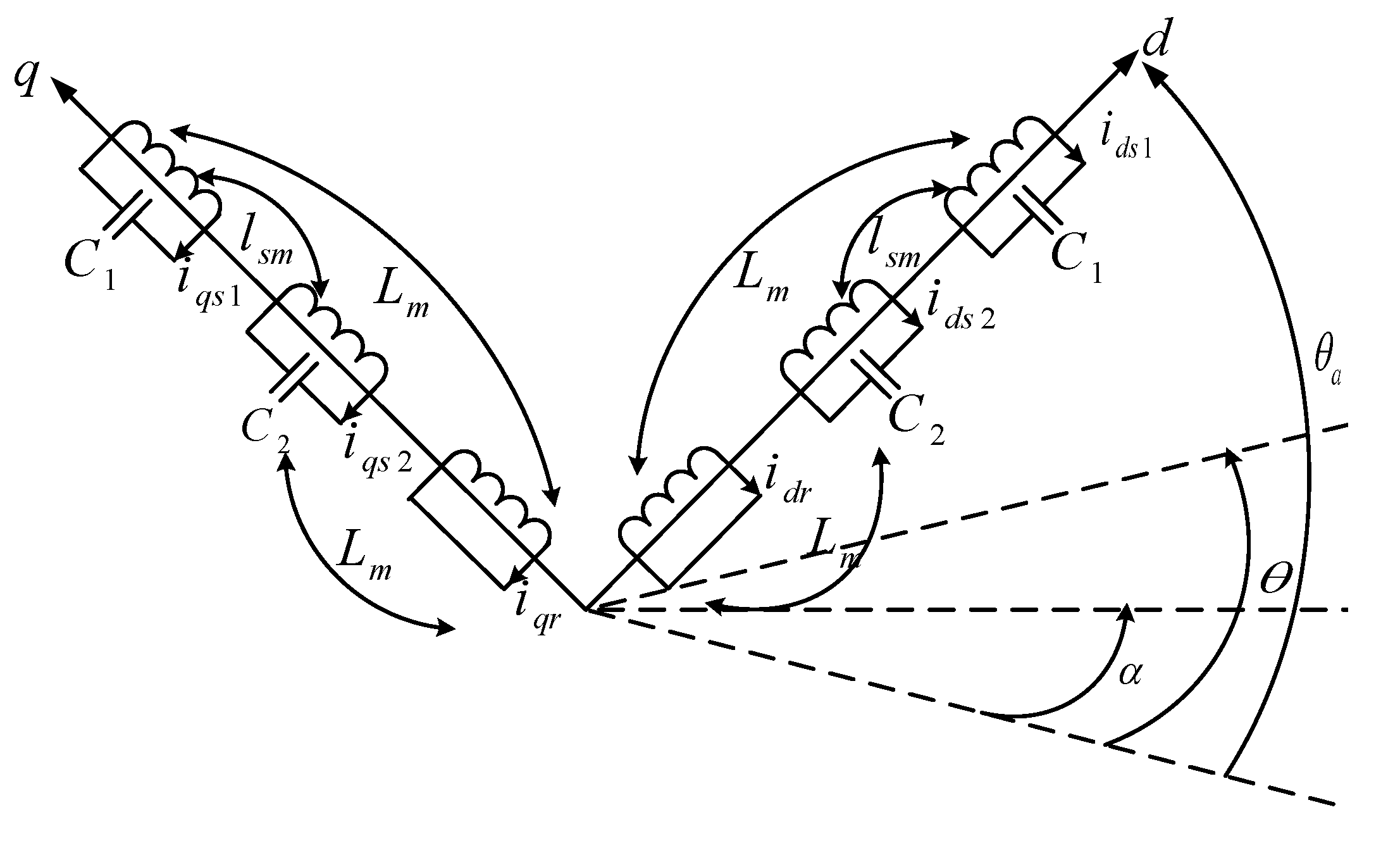
The equivalent electrical model of the generator in Park’s frame is shown in Figure 2. In this benchmark, we obtain a relative model where the SPIM is represented by two coupled electrical circuits, one along the direct axis d and the other along the quadrature axis q.

The voltage equations of the SPIM using decomposition vector space are as follows. For the stator circuit, we can write:

$$\left\{\begin{array}{l}{V}_{ds1}=R_s.i_{ds1}+\frac{d{\lambda }_{ds1}}{dt}-w_a{\lambda }_{qs1}\\ V_{qs1}=R_s.i_{qs1}+\frac{d{\lambda }_{qs1}}{dt}+w_a{\lambda }_{ds1}\\ V_{ds2}=R_s.i_{ds2}+\frac{d{\lambda }_{ds2}}{dt}-w_a{\lambda }_{qs2} \\ V_{qs2}=R_s.i_{qs2}+\frac{d{\lambda }_{qs2}}{dt}+w_a{\lambda }_{ds2}\end{array}\right.$$

(7)

Further, for the rotor circuit, we have:

$$\left\{\begin{array}{l}0=R_r.i_{dr}+\frac{d{\lambda }_{dr}}{dt}-(w_a-w){\lambda }_{qr}\\ 0=R_r.i_{qr}+\frac{d{\lambda }_{qr}}{dt}+(w_a-w){\lambda }_{dr}\end{array}\right.$$

(8)

where $w_a$ is the speed of the reference frame.

The expressions of stator and rotor flux linkages are:

$$\left\{\begin{array}{c}{\lambda }_{ds1}=\left(l_s+l_{sm}+L_{dm}\right)i_{ds1}+\left(l_{sm}+L_{dm}\right)i_{ds2}+L_{dm}{i}_{dr}\hfill \\ {\lambda }_{qs1}=\left(l_s+l_{sm}+L_{qm}\right)i_{qs1}+\left(l_{sm}+L_{qm}\right)i_{qs2}+L_{qm}{i}_{qr}\hfill \\ {\lambda }_{ds2}=\left(l_s+L_{dm}\right)i_{ds1}+\left(l_s+l_{sm}+L_{dm}\right)i_{ds2}+L_{dm}{i}_{dr}\hfill \\ {\lambda }_{qs2}=\left(l_{sm}+L_{qm}\right)i_{qs1}+\left(l_s+l_{sm}+L_{qm}\right)i_{qs2}+L_{qm}{i}_{dr}\hfill \\ {\lambda }_{dr}=L_{dm}{i}_{ds1}+L_{dm}{i}_{ds1}+\left(l_r+L_{dm}\right)i_{dr}\hfill \\ {\lambda }_{qr}=L_{qm}{i}_{qs1}+L_{qm}{i}_{qs2}+\left(l_r+L_{qm}\right)i_{qr}\hfill \end{array}\right.$$

(9)

where $l_{sm}$ is the common mutual leakage inductance between the two sets of stators windings, $L_m$ is the mutual inductance between stator and rotor, and $l_s,l_r$ are the stator and rotor leakage inductance, respectively.

Where:

$$\left\{\begin{array}{l}{L}_s=l_s+l_{sm}+L_m \\ L_r=l_r+L_m \\ L_{ps}=l_{sm}+L_m \\ M=L_m\end{array}\right.$$

(10)

With:

$$\left\{\begin{array}{l}\frac{d{\lambda }_{dm}}{dt}=\frac{d{\lambda }_{dm}}{d{i}_{dm}}\frac{d{i}_{dm}}{dt}=L_{dmdy}\frac{d}{dt}\left(i_{ds1}+i_{ds2}+i_{dr}\right)\\ \frac{d{\lambda }_{qm}}{dt}=\frac{d{\lambda }_{qm}}{d{i}_{qm}}\frac{d{i}_{qm}}{dt}=L_{qmdy}\frac{d}{dt}\left(i_{qs1}+i_{qs2}+i_{qr}\right)\end{array}\right.$$

(11)

The writing matrix of flux is characterized by the following relationship:

$$\left\{\begin{array}{l}\left[V\right]=\left[A\right]\left[\dot{X}\right]+\left[B\right]\left[X\right]\\ \left[V\right]={\left[\begin{array}{cccccc}{V}_{ds1}& V_{qs1}& V_{ds2}& V_{qs2}& 0& 0\end{array}\right]}^t\\ \left[X\right]={\left[\begin{array}{cccccc}{i}_{ds1}& i_{qs1}& i_{ds2}& i_{qs2}& i_{dr}& i_{qr}\end{array}\right]}^t\end{array}\right.$$

(12)

$$\left[A\hspace{0.17em}\hspace{0.17em}\right]=\left[\begin{array}{cccccc}{l}_s+l_{s\hspace{0.17em}m}\hspace{0.17em}\hspace{0.17em}+L_{dmdy}& 0& l_{sm}+L_{dmdy}& 0& L_{dmdy}& 0\\ 0& l_s+l_{s\hspace{0.17em}m}+L_{qmdy}& 0& l_{s\hspace{0.17em}m}+L_{qmdy}& 0& L_{qmdy}\\ l_{s\hspace{0.17em}m}+L_{dmdy}& 0& l_s+l_{s\hspace{0.17em}m}+L_{dmdy}& 0& L_{dmdy}& 0\\ 0& l_{s\hspace{0.17em}m}+L_{qmdy}& 0& l_s+l_{s\hspace{0.17em}m}+\hspace{0.17em}\hspace{0.17em}{L}_{qmdy}& 0& L_{qmdy}\\ L_{dmdy}& 0& L_{dmdy}& 0& l_r+\hspace{0.17em}\hspace{0.17em}{L}_{dmdy}& 0\\ 0& L_{qmdy}& 0& L_{qmdy}& 0& l_r+\hspace{0.17em}\hspace{0.17em}{L}_{qmdy}\end{array}\right]$$

(13)

$$\left[B\right]=\left[\begin{array}{cccccc}{R}_s& 0& 0& 0& 0& 0\\ 0& R_s& 0& 0& 0& 0\\ 0& 0& R_s& 0& 0& 0\\ 0& 0& 0& R_s& 0& 0\\ 0& L_{qm}\hspace{0.17em}\hspace{0.17em}{w}_e& 0& L_{qm}\hspace{0.17em}\hspace{0.17em}{w}_e& R_r& (l_r+L_{qm})\hspace{0.17em}\hspace{0.17em}{w}_e\\ -L_{dm}\hspace{0.17em}\hspace{0.17em}{w}_e& 0& -L_{dm}\hspace{0.17em}\hspace{0.17em}{w}_e& 0& -(l_r+L_{dm})\hspace{0.17em}\hspace{0.17em}{w}_e& R_r\end{array}\right]$$

(14)

The analytical d-model has been developed in a general reference frame and can be used to analyze the behavior of the induction machine in any reference frame.

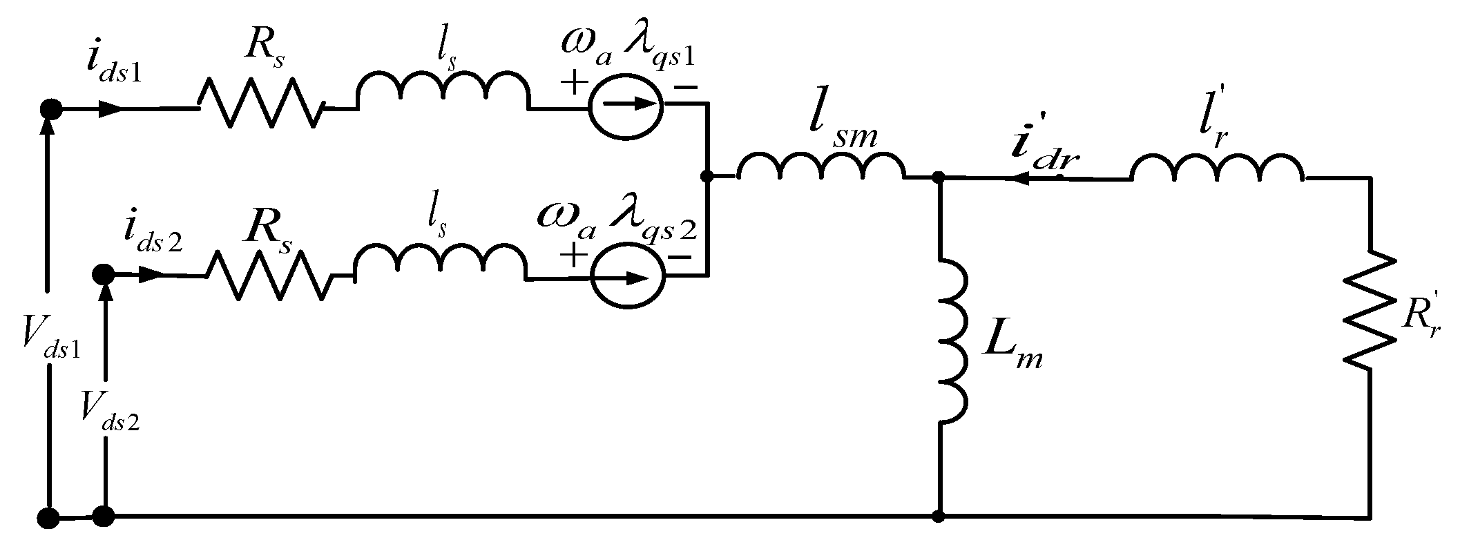
These equations suggest the equivalent circuit, as shown in Figure 3. The common mutual leakage inductance represents the fact that the two sets of stator windings occupy the same slots and are, therefore, mutually coupled by a component of leakage flux.

3. Multiplicity of D–Q Models of the Six-Phase Induction Machine

In terms of space vectors, we can rewrite the main system (7) in the form:

$$\left\{\begin{array}{l}{\overline{v}}_{s1}=R_s{\overline{i}}_{s1}+\frac{d{\overline{\lambda }}_{s1}}{dt}+j{w}_a{\overline{\lambda }}_{s1}\\ {\overline{v}}_{s2}=R_s{\overline{i}}_{s2}+\frac{d{\overline{\lambda }}_{s2}}{dt}+j{w}_a{\overline{\lambda }}_{s2}\\ {\overline{v}}_r=R_r{\overline{i}}_r+\frac{d{\overline{\lambda }}_r}{dt}+j(w_a-w_e){\overline{\lambda }}_r \end{array}\right.$$

(15)

The rotor winding is usually shorted, either ${\overline{v}}_r=\hspace{0.33em}0$.

Whatever the regime and the operating mode, the resolution of the differential system (7) requires three vectors that can be identified from the flux equations. On the other hand, the examination of this system and its annexed relations (8)–(9) makes it possible to identify the possible state variables in terms of space vectors, which are $\hspace{0.17em}{\overline{i}}_{s1},\hspace{0.17em}\hspace{0.17em}{\overline{i}}_{s2},\hspace{0.17em}\hspace{0.17em}\hspace{0.17em}{\overline{i}}_r\hspace{0.17em}\hspace{0.17em},\hspace{0.17em}\hspace{0.17em}{\overline{\lambda }}_{s1},\hspace{0.17em}\hspace{0.17em}{\overline{\lambda }}_{s2},$ and $\hspace{0.17em}\hspace{0.17em}{\overline{\lambda }}_r$. The selection of three vectors among this set provides the total number of possible models for a double star asynchronous machine.

However, referring to the differential system (15), three direct components and three quadrature components suffice. In other words, three vectors solve the problem. To this end, the choice of state variables can be made as follows: Selecting three vectors from the set of six vectors $(\hspace{0.17em}{\overline{i}}_{s1},\hspace{0.17em}\hspace{0.17em}{\overline{i}}_{s2},\hspace{0.17em}\hspace{0.17em}\hspace{0.17em}{\overline{i}}_r\hspace{0.17em}\hspace{0.17em},\hspace{0.17em}\hspace{0.17em}{\overline{\lambda }}_{s1},\hspace{0.17em}\hspace{0.17em}{\overline{\lambda }}_{s2},{\overline{\lambda }}_r)$ supplies the total number of possible models for a double-star asynchronous machine, so the effective number of models is $C_6^3=20$ models.

We can sort and classify all the models thus obtained according to the nature of the state variables, which are obviously currents and/or fluxes. This results in the definition of three families of models: current models, flow models, and mixed models. Then, the objective in what follows is to develop two models among the most used in the literature, such as the winding current model $({\overline{i}}_{s1},{\overline{i}}_{s2},{\overline{i}}_r)$ and the pure flux model $({\overline{\lambda }}_{s1},{\overline{\lambda }}_{s2},{\overline{\lambda }}_r)$ for the SPIM.

All the models of a SPIM thus found are summarized below in families and according to the state variables.

• Current model: $(\hspace{0.17em}{\overline{i}}_{s1},\hspace{0.17em}\hspace{0.17em}{\overline{i}}_{s2},\hspace{0.17em}\hspace{0.17em}\hspace{0.17em}{\overline{i}}_r)$
• Flux model $({\overline{\lambda }}_{s1},\hspace{0.17em}\hspace{0.17em}{\overline{\lambda }}_{s2},{\overline{\lambda }}_r)$
• 18 mixed models, which can be defined in two categories of models:

  -

  9 models using two current vectors and one flux vector,

  $$(\hspace{0.17em}{\overline{i}}_{s1},\hspace{0.17em}\hspace{0.17em}{\overline{i}}_{s2},\hspace{0.17em}\hspace{0.17em}{\overline{\lambda }}_{s1}),\hspace{0.17em}(\hspace{0.17em}{\overline{i}}_{s1},\hspace{0.17em}\hspace{0.17em}{\overline{i}}_{s2},\hspace{0.17em}\hspace{0.17em}{\overline{\lambda }}_{s2}),\hspace{0.17em}(\hspace{0.17em}{\overline{i}}_{s1},\hspace{0.17em}\hspace{0.17em}{\overline{i}}_{s2},\hspace{0.17em}\hspace{0.17em}{\overline{\lambda }}_r)$$

  $$(\hspace{0.17em}{\overline{i}}_{s1},\hspace{0.17em}\hspace{0.17em}{\overline{i}}_r\hspace{0.17em}\hspace{0.17em},\hspace{0.17em}\hspace{0.17em}{\overline{\lambda }}_{s1}),\hspace{0.17em}(\hspace{0.17em}{\overline{i}}_{s1},{\overline{i}}_r\hspace{0.17em}\hspace{0.17em},{\overline{\lambda }}_{s2}),\hspace{0.17em}(\hspace{0.17em}{\overline{i}}_{s1},{\overline{i}}_r\hspace{0.17em}\hspace{0.17em},{\overline{\lambda }}_r)$$

  $$({\overline{i}}_{s2},\hspace{0.17em}\hspace{0.17em}{\overline{i}}_r,\hspace{0.17em}\hspace{0.17em}{\overline{\lambda }}_{s1}),\hspace{0.17em}({\overline{i}}_{s2},\hspace{0.17em}\hspace{0.17em}{\overline{i}}_r,{\overline{\hspace{0.17em}\hspace{0.17em}\lambda }}_{s2}),\hspace{0.17em}({\overline{i}}_{s2},\hspace{0.17em}\hspace{0.17em}{\overline{i}}_r\hspace{0.17em}\hspace{0.17em},\hspace{0.17em}\hspace{0.17em}{\overline{\lambda }}_r)$$

  -

  9 models using two flux vectors and one current vector,

  $$(\hspace{0.17em}{\overline{i}}_{s1},{\overline{\lambda }}_{s1},\hspace{0.17em}\hspace{0.17em}{\overline{\lambda }}_{s2}),\hspace{0.17em}(\hspace{0.17em}{\overline{i}}_{s1},\hspace{0.17em}\hspace{0.17em}{\overline{\lambda }}_{s1},{\overline{\lambda }}_r),\hspace{0.17em}(\hspace{0.17em}{\overline{i}}_{s1},\hspace{0.17em}\hspace{0.17em}{\overline{\lambda }}_{s2},{\overline{\lambda }}_r)$$

  $$({\overline{i}}_{s2},\hspace{0.17em}{\overline{\lambda }}_{s1},\hspace{0.17em}\hspace{0.17em}{\overline{\lambda }}_{s2}),\hspace{0.17em}({\overline{i}}_{s2},\hspace{0.17em}\hspace{0.17em}{\overline{\lambda }}_{s1},\hspace{0.17em}\hspace{0.17em}{\overline{\lambda }}_r),\hspace{0.17em}({\overline{i}}_{s2},\hspace{0.17em}\hspace{0.17em}{\overline{\lambda }}_{s2},{\overline{\lambda }}_r)$$

  $$({\overline{i}}_r\hspace{0.17em}\hspace{0.17em},\hspace{0.17em}\hspace{0.17em}{\overline{\lambda }}_{s1},\hspace{0.17em}\hspace{0.17em}{\overline{\lambda }}_{s2}),\hspace{0.17em}({\overline{i}}_r\hspace{0.17em}\hspace{0.17em},\hspace{0.17em}\hspace{0.17em}{\overline{\lambda }}_{s1},{\overline{\lambda }}_r),\hspace{0.17em}({\overline{i}}_r\hspace{0.17em}\hspace{0.17em},\hspace{0.17em}\hspace{0.17em}{\overline{\lambda }}_{s2},{\overline{\lambda }}_r)$$

The following synthesis summarizes all the development undertaken to determine the various models of a double-star asynchronous machine by variation in its state variables. Then, and as mentioned above, the current model $(\hspace{0.17em}{\overline{i}}_{s1},\hspace{0.17em}\hspace{0.17em}{\overline{i}}_{s2},\hspace{0.17em}\hspace{0.17em}\hspace{0.17em}{\overline{i}}_r)$ and the flux model $({\overline{\lambda }}_{s1},\hspace{0.17em}\hspace{0.17em}{\overline{\lambda }}_{s2},{\overline{\lambda }}_r)$ will be developed and presented.

4. Consideration of the Magnetic Saturation

The introduction of magnetic nonlinearities into the operating equations of SPIM has always been a topical issue. Indeed, the taking into account of the magnetic saturation is not simply dictated by the concern to improve the results, but it can sometimes be a necessity, as in the case of isolated and self-excited generators. The set of characteristic equations of the SPIM, if the saturation is taken into account and for a frame of reference linked to the stator, becomes:

$$\left\{\begin{array}{c}{V}_{ds1}=R_s{i}_{ds1}+\left(l_s+l_{sm}\right)\frac{d{i}_{ds1}}{dt}+l_{sm}\frac{d{i}_{ds2}}{dt}+\frac{d{\lambda }_{dm}}{dt}\hfill \\ V_{qs1}=R_s{i}_{qs1}+\left(l_s+l_{sm}\right)\frac{d{i}_{qs1}}{dt}+l_{sm}\frac{d{i}_{qs2}}{dt}+\frac{d{\lambda }_{qm}}{dt}\hfill \\ V_{ds2}=R_s{i}_{ds2}+l_{sm}\frac{d{i}_{ds1}}{dt}+\left(l_s+l_{sm}\right)\frac{d{i}_{ds2}}{dt}+\frac{d{\lambda }_{dm}}{dt}\hfill \\ V_{qs2}=R_s{i}_{qs2}+l_{sm}\frac{d{i}_{qs1}}{dt}+\left(l_s+l_{sm}\right)\frac{d{i}_{qs2}}{dt}+\frac{d{\lambda }_{qm}}{dt}\hfill \\ 0=R_r{i}_{dr}+l_r\frac{d{i}_{dr}}{dt}+\frac{d{\lambda }_{dm}}{dt}+w_e\left(l_r{i}_{qr}+{\lambda }_{qm}\right)\hfill \\ 0=R_r{i}_{qr}+l_r\frac{d{i}_{qr}}{dt}+\frac{d{\lambda }_{qm}}{dt}-w_e\left(l_r{i}_{dr}+{\lambda }_{dm}\right)\hfill \end{array}\right.$$

(16)

The magnetizing fluxes ${\lambda }_{dm}\hspace{0.17em}\hspace{0.17em}\mathrm{and}\hspace{0.17em}\hspace{0.17em}{\lambda }_{qm}$ are related to the total fluxes by:

$$\left\{\begin{array}{l}{\lambda }_{ds1}=(l_s+l_{sm})i_{ds1}+l_{sm}{i}_{ds2}+{\lambda }_{dm}\\ {\lambda }_{qs1}=(l_s+l_{sm})i_{qs1}+l_{sm}{i}_{qs2}+{\lambda }_{qm}\\ {\lambda }_{ds2}=l_{sm}{i}_{ds1}+(l_s+l_{sm})i_{ds2}+{\lambda }_{dm}\\ {\lambda }_{qs2}=l_{sm}{i}_{qs1}+(l_s+l_{sm})i_{qs2}+{\lambda }_{qm}\\ {\lambda }_{dr}=l_r{i}_{dr}+{\lambda }_{dm}\\ {\lambda }_{qr}=l_r{i}_{qr}+{\lambda }_{qm}\end{array}\right.$$

(17)

where:

$$\left\{\begin{array}{l}{\lambda }_{dm}=L_m{i}_{dm}\\ {\lambda }_{qm}=L_m{i}_{qm}\\ i_{dm}=i_{ds1}+i_{ds2}+i_{dr}\\ i_{qm}=i_{qs1}+i_{qs2}+i_{qr}\end{array}\right.$$

(18)

Thus, the theoretical developments necessarily pass through the derivatives of the magnetizing fluxes in (18). This situation remains true regardless of the SPIM model chosen.

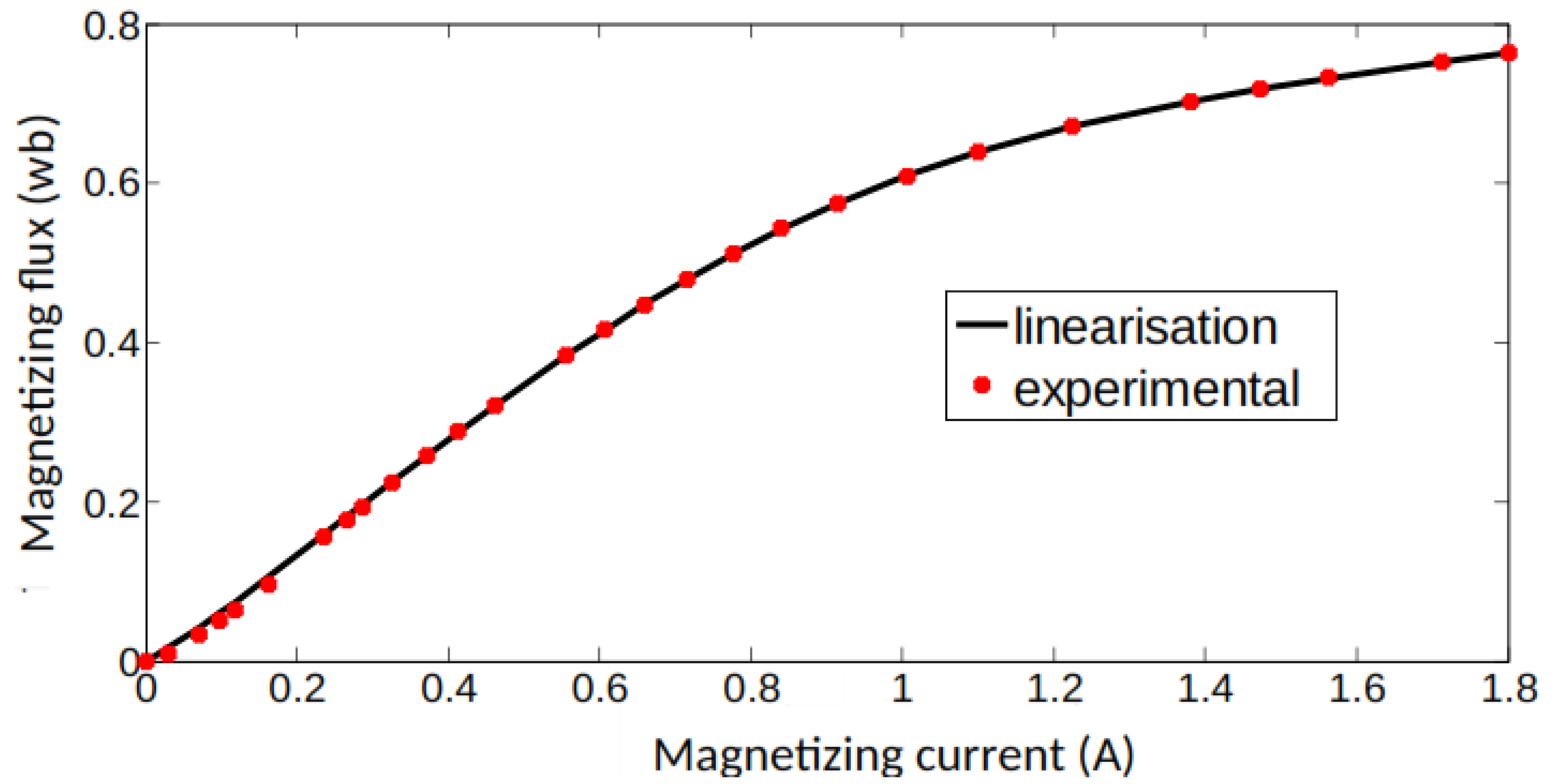
The relation ${\lambda }_m(i_m)$ is nonlinear, and this form is represented in the Figure 4.

The machine parameters are: $0.5 \mathrm{K}\mathrm{w},$ $220/380 \mathrm{V}$ $1500 \mathrm{rpm}$, $0.75 A, 50 \mathrm{Hz}, 2 \mathrm{poles},$ $R_r=14.38 \mathsf{\Omega }$ $R_s=28.59 \mathsf{\Omega }$ $X_r=19.81 \mathsf{\Omega }$ $X_{sm}=20.1 \mathsf{\Omega }$ $X_s=19.81 \mathsf{\Omega }$, and $X_s=19.81 \mathsf{\Omega }.$$R_1=R_2=1000 \mathsf{\Omega }$.

The magnetizing saturation curve of the DSIM was measured with the machine driven at synchronous speed. The estimation of the mutual-leakage effect on experimental characteristics versus magnetizing current was approximated by a polynomial of degree of 8, as follows:

$${\lambda }_m=k_1{i}_m{}^8+k_2{i}_m{}^7+k_3{i}_m{}^6+k_4{i}_m{}^5+k_5{i}_m{}^4+k_6{i}_m{}^3+k_7{i}_m{}^2+k_8{i}_m$$

(19)

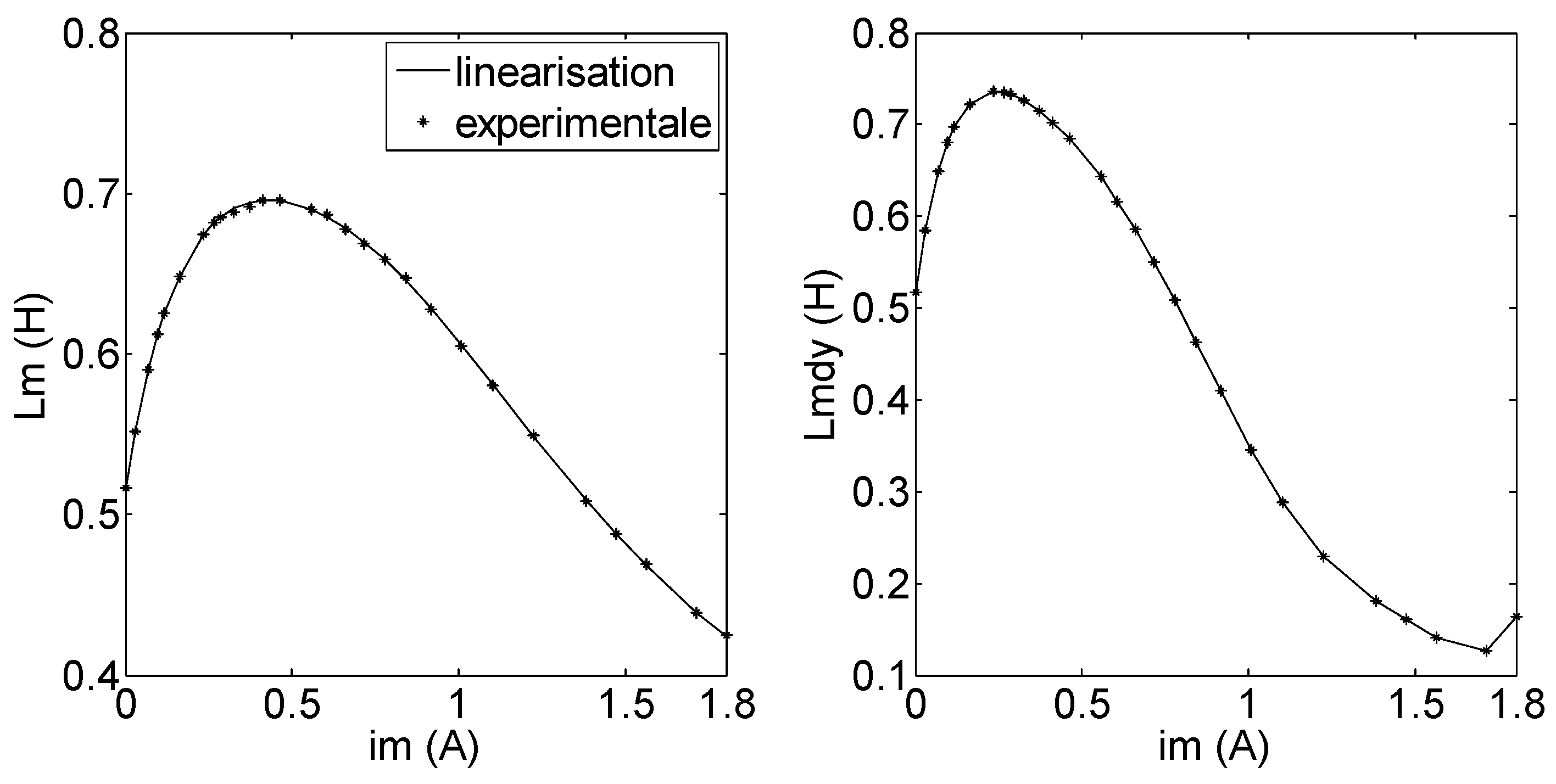
The mutual inductances, static and dynamic, are respectively defined as follows:

$$L_m=\frac{{\lambda }_m}{i_m}$$

(20)

$$L_{mdy}=\frac{d{\lambda }_m}{d{i}_m}$$

(21)

$L_m$ is the nonlinear static mutual inductance expressed by the following expression.

$$L_m=k_1{i}_m{}^7+k_2{i}_m{}^6+k_3{i}_m{}^5+k_4{i}_m{}^4+k_5{i}_m{}^3+k_6{i}_m{}^2+k_7{i}_m+k_8$$

(22)

With:

$$\begin{array}{l}{k}_1=0.19303;k_2=-1.4276;\\ k_3=4.3069;k_4=-6.8637;\\ k_5=6.4026;k_6=-3.8101;\\ k_7=1.2896;k_8=0.51665;\end{array}$$

(23)

$$L_{mdy}= 8k_1{i}_m{}^7+ 7k_2{i}_m{}^6+ 6k_3{i}_m{}^5+ 5k_4{i}_m{}^4+ 4k_5{i}_m{}^3+ 3k_6{i}_m{}^2+ 2k_7{i}_m+k_8$$

Figure 5 presents the variations in the static inductance $L_m$ and dynamic inductance $L_{mdy}$, according to the magnetizing current $i_m$. The characteristic of the static magnetizing inductance is described by a polynomial of order 7, Equation (22).

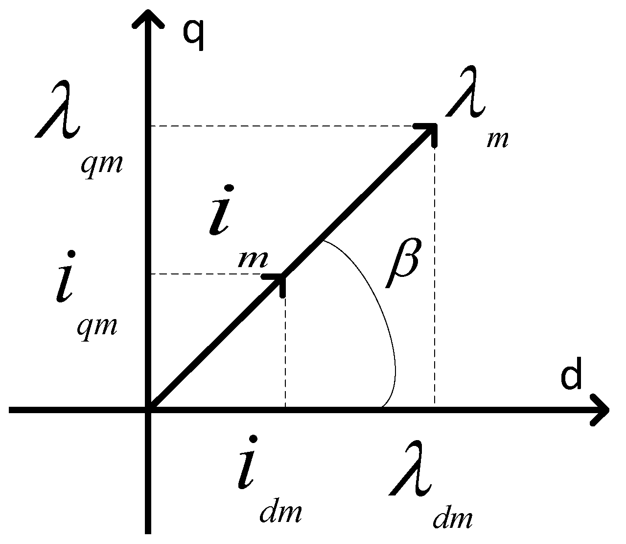
Furthermore, if we assume a sinusoidal distribution of the windings, the flux and the magnetizing current can be considered as space vectors. Since the hysteresis is neglected, these two vectors are in phase. Therefore, at a given moment, their position can be identified with respect to the axis d and chosen as a reference, using an angle $\alpha$, Figure 6.

It comes from this figure:

$$\left\{\begin{array}{l}\cos \beta =\frac{{\lambda }_{dm}}{{\lambda }_m}=\frac{i_{dm}}{i_m}\\ \sin \beta =\frac{{\lambda }_{qm}}{{\lambda }_m}=\frac{i_{qm}}{i_m}\end{array}\right.$$

With:

$$L_m\hspace{0.17em}\hspace{0.17em}=\hspace{0.17em}\hspace{0.17em}\frac{{\lambda }_m}{i_m}\hspace{0.17em}\hspace{0.17em}=\hspace{0.17em}\hspace{0.17em}\hspace{0.17em}\frac{{\lambda }_{dm}}{i_{dm}}\hspace{0.17em}\hspace{0.17em}=\hspace{0.17em}\hspace{0.17em}\hspace{0.17em}\frac{{\lambda }_{qm}}{i_{qm}}$$

Moreover, in the main system (16), it is imperative to determine the derivatives of the magnetizing, direct, and quadrature fluxes. To do this, we seek to define the formulations using the static and dynamic inductances $L_m{}_{dy}$ and $L_m$

4.1. Determination of Quantities $\frac{d{\lambda }_{dm}}{dt}$ and $\frac{d{\lambda }_{qm}}{dt}$

The leakage inductances are assumed to be constant; only the d–q magnetizing flux is subject to saturation. Deriving stator and rotor linkage fluxes leads to the time constant, with only the main flux derivative of the d–q magnetizing flux ${\lambda }_{dm},{\lambda }_{qm}$.

$$\left\{\begin{array}{l}\cos \beta =\frac{{\lambda }_{dm}}{{\lambda }_m}=\frac{i_{dm}}{i_m}\\ \sin \beta =\frac{{\lambda }_{qm}}{{\lambda }_m}=\frac{i_{qm}}{i_m}\end{array}\right.$$

(24)

Angular $\beta$ designates the position of ${\lambda }_m$ with respect to the d–q axis. It also characterizes the position of the magnetizing current $i_m$ in the air gap.

Therefore, $\frac{d{\lambda }_{dm}}{dt},\frac{d{\lambda }_{qm}}{dt}$ have to be described by means of the winding current.

$$\left\{\begin{array}{l}\frac{d{\lambda }_{dm}}{dt}\hspace{0.17em}\hspace{0.17em}=\hspace{0.17em}\hspace{0.17em}\frac{d({\lambda }_m\cos \beta )}{dt}=\hspace{0.17em}\cos \beta \frac{d{\lambda }_m}{dt}\hspace{0.17em}\hspace{0.17em}-\hspace{0.17em}\hspace{0.17em}{\lambda }_m\sin \beta \frac{d\beta }{dt}\hspace{0.17em}\hspace{0.17em}\hspace{0.17em}\hspace{0.17em}\hspace{0.17em}\hspace{0.17em}\\ \frac{d{\lambda }_{qm}}{dt}=\frac{d({\lambda }_m\sin \beta )}{dt}=\hspace{0.17em}\hspace{0.17em}\sin \beta \frac{d{\lambda }_m}{dt}\hspace{0.17em}\hspace{0.17em}+\hspace{0.17em}\hspace{0.17em}{\lambda }_m\cos \beta \frac{d\beta }{dt}\end{array}\right.$$

(25)

Terms $\cos \beta \frac{d{\lambda }_m}{dt}$ and $\sin \beta \frac{d{\lambda }_m}{dt}$ may be elaborated as follows:

$$\left\{\begin{array}{l}\cos \beta \frac{d{\lambda }_m}{dt}=L_{mdy}\frac{d{i}_{dm}}{dt}+L_{mdy}{i}_{qm}\frac{d\beta }{dt}\\ \sin \beta \frac{d{\lambda }_m}{dt}=L_{mdy}(\frac{d{i}_{qm}}{dt}-i_{qm}\frac{\cos \beta }{\sin \beta }\frac{d\alpha }{dt})\end{array}\right.$$

(26)

Therefore, (25) is written:

$$\left\{\begin{array}{l}\frac{d{\lambda }_{dm}}{dt}=L_{mdy}\frac{d{i}_{dm}}{dt}+(i_{qm}{L}_{mdy}-\sin \beta \hspace{0.17em}{\lambda }_m)\frac{d\beta }{dt}\\ \frac{d{\lambda }_{qm}}{dt}=L_{mdy}\frac{d{i}_{qm}}{dt}+({\lambda }_m\cos \beta -i_{qm}\frac{\cos \beta }{\sin \beta })\frac{d\beta }{dt}\end{array}\right.$$

(27)

$$\beta ={\tan }^{-1}(\frac{i_{qm}}{i_{dm}})$$

(28)

Thus:

$$\frac{d\beta }{dt}\hspace{0.17em}=(\frac{\cos \beta }{i_m}\frac{d{i}_{qm}}{dt}-\frac{\sin \beta }{i_m}\frac{d{i}_{dm}}{dt})$$

(29)

We can write:

$$\left\{\begin{array}{l}\frac{d{\lambda }_{dm}}{dt}=L_d\frac{d{i}_{dm}}{dt}+L_{dq}\frac{d{i}_{qm}}{dt}\\ \frac{d{\lambda }_{qm}}{dt}=L_{dq}\frac{d{i}_{dm}}{dt}+L_q\frac{d{i}_{qm}}{dt}\end{array}\right.$$

(30)

$$\left\{\begin{array}{l}{L}_d=L_m+{\cos }^2\beta (L_{mdy}-L_m)\\ L_q=L_m+{\sin }^2\beta (L_{mdy}-L_m)\\ L_{dq}=\cos \beta \sin \beta (L_{mdy}-L_m)\end{array}\right.$$

(31)

4.2. Inter-Coupling Factors

In the expressions of the derivatives of the magnetizing fluxes, one notices the appearance of additional tension terms due to the presence of the magnetic nonlinearities. Although the d–q axes are orthogonal, they appear to be magnetically coupled by means of the coefficient $L_{dq}$. If there is no saturation, $L_{mdy}$ will be equal to $L_m$, the term $L_{dq}$ will be zero, and the evoked coupling disappears. This phenomenon, related to the presence of saturation and known in the literature as cross-saturation, has been the subject of long discussions and even polemics. In conclusion, the coefficient $L_{dq}$ can be qualified as a factor of saturation and inter-coupling between the axes in quadrature.

4.3. Derivation of the Saturated Current Models

Based on the general equation of the SPIM, a mathematical model is developed to represent the dynamic characteristic involved in the voltage build-up of the SPIM. The dynamic analysis has to demonstrate the transient voltage and frequency developed by the induction generator.

After deriving the system, we can obtain the following system:

$$\left\{\begin{array}{c}\frac{d{\lambda }_{ds1}}{dt}=\left(l_s+l_{sm}\right)\frac{d{i}_{ds1}}{dt}+l_{sm}\frac{d{i}_{ds2}}{dt}+L_d\frac{d{i}_{dm}}{dt}+L_{dq}\frac{d{i}_{qm}}{dt}\hfill \\ \frac{d{\lambda }_{qs1}}{dt}=\left(l_s+l_{sm}\right)\frac{d{i}_{qs1}}{dt}+l_{sm}\frac{d{i}_{qs2}}{dt}+L_q\frac{d{i}_{qm}}{dt}+L_{dq}\frac{d{i}_{dm}}{dt}\hfill \\ \frac{d{\lambda }_{ds2}}{dt}=l_{sm}\frac{d{i}_{ds1}}{dt}+\left(l_s+l_{sm}\right)\frac{d{i}_{ds2}}{dt}+L_d\frac{d{i}_{dm}}{dt}+L_{dq}\frac{d{i}_{qm}}{dt}\hfill \\ \frac{d{\lambda }_{qs2}}{dt}=l_{sm}\frac{d{i}_{qs1}}{dt}+\left(l_s+l_{sm}\right)\frac{d{i}_{qs2}}{dt}+L_q\frac{d{i}_{qm}}{dt}+L_{dq}\frac{d{i}_{dm}}{dt}\hfill \\ \frac{d{\lambda }_{dr}}{dt}=l_r\frac{d{i}_{qr}}{dt}+L_d\frac{d{i}_{dm}}{dt}+L_{dq}\frac{d{i}_{qm}}{dt}\hfill \\ \frac{d{\lambda }_{qr}}{dt}=l_r\frac{d{i}_{qr}}{dt}+L_q\frac{d{i}_{qm}}{dt}+L_{dq}\frac{d{i}_{dm}}{dt}\hfill \end{array}\right.$$

(32)

The main differential system can be represented by:

$$\left[V\right]=\left[A\right]\left[\dot{X}\right]+\left[B\right]\left[X\right]$$

(33)

With:

$$\left[V\right]={\left[\begin{array}{cccccc}{V}_{ds1}& V_{qs1}& V_{ds2}& V_{qs2}& 0& 0\end{array}\right]}^t$$

(34)

$$\left[X\right]={\left[\begin{array}{cccccc}{i}_{ds1}& i_{qs1}& i_{ds2}& i_{qs2}& i_{dr}& i_{qr}\end{array}\right]}^t$$

(35)

$$\left[A\right]=\left[\begin{array}{cccccc}{l}_s+l_{sm}+L_d& L_{dq}& l_{sm}+L_d& L_{dq}& L_d& L_{dq}\\ L_{dq}& l_s+l_{sm}+L_q& L_{dq}& l_{sm}+L_q& L_{dq}& L_q\\ l_{sm}+L_d& L_{dq}& l_s+l_{sm}+L_d& L_{dq}& L_d& L_{dq}\\ L_{dq}& l_{sm}+L_q& L_{dq}& l_s+l_{sm}+L_q& L_{dq}& L_q\\ L_d& L_{dq}& L_d& L_{dq}& l_r+L_d& L_{dq}\\ L_{dq}& L_q& L_{dq}& L_q& L_{dq}& l_r+L_q\end{array}\right]$$

(36)

$$\left[B\right]=\left[\begin{array}{cccccc}{R}_s& 0& 0& 0& 0& 0\\ 0& R_s& 0& 0& 0& 0\\ 0& 0& R_s& 0& 0& 0\\ 0& 0& 0& R_s& 0& 0\\ 0& L_{m}w& 0& L_{m}w& R_r& (l_r+L_m)w\\ -L_{m}w& 0& -L_{m}w& 0& (l_r+L_m)w& R_r\end{array}\right]$$

(37)

The purely current model $\left({\overline{i}}_{s1},{\overline{i}}_{s2},{\overline{i}}_r\right)$, developed previously, is the heaviest to simulate. All the elements of its matrix [A] are non-zero and depend on the cross-saturation. In addition, it contains all kinds of magnetic couplings along the d-axis $(L_d)$ to the q-axis $(L_q)$ and between the d–q axes $(L_{dq})$. On the contrary, this non-advised current model is used to determine all the saturated models and any state variables.

4.4. Derivation of the Saturated Flux Models $({\overline{\lambda }}_{s1},{\overline{\lambda }}_{s2},{\overline{\lambda }}_r)$

The derivation in the flux model $({\overline{\lambda }}_{s1},{\overline{\lambda }}_{s2},{\overline{\lambda }}_r)$ requires the determination of winding currents as a function of the state variables of the model. This is made possible by combining (17) and (18) with the derivatives of (32) to form the appropriate matrices:

$$\left\{\begin{array}{c}{i}_{ds1}=\frac{1}{\sigma }\left({\lambda }_{ds1}-\frac{l_{sm}}{L_s}{\lambda }_{ds2}-\left(1-\frac{l_{sm}}{L_s}\right){\lambda }_{dm}\right)\hfill \\ i_{qs1}=\frac{1}{\sigma }\left({\lambda }_{qs1}-\frac{l_{sm}}{L_s}{\lambda }_{qs2}-\left(1-\frac{l_{sm}}{L_s}\right){\lambda }_{qm}\right)\hfill \\ i_{ds2}=\frac{1}{\sigma }\left({\lambda }_{ds2}-\frac{l_{sm}}{L_s}{\lambda }_{ds1}-\left(1-\frac{l_{sm}}{L_s}\right){\lambda }_{dm}\right)\hfill \\ i_{qs2}=\frac{1}{\sigma }\left({\lambda }_{qs2}-\frac{l_{sm}}{L_s}{\lambda }_{qs1}-\left(1-\frac{l_{sm}}{L_s}\right){\lambda }_{qm}\right)\hfill \\ i_{dr}=\frac{{\lambda }_{dr}-{\lambda }_{dm}}{l_r}\hfill \\ i_{qr}=\frac{{\lambda }_{qr}-{\lambda }_{qm}}{l_r}\hfill \end{array}\right.$$

(38)

With: $\sigma =L_s-\frac{l_{sm}^2}{L_s}$ and $L_s=l_s+l_{sm}$ The magnetizing flux equations as a function of the stator and rotor fluxes are:

$$\left\{\begin{array}{l}{\lambda }_{dm}=L_a\left({\lambda }_{ds1}\frac{l_s}{\sigma L_s}+{\lambda }_{ds2}\frac{l_s}{\sigma L_s}+{\lambda }_{dr}\frac{1}{l_r}\right)\\ {\lambda }_{qm}=L_a\left({\lambda }_{qs1}\frac{l_s}{\sigma L_s}+{\lambda }_{qs2}\frac{l_s}{\sigma L_s}+{\lambda }_{qr}\frac{1}{l_r}\right)\end{array}\right.$$

(39)

where:

$$L_a=\frac{1}{\frac{1}{L_m}+\frac{2l_s}{\sigma L_s}+\frac{1}{l_r}}$$

(40)

By integrating the previous equations, we can define the equations of the currents as a function of the state variables:

$$\left\{\begin{array}{c}{i}_{ds1}=\frac{1}{\sigma }\left(1-\frac{l_s^2{L}_a}{\sigma L_s^2}\right){\lambda }_{ds1}-\frac{1}{\sigma L_s}\left(l_{sm}+\frac{l_s{L}_a}{\sigma L_s}\right){\lambda }_{ds2}-\left(\frac{l_s{L}_a}{\sigma l_r{L}_s}\right){\lambda }_{dr}\hfill \\ i_{qs1}=\frac{1}{\sigma }\left(1-\frac{l_s^2{L}_a}{\sigma L_s^2}\right){\lambda }_{qs1}-\frac{1}{\sigma L_s}\left(l_{sm}+\frac{l_s{L}_a}{\sigma L_s}\right){\lambda }_{qs2}-\left(\frac{l_s{L}_a}{\sigma l_r{L}_s}\right){\lambda }_{qr}\hfill \\ i_{ds2}=\frac{1}{\sigma }\left(1-\frac{l_s^2{L}_a}{\sigma L_s^2}\right){\lambda }_{ds2}-\frac{1}{\sigma L_s}\left(l_{sm}+\frac{l_s{L}_a}{\sigma L_s}\right){\lambda }_{ds1}-\left(\frac{l_s{L}_a}{\sigma l_r{L}_s}\right){\lambda }_{dr}\hfill \\ i_{qs2}=\frac{1}{\sigma }\left(1-\frac{l_s^2{L}_a}{\sigma L_s^2}\right){\lambda }_{qs2}-\frac{1}{\sigma L_s}\left(l_{sm}+\frac{l_s{L}_a}{\sigma L_s}\right){\lambda }_{qs1}-\left(\frac{l_s{L}_a}{\sigma l_r{L}_s}\right){\lambda }_{qr}\hfill \\ i_{dr}=-\left(\frac{L_a{l}_s}{\sigma L_s{l}_r}\right){\lambda }_{ds1}-\left(\frac{L_a{l}_s}{\sigma L_s{l}_r}\right){\lambda }_{ds2}+\frac{1}{l_r}\left(1-\frac{L_a}{l_r}\right){\lambda }_{dr}\hfill \\ i_{qr}=-\left(\frac{L_a{l}_s}{\sigma L_s{l}_r}\right){\lambda }_{qs1}-\left(\frac{L_a{l}_s}{\sigma L_s{l}_r}\right){\lambda }_{qs2}+\frac{1}{l_r}\left(1-\frac{L_a}{l_r}\right){\lambda }_{qr}\hfill \end{array}\right.$$

(41)

By making the necessary manipulations, the matrices relating to the case $({\overline{\lambda }}_{s1},{\overline{\lambda }}_{s2},{\overline{\lambda }}_r)$ are:

$$\left[X\right]={\left[{\lambda }_{ds1}\hspace{0.17em}\hspace{0.17em}{\lambda }_{qs1}\hspace{0.17em}\hspace{0.17em}{\lambda }_{ds2}\hspace{0.17em}\hspace{0.17em}{\lambda }_{qs2}\hspace{0.17em}\hspace{0.17em}{\lambda }_{dr}\hspace{0.17em}\hspace{0.17em}{\lambda }_{qr}\right]}^t$$

(42)

$$\left[V\right]={\left[\begin{array}{cccccc}{V}_{ds1}& V_{qs1}& V_{ds2}& V_{qs2}& 0& 0\end{array}\right]}^t$$

(43)

$$\left[A\right]=\left[\begin{array}{cccccc}1& 0& 0& 0& 0& 0\\ 0& 1& 0& 0& 0& 0\\ 0& 0& 1& 0& 0& 0\\ 0& 0& 0& 1& 0& 0\\ 0& 0& 0& 0& 1& 0\\ 0& 0& 0& 0& 0& 1\end{array}\right]$$

(44)

$$\left[A\right]=\left[\begin{array}{cccccc}\hfill \frac{R_s}{\sigma }\left(1-\frac{l_s^2{L}_a}{\sigma L_s^2}\right)\hfill & \hfill 0\hfill & \hfill -\frac{R_s}{\sigma L_s}(l_{sm}+\frac{l_s{L}_a}{\sigma L_s})\hfill & \hfill 0\hfill & \hfill -\frac{R_s{l}_s{L}_a}{\sigma l_r{L}_s}\hfill & \hfill 0\hfill \\ \hfill 0\hfill & \frac{R_s}{\sigma }\left(1-\frac{l_s{l}_s{L}_a}{\sigma L_s^2}\right)& \hfill 0\hfill & \hfill -\frac{R_s}{\sigma L_s}\left(l_{sm}+\frac{l_s{L}_a}{\sigma L_s}\right)\hfill & \hfill 0\hfill & \hfill -\frac{R_{s1}{l}_{s2}{L}_a}{\sigma l_r{L}_{s2}}\hfill \\ \frac{R_s}{\sigma }\left(1-\frac{l_s^2{L}_a}{\sigma L_s^2}\right)& 0& -\frac{R_s}{\sigma L_s}\left(l_{sm}+\frac{l_s{L}_a}{\sigma L_s}\right)& 0& -\frac{R_{s2}{l}_s{L}_a}{\sigma l_r{L}_s}& 0\\ 0& -\frac{R_s}{\sigma }\left(1-\frac{l_s^2{L}_a}{\sigma L_s^2}\right)& 0& -\frac{R_s}{\sigma L_s}\left(l_{sm}+\frac{l_s{L}_a}{\sigma L_s}\right)& 0& -\frac{R_s{l}_s{L}_a}{\sigma l_r{L}_s}\\ \hfill -\frac{R_r{L}_a{l}_s}{\sigma L_s{l}_r}\hfill & \hfill 0\hfill & \hfill -\frac{R_r{L}_a{l}_s}{\sigma L_s{l}_r}\hfill & \hfill 0\hfill & \hfill \frac{R_r}{l_r}\left(1-\frac{L_a}{l_r}\right)\hfill & w_e\\ \hfill 0\hfill & \hfill -\frac{R_r{L}_{a_s}}{\sigma L_s{l}_r}\hfill & \hfill 0\hfill & \hfill -\frac{R_r{L}_a{l}_s}{\sigma L_s{l}_r}\hfill & \hfill -w_e\hfill & \hfill \frac{R_r}{l_r}\left(1-\frac{L_a}{l_r}\right)\hfill \end{array}\right]$$

(45)

5. Influence of Cross-Saturation

It was proved in the previous chapter that it is possible to model a SPIM by a multiplicity of models. The latter are obtained by simple combination of the state variables of the machine. For this purpose, the SPIM can be represented by 20 models. These models are classified into three categories: flow models, current models, and mixed models. In addition, it has been shown that, except the flux model, all the other models show a phenomenon of magnetic inter-coupling between the axes in quadrature d–q, known as cross-saturation. The model in phase currents, stator and rotor, highlights this phenomenon as clearly as possible. Thus, to study the influence of the latter on the modeling of the SPIM, it is imperative to reformulate the dynamic operating equations of the machine in terms of phase currents but while avoiding cross-saturation.

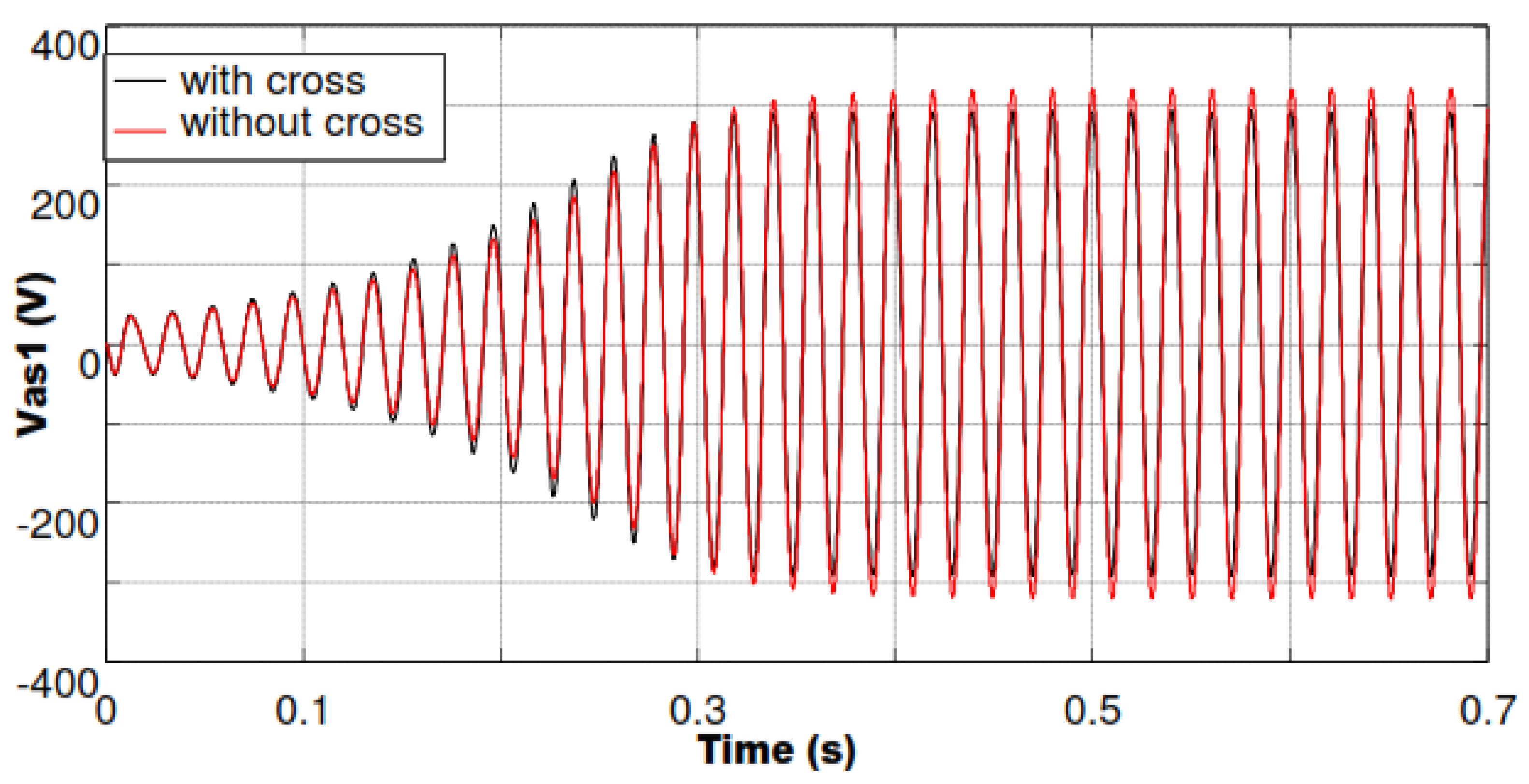
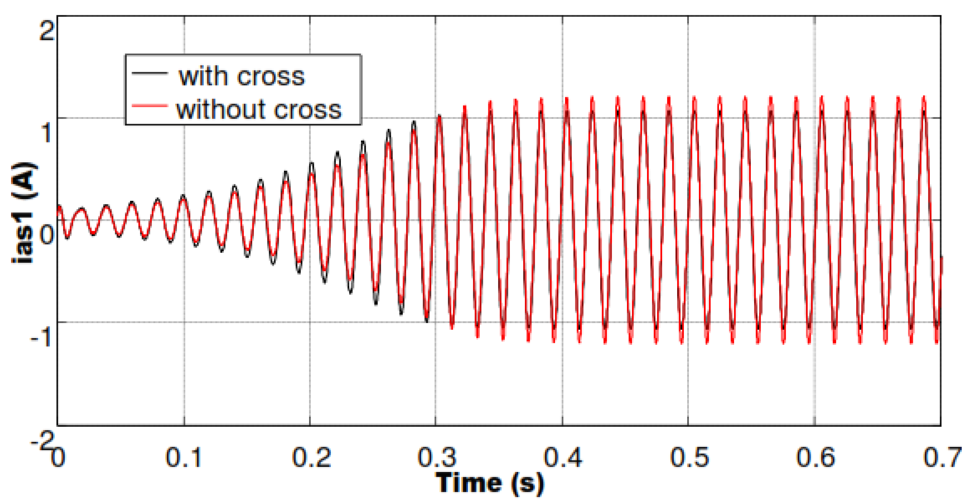
The SPIM operating in autonomous mode is very sensitive to the presence of magnetic saturation. It is a perfect application for testing the validity of models developed with and without cross-saturation. It also provides the opportunity to compare them. The following figures show the electrical and magnetic quantities at a nominal speed of N = 1500 rpm, C = 9 µF.

Figure 7 and Figure 8, respectively, describe the curves of the stator current and voltage with and without cross-saturation. In addition, they allow us to better see the difference between the two SPIM models.

The performance deviations are observed quite clearly in transient events such as voltage build-up, sudden loading, and unloading of the six-phase induction machine. The presented work shows that the full model (considering the cross-saturation effect) has faster convergence to steady-state than the one neglecting it. It is observed that the conventional model presents acceptable results, though it lacks salient details to describe the dynamic behaviour of the machine mostly when the machine is driven to the non-linear region, which is likely most of the time during specific applications. 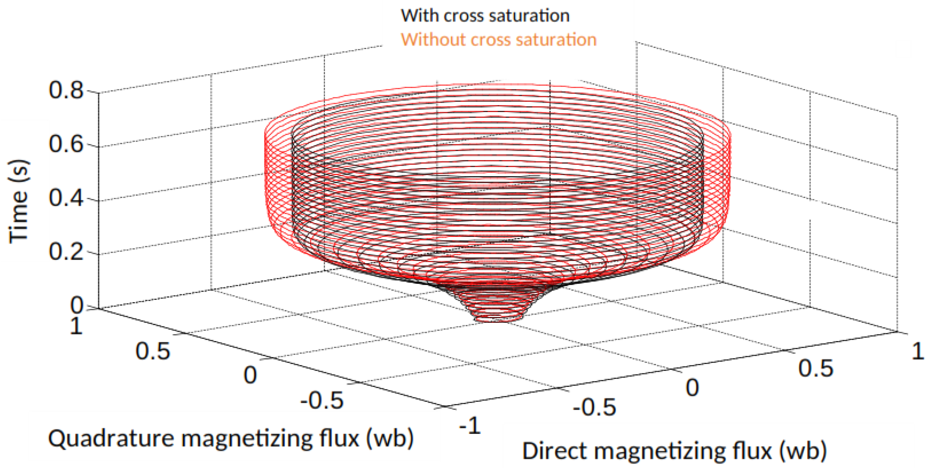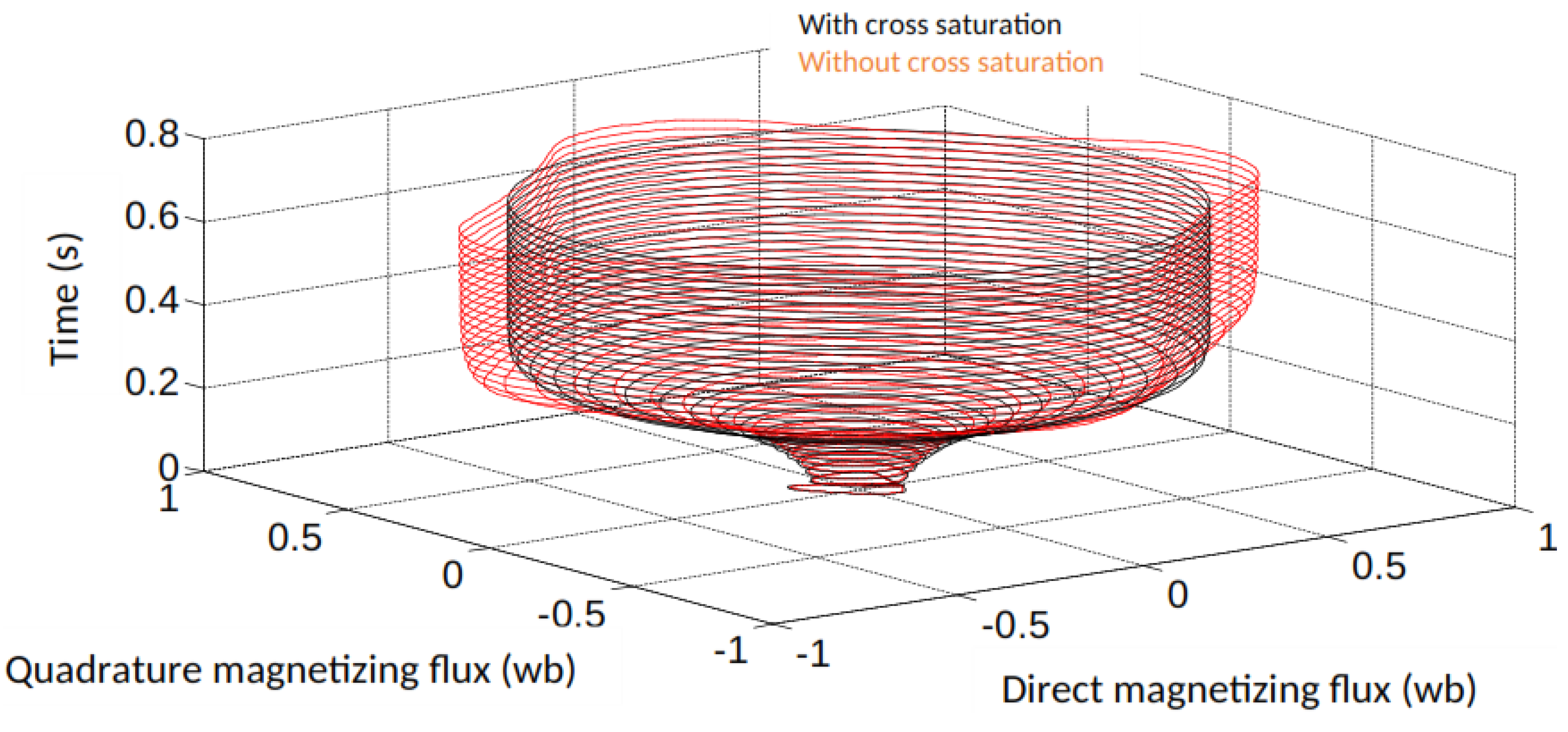Figure 9 and Figure 10 below represent the amplitudes of magnetizing fluxes and stator currents in a three-dimensional frame, with and without cross-saturation, as a function of time. The evolution of the stator current and magnetizing flux curves is established from zero and stabilizes in steady state.

The results are obtained using the phase current model $\left({\overline{i}}_{s1}, {\overline{i}}_{s2}, {\overline{i}}_r\right)$, in particular, with and without cross-saturation. Its results confirm the validity of the proposed method and the equivalence of the two models with and without cross-saturation. However, the evolutions of the different quantities as a function of time, illustrated by Figure 7, Figure 8, Figure 9 and Figure 10, prove that they do not have the same degree of sensitivity when the inter-coupling terms in the first model are ignored.

On each graph, we have shown the results obtained with the two models defined previously (full saturated model and saturated model without cross-saturation). In this current model, the matrix [A] is non-zero and depends on the magnetic saturation. Moreover, the simulation time is mainly related to the shape of the system matrix [A], the system contains null terms, and the simulation time becomes shorter. The results of the dynamic self-excitation process given in the previous figures are based on the remnant or residual flux in the iron core, providing the initial state required by the self-excitation of the SPIM. When the initial conditions of self-excitation are satisfied, the flux increases and, by associating with the growth of the magnetic fluxes, the voltage generated also increases. In the model without cross-saturation, the magnetic saturation is integrated independently along the d and q axes in the set of dynamic equations. Therefore, the model becomes simpler and faster for simulation.

The impact of cross-saturation is confirmed by the simulation time between the two models,

Table 1. Execution times of the two SPIM models with and without cross-saturation.

T (s)	Time without Cross(s)	Time without Cross(s)
0.2	22	13
0.5	56	19
0.7	72	33

, where we calculated the running time of the two models for different simulation times. The majority of its elements are null, which results in a faster simulation. Consequently, the new model, without d–q cross-saturation, is more advantageous, and its use is therefore recommended.

6. Coherence of Static and Dynamic Models

In this part, we are interested in the comparison of the results during the variations in the excitation capacity and the training speed of the self-excited SPIM between the static and dynamic regimes.

Table 2. Static and dynamic results at no load with C = 9 µF and variable speed.

Speed	Practical Values	Static Regime		Dynamic Regime
		Vas1	ΔVas1	Vas1	ΔVas1
N = 1400 tr/min	195.1	195.3	0.1%	193.74	0.69%
N = 1500 tr/min	231.2	237.6	2.69%	226.2	2.16%
N = 1600 tr/min	247.7	269.2	7.98%	239.6	3.27%

illustrates the no-load variations in the stator voltage in static and dynamic regimes for different speeds and for C = 9 µF.

From this table, it can be seen that over the speed variation range around synchronism, the rate of variation in the no-load voltage ΔV does not exceed 7.98%.

Table 3. Static and dynamic results at no load with N = 1500 rpm and variable capacity.

Speed	Practical Values	Static Regime		Dynamic Regime
		Vas1	ΔVas1	Vas1	ΔVas1
C = 7.8 µF	201.2	209.2	3.82%	197.42	1.87%
C = 8.65 µF	222.3	231.2	3.84%	216.16	2.76%
C = 9.5 µF	238.7	243.8	2.09%	230	3.64%

illustrates the no-load variations in the stator voltage in static and dynamic regimes for different values of the excitation capacity and for N = 1500 rpm.

For different values of the ignition capacity, the rate of variation in the rms voltage Vas1 between the static and dynamic regimes does not exceed 3.84%. For running under load, we consider

Table 4. Static and dynamic results under load with C = 9 µF and variable speed.

Speed	Practical Values	Static Regime		Dynamic Regime
		Vas1	ΔVas1	Vas1	ΔVas1
N = 1400 tr/min	128.7	132.6	2.94 %	125.72	2.31 %
N = 1500 tr/min	171.2	178.29	3.97 %	166.4	2.8 %
N = 1600 tr/min	177.2	182.9	3.11 %	168.2	5.07 %

and

Table 5. Static and dynamic results under load with N = 1500 rpm and variable capacity.

Speed	Practical Values	Static Regime		Dynamic Regime
		Vas1	ΔVas1	Vas1	ΔVas1
C = 7.8 µF	102.7	105	2.19 %	98	4.57 %
C = 8.6 µF	172.3	178.8	3.63 %	164.4	4.58 %
C = 9.5 µF	182.1	188.2	3.24 %	175.7	3.51 %

, which illustrate the variations in the stator voltage in static and dynamic states for different excitation capacities and speeds with R = 1000 Ω.

From the results obtained in Table 4, it is noted that the variation in SPIM drive speed under load generates a maximum stator voltage variation rate of 5.07%.

The variation in the excitation capacity for a fixed speed of 1500 rpm leads to a maximum variation rate of 4.58%. The evaluation of the static and dynamic models presented in the previous comparative tables shows that, although the static and dynamic approaches are completely different, the results are very close and present an acceptable variation rate of the stator voltage ΔV. It is concluded that the studies and modeling presented throughout this work for both static and dynamic regimes lead us to consistent results. The experimental results obtained corroborate those of the analytical study. The same approach is performed with the other two configurations, resulting in more pronounced voltage differences.

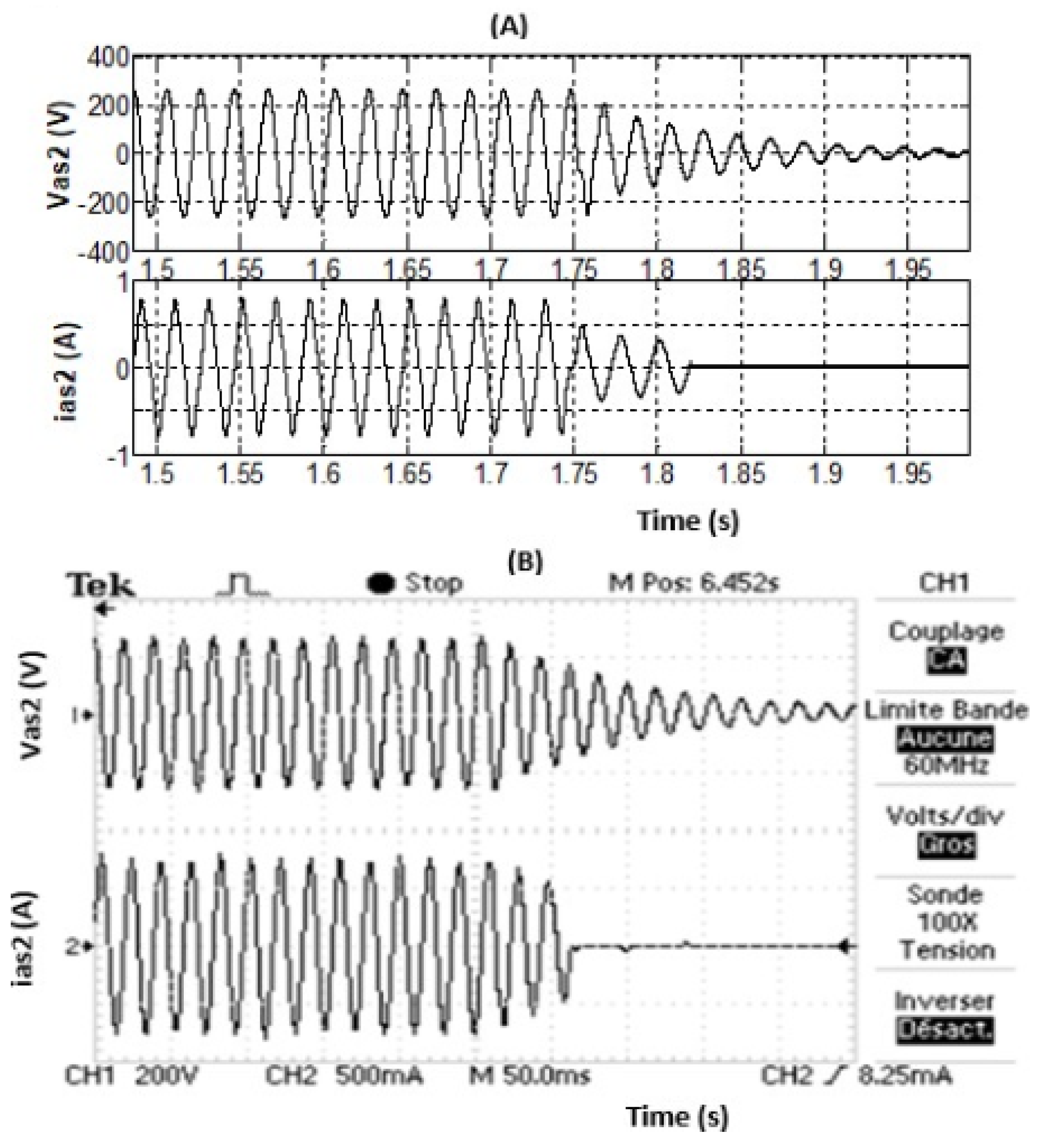
Concerning the unpriming current, when one of the three capacitors is suddenly disconnected, the self-excitation process is maintained if the value of the two remaining capacitors is sufficient to maintain the stator voltage. In the test of Figure 11, the generator is driven at 1500 rpm without load and the two values of the self-excitation capacities are fixed at 7.8 µF. At t = 1.75 s, one of the three capacitors of each star is suddenly disconnected.

The operation in an unbalanced regime obtained with the two remaining capacitors is not sufficient to maintain the self-excitation phenomenon. From the experimental test bench, we notice that the stator voltage Vas1 collapses in 0.25 s. By increasing the value of the capacitor from 7.8 µF to 9.5 µF, we note the increase in the defusing time for the voltage. Therefore, there is a risk of demagnetization of the machine.

7. Conclusions

This paper introduced an improved method based on a mathematical saturated model for six-phase induction machines based on fractional calculus. The model has been validated using a 0.5 kw prototype machine. We conducted a detailed study of the performance of the six-phase induction machine in the dynamic regime. Based on the developed mathematical developments, we simulated the models found with MATLAB. On the other hand, using the prototype present in the laboratory, we carried out practical tests to validate the theoretical study with different possible configurations of the six-phase induction machines. The experimental tests gave us encouraging results and showed us the robustness of the adopted analytical model. We considered a model without cross-saturation to compare to the already-developed model with cross-saturation. The results of the simulation as well as the experiment prove that the two models generate similar results, but the second model, without cross-saturation, is the less complicated and, therefore, recommended.

A comparison with the experimental results has demonstrated the advantages of the saturated model without cross-saturation compared to existing models. The results showed that the proposed saturated model corresponds to a closer dynamic behavior to the experimentally measured responses, especially when without cross-saturation is more pronounced.