Machine Learning for Gully Feature Extraction Based on a Pan-Sharpened Multispectral Image: Multiclass vs. Binary Approach

Abstract

Gullies reduce both the quality and quantity of productive land, posing a serious threat to sustainable agriculture, hence, food security. Machine Learning (ML) algorithms are essential tools in the identification of gullies and can assist in strategic decision-making relevant to soil conservation. Nevertheless, accurate identification of gullies is a function of the selected ML algorithms, the image and number of classes used, i.e., binary (two classes) and multiclass. We applied Linear Discriminant Analysis (LDA), Support Vector Machine (SVM), and Random Forest (RF) on a Systeme Pour l’Observation de la Terre (SPOT-7) image to extract gullies and investigated whether the multiclass (m) approach can offer better classification accuracy than the binary (b) approach. Using repeated k-fold cross-validation, we generated 36 models. Our findings revealed that, of these models, both RFb (98.70%) and SVMm (98.01%) outperformed the LDA in terms of overall accuracy (OA). However, the LDAb (99.51%) recorded the highest producer’s accuracy (PA) but had low corresponding user’s accuracy (UA) with 18.5%. The binary approach was generally better than the multiclass approach; however, on class level, the multiclass approach outperformed the binary approach in gully identification. Despite low spectral resolution, the pan-sharpened SPOT-7 product successfully identified gullies. The proposed methodology is relatively simple, but practically sound, and can be used to monitor gullies within and beyond the study region.

1. Introduction

Despite decades of focused scientific research and societal concerns [1], soil erosion by water, remains a major cause of land degradation and increasingly threatens agriculture in both developed and developing nations [2]. Globally, approximately 12 million hectares of productive land are lost due to soil erosion [1,3]. Urgent intervention is required to prevent not only further damages to productive land but also prevent irreversible loss of ecosystem services [3,4]. Soil erosion results from natural factors but anthropogenic activities including unsustainable land use practices are thought to accelerate soil erosion [2,5,6,7,8]. Soil erosion by water can manifest itself in manifolds, i.e., sheet, rill, and gully erosion [9]. Gully erosion is the most detrimental of all forms of erosion because it can quickly remove and transport enormous quantities of soil [10]. Globally, it is reported that gullies contribute around 50%–80% of total sediment production in semiarid regions [11]. Gullies can damage infrastructure such as roads and buildings [12,13]. South Africa, a semiarid country, is among severely eroded countries in Africa, with over 70% of its land subject to erosion of varying intensities [14]. Soil erosion has wide reaching implications for South Africa from both the environmental and socio-economic standpoints. Hoffman and Ashwell [15] reported that South Africa incurs about $836 million USD a year on erosion-related costs, including off-site costs for purification of silted dam water. Soil erosion, especially gullies, pose a serious threat to subsistence agriculture in most rural parts of South Africa [16,17].

Remote sensing, defined as the science or practice of acquiring data about the earth’s surface features from a distance [18,19], is not only cost-effective and quick compared to traditional field measurements, but more importantly, the data acquired through remote sensing is readily available in digital format [20]. From the aspect of accessibility, the benefits of using remote sensing technology in gully erosion mapping, especially in remote locations, cannot be stressed enough. Studies using remote sensing have grown rapidly over the past few years [21,22,23,24,25,26], following the improvement in computer processing power coupled with increased availability of free remotely sensed data such as ASTER, Landsat and Sentinel. However, the coarser spatial resolution of these sensors usually inhibits their ability to automatically detect individual gullies with sufficient detail [27]. Even at regional scales, some previous attempts to automatically classify erosion from low resolution sensors generally yielded low accuracies [26]. High spatial resolution sensors like WorldView or GeoEye can be appropriate to identify gullies, but their relatively high acquisition costs can limit the possible users. However, there can be a trade-off between accuracy and cost, and a decision as to which sensor to use is contingent upon the objectives of the study along with the availability of financial resources. Apparently, low-cost sensors such as the Systeme Pour l’Observation de la Terre (SPOT) data may be a reasonable compromise between acquisition costs and sensor accuracy, at least in the context of developing countries, particularly South Africa, where SPOT data are obtainable at substantially low costs and even free of charge.

Like sensor selection, the selection of a suitable image classification method is as much important. Deep Learning (DL) has recently become of interest in remote sensing community [28,29,30]. Some of the advantages of DL over conventional Machine Learning (ML) algorithms include high level of automation, adaptability to new challenges in the future, and can solve highly complex problems [31]. Despite its great potential, a major drawback with DL is that it requires huge amounts of data to perform well and is computationally expensive to train [32,33,34]. Consequently, ML algorithms such as Decision Tree (DT), Random Forest (RF), Support Vector Machines (SVM), Artificial Neural Network (ANN), and Discriminant Analysis (DA) are still widely used [35,36,37]. Owing to their relatively high speed and accuracy, together with the ability to accommodate non-linearity and multicollinearity [10,38,39], ML methods have become popular in soil erosion studies over the past few years [25,40,41,42,43]. Among these ML methods, SVM and RF consistently showed better performance relative to other ML methods [44], but when compared among themselves (SVM and RF), it is still unclear which method can outperform the other. Usually, the results vary from one study area to another [41]. This variation, for the most part, can be attributed to the fact that gully erosion is a complex phenomenon, which varies greatly spatially, spectrally and even temporally across different study regions [45]. Although the SVM and RF methods have been widely used, attempts to evaluate their performance in gully feature extraction in two or more spatially independent study areas (with one area used as training and another as testing) are rare. This approach eliminates the potential for overfitting, a serious problem associated with powerful classifiers like ML-based methods, where the classifier maps the training data so precisely that it is not able to generalize well [46]. Herein, we trained the models on one study area and tested them with repeated cross-validation on two other spatially independent areas, which can ensure reliable outcome measures supporting better generalization of these classifications. Whereas this approach was recently used in sinkhole feature extraction [47] and in gully feature extraction [48], the application of the SVM and RF methods were not reported. Nevertheless, these studies provide the impetus for testing the performance of these ML methods, including the Linear Discriminant Analysis (LDA), another promising ML method.

In this study, the selected ML methods are applied to a newly launched SPOT-7 multispectral (pan-sharpened) product whose potential in gully feature extraction has not been tested before until now. Besides, so far, there has not been any direct attempt to evaluate the impact of the class number on the classification accuracy of gully erosion. Yet, the class number is among major factors affecting image classification, thus, the resulting accuracy [49]. We proposed a simple, but practically relevant methodology consisting of three ML algorithms (RF, SVM, LDA) × two approaches of class numbers (binary and multiclass) × six combinations of study areas as train and test sets. The primary objective of this study was to evaluate the accuracy of the LDA, SVM, and RF methods in gully feature extraction across three spatially independent study areas. Our hypotheses were the following: (i) SPOT-7 pan-sharpened product can offer acceptable classification accuracy of gully erosion, (ii) application of multiclass approach can results in better classification accuracy in relation to the binary (eroded and non-eroded) approach.

2. Materials and Methods

2.1. Study Area

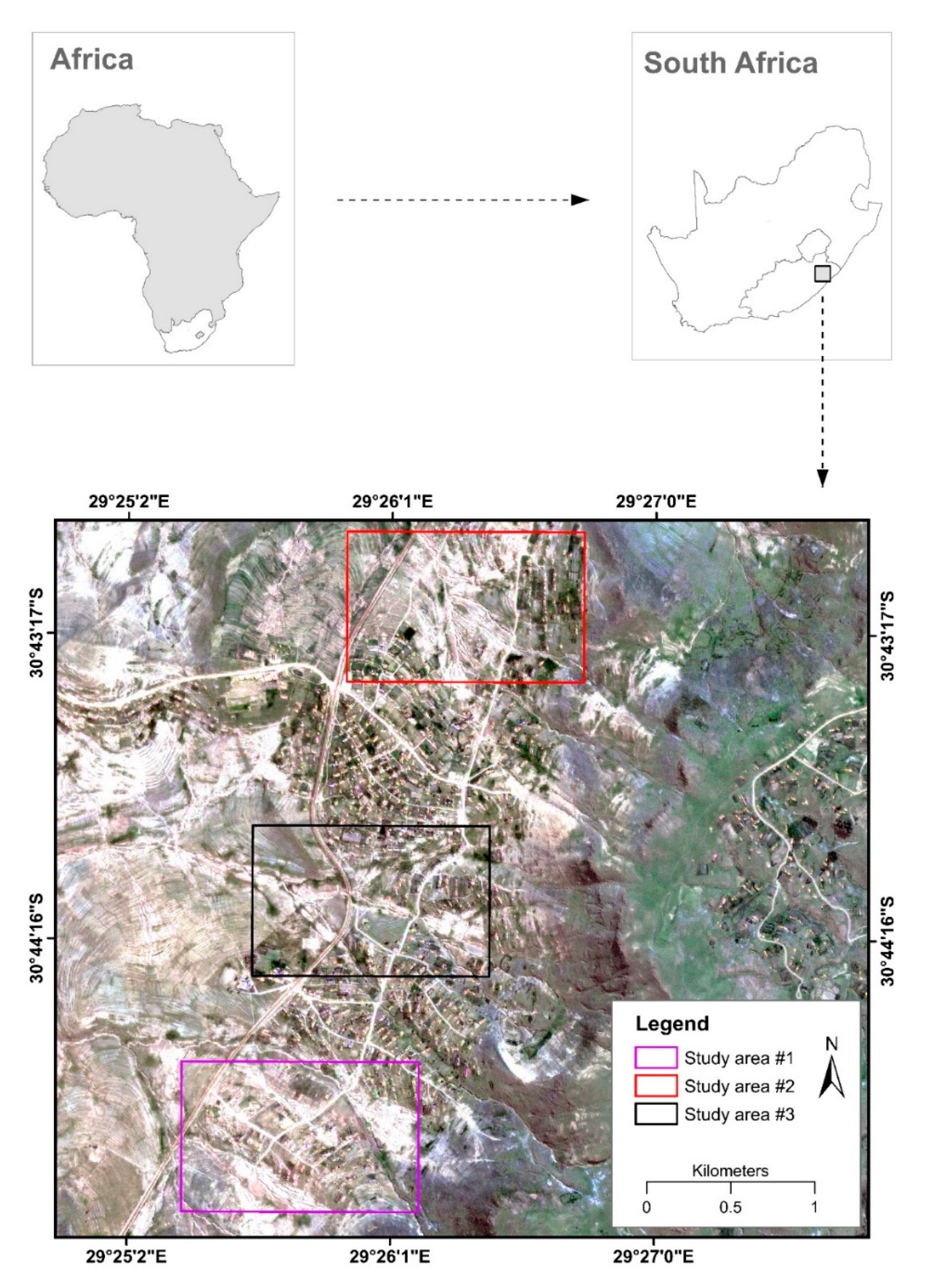
Our area of investigation is located in the Eastern Cape Province, South Africa, and consists of three study areas (s1–s3), each covering 1.26 km² (Figure 1). Extensive erosion features, mainly gullies, commonly occur in relatively gentle slopes whereas rills are found in steep sloping areas. The area has a mixture of land use types including the built-up areas characterized by dispersed rural settlements, unpaved road networks, and agricultural activities. Agriculture, including crop and animal farming, is common in the region. The climate is semiarid: winter is frequently dry and cold followed by occasionally intense rainfalls in summer. The average annual rainfall is 671 mm with yearly temperatures varying from 7 to 30 °C. Topography is highly uneven across the region. It ranges from approximately 1098 m in the central parts to more than 1500 m in the hilly northern and eastern parts of the study area. The vegetation is predominantly grassland, distributed across the elevated and mountainous areas. Low-lying areas with gentle slope, where most human activities like settlement and farming take place, have sparse vegetation cover.

2.2. Data Acquisition and Pre-Processing

The data used in this study consist of the SPOT-7 image, obtained from the South African National Space Agency (SANSA). In South Africa, SPOT-7 image is available at no cost for educational purposes or PhD research, in our case, and/or research projects that are of public interest to the country. The image contains four multispectral bands: red, green, blue (altogether RGB), and near infrared (NIR) with 5.5 m geometric resolution and a high-resolution panchromatic band (1.5 m). We improved the low geometric resolution of the SPOT-7 multispectral image using the panchromatic band from the same sensor. The Gram–Schmidt pan-sharpening method was applied, which is a widely used and accepted image fusion technique for images obtained from the same sensor [50,51,52]. ENVI software was used for pan sharpening (ENVI version 5.3—Exelis Visual Information Solutions, Boulder, Colorado).

2.3. Gully Feature Extraction from Satellite Image

In order to extract gully features, we employed three ML methods: RF, SVM, and DA. Being the most widely used ML methods, the selected ML methods have been embedded in various software packages [53]. In this study, we ran all three ML methods in Python programming environment.

2.3.1. Random Forest (RF)

RF is a robust non-parametric classifier, which is independent of assumptions on data distributions or homoscedasticity. The algorithm uses several hundred of decision trees with bagging [54]. All trees have a unique set of cases resampled from the train dataset. Sampling is performed by random selection and bootstrapping with replacements drawn from original observations, i.e., the same case can have multiple appearance in the realizations [55]. Furthermore, the number of variables involved for decision trees is the square root of the total number of variables. Each decision tree contributes a single vote to the classification, and the class with the majority vote is selected as the final classification outcome [44,56]. The larger the number of variables, the more diverse the trees become. According to variable sampling, the algorithm determines variable importance, that is, if an omitted variable results in large decrease in average accuracy, it will be considered important. RF is considered to be accurate and was successfully applied for several tasks including but not limited to grassland species discrimination [57], invasive species identification [58], soil erosion mapping [56,59,60], soil organic carbon stock mapping [61], tree species classification [62], and extracting water-related features [63]. We employed the RF model to extract gully erosion features. In the RF model, we set the ntree (number of tress) parameter to 100 and the Gini impurity was selected as the split criterion. The mtry (number of features in each split) parameter was left at its default value (i.e., mtry = 2).

2.3.2. Support Vector Machines (SVM)

Proposed by Vapnik [64], the SVM model is based on statistical learning theory to overcome problems relating to regression and classification [65,66,67]. Since its introduction, the model has been in widespread use in several researches [35,44,56,68]. The model searches for the right boundary surface among data points belonging to different classes. The aim is to find a flat boundary, called hyperplane, which can separate the classes into homogeneous partitions where each partition contains only data points of a given class. The model works well only with linear data space, and in cases of complex and higher dimensional space, the so-called ‘kernel-trick’ is used to transform the non-linear data to linear where hyperplanes can be applied [69]. SVM has two important parameters. (i) The C parameter penalizes the misclassifications: a low C value results in a simple model with soft margin, while a model with large C value prioritizes the perfect classifications; and (ii) the γ parameter defines the role of a single training pixel: too small values result in constrained models, whereas too large values lead to overfitting, and both small and large γ-values can perform poorly with a test dataset [70]. Several common kernel functions for the SVM model include linear, Radial Basis Function (RBF), polynomial, and sigmoid [49]. In the current study, we applied the SVM model with the RBF kernel function.

2.3.3. Linear Discriminant Analysis (LDA)

Discriminant Analysis (DA) is a parametric classification method requiring multivariate normal distribution, equal covariance matrices and prefers equal number of cases within categories [71]. In this study, we applied a linear DA (LDA), an ordination technique, i.e., dimension reduction, which substitutes the original variables (bands) with discriminant functions (DFs). DF scores are calculated in the m dimensional space defined by the input variables (where m is the number of a priori categories), in our case it meant land cover types, based on decision boundaries, which can either be of linear or quadratic functions [51,72]. LDA had been successfully applied in land degradation [73]. We applied linear functions for the classification of gullies.

2.4. Reference Data Collection and Accuracy Assessment

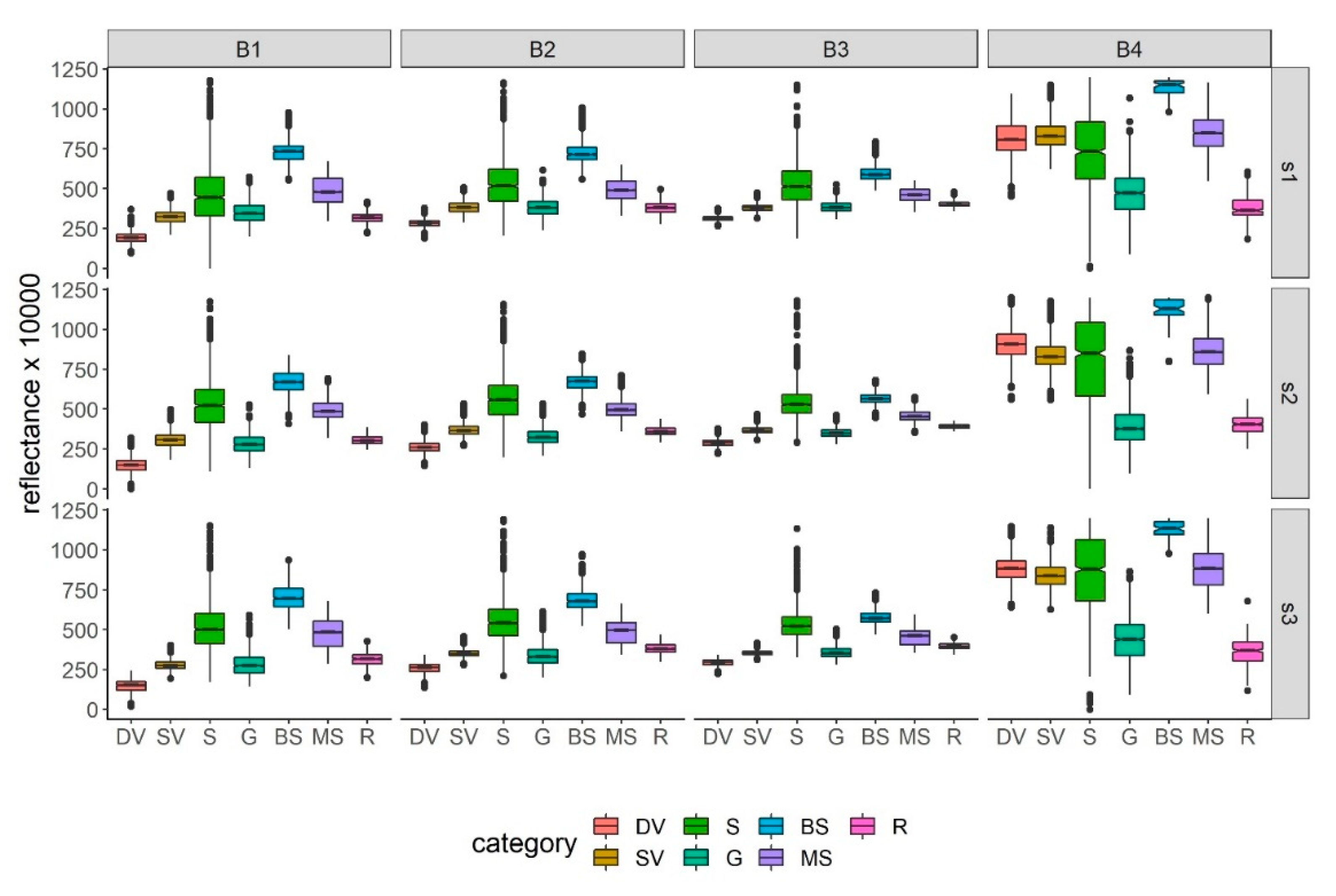
We collected the reference data based on a field survey, high-resolution SPOT image, and ancillary data (Google Earth). The reference data is not publicly available but can be provided to anybody on request. We delineated those areas where the land cover were identifiable both in the field and in the images; therefore, seven land cover classes had been distinguished: dense vegetation (DV), stressed vegetation (SV), gully (G), bare soil (BS), mixed bare soil (MS), i.e., exposed rocks, unpaved roads, bare soils, etc., settlement (S), and the roads (R). Besides, we intended to reveal the case when land cover was classified only into two classes: gully and non-gully areas; thus, as another approach we investigated the case when all non-gully classes were reclassified into one class. In the following, we refer to the seven-class solution as ‘multi-class’ (m), and the two-class solution as ‘binary’ (b) approach.

We evaluated the classification accuracy of the algorithms with repeated 10-fold cross-validation using three repetitions. We applied stratified random sampling of the whole data sets (20,795, 31,784, and 22,512 data, respectively, in s1, s2, and s3 areas): we selected 1000–1000 cases for the binary approach and 350 cases per category for the multiclass approach from the whole reference dataset, depending on the available number of data per classes and to avoid autocorrelation (selecting adjacent pixels). This approach did not require a train and test database, as the whole dataset was randomly split into 10 subsamples and 9 were used to train the models and 1 for testing and the procedure ends when all subsamples were used as a test set against all the other subsamples [74,75]. Finally, it was repeated three times and accuracy measures of 30 models can be used to evaluate the models’ performance with median and quartiles.

Although cross-validation is a reliable tool, it does not provide information on the class level accuracies; thus, we also used the confusion matrix. This matrix provides class-specific accuracies like Producer’s Accuracy (PA) and User’s Accuracy (UA), which indicate commission and omission errors, respectively [18,19,76]. PA is the probability that a pixel of a given class was classified correctly whereas UA is the probability that a given pixel was predicted to be in the class it was supposed to be [77,78,79].

Table 1. Accuracy assessment indices [79].

Accuracy	Equation	Description
Producer’s accuracy (PA)	$\mathrm{PA}=\frac{{\mathrm{n}}_{\mathrm{ii}}}{{\mathrm{n}}_{\mathrm{icol}}}$	Where ${\mathrm{n}}_{\mathrm{ii}}$ is the number of pixels correctly classified in each class; and ${\mathrm{n}}_{\mathrm{icol}}$ is the column total representing reference data.
User’s Accuracy (UA)	$\mathrm{UA}=\frac{{\mathrm{n}}_{\mathrm{ii}}}{{\mathrm{n}}_{\mathrm{irow}}}$	Where ${\mathrm{n}}_{\mathrm{irow}}$ is the row total representing predicted classes.
Overall Accuracy (OA)	$\mathrm{OA}=\frac{1}{\mathrm{N}}{\displaystyle \sum _{\mathrm{i}=1}^{\mathrm{r}}}{\mathrm{n}}_{\mathrm{ii}}$	Where N is the total number of pixels in the confusion matrix, and r is the number of rows.

provides basic information on the calculation of the accuracy indices used.

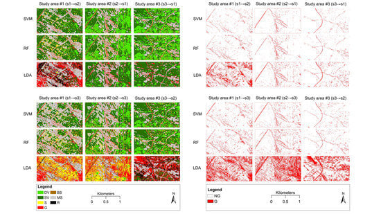
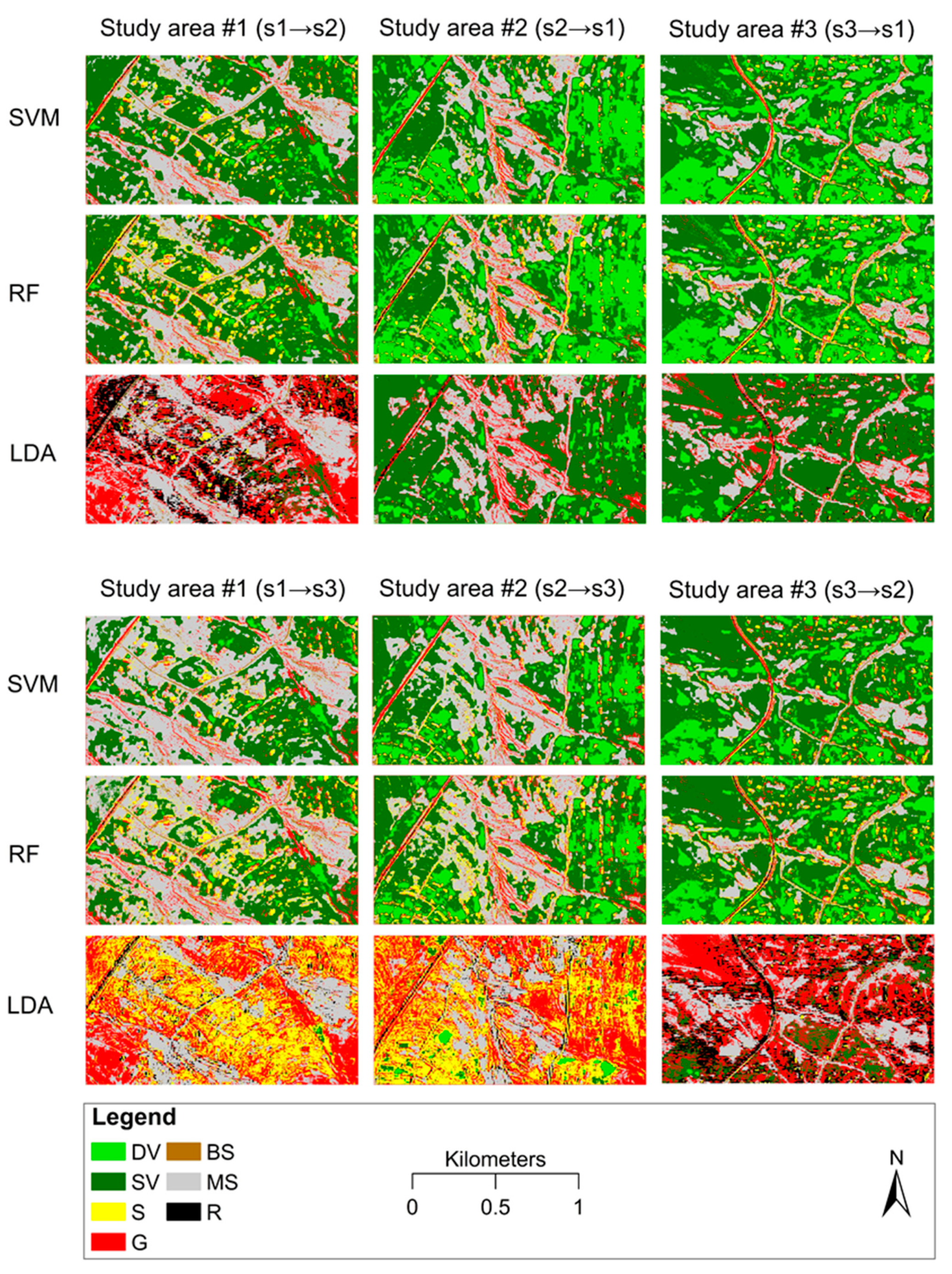
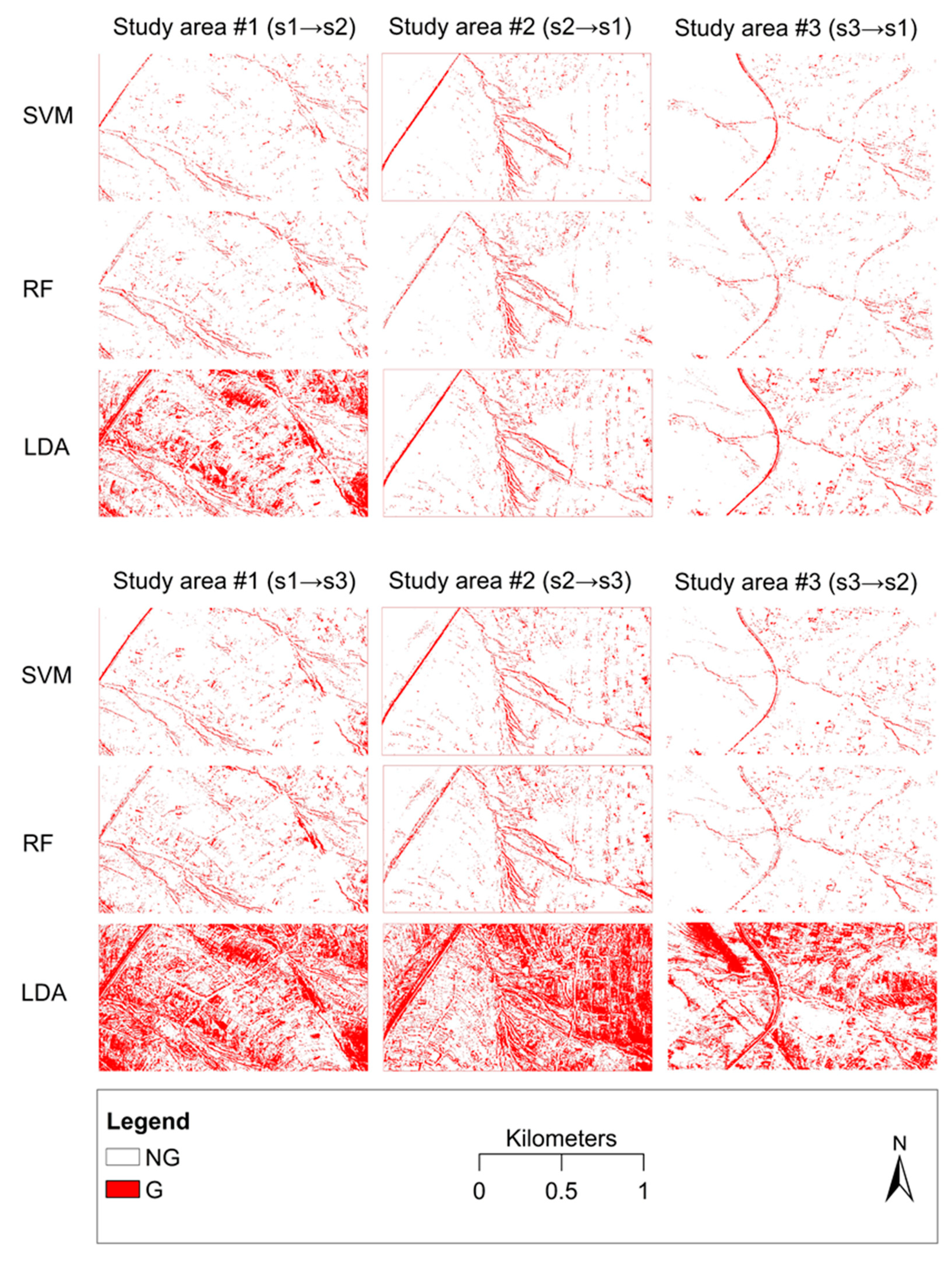
Overall Accuracy (OA), which is a ratio of correctly classified pixels, was also calculated, but on the usual way: we had three study areas (s1-s3), and one was used to train the model and another to test it. In other words, train data of one study area (e.g., s1) was used to perform the model generation and this model was applied on completely independent data of the other two study areas (s2 and s3). We repeated this procedure in all combinations of the study areas; thus, altogether we had 36 models: 3 ML algorithms (RF, SVM, LDA) × 2 approaches of class numbers (binary and multiclass) × 6 combinations of study areas as train and test sets (s1→s2, s2→s1, s2→s3, s3→s2, s1→s3, s3→s1).

2.5. Statistical Evaluation

Shapiro–Wilk test was used to check the assumption of normal distribution [80]. Reference data of the land cover classes were skewed, but classification accuracy measures (UA, PA, OA) followed the normal distribution. We applied hypothesis testing to explore if the land cover classes had the same medians (H0) or differed from each other (H1); i.e., we evaluated the training datasets from the aspect of differences in reflectance. For example, if reflectance values differ, we can suppose that classification of the satellite image can successfully distinguish gullies from other land cover classes. In case of the binary approach, we applied the Yuen test with 0.2 value of trim and 599 times bootstrapping [81], while for multiclass approach, robust ANOVA was used with a post hoc test based on trimmed means (using the WRS2 package of R). For Yuen test, we also evaluated the effect size (ξ), which is a standardized measure to quantify the magnitude of difference; therefore, it can be compared with the analysis performed on different datasets. Calculation of effect sizes for the multiclass approach is not defined for robust ANOVA. Therefore, we applied the Dunnett’s test [82], using gullies as a control and all other land cover classes were compared with it. This way, we were able to calculate the confidence intervals of differences instead of effect sizes, but we were also able to see how the differences were distributed around zero. At the same time, we limited the number of comparisons and the degree of freedom (avoiding a full factorial comparison). Besides, considering the aim of this study, which was to extract gullies, this was a reasonable step.

Model performance conducted on classification accuracy measures was evaluated with General Linear Modelling (GLM) using the study areas, the number of classes (i.e., binary or multiclass) and the algorithms as factors in different combinations and the UA and PA as dependent variables. In this case, we applied the ω² as a measure of effect size, which is less biased by the low sample size (in our case, it was limited to the results of 36 models), as suggested by Levine [83]. Statistical analyses were performed in R 3.6.2 software [84], with the WRS2 [85], jamovi 1.2. [86], and with the GAMLj module [87].

3. Results

3.1. Differences in Reflectance Values

Results confirmed that, generally, all bands had significantly different values in case of the binary approach; the only exception was observed in case of the blue band, in Study area #1 (Figure 2). However, effect sizes indicated only small effect for red and blue bands, medium for green and large for NIR (

Table 2. Results of robust independent samples t-test performed on SPOT-7 bands using the binary (gully—non-gully) approach (study areas: s1–s3, t: value of t-statistic, p: significance, ξ: effect size).

Bands	s1			s2			s3
	t	p	ξ	t	p	ξ	t	p	ξ
Red	8.3	<0.001	0.159	9.55	<0.001	0.14	6.74	<0.001	0.11
Green	2.99	0.003	0.062	28.21	<0.001	0.38	15.98	<0.001	0.28
Blue	1.07	0.286	0.02	14.42	<0.001	0.2	9.56	<0.001	0.17
NIR	86.1	<0.001	0.964	171.7	<0.001	0.98	113.3	<0.001	0.98

). Therefore, NIR band had the largest relevance in discriminating the gullies. Next, we repeated the analysis with the multiclass approach (Figure 3), using seven categories, and the robust ANOVA test confirmed significant models for each combination of bands and study areas (

Table 3. Results of robust ANOVA performed on SPOT-7 bands using the multiclass (7-classes) approach (study areas: s1–s3, F: value of F-statistic, p: significance).

Bands	s1		s2		s3
	F	p	F	p	F	p
Red	10105	<0.001	25193	<0.001	12660	<0.001
Green	9309	<0.001	21188	<0.001	10571	<0.001
Blue	9718	<0.001	25694	<0.001	13036	<0.001
NIR	3590	<0.001	10905	<0.001	4317	<0.001

).

As ANOVA only reports that there is at least one significantly different category, a post hoc test was needed to reveal the differences among the categories. With seven categories, there are too many combinations with pairwise comparison; therefore, we focused only on the difference in gully and the other categories, according to the primary aim of this study. Gullies usually had significant differences, but mostly in red and green bands, differences were not of significant with the stressed vegetation and the roads (Table 3). In this case, we presented the mean differences of the land cover categories. Confidence intervals were in accordance with the post hoc test, except in the study area #2 (s2) where the robust post hoc test indicated significant differences (

Table 4. Results of robust ANOVA performed on SPOT-7 bands using the multiclass (7-classes) approach (LC: land cover, study areas: s1–s3, G: gully, DV: dense vegetation, SV: stressed vegetation, S: settlement, BS: bare soil, MS: mixed soil, R: road).

LC	s1				s2				s3
	Red	Green	Blue	NIR	Red	Green	Blue	NIR	Red	Green	Blue	NIR
G-DV	<0.001	<0.001	<0.001	<0.001	<0.001	<0.001	<0.001	<0.001	<0.001	<0.001	<0.001	<0.001
G-SV	<0.001	0.275	<0.001	<0.001	<0.001	<0.001	<0.001	<0.001	0.281	0.275	0.883	<0.001
G-S	<0.001	<0.001	<0.001	<0.001	<0.001	<0.001	<0.001	<0.001	<0.001	<0.001	<0.001	<0.001
G-BS	<0.001	<0.001	<0.001	<0.001	<0.001	<0.001	<0.001	<0.001	<0.001	<0.001	<0.001	<0.001
G-MS	<0.001	<0.001	<0.001	<0.001	<0.001	<0.001	<0.001	<0.001	<0.001	<0.001	<0.001	<0.001
G-R	<0.001	0.528	<0.001	<0.001	0.614	<0.001	<0.001	<0.001	<0.001	<0.001	<0.001	<0.001

), while the confidence intervals (Figure 4, based on Dunnett’s test statistics) showed non-significance between gullies and roads.

3.2. Gully Feature Extraction

Gully classification results based on the multiclass and binary approach are presented in Figure 5 and Figure 6, respectively. SVM and RF showed more or less the same results, whereas LDA yielded completely different results, most notably in study area #1 (s1→s2, s1→s3), study area #2 (s2→s3), and study area #3 (s3→s2). However, in some cases, i.e., study area #2 (s2→s1) and study area #3 (s3→s1), LDA showed almost the same results as SVM and RF. Overall, the multiclass and binary approach appear to have yielded almost the same results in terms of gully extraction, although there are slight differences in accuracy results, as presented in the sub-sections that follow (Section 3.3 and Section 3.4).

3.3. Overall Model Performance Evaluation

Overall accuracies, based on three times, repeated 10-fold cross-validation (i.e., results of 30 models), showed that gully identification can be successful if we use RF or SVM classification algorithms. Both RF and SVM provided similar accuracies; medians were between 92%–96%. Binary approach resulted in better OA values; nevertheless, the multiclass (m) classification was only 2% worse than the binary (b) (Figure 7). The rank was the same in all study areas in the first three places: SVMb, RFb, LDAb with the binary approach, then the multiclass classifications had some mixing on the 4th place between SVMm and RFm, but LDAm always had the worst performance. Regarding the first two places, SVMb had only a slight superiority (<0.5%) and, additionally, lower quartiles were higher for RFb; thus, generally, these models can be regarded as more reliable. Furthermore, the multiclass approach was not as effective as the binary approach, even the LDAb’s lower quartiles were higher in all study areas than the best multiclass solution’s upper quartile, and differences were 2%–8%.

3.4. Model Performance Evaluation on Class Level

Class level evaluation was performed only with the accuracy metrics of gullies. Results showed that most classifiers failed to produce both high PA and UA values (Figure 8). Worst performances belonged to the LDA algorithm, UA values of the multiclass classification was under 30%, misclassifications meant large number of commission error, large number of pixels were classified as gullies, which belonged to other categories; although, we also have to note that there were also successful models (L-m-2-1 was as good as some RF and SVM models). Regarding the best 80–80% quarter (Figure 8), there were 4 RF and 3 SVM models, 2 binary and 5 multiclass types. In this quarter, where the errors were within a reasonable measure, highest UAs belonged to R-b-2-3 (86.0%) and R-m-2-3 (83.8%), while PAs were 95.1% and 96.1%, respectively. Nevertheless, highest PA belonged to the R-b-3-2 (93.7%) but the corresponding UA was only 79.4%. Best PA belonged to an LDA model (L-b-2-3) with 99.5% but its UA was only 18.5%.

3.5. Statistical Evaluation of Factors Biasing Class Level Performance

GLM revealed that study areas and the algorithms can provide explanations for the different efficiency of the classification models; adjusted R²s indicated 59.3% explained variance for UA and 56.1% for PA (

Table 5. Summary of General Linear Modelling (GLM) performed with PA as independent variable (Alg: algorithm, type: binary or multiclass approach, stud: Study area; SS: Sum of Squares, df: degree of freedom, F: F-statistic, p: significance, ω²: effect size; p < 0.05 is highlighted with bold).

Source	SS	df	F	p	ω²
Model	3200.5	17	3.632	0.005	0.554
Alg	174.9	2	1.687	0.213	0.017
type	25.5	1	0.493	0.492	0.006
stud	1431.9	2	13.811	<0.001	0.317
Alg × type	946.7	2	9.132	0.002	0.201
Alg × stud	323	4	1.558	0.228	0.028
type × stud	99.1	2	0.956	0.403	0.001
Alg × type × stud	199.4	4	0.962	0.452	0.002
Residuals	933.1	18
Total	4133.6	35

and

Table 6. Summary of GLM performed with UA as independent variable (Alg: algorithm, type: binary or multiclass approach, stud: Study area; SS: Sum of Squares, df: degree of freedom, F: F-statistic, p: significance, ω2: effect size; p < 0.05 is highlighted with bold).

Source	SS	df	F	p	ω²
Model	20,720.3	17	4.0014	0.003	0.586
Alg	17,390.9	2	28.547	<0.001	0.633
type	82.6	1	0.2711	0.609	0.008
stud	2413.4	2	3.9615	0.038	0.068
Alg × type	98.6	2	0.1618	0.852	0.019
Alg × stud	666.8	4	0.5473	0.703	0.021
type × stud	18.7	2	0.0307	0.97	0.022
Alg × type × stud	49.4	4	0.0405	0.997	0.044
Residuals	5482.8	18
Total	26203.1	35

). Study area had significant effect on both the PA and UA results, but the applied algorithm had significant direct effect only on PA.

In case of PA, the interaction between the algorithms and study areas was not significant. Effect size (ω²) indicated large effect for the study areas for PA, and for the algorithms for UA. Furthermore, the interaction was significant between the applied algorithms and the type (number of categories), i.e., classification algorithms perform differently with the binary or multiclass approaches.

4. Discussion

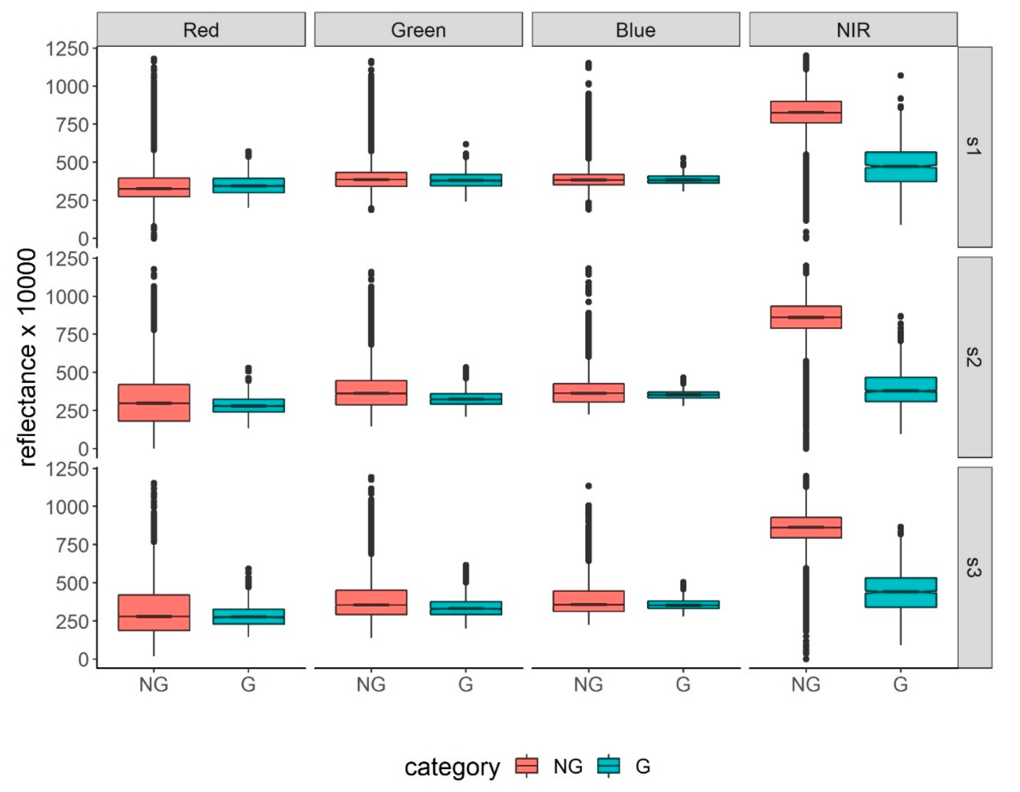
Despite the spectral heterogeneity of gullies, spectral differences of SPOT-7 bands showed that gully mapping with remote sensing data can be reasonable. The average OA results obtained by the binary (93.68%) and multiclass (74.27%) approach justifies this assertion. Almost all bands, except for blue band in study area #1, had significantly different values in case of the binary approach, hence, high OA. However, it is worth noting that merely relying on statistical significance can be misleading. In spite of significant differences: effect sizes were only small (sometimes moderate) in case of RGB bands, only the NIR band indicated large (nevertheless, in this case very large) effect. Accordingly, while p-values only show that differences can be regarded as significant or not significant, effect sizes express the magnitude, and as standardized measures proved the relevance of differences with land cover categories, too: even with larger interquartile ranges, differences can be significant, but in classifications these small differences (indicated by effect sizes of <0.3) lead to misclassifications. Such interpretation is in accordance with the findings of Szabó et al. [88].

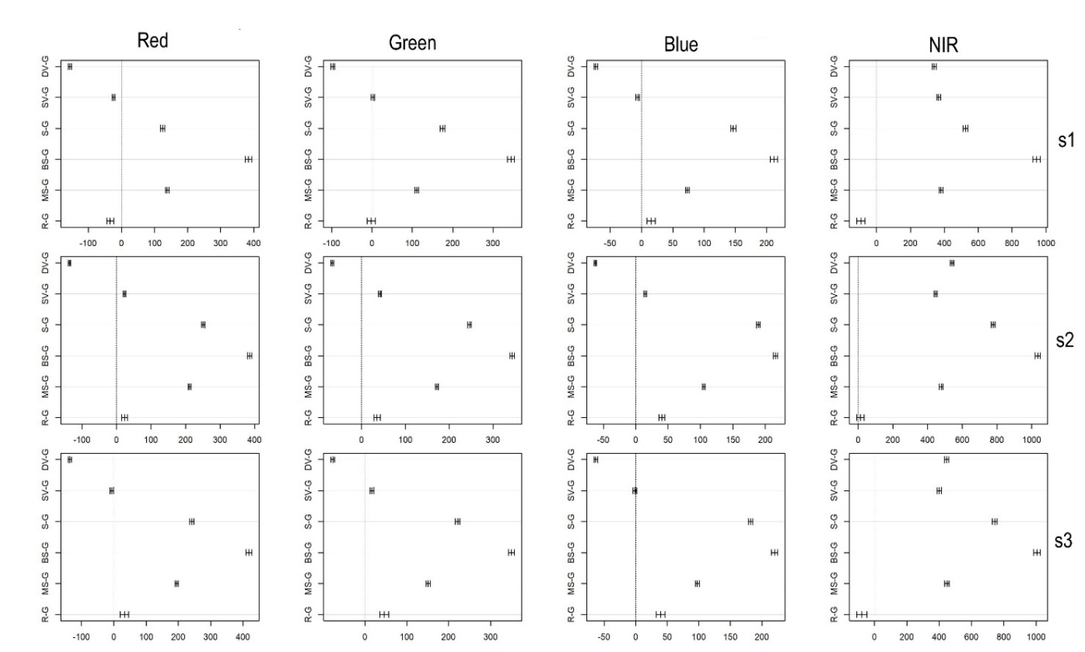
Although effect sizes were not calculated to land cover pairs of the multiclass approach, confidence intervals provided valuable information on the differences. Usually, all pairs had significant differences, and the confidence intervals were within a small range except some land cover categories: gullies and stressed vegetation and roads had non-significant differences in RGB bands (mostly in red and green bands), but the NIR band always reported significant differences. However, according to the confidence intervals, NIR band was so successful to discriminate the roads and gullies: 95% confidence ranges were close to the “zero” line, which indicated non-significance (Figure 9). This was not signed by the p-values (all of them were p < 0.001); however, if we use confidence ranges and their distance from zero as an effect size, these cases indicate low values with lower efficiency to distinguish categories. However, despite the critics of the statistical evaluation, considering the results, we can accept that reference dataset contained reliable data about land cover categories, and presumably, can be used in classification models.

As different classifiers were applied, we evaluated their overall performance. RF and SVM are robust algorithms, as data distribution does not bias the results, i.e., outliers have only slight effect on the classification accuracy, while LDA assumes multivariate normality and balanced element number in the categories [89,90]. This was also true in our study as both RFb and SVMm outperformed the LDA. But it should be noted, LDAb had better classification results in case of binary approach than RFm and SVMm. Multiclass classifications’ OA values were below the binary; thus, one can think that it is more reasonable to use only categories when possible, i.e., in our case the gully and non-gully categories. Beygelzimer et al. [91] also found that the binary approach can perform better than the multiclass. To gain this result, the authors developed a new “weighted one-against-all” method. However, in our case, the reality is that this result is only generally true, on category level, the multiclass approach was more efficient regarding the gully identification. These findings are in high agreement with those of Allwein et al. 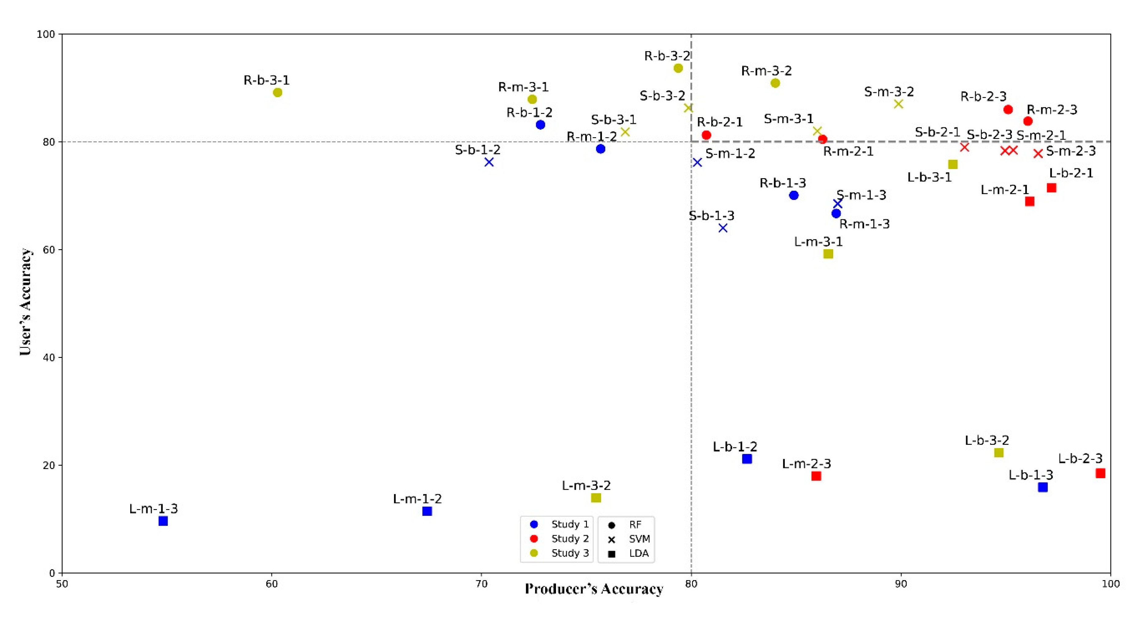[92]. Our findings revealed that multiclass solutions with the 7-class classification had better performance, only two binary approach models were in the best 80% quadrant (delineated by UA and PA) with RF and SVM classifiers. LDA’s performance varied and models provided ambiguous results: first three within the 36 models were LDA using the binary approach, and the second best was an LDA in the multiclass types based on the PA; however, the corresponding UA values were very low (e.g., the best PA, 99.51%, belonged to L-b-2-3 and the UA was only 18.5%). Thus, in these study areas with these reference datasets, we found that LDA models were severely biased by the outliers, while RF and SVM overcame this issue and provided accurate outcomes with the same input train data.

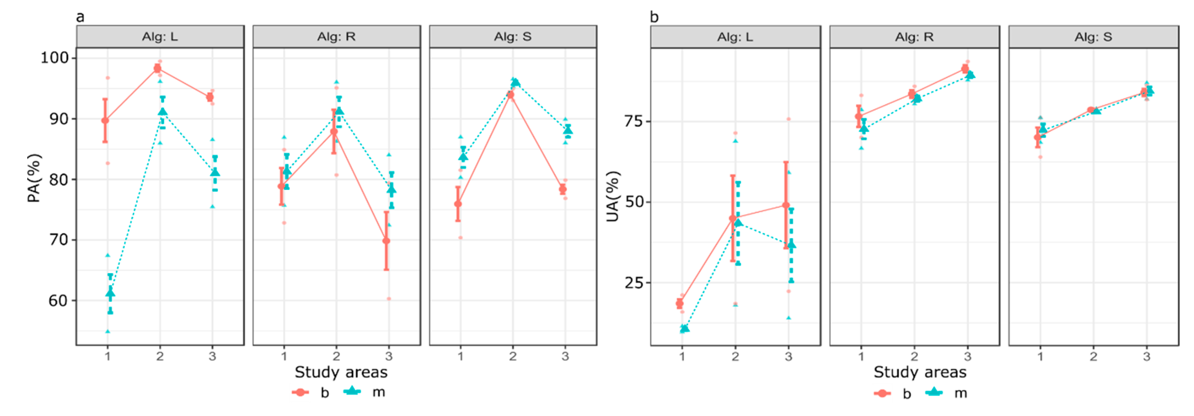
We applied GLM to investigate the reliability of the train datasets with applying the models trained with them on two other areas. All areas were similar regarding their spectral characteristics, but the six combinations revealed that in case of Study area #2, PAs were above the other two areas, but it was not true for UAs where Study area #3 had the largest values (Table 5 and Table 6; Figure 9). Although the study areas had differences regarding the reference data, both RF and SVM provided PAs and UAs above 75%, which is relatively high, considering the lack of ancillary data (e.g., a digital elevation model). LDA models had large dependency on training data quality and, therefore, the error of commissions was very large (medians indicated >50% errors).

GLM revealed the multivariate effects on PA and UA and confirmed the relevance of the classification algorithms. Number of classes (binary or multiclass) did not have significant effect; although results of 10-fold cross-validation suggested that binary classifications had better performance, class-level comparisons did not support this finding in case of gullies. Nevertheless, this study showed that space-borne images like SPOT-7 can be successfully applied to automatically detect gullies using relevant ML algorithms. Although the spectral bands of SPOT-7 played a key role in discriminating gullies among other land cover categories, pan sharpening too, to some extent, contributed to successful extraction of gullies. Automatic detection of gullies with remote sensing is a challenge, because gullies do not generally differ from the surfaces they incise [23]. As a result, visual interpretation of high-resolution images has been preferred for monitoring gullies over large areas. On a country scale, Mararakanye and Le Roux [27] performed visual interpretation of SPOT-5 image to monitor gully erosion in South Africa. Recently, Karydas and Panagos [93] performed a preliminary assessment on the presence of ephemeral gullies in Greece through visual interpretation of Google Earth images. Undoubtedly, there is a need for more reliable methods, which can help to automatically identify the areas affected by gullies [22,23]. This in turn ensures consistent monitoring of gully development over space and time. The use of appropriate ML algorithms and satellite images seems to be adequate for these surveys, but without digital elevation models (DEMs), the simple classifications can be flawed. However, in areas where gullies can be identified visually, the spectral reflectance permits the discrimination of gullies from other land cover categories, as was the case in the present study. For example, most gullies were located on bare soil surface but with the improved geometric resolution, the applied pan-sharpened product successfully discriminated gullies from bare soil although there is still a room for improvement. Where available, future research should incorporate ancillary data (i.e., DEM) to accurately discern gullies from paved/unpaved road network. A major limitation in this study was to discriminate unpaved roads from bare soil and exposed rocks. Instead, these land cover types were grouped into one class, called mixed bare soil (MS), but this did not affect gully, the target class. Although this study was conducted in small areas, the methodology applied could be adopted for application in larger areas.

5. Conclusions

Gully erosion is a crucial problem confronting sustainable agriculture today and cannot be left unabated, if sustainable agriculture is to be achieved. This study employed three commonly used ML algorithms including DA, SVM, and RF in gully feature extraction. Using these ML algorithms, we relied on two different approaches of class number: binary and multiclass. Based on the findings of this study, we drew the following conclusions:

• Despite having a small number of bands (RGB and NIR), the pan-sharpened product from SPOT-7 multispectral image successfully discriminated gullies (with OAs >95%).
• Repeated k-fold cross-validation was an efficient tool to analyze the representativeness of the reference data as reflected in different classification algorithms. It showed that the binary approach performed better (i.e., higher OAs with narrow interquartile ranges) with all classifiers than the multiclass approach.
• GLM effectively identified the biasing factors of a given class, in this case gullies, accuracy metrics (PA and UA), with the option of statistical interaction Accordingly, we revealed that algorithms performed differently with the binary or multiclass approach in case of PA, while there was no interaction in case of UA, i.e., the number of classes did not influence UAs in the function of different classifiers.
• LDA can accurately identify gullies at least from the PA’s perspective, but had usually low corresponding UA values.
• SVM and RF showed better performance compared to LDA in identifying gullies, usually with >80% of PA and UA in different areas.

Overall, we conclude that the application of different study areas for training and prediction ensures independent circumstances for models, which allow to assess the possibilities of generalization of the case studies. OAs can be misleading as the accuracy can be different at class level. In our case, the classifiers showed best performance with the binary approach, according to the OA, but the multiclass approach was more efficient in gully identification based on the PA and UA on class level. Our aim was to obtain the best representation of gullies; therefore, we suggest the use of several classes instead of only two classes (i.e., binary) for better gully feature extraction.

References

1. FAO Soil Erosion: The Gratest Challenge for Sustainable Soil Management. Available online: http://www.fao.org/3/ca4395en/ca4395en.pdf (accessed on 13 January 2020).
2. Valentin, C.; Poesen, J.; Li, Y. Gully erosion: Impacts, factors and control. Catena 2005, 63, 132–153. [Google Scholar] [CrossRef]
3. Blake, W.H.; Rabinovich, A.; Wynants, M.; Kelly, C.; Nasseri, M.; Ngondya, I.; Patrick, A.; Mtei, K.; Munishi, L.; Boeckx, P.; et al. Soil erosion in East Africa: An interdisciplinary approach to realising pastoral land management change. Environ. Res. Lett. 2018, 13, 1–12. [Google Scholar] [CrossRef] [Green Version]
4. Rodrigo-Comino, J.; Neumann, M.; Remke, A.; Ries, J.B. Assessing environmental changes in abandoned german vineyards. Understanding key issues for restoration management plans. Hung. Geogr. Bull. 2018, 67, 319–332. [Google Scholar] [CrossRef] [Green Version]
5. Kakembo, V.; Rowntree, K.M. The relationship between land use and soil erosion in the communal lands near Peddie town, Eastern Cape, South Africa. L. Degrad. Dev. 2003, 14, 39–49. [Google Scholar] [CrossRef]
6. Gholami, V. The influence of deforestation on runoff generation and soil erosion (Case study: Kasilian Watershed). J. For. Sci. 2013, 59, 272–278. [Google Scholar] [CrossRef] [Green Version]
7. Kertész, A.; Křeček, J. Landscape degradation in the world and in Hungary. Hung. Geogr. Bull. 2019, 68, 201–221. [Google Scholar] [CrossRef] [Green Version]
8. Phinzi, K.; Ngetar, N.S. Land use/land cover dynamics and soil erosion in the Umzintlava catchment (T32E), Eastern Cape, South Africa. Trans. R. Soc. S. Afr. 2019, 74, 223–237. [Google Scholar] [CrossRef]
9. Jakab, G.; Szabó, J.; Szalai, Z. A review on sheet erosion measurements in Hungary. J. Landsc. Ecol. 2015, 13, 89–103. [Google Scholar]
10. Arabameri, A.; Chen, W.; Loche, M.; Zhao, X.; Li, Y.; Lombardo, L.; Cerda, A.; Pradhan, B.; Bui, D.T. Comparison of machine learning models for gully erosion susceptibility mapping. Geosci. Front. 2019, 1–12. [Google Scholar] [CrossRef]
11. Poesen, J.; Vandekerckhove, L.; Nachtergaele, J.; Oostwoud Wijdenes, D.; Verstraeten, G.; van Wesemael, B. Gully erosion in dryland environments. In Dryland Rivers: Hydrology and Geomorphology of Semi-Arid; Bull, L.J., Kirkby, M.J., Eds.; John Wiley & Sons Ltd.: Chichester, UK, 2002; pp. 229–262. [Google Scholar]
12. Takken, I.; Croke, J.; Lane, P. Thresholds for channel initiation at road drain outlets. Catena 2008, 75, 257–267. [Google Scholar] [CrossRef]
13. Zgłobicki, W.; Baran-Zgłobicka, B.; Gawrysiak, L.; Telecka, M. The impact of permanent gullies on present-day land use and agriculture in loess areas (E. Poland). Catena 2015, 126, 28–36. [Google Scholar] [CrossRef]
14. Garland, G.G.; Hoffman, M.T.; Todd, S. Soil Degradation: A National Review of Land Degradation in South Africa; South African National Biodiversity Institute: Pretoria, South Africa, 2000; pp. 69–107. [Google Scholar]
15. Hoffman, T.; Ashwell, A. Nature Divided: Land Degradation in South Africa; University of Cape Town Press: Lansdowne, South Africa, 2001; p. 179. [Google Scholar]
16. De Villiers, M.C.; Nell, J.P.; Barnard, R.O.; Henning, A. Salt-Affected Soils: South Africa. Available online: https://www.researchgate.net/profile/Anoop_Srivastava7/post/I_am_looking_for_a_recent_soil_salinity_map_of_Africa/attachment/59d654de79197b80779ac3f2/AS:523166767423489@1501744085582/download/faosodicrza+%283%29.doc (accessed on 15 February 2020).
17. Phinzi, K.; Ngetar, N.S. Mapping soil erosion in a quaternary catchment in Eastern Cape using geographic information system and remote sensing. S. Afr. J. Geomatics 2017, 6, 11–29. [Google Scholar] [CrossRef] [Green Version]
18. Campbell, J.B.; Wynne, R.H. Introduction to Remote Sensing; Guilford Press: New York, NY, USA, 2011; p. 718. [Google Scholar]
19. Lillesand, T.; Kiefer, R.W.; Chipman, J. Remote Sensing and Image Interpretation, 7th ed.; John Wiley & Sons: New York, NY, USA, 2015; p. 768. [Google Scholar]
20. Richards, J.A.; Xiuping, J. Remote Sensing Digital Image Analysis: An Introduction, 4th ed.; Springer: Berlin, Germany, 2006; p. 494. [Google Scholar]
21. Fulajtár, E. Identification of severely eroded soils from remote sensing data tested in rišňovce, Slovakia. In Proceedings of the 10th International Soil Conservation Meeting, Indianapolis, IN, USA, 24–29 May 1999. [Google Scholar]
22. Vrieling, A.; Rodrigues, S.C.; Bartholomeus, H.; Sterk, G. Automatic identification of erosion gullies with ASTER imagery in the Brazilian Cerrados. Int. J. Remote Sens. 2007, 28, 2723–2738. [Google Scholar] [CrossRef]
23. D’Oleire-Oltmanns, S.; Marzolff, I.; Tiede, D.; Blaschke, T. Detection of gully-affected areas by applying object-based image analysis (OBIA) in the region of Taroudannt, Morocco. Remote Sens. 2014, 6, 8287–8309. [Google Scholar] [CrossRef] [Green Version]
24. Bertalan, L.; Túri, Z.; Szabó, G. UAS photogrammetry and object-based image analysis (GEOBIA): Erosion monitoring at the Kazár badland, Hungary. Landsc. Environ. 2016, 10, 169–178. [Google Scholar] [CrossRef] [Green Version]
25. Pourghasemi, H.R.; Yousefi, S.; Kornejady, A.; Cerdà, A. Performance assessment of individual and ensemble data-mining techniques for gully erosion modeling. Sci. Total Environ. 2017, 609, 764–775. [Google Scholar] [CrossRef] [Green Version]
26. Žížala, D.; Juřicová, A.; Zádorová, T.; Zelenková, K.; Minařík, R. Mapping soil degradation using remote sensing data and ancillary data: South-East Moravia, Czech Republic. Eur. J. Remote Sens. 2019, 52, 108–122. [Google Scholar] [CrossRef] [Green Version]
27. Mararakanye, N.; Le Roux, J.J. Gully location mapping at a national scale for South Africa. S. Afr. Geogr. J. 2012, 94, 208–218. [Google Scholar] [CrossRef]
28. Chen, Y.; Lin, Z.; Zhao, X.; Wang, G.; Gu, Y. Deep learning-based classification of hyperspectral data. IEEE J. Sel. Top. Appl. Earth Obs. Remote Sens. 2014, 7, 2094–2107. [Google Scholar] [CrossRef]
29. Kussul, N.; Lavreniuk, M.; Skakun, S.; Shelestov, A. Deep learning classification of land cover and crop types using remote sensing data. IEEE Geosci. Remote Sens. Lett. 2017, 14, 778–782. [Google Scholar] [CrossRef]
30. Vetrivel, A.; Gerke, M.; Kerle, N.; Nex, F.; Vosselman, G. Disaster damage detection through synergistic use of deep learning and 3D point cloud features derived from very high resolution oblique aerial images, and multiple-kernel-learning. ISPRS J. Photogramm. Remote Sens. 2018, 140, 45–59. [Google Scholar] [CrossRef]
31. Ball, J.E.; Anderson, D.T.; Chan, C.S. Comprehensive survey of deep learning in remote sensing: Theories, tools, and challenges for the community. J. Appl. Remote Sens. 2017, 11, 1–54. [Google Scholar] [CrossRef] [Green Version]
32. Zhang, L.; Xia, G.S.; Wu, T.; Lin, L.; Tai, X.C. Deep Learning for Remote Sensing Image Understanding. J. Sensors 2016, 4, 22–40. [Google Scholar] [CrossRef]
33. Chen, G.; Zhang, X.; Wang, Q.; Dai, F.; Gong, Y.; Zhu, K. Symmetrical dense-shortcut deep fully convolutional networks for semantic segmentation of very-high-resolution remote sensing images. IEEE J. Sel. Top. Appl. Earth Obs. Remote Sens. 2018, 11, 1633–1644. [Google Scholar] [CrossRef]
34. Ma, L.; Liu, Y.; Zhang, X.; Ye, Y.; Yin, G.; Johnson, B.A. Deep learning in remote sensing applications: A meta-analysis and review. ISPRS J. Photogramm. Remote Sens. 2019, 152, 166–177. [Google Scholar] [CrossRef]
35. Szabó, L.; Burai, P.; Deák, B.; Dyke, G.J.; Szabó, S. Assessing the efficiency of multispectral satellite and airborne hyperspectral images for land cover mapping in an aquatic environment with emphasis on the water caltrop (Trapa natans). Int. J. Remote Sens. 2019, 40, 5192–5215. [Google Scholar] [CrossRef]
36. Manandhar, S.; Dev, S.; Lee, Y.H.; Meng, Y.S.; Winkler, S. A Data-Driven Approach for Accurate Rainfall Prediction. IEEE Trans. Geosci. Remote Sens. 2019, 57, 9323–9331. [Google Scholar] [CrossRef] [Green Version]
37. Kai, W.; Jinyi, G.; Nan, Z. Evaluation on Water Source Conservation Capacity of West Liaohe River Basin Based on Invest Model. In Proceedings of the 2019 International Conference on Smart Grid and Electrical Automation (ICSGEA), IEEE, Xiangtan, China, 10–11 August 2019; pp. 443–447. [Google Scholar]
38. Drake, J.M.; Randin, C.; Guisan, A. Modelling ecological niches with support vector machines. J. Appl. Ecol. 2006, 43, 424–432. [Google Scholar] [CrossRef]
39. Goldblatt, R.; You, W.; Hanson, G.; Khandelwal, A.K. Detecting the boundaries of urban areas in India: A dataset for pixel-based image classification in google earth engine. Remote Sens. 2016, 8, 634. [Google Scholar] [CrossRef] [Green Version]
40. Gautam, R.; Panigrahi, S.; Franzen, D.; Sims, A. Residual soil nitrate prediction from imagery and non-imagery information using neural network technique. Biosyst. Eng. 2011, 110, 20–28. [Google Scholar] [CrossRef]
41. Bui, D.T.; Shirzadi, A.; Shahabi, H.; Chapi, K.; Omidavr, E.; Pham, B.T.; Asl, D.T.; Khaledian, H.; Pradhan, B.; Panahi, M.; et al. A novel ensemble artificial intelligence approach for gully erosion mapping in a semi-arid watershed (Iran). Sensors 2019, 19, 2444. [Google Scholar]
42. Chen, L.; Ren, C.; Li, L.; Wang, Y.; Zhang, B.; Wang, Z.; Li, L. A comparative assessment of geostatistical, machine learning, and hybrid approaches for mapping topsoil organic carbon content. ISPRS Int. J. Geo-Inf. 2019, 8, 174. [Google Scholar] [CrossRef] [Green Version]
43. Hateffard, F.; Dolati, P.; Heidari, A.; Zolfaghari, A.A. Assessing the performance of decision tree and neural network models in mapping soil properties. J. Mt. Sci. 2019, 16, 1833–1847. [Google Scholar] [CrossRef]
44. Adam, E.; Mutanga, O.; Odindi, J.; Abdel-Rahman, E.M. Land-use/cover classification in a heterogeneous coastal landscape using RapidEye imagery: Evaluating the performance of random forest and support vector machines classifiers. Int. J. Remote Sens. 2014, 35, 3440–3458. [Google Scholar] [CrossRef]
45. Phinzi, K.; Ngetar, N.S. The assessment of water-borne erosion at catchment level using GIS-based RUSLE and remote sensing: A review. Int. Soil Water Conserv. Res. 2019, 7, 27–46. [Google Scholar] [CrossRef]
46. Maxwell, A.E.; Warner, T.A.; Fang, F. Implementation of machine-learning classification in remote sensing: An applied review. Int. J. Remote Sens. 2018, 39, 2784–2817. [Google Scholar] [CrossRef] [Green Version]
47. Enyedi, P.; Pap, M.; Kovács, Z.; Takács-Szilágyi, L.; Szabó, S. Efficiency of local minima and GLM techniques in sinkhole extraction from a LiDAR-based terrain model. Int. J. Digit. Earth 2019, 12, 1067–1082. [Google Scholar] [CrossRef]
48. Shruthi, R.B.V.; Kerle, N.; Jetten, V. Object-based gully feature extraction using high spatial resolution imagery. Geomorphology 2011, 134, 260–268. [Google Scholar] [CrossRef]
49. Wang, F.; Zhen, Z.; Wang, B.; Mi, Z. Comparative study on KNN and SVM based weather classification models for day ahead short term solar PV power forecasting. Appl. Sci. 2018, 8, 28. [Google Scholar] [CrossRef] [Green Version]
50. Maurer, T. How to pan-sharpen images using the gram-schmidt pan-sharpen method—A recipe. In Proceedings of the ISPRS Hannover Workshop, Hannover, Germany, 21–24 May 2013. [Google Scholar]
51. Abriha, D.; Kovács, Z.; Ninsawat, S.; Bertalan, L.; Balázs, B.; Szabó, S. Identification of roofing materials with discriminant function analyand random forest classifiers on pan-sharpened worldview-2 imagery—A comparison. Hung. Geogr. Bull. 2018, 67, 375–392. [Google Scholar] [CrossRef] [Green Version]
52. Grochala, A.; Kedzierski, M. A method of panchromatic image modification for satellite imagery data fusion. Remote Sens. 2017, 9, 639. [Google Scholar] [CrossRef] [Green Version]
53. Ge, W.; Cheng, Q.; Tang, Y.; Jing, L.; Gao, C. Lithological classification using Sentinel-2A data in the Shibanjing ophiolite complex in Inner Mongolia, China. Remote Sens. 2018, 10, 638. [Google Scholar] [CrossRef] [Green Version]
54. Breiman, L. Random forests. Mach. Learn. 2001, 45, 5–32. [Google Scholar] [CrossRef] [Green Version]
55. Rodriguez-Galiano, V.F.; Ghimire, B.; Rogan, J.; Chica-Olmo, M.; Rigol-Sanchez, J.P. An assessment of the effectiveness of a random forest classifier for land-cover classification. ISPRS J. Photogramm. Remote Sens. 2012, 67, 93–104. [Google Scholar] [CrossRef]
56. Shahabi, H.; Jarihani, B.; Tavakkoli Piralilou, S.; Chittleborough, D.; Avand, M.; Ghorbanzadeh, O. A Semi-Automated Object-Based Gully Networks Detection Using Different Machine Learning Models: A Case Study of Bowen Catchment, Queensland, Australia. Sensors 2019, 19, 4893. [Google Scholar] [CrossRef] [Green Version]
57. Burai, P.; Deák, B.; Valkó, O.; Tomor, T. Classification of herbaceous vegetation using airborne hyperspectral imagery. Remote Sens. 2015, 7, 2046–2066. [Google Scholar] [CrossRef] [Green Version]
58. Sabat-tomala, A.; Raczko, E. Comparison of Support Vector Machine and Random Forest Algorithms for Invasive and Expansive Species Classification Using Airborne Hyperspectral Data. Remote Sens. 2020, 12, 516. [Google Scholar] [CrossRef] [Green Version]
59. Shruthi, R.B.V.; Kerle, N.; Jetten, V.; Stein, A. Object-based gully system prediction from medium resolution imagery using Random Forests. Geomorphology 2014, 216, 283–294. [Google Scholar] [CrossRef]
60. Phinzi, K.; Ngetar, N.S.; Ebhuoma, O. Soil erosion risk assessment in the Umzintlava catchment (T32E), Eastern Cape, South Africa, using RUSLE and random forest algorithm. S. Afr. Geogr. J. 2020, 1–24. [Google Scholar] [CrossRef]
61. Szatmári, G.; Pásztor, L. Comparison of various uncertainty modelling approaches based on geostatistics and machine learning algorithms. Geoderma 2019, 337, 1329–1340. [Google Scholar] [CrossRef]
62. Deng, S.; Katoh, M.; Yu, X.; Hyyppä, J.; Gao, T. Comparison of tree species classifications at the individual tree level by combining ALS data and RGB images using different algorithms. Remote Sens. 2016, 8, 1034. [Google Scholar] [CrossRef] [Green Version]
63. Balázs, B.; Bíró, T.; Dyke, G.; Singh, S.K.; Szabó, S. Extracting water-related features using reflectance data and principal component analysis of Landsat images. Hydrol. Sci. J. 2018, 63, 269–284. [Google Scholar] [CrossRef]
64. Vapnik, V. The Nature of Statistical Learning Theory, 2nd ed.; Springer: New York, NY, USA, 2013; p. 311. [Google Scholar]
65. Brenning, A. Spatial prediction models for landslide hazards: Review, comparison and evaluation. Nat. Hazards Earth Syst. Sci. 2005, 5, 853–862. [Google Scholar] [CrossRef]
66. Otukei, J.R.; Blaschke, T. Land cover change assessment using decision trees, support vector machines and maximum likelihood classification algorithms. Int. J. Appl. Earth Obs. Geoinf. 2010, 12, 27–31. [Google Scholar] [CrossRef]
67. De Boissieu, F.; Sevin, B.; Cudahy, T.; Mangeas, M.; Chevrel, S.; Ong, C.; Rodger, A.; Maurizot, P.; Laukamp, C.; Lau, I.; et al. Regolith-geology mapping with support vector machine: A case study over weathered Ni-bearing peridotites, New Caledonia. Int. J. Appl. Earth Obs. Geoinf. 2018, 64, 377–385. [Google Scholar] [CrossRef]
68. Wu, Y.; Zhang, X. Object-Based tree species classification using airborne hyperspectral images and LiDAR data. Forests 2020, 11, 32. [Google Scholar] [CrossRef] [Green Version]
69. Gholizadeh, A.; Borůvka, L.; Saberioon, M.; Vašát, R. A memory-based learning approach as compared to other data mining algorithms for the prediction of soil texture using diffuse reflectance spectra. Remote Sens. 2016, 8, 341. [Google Scholar] [CrossRef] [Green Version]
70. Lantz, B. Machine Learning with R: Expert Techniques for Predictive Modeling to Solve All your Data Analysis Problems, 3rd ed.; Packt Publishing Ltd: Birmingham, UK, 2015; p. 427. [Google Scholar]
71. Harrell, F.E.; Lee, K.L. A comparison of the discrimination of discriminant analysis and logistic regression under multivariate normality. Biostat. Stat. Biomed. Public Heal. Environ. Sci. 1985, 1985, 333–343. [Google Scholar]
72. Tharwat, A. Linear vs. quadratic discriminant analysis classifier: A tutorial. Int. J. Appl. Pattern Recognit. 2016, 3, 145–180. [Google Scholar] [CrossRef]
73. Dube, T.; Mutanga, O.; Sibanda, M.; Seutloali, K.; Shoko, C. Use of Landsat series data to analyse the spatial and temporal variations of land degradation in a dispersive soil environment: A case of King Sabata Dalindyebo local municipality in the Eastern Cape Province, South Africa. Phys. Chem. Earth 2017, 100, 112–120. [Google Scholar] [CrossRef]
74. Machine Learning Mastery. Available online: https://machinelearningmastery.com/ (accessed on 21 February 2020).
75. Heckel, K.; Urban, M.; Schratz, P.; Mahecha, M.D.; Schmullius, C. Predicting Forest Cover in Distinct Ecosystems: The Potential of Multi-Source Sentinel-1 and -2 Data Fusion. Remote Sens. 2020, 12, 302. [Google Scholar] [CrossRef] [Green Version]
76. Congalton, R.G. A review of assessing the accuracy of classifications of remotely sensed data. Remote Sens. Environ. 1991, 37, 35–46. [Google Scholar] [CrossRef]
77. Singh, S.K.; Srivastava, P.K.; Szabó, S.; Petropoulos, G.P.; Gupta, M.; Islam, T. Landscape transform and spatial metrics for mapping spatiotemporal land cover dynamics using Earth Observation data-sets. Geocarto Int. 2017, 32, 113–127. [Google Scholar] [CrossRef] [Green Version]
78. Lamine, S.; Petropoulos, G.P.; Singh, S.K.; Szabó, S.; Bachari, N.E.I.; Srivastava, P.K.; Suman, S. Quantifying land use/land cover spatio-temporal landscape pattern dynamics from Hyperion using SVMs classifier and FRAGSTATS®. Geocarto Int. 2018, 33, 862–878. [Google Scholar] [CrossRef]
79. Congalton, R.G.; Green, K. Assessing the Accuracy of Remotely Sensed Data: Principles and Practices, 3rd ed.; CRC Press: Boca Raton, FL, USA, 2019; p. 319. [Google Scholar]
80. Mohd Razali, N.; Bee Wah, Y. Power comparisons of Shapiro-Wilk, Kolmogorov-Smirnov, Lilliefors and Anderson-Darling tests. J. Stat. Model. Anal. 2011, 2, 21–33. [Google Scholar]
81. Field, A.; Miles, J.; Field, Z. Discovering Statistics Using R; SAGE Publications: London, UK, 2012; p. 957. [Google Scholar]
82. Tallarida, R.J.; Murray, R.B. Dunnett’s Test (Comparison with a Control). In Manual of Pharmacologic Calculations, 2nd ed.; Springer: New York, NY, USA, 1987; pp. 145–148. [Google Scholar]
83. Levine, T.R.; Hullett, C.R. Eta Squared, Partial Eta Squared, and Misreporting of Effect Size in Communication Research. Hum. Commun. Res. 2002, 28, 612–625. [Google Scholar] [CrossRef]
84. The R Project for Statistical Computing. Available online: https://www.r-project.org (accessed on 21 February 2020).
85. Mair, P.; Wilcox, R. Robust statistical methods in R using the WRS2 package. Behav. Res. Methods 2019, 52, 1–25. [Google Scholar] [CrossRef]
86. Jamovi. Available online: https://www.jamovi.org/about.html (accessed on 21 February 2020).
87. Gallucci, M. GMLj: General Analysis for Linear Models. Available online: https://gamlj.github.io (accessed on 21 February 2020).
88. Szabó, S.; Bertalan, L.; Kerekes, Á.; Novák, T.J. Possibilities of land use change analysis in a mountainous rural area: A methodological approach. Int. J. Geogr. Inf. Sci. 2016, 30, 708–726. [Google Scholar] [CrossRef] [Green Version]
89. Belgiu, M.; Drăgu, L. Random forest in remote sensing: A review of applications and future directions. ISPRS J. Photogramm. Remote Sens. 2016, 114, 24–31. [Google Scholar] [CrossRef]
90. Xiong, K.; Adhikari, B.R.; Stamatopoulos, C.A.; Zhan, Y.; Wu, S.; Dong, Z.; Di, B. Comparison of Different Machine Learning Methods for Debris Flow Susceptibility Mapping: A Case Study in the Sichuan Province, China. Remote Sens. 2020, 12, 1–20. [Google Scholar] [CrossRef]
91. Beygelzimer, A.; Langford, J.; Zadrozny, B. Weighted One-Against-All. Am. Assoc. Artif. Intell. 2004, 2, 720–725. [Google Scholar]
92. Allwein, E.L.; Schapire, R.E.; Singer, Y. Reducing multiclass to binary: A unifying approach for margin classifiers. J. Mach. Learn. Res. 2000, 1, 113–141. [Google Scholar]
93. Karydas, C.; Panagos, P. Towards an Assessment of the Ephemeral Gully Erosion Potential in Greece Using Google Earth. Water 2020, 12, 603. [Google Scholar] [CrossRef] [Green Version]
Figure 1. Geographical location of the study area.
Ijgi 09 00252 g001
Figure 2. Distribution of reflectance values of Systeme Pour l’Observation de la Terre (SPOT-7) image by bands (red, green, blue (RGB) and near infrared (NIR)), study areas (s1–s3) and classification categories (NG: non-gully, G: gully).
Ijgi 09 00252 g002
Figure 3. Distribution of reflectance values of SPOT-7 image by bands (RGV+NIR), study areas (s1–s3), and classification categories (DV: dense vegetation, SV: stressed vegetation, S: settlement, G: gully, BS: bare soil, MS: mixed bare soil, R: road).
Ijgi 09 00252 g003
Figure 4. Mean differences between gullies (G) and other land cover categories (mean ± 95% confidence intervals; 95% confidence intervals coinciding with 0 are not significant differences, p > 0.05; DV: dense vegetation, SV: stressed vegetation, S: settlement, BS: bare soil, MS: mixed bare soil, R: roads) by SPOT 7 bands (columns) and study areas (rows).
Ijgi 09 00252 g004
Figure 5. Classification results of the multiclass approach (DV: dense vegetation, SV: stressed vegetation, S: settlement, G: gully, BS: bare soil, MS: mixed bare soil, R: road).
Ijgi 09 00252 g005
Figure 6. Classification results of the binary approach (G: gully, NG: non-gully).
Ijgi 09 00252 g006
Figure 7. Classification results of the applied algorithms ranked by overall accuracies of 30 models (10-fold cross-validation with three repetitions) by study areas (LDA: Linear Discriminant Analysis, RF: Random Forest, SVM: Support Vector Machine; b: binary, m: multiclass).
Ijgi 09 00252 g007
Figure 8. Class level accuracy metrics of different classifications of gullies by algorithms, number of categories and study areas (S: SVM, R: RF, L: LDA; b: binary, m: multiclass; first number: number of area where the models was applied, second number: number of area where the model was trained; dashes line sections (upper right) indicate >80% accuracy quarter).
Ijgi 09 00252 g008
Figure 9. PA (a) and UA (b) values (median ± quartiles) of gullies by classification algorithms (Alg: algorithm; L: LDA, R: RF, S: SVM), number of classes (b: binary; m: multiclass) and study areas (1-3).
Ijgi 09 00252 g009