Article

Landslide Susceptibility Prediction Considering Regional Soil Erosion Based on Machine-Learning Models

1
School of Civil Engineering and Architecture, Nanchang University, Nanchang 330031, China
2
ARC Centre of Excellence for Geotechnical Science and Engineering, University of Newcastle, Newcastle, NSW 2308, Australia
3
Changjiang Institute of Survey, Planning, Design and Research Co., Ltd., Wuhan 430010, China
*
Author to whom correspondence should be addressed.
ISPRS Int. J. Geo-Inf. 2020, 9(6), 377; https://0-doi-org.brum.beds.ac.uk/10.3390/ijgi9060377
Submission received: 20 March 2020 / Revised: 26 May 2020 / Accepted: 2 June 2020 / Published: 8 June 2020
(This article belongs to the Special Issue Geospatial Approaches to Landslide Mapping and Monitoring)

Abstract

:
Soil erosion (SE) provides slide mass sources for landslide formation, and reflects long-term rainfall erosion destruction of landslides. Therefore, it is possible to obtain more reliable landslide susceptibility prediction results by introducing SE as a geology and hydrology-related predisposing factor. The Ningdu County of China is taken as a research area. Firstly, 446 landslides are obtained through government disaster survey reports. Secondly, the SE amount in Ningdu County is calculated and nine other conventional predisposing factors are obtained under both 30 m and 60 m grid resolutions to determine the effects of SE on landslide susceptibility prediction. Thirdly, four types of machine-learning predictors with 30 m and 60 m grid resolutions—C5.0 decision tree (C5.0 DT), logistic regression (LR), multilayer perceptron (MLP) and support vector machine (SVM)—are applied to construct the landslide susceptibility prediction models considering the SE factor as SE-C5.0 DT, SE-LR, SE-MLP and SE-SVM models; C5.0 DT, LR, MLP and SVM models with no SE are also used for comparisons. Finally, the area under receiver operating feature curve is used to verify the prediction accuracy of these models, and the relative importance of all the 10 predisposing factors is ranked. The results indicate that: (1) SE factor plays the most important role in landslide susceptibility prediction among all 10 predisposing factors under both 30 m and 60 m resolutions; (2) the SE-based models have more accurate landslide susceptibility prediction than the single models with no SE factor; (3) all the models with 30 m resolutions have higher landslide susceptibility prediction accuracy than those with 60 m resolutions; and (4) the C5.0 DT and SVM models show higher landslide susceptibility prediction performance than the MLP and LR models.

1. Introduction

Landslides are one of the most common geological disasters worldwide, costing many human lives and incurring economic losses every year [1,2,3,4,5]. For example, millions of people and related property are seriously menaced by the widely distributed landslides in China [6]. Determining how to predict the spatial distribution of landslides has become a major concern of engineers all over the world. Landslide susceptibility prediction (LSP) can be defined as the spatial probability of landslide occurrence in a certain prediction unit of the study area, under the non-linear coupling effects of landslide-related basic predisposing factors with no consideration of external inducing factors [7]. Landslide susceptibility maps (LSMs) produced from LSP, one of the main visualization tools of the landslide spatial distribution, are beneficial to local engineering geological surveys and the management of landslide-prone areas [8,9,10,11].
The LSP utilizes the similar geological, terrain and other related conditions of previously occurring landslides to predict the possible location of landslide occurrence in the future [12,13]. Therefore, it is very important to select the appropriate predisposing factors that affect the evaluation of landslides for accurate and reliable LSP [14,15]. The existing literature has shown that the predisposing factors commonly used in LSP can be divided into four categories: topography factors (elevation, curvature, slope, topographic relief, etc.) [16]; basic geology factors (rock categories, geological fault, etc. ) [17]; hydrological factors (surface humidity index, distance from river network, annual rainfall, etc.) [18,19]; and surface cover factors (normalized difference vegetation index (NDVI), normalized difference built-up index (NDBI), etc.) [20,21]. The four types of predisposing factors mentioned above are mainly based on the slope structure, surface morphology, hydrological environmental and geological features of the slope. However, the influences of the soil material source on landslide evolution and the long-term process of rainfall erosion on landslide susceptibility have not been considered. In fact, slide mass sources and long-term rainfall erosion destruction are very important geology- and hydrology-related factors in landslide disasters. Hence, to better determine and explore the landslide susceptibility distribution, this study explores the effects of anew predisposing factor related to the slide mass sources and rainfall erosion on landslide occurrence based on the four types of conventional predisposing factors.
The slide mass sources of the soil landslide mainly include quaternary accumulation, such as alluvial deposits, residual and slope deposits, which are the products of regional soil erosion (SE) processes [22,23]. Generally, the SE can be used to quantitatively analyse the processes of slope erosion and destruction by long-term rainfall. This is because SE reflects the processes of erosion, destruction, separation, transportation and deposition of soil and/or other ground materials under the actions of natural forces (mainly rainfall forces) and/or the combined actions of natural forces and human activities [21]. In addition, related studies show that there is a certain correlation between SE intensity and the landslide occurrence [24], meanwhile, the SE has been used for landslide prevention [25]. Therefore, the SE can be introduced as a new predisposing factor and taken as the input variable of an LSP model.
On the basis of determining the input variables, researchers have developed many models for LSP. These models include heuristic and mathematical statistics models such as the weights of evidence model [9], certainty-based factor model [26], logistic regression (LR) [18,27], linear discriminant model [28], analytic hierarchy process method [27], etc. Recently, various machine-learning models have also been commonly introduced to implement LSP, such as decision tree (DT) [29,30,31], fuzzy logic [32], artificial neural network [28,33,34], random forest [35], support vector machine (SVM) [36,37,38], least-square support vector machine [39] and some ensemble methods [6], etc. These models connect the input variables with the landslide susceptibility index (LSI) which is regarded as the model output, through various training and testing algorithms. However, the landslide susceptibility prediction results of these types of models are significantly different, and there is no consensus on which model is the most suitable for LSP [40]. Hence, through considering the SE factor, this paper builds SE-based multilayer perceptron (MLP), LR, SVM and C5.0 DT models to address LSP. In addition, to explore and compare the influence of the SE factor on the LSP modelling, single MLP, LR, SVM and C5.0 DT models without considering the SE factor are also used to address LSP. Furthermore, SE intensity and LSP model building under different grid resolutions (30 m and 60 m) are also carried out, to discuss the effects of different prediction units associated with these input variables on the conclusions of this study. Finally, the area under the receiver operating curve (AUC) is used to evaluate the performance of SE-based and single models to obtain the optimal LSP modelling processes.

2. Materials

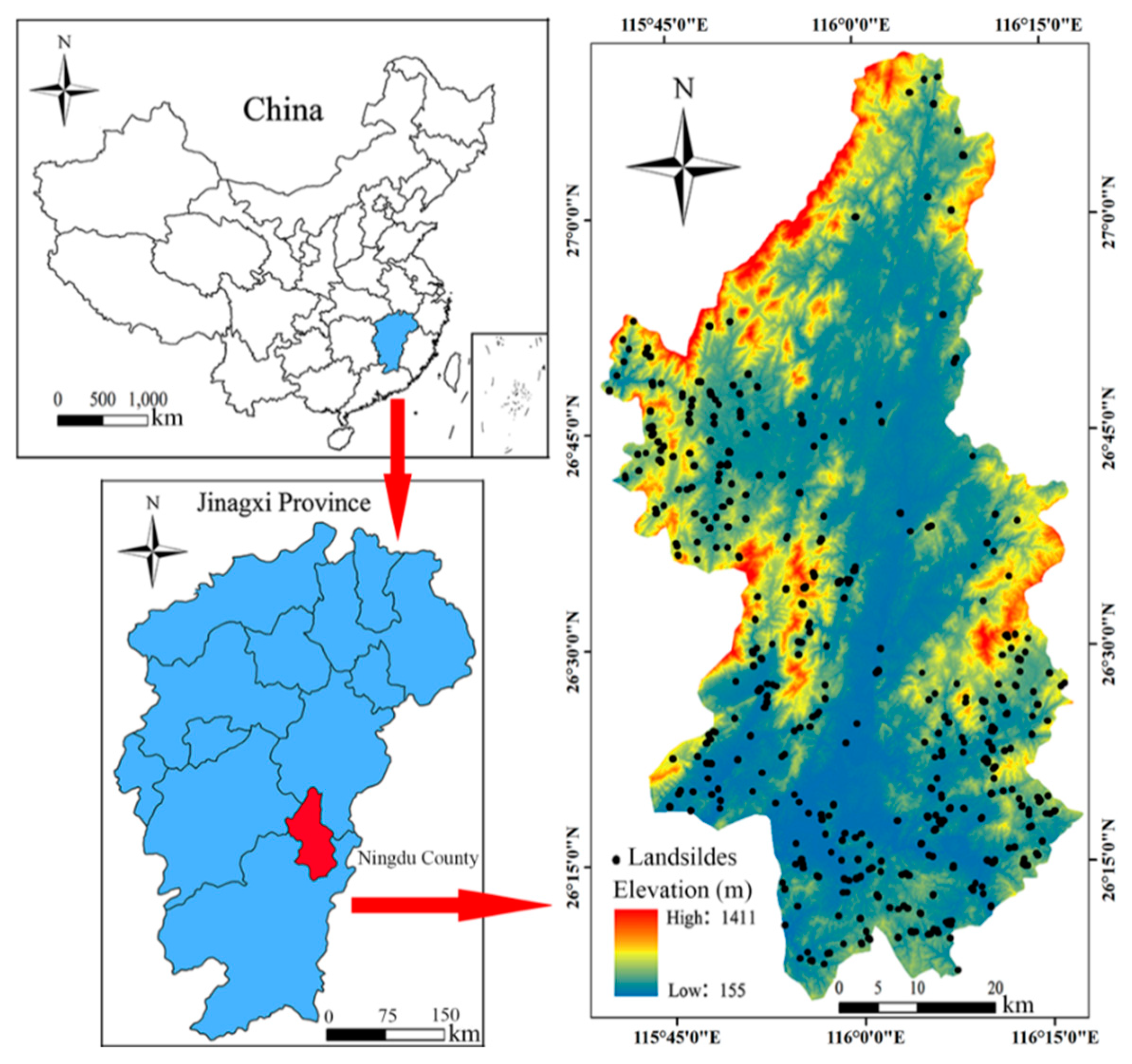
2.1. Introduction to Ningdu County and Landslide Inventory

Ningdu County (26°05′~27°08′ N, 115°40′~116°17′ E) is located in the north of Ganzhou City, Jiangxi Province of China, with a total area of 4075.5 km2, as shown in Figure 1. Ningdu County is an area with hilly and mountainous terrain. The topography of Ningdu County is high in the north and low in the south, with an altitude ranging from 155~1411 m. Ningdu County is located in zone of warm temperate climate with fully humid according to Koppen’s climate classification [41], with an average rainfall of 1500~1900 mm per year from the 1970s to 2015, where there is maximum rainfall in 2002 year with annual rainfall of 2380 mm. Rainfall processes usually occur from April to July in each year. The exposed strata in the study area include Presinian, Sinian, Cambrian, Carboniferous, Jurassic, Cretaceous and Quaternary systems. The land use types are mainly forest and bare grassland. The forest coverage rate of Ningdu County is approximately 71.8%, and the natural forest area accounts for approximately 87% of the forest area. The zonal vegetation is the central Asian zone of evergreen broad-leaved forest.
In this study, a landslide inventory map with a total of 446 landslides is produced based on the field investigation and high-resolution image interpretation from 1970 to 2003, implemented by the Ningdu Land Resources Bureau, Jiangxi Province of China. In general, these landslides are composed of the quaternary silty clay intercalated with crushed stones, the thickness of slide masses varies between 2 m and 8 m. According to the landslides classification rules presented by Hungr et al. [42], these landslides can be classified as shallow soil landslides with a movement type of clay/silt slide with main characteristics of small scale, high frequency and wide distribution. Generally speaking, these landslides are mainly distributed in the surrounding mountainous areas of Ningdu County, while less in the northern and central areas. Among these landslides, the minimum, maximum and average landslide areas are about 616 m2, 44,123 m2, and 6519 m2, respectively. The development process of these landslides is controlled by basic predisposing factors, and is induced by the heavy rainfall and unreasonable human engineering activities (such as mining of ore resources, land-use change, etc.) [43].

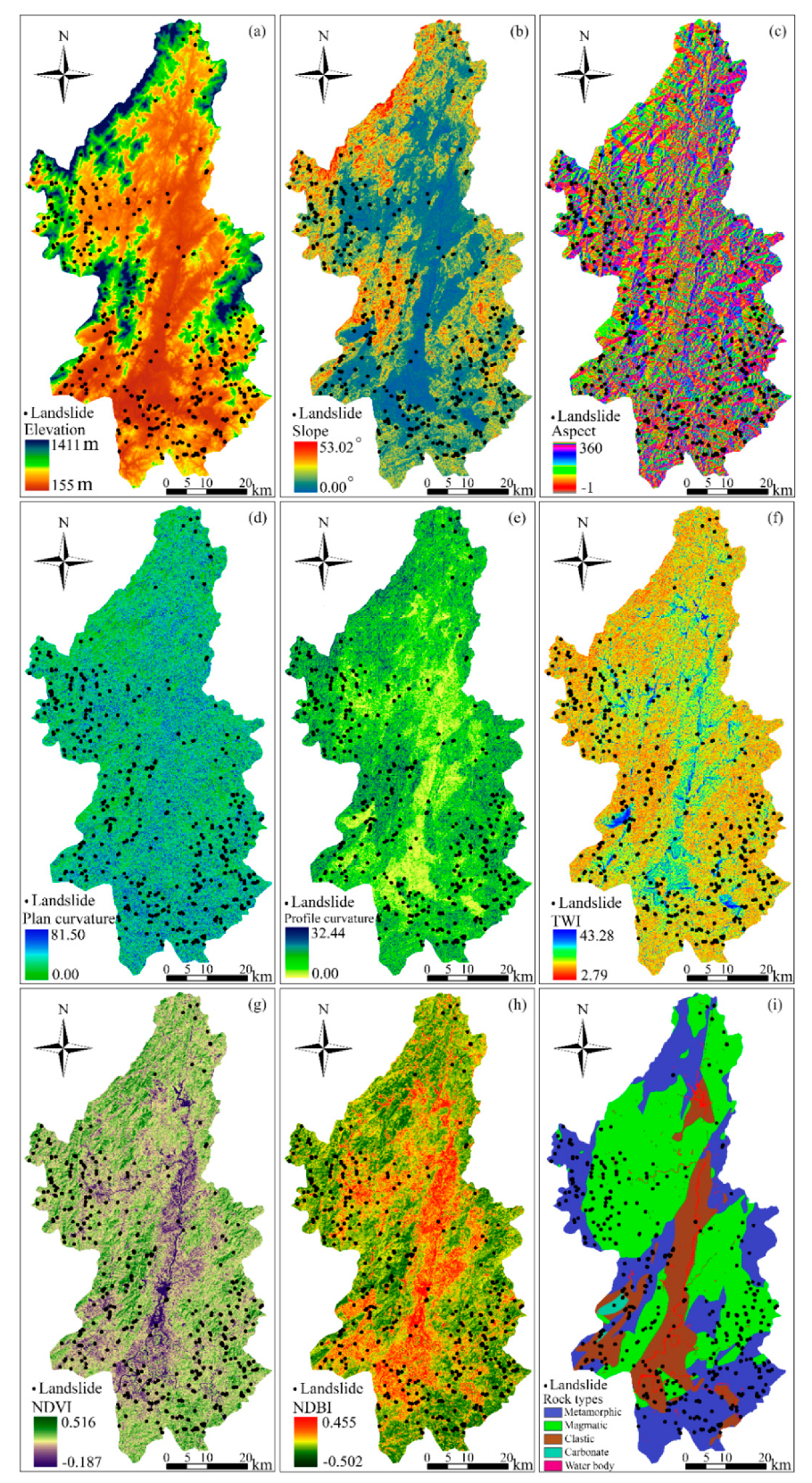
2.2. Conventional Landslide Predisposing Factors

The selection of landslide predisposing factors is uncertain due to the complexities of the landslide occurrence mechanism and the surrounding geological environments [6]. Most researchers select predisposing factors taking into account natural factors that affect landslide development (including topography and geomorphology, land cover, climate, etc.) and human engineering construction. However, the SE factor providing the material basis for landslide occurrence and reflecting long-term rainfall erosion is not considered. In fact, landslides are likely to occur in areas with serious SE phenomena. Hence, this study considers the SE factor and 9 other conventional predisposing factors for LSP (Table 1).
In this study, topography factors of elevation, slope, plan curvature, aspect, topographic wetness index (TWI) and profile curvature are calculated based on a digital elevation model (DEM) with 30 m resolution. The LSP modelling process will be complicated under grid resolution that is too high [44], while the landslide inventory and predisposing factors cannot be accurately reflected under grid resolution that is too low [45]. Hence, a grid resolution of 30 m, widely used in other studies [15,30,33,46], is selected to deal with the landslide inventory and predisposing factors considering the large area of Ningdu County. The elevation is often considered as a predisposing factor for landslides [47]. Soil and vegetation in the study area are affected by climate and temperature with increasing altitude, and the weathering effect of rocks also gradually decreases with increasing altitude. As a result, there are fewer landslide events in areas with high elevation values [48]. The slope and aspect reflect the landslide scale through the effects of external factors such as rainfall, solar radiation and land vegetation [20,49,50,51]. The plan curvature reflects the influence of topography on the convergence and divergence of water flow during the downslope flow [35]. The profile curvature is defined as a vertical plane curvature paralleling the sloping direction [52]. The TWI describes the distribution of soil moisture on the surface [53,54]. In addition, lithology is an expression of the inherent physical properties of landslide occurrence. This study generates a lithology map using a geological map with scale of 1:100,000 provided by the Land Resources Bureau of Ningdu County. The NDVI and NDBI factors are acquired from Landsat-8 Thematic Mapper (TM) images (taken on 15 October 2013, path/row 121/41 and path/row 121/42). The NDVI reflects the density of vegetation on the ground, which has an inhibitory effect on the landslides occurrence, and the NDBI represents the density of build-up area and reflects the concentration degree of human activities to some extent in Ningdu County [16].
All predisposing factors are converted into grid units with 30 m resolution in ArcGIS 10.2 software (Figure 2). The influence degrees of different subclasses of each predisposing factor on landslide occurrence can be calculated through the frequency ratio (FR) analysis, and the continuous predisposing factors are generally classified into eight subclasses for building the relationships between predisposing factors and landslides. Meanwhile, each continuous predisposing factor is classified by the Jenks natural break method, which can minimize differences within the subclass and maximize the differences between the subclasses (Table 1). Most of these landslides mainly occur in areas of elevations less than 618 m and slopes above 19.33°. The FR values of profile curvature is greater than 1 in areas above 4.71. Meanwhile, the probability of landslide occurrence is greater with NDVI values higher than 0.243 and/or with NDBI values higher than 0.292. Landslides are mainly distributed in metamorphic and carbonate rocks. In addition, a study area with SE amounts higher than 5 t/ha provides a constructive environment for landslide occurrence. In this study, the independence and collinearity test of predisposing factors are carried out, the results indicate that there are weak correlations and no multi-collinearity between factors. Hence, the FR values of all these factors can be used as input variables of LSP models.

2.3. Spatial Database Analysis

The LSP can be regarded as a binary classification problem. In this study, the 446 landslide locations are respectively converted into 3711 and 1748 landslide grid units under 30 m and 60 m grid resolutions in a raster format in ARCGIS 10.2. The landslide and non-landslide grid units are respectively set to be 1 and 0, which are taken as the output variables of the LSP models [55,56]. In the LSP processes, the landslide grid units and a same number of randomly selected non-landslide grid units are randomly divided into a training dataset and testing dataset with a ratio of 70% and 30%. In this study, the FR values of the predisposing factors are considered as the attribute features of landslide and non-landslide grid units. Hence, FR values are taken as the input dataset for LSP modelling. The 9 traditional predisposing factors are used for single models with no SE factor, while all the 10 predisposing factors are used for the SE-based models.

3. Methods

3.1. Modelling Processes Analysis

The main purpose of this study is to explore the effects of the SE factor on landslide occurrence and evaluate the importance of the SE factor in LSP modelling through comparisons of SE-based models and single models. This study has four main steps (Figure 3): (1) preparation of the model dataset, including the landslide inventory map, the 10 predisposing factors (such as SE, topography wetness index (TWI), …etc.) for SE-based models, and 9 predisposing factors for single models (such as NDVI, TWI, …etc.). In addition, this model dataset is respectively expressed with 30 m and 60 m grid resolutions; (2) correlation analysis, collinearity diagnosis and relative importance analysis of all predisposing factors; (3) the MLP, LR, SVM and C5.0 DT models are applied to carry out the LSP; (4) The AUC value is adopted to evaluate the performance of all the SE-based models and single models, and the differences in LSI before and after adding the SE factor is verified through the Wilcoxon rank test.

3.2. Frequency Ratio Analysis

The FR reflects the distribution status of landslides in the subclasses of each predisposing factor and reveals the correlations between the landslide and each predisposing factor. An FR greater than 1 indicates that landslide events are more likely to occur under the corresponding predisposing factor, and a small FR suggests a low probable occurrence of landslide. The FR values of predisposing factors are used as the input variables of each model and it is expressed as Equation (1), where s represents the landslide area within a subclass of a predisposing factor, S and S respectively indicates the total area of landslides and the total area of Ningdu County, s represents the area of the subclass.
F R = s / S s / S

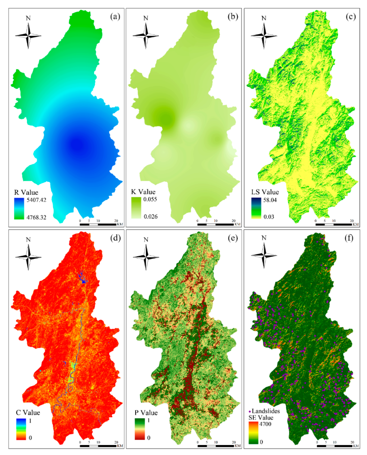
3.3. Modelling of Soil Erosion (SE) Intensity

SE is the process of soil destruction due to various external forces such as water power and wind power. The soil is eroded for a long time and can be regarded as the soil response under the integrated actions of rainfall, topographical factor, rock-soil properties, vegetation and human activities [57,58,59]. In this study, the Revised Universal Soil Loss Equation (RUSLE) model is used to calculate the SE modulus in the study area [60,61,62]. Then we can classify the SE modulus into five levels. According to the Technological Standard of Soil and Water Conservation (SL190-2007) [63], the very low level is of 0~5 t/ha, low level is of 5~25 t/ha, moderate level is of 25~50 t/ha, high level is of 50~80 t/ha and very high level is greater than80 t/ha. In general, the RUSLE is expressed as:
A = R × K × L × S × C × P
where A is the average annual SE amount per unit area (t/(ha·year); R and K respectively indicate the average rainfall erosivity ((MJ·mm)/(ha·h·year)) and the soil erodibility ((t·ha·h)/(MJ·ha·mm)); L and S respectively suggest the slope length and the slope steepness factors; C and P suggest the cover and management factor and the conservation practices factor, respectively. In general, all of the factors L , S , C and P are regarded as dimensionless.

3.4. Results of Soil Erosion Intensity Calculation

The calculation of SE intensity is mainly obtained through Equation (2) (Figure 4f). The daily rainfall data of 7 meteorological stations from 1998 to 2017 are used to obtain the rainfall erosivity R values of the whole research area through the kriging model ordinary with Gaussian semi-variational function [64] (Figure 4a). Soil erodibility factor K is obtained using the 1:4 million soil type data of Ningdu County in the second national soil survey and the K values of similar soil types near the study area [65,66] (Figure 4b). Topographic factor L S is obtained using the L S formula proposed by Y. Liu et al. [67] with DEM data (Figure 4c). The C value is acquired through widely used NDVI values (Figure 4d). The conservation practices factor P value is obtained by adopting manual interpretation of Landsat TM8 images and the current land use map of Ningdu County (Figure 4e). The above data are also checked through comparing with some other published papers [65,68,69,70] to ensure the reliability of this study.
The total amount of SE in Ningdu County obtained in this study is 3.832 million t, with a SE modulus of 940.37 t/km2, which can be considered as low SE. Studies have shown that the average SE modulus in the Poyang Lake watershed is approximately 1100 t/km2 [68], and that in Ganzhou City is 1386.66 t/km2 [70]. Due to the similar geographical environment characteristics between Ningdu County and the above study areas and the significant effects of various conservation practices carried out by the government in recent years, the SE modulus of Ningdu County has gradually decreased, and the prediction of SE distribution is reliable.

3.5. Landslide Susceptibility Prediction Model

3.5.1. Multilayer Perceptron (MLP)

The MLP is a feed-forward neural network typically used to address the binary classification problem of the complex mapping relationship between predisposing factors and landslide event occurrence in the LSP process. In this study, the MLP model with one input layer, multi-hidden layer and one output layer adopting the back propagation algorithm is proposed. First, the weight values of input and hidden layers are set randomly, and then the activation function in the hidden layer is used to address the sum of the product between the input layer and these weights. Then, the errors between the output value and the expected values are calculated. Finally, a minimum error result is obtained in the error back propagation iteration process. The MLP has the advantages of a good learning ability in the training stage and a realized optimal error in the automatic weight adjustment process. As a result, an accurate and stable prediction model can be constructed.

3.5.2. Logistic Regression (LR) Model

LR is a multivariate statistics method that has been widely used in the studies of landslide susceptibility all over the world [71]. The occurrence (set as 1) and/or non-occurrence (set as 0) probability of landslides can be calculated by LR model [72,73]. In this study, the LR model mainly uses the natural logarithm ratio (logit transformation) of landslide to non-landslide probability to construct a linear equation with each predisposing factor. The LR equation is expressed as:
L o g i t ( p ) = I n ( p 1 p ) = a 0 + a 1 x 1 + a 2 x 2 + a 3 x 3 + + a n x n
where p and 1 p respectively suggest the occurrence and non-occurrence probability of a landslide; x i   ( i = 1 , 2 , , n ) is the predisposing factor; a i   ( i = 1 , 2 , , n ) is coefficient value of x i   ( i = 1 , 2 , , n ) , and a i is positive, indicating that this factor has the positive effect on landslide occurrence; otherwise, it inhibits the landslide occurrence; a 0 suggests a regression constant value. Then the landslide susceptibility (named as occurrence probability) can be expressed as:
y = e a 0 + a 1 x 1 + a 2 x 2 + a 3 x 3 + + a n x n 1 + e a 0 + a 1 x 1 + a 2 x 2 + a 3 x 3 + + a n x n

3.5.3. Support Vector Machine (SVM)

SVM is often regarded as a classification system based on statistical learning theory [55,74]. This study adopts a set of linearly separable training vectors x i ( i = 1 , 2 , , n ) , including 10 predisposing factors and corresponding output classes y i = ± 1 and the maximum clearance of the n-dimensional hyper-plane to distinguish landslide susceptibility. Its expression is shown in Equation (5), and the constraint condition of correct classification is shown in Equation (6) with ω of hyper-plane norm and b of constant value.
1 2 ω 2
y i ( ( ω x i ) + b ) 1
Then, the Lagrange function is introduced to solve the problem of convex quadratic optimization, as shown in Equation (7) with λ i as a Lagrange multiplier. For linear inseparability, a slack variable is added to control the classification error. The constraint condition of correct classification is changed as shown in Equation (8).
L ( ω ) = 1 2 ω 2 i = 1 n λ i ( y i ( ( ω x i ) + b ) 1 )
y i ( ( ω x i ) + b ) 1 ξ i
ν ( 0 , 1 ) is introduced to consider misclassification, and the distance of the hyper-plane is shown in Equation (9). SVM possesses several kernel functions of polynomial and radial basis, and some studies have shown that the radial basis function kernel is more suitable for LSP [75].
L ( ω ) = 1 2 ω 2 1 ν n i = 1 n ξ i

3.5.4. C5.0 Decision Tree (C5.0 DT)

The C5.0 DT is an improved version of the C4.5 algorithm, which not only optimizes memory but also introduces the concept of entropy [76,77]. The C5.0 DT is an inverted tree composed of a root node, inner node and leaf node, and its purpose is to establish a set of optimal sequences to realize the classification of input variables. This algorithm segments the training data according to the variables providing the maximum information gain and then improves the classification accuracy and simplifies the model by deleting or pruning the unimportant leaves [78]. The information gain represents the importance of the variable, and its size also determines the priority selection order of the variable establishing the rule. The C5.0 DT can explain the establishment of sequence rules of the model more intuitively compared with the black-box models [79]. In addition, C5.0 DT adopts the adaptive boosting method. The fundamental idea is to construct the model in an orderly way, with the latter model building the next model based on the error classification samples of the former model, and so on. Finally, the weighted sum of each model is used to predict the whole model to improve the classification accuracy. The features of the data in the deepest node of the complete decision tree will lead to the over-fitting of the data. Therefore, the appropriate pruning of decision trees can reduce the inference rules with insignificant effects to limit the growth of trees and optimize the model.
The C5.0 DT modelling is built in this study. The output types of SE_C5.0 DT and C5.0 DT models are decision trees. The boosting method is used to improve the model accuracy with the number of experiments being 10. The accuracy of the model is estimated by cross-validation method with the folding numbers being 10. Meanwhile, the pruning degree of the expert model is selected to prune the decision tree in the model, and its value is set at 70 to avoid over-fitting of the model. In addition, the minimum number of records for each sub-branch in the decision tree is 15. An accurate model is obtained through the pruning degree and the minimum number of records of the sub-branch.

3.5.5. Statistically Significant Differences of Landslide Susceptibility Prediction (LSP) Models

To compare the statistically significant differences of LSP models before and after adding the SE factor, the Wilcoxon symbol rank test is used to conduct a non-parametric test on the two sets of LSIs calculated by the SE-based model and the single model. This method usually uses the Z value and P value to evaluate the significant differences between the two sets of LSIs. In general, there is a significant difference between the LSIs calculated by the SE-based models and single models if the Z value is outside the range of (−1.96, +1.96) and P value is less than 0.05 [80].

4. Results

The LSP modelling is carried out under both 30 m and 60 m resolutions using different models, aims to explore the effects of SE on landslide susceptibility. The MLP and LR models are built in the Statistical Product and Service Solutions (SPSS) 24.0 Software, meanwhile, the SVM and C5.0 DT models are built in the SPSS Modeler 18.0 Software.

4.1. LSP Results under 30 m Resolution

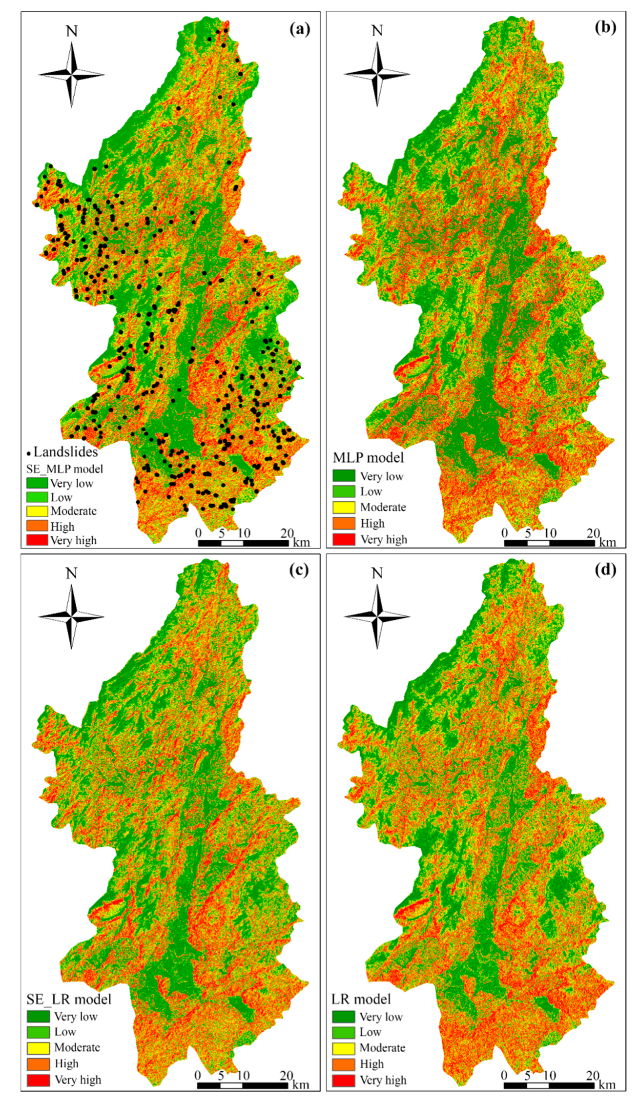
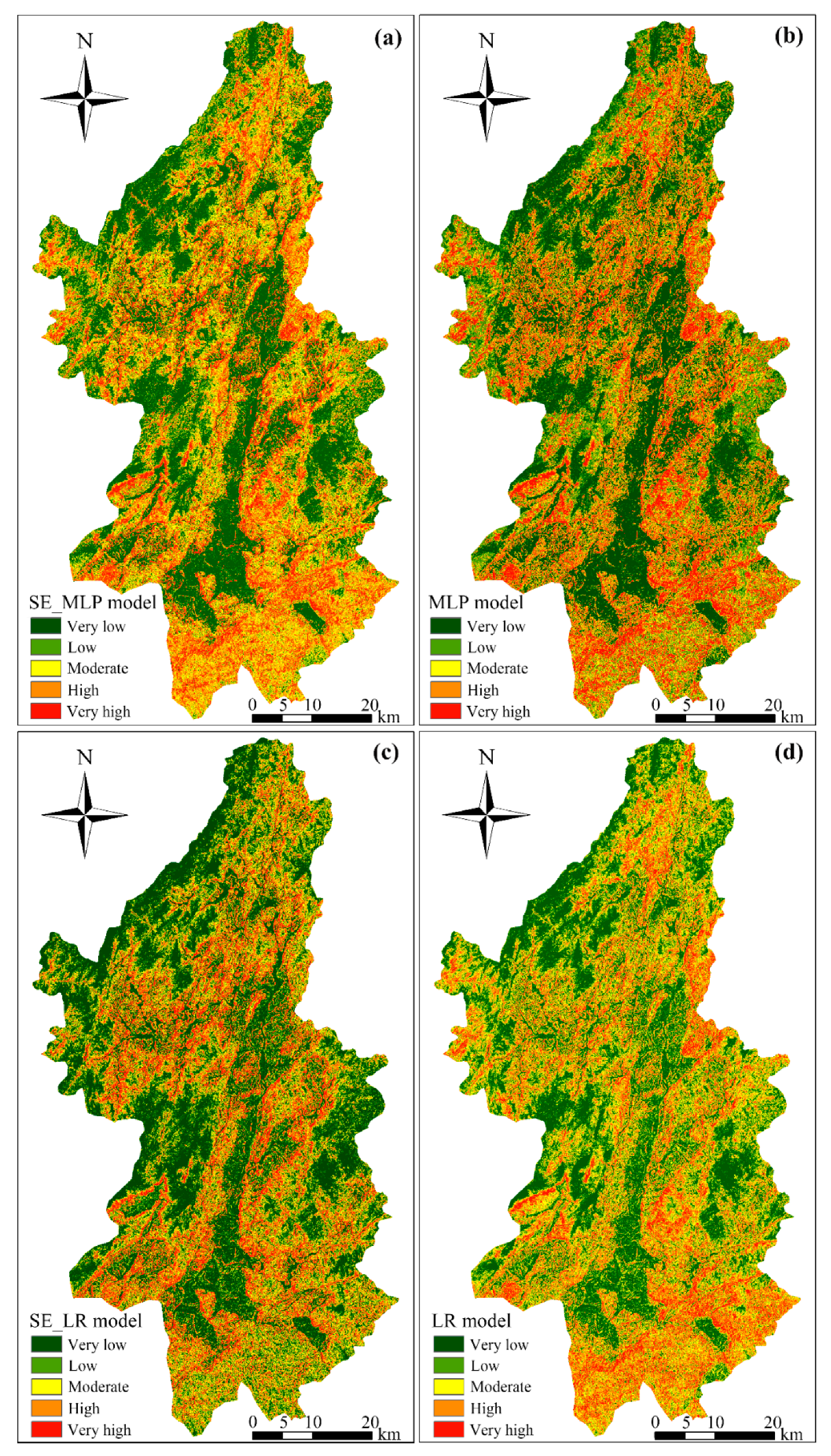
4.1.1. Landslide Susceptibility Maps (LSMs) of MLP Model

Based on the spatial database introduced in Section 3.3, the SE-based MLP model and single MLP model are adopted to carry out LSP in Ningdu County. Relevant parameters of both SE_MLP and MLP models are adjusted to construct the optimal models for LSP. The learning rate, momentum and iteration time in both models are 0.01, 0.25 and 500, respectively, and the number of hidden layers is set as two layers with the SoftMax activation function. The completely trained SE_MLP and MLP models are used to predict the LSI of each grid unit in Ningdu County. Then, two types of LSMs are produced under SE_MLP and MLP models by rasterizing the results obtained in ARCGIS 10.2. The LSMs in this study are reclassified into five LSLs: very low, low, moderate, high and very high-through Jenks natural break method [81] (Figure 5a,b). The area with very low LSL is maximum, while the low, moderate, high and very high LSLs are 30.93%, 17.79%, 18.26%, 19.14% and 13.88%, respectively, in the SE_MLP model.

4.1.2. LSMs of LR model

It is necessary to determine the independence of these predisposing factors to avoid information redundancy before modelling the SE_LR and LR. The correlation coefficient R of each predisposing factor is calculated with the correlation analysis tool in SPSS 24.0 software, which indicates that there are weak correlations among all predisposing factors. In addition, collinearity testing is also carried out for all input variables in this study, and the col-linearity between predisposing factors are identified adopting a variance inflation factor (VIF) and tolerance index (TOL), with VIF > 5 or TOL < 0.1 indicating the severity of col-linearity. As shown in Table 2, no multi-collinearity existed among these predisposing factors, with the maximum value of VIF being 1.592 and the minimum value of TOL being 0.628. Therefore, all 10 predisposing factors can be used as input variables of SE_LR and LR models.
The spatial dataset of the SE_LR model is imported into SPSS 24.0 software to acquire the regression coefficients ( β ), the standard error and significance of predisposing factors in the logistic regression equation. Table 2 shows that the significance of all predisposing factors is less than 0.05, indicating that all variables have statistical significance. The β values of all predisposing factors are positive, which indicates that all predisposing factors promote the occurrence of landslides. SE, elevation, lithology and NDBI with β values of 1.989, 1.589, 1.383 and 1.313, respectively, play the most important role in LSP modelling compared to other predisposing factors. In addition, the regression coefficients of elevation (1.581), slope (1.018), aspect (0.841), plan curvature (1.170), profile curvature (0.971), TWI (0.704), NDVI (0.506), NDBI (1.348) and lithology (1.316) and the regression intercept (–9.953) are determined for the single LR model. The obtained logistic regression coefficient and Equation (3) are used to obtain the LSIs in the study area, and the two types of LSMs are reclassified (Figure 5c,d). The results show that the very low, low, moderate, high and very high areas account for 25.57%, 23.46%, 20.38%, 17.87% and 12.72% of the total area, respectively, in the SE_LR model.

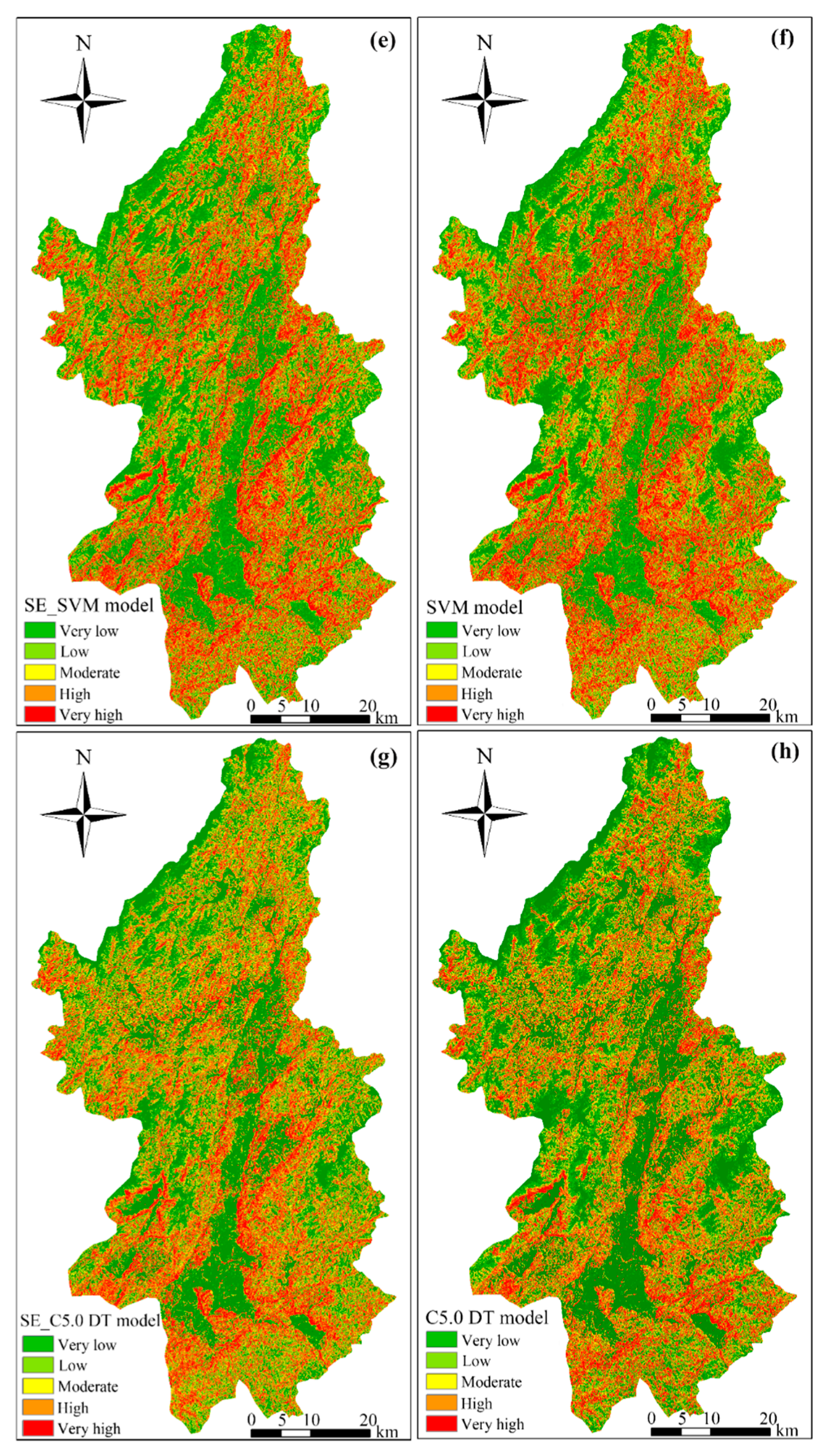
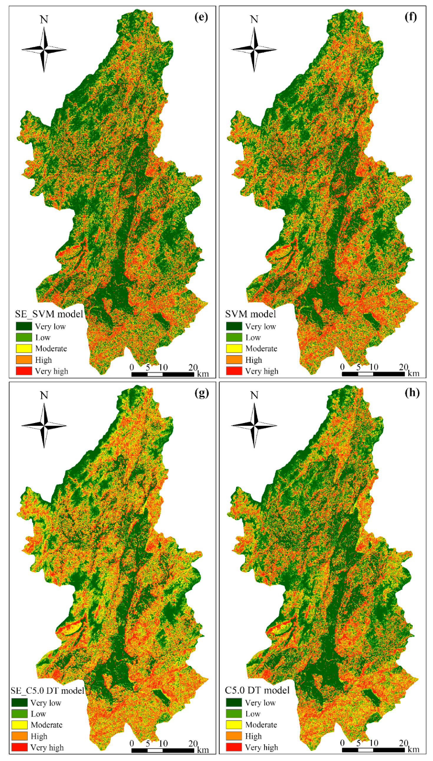
4.1.3. LSMs of SVM and C5.0 DT Models

In this study, the SE_SVM and SVM models are established with the kernel function of radial basis function (RBF). The stop standard, rule parameter (C), regression accuracy and kernel parameter (γ) of both models are 10−3, 9, 0.1 and 0.6, respectively. These trained models are used to predict the LSIs of all grid units (Figure 5e,f). The very high, high, moderate, low and very low areas, respectively, account for 20.15%, 14.43%, 13.57%, 22.67% and 29.18% of the total area for the SE_SVM model. The trained C5.0 DT model is used to obtain the LSIs of the study area and produces LSMs (Figure 5g,h). The very high, high, moderate, low and very low areas respectively account for 14.34%, 16.55%, 16.80%, 22.67% and 32.94% of the total area for the SE_C5.0 DT model.

4.2. LSP Results under 60 m Resolution

4.2.1. LSP Related Spatial Dataset Analysis

In order to explore the impact of SE on landslide susceptibility under different grid resolutions, the SE intensity in Ningdu County is calculated under 60 m resolution, then the other 9 conventional predisposing factors and the landslide inventory are also expressed with 60 m resolution. As a result, all 446 landslides are divided into 1748 landslide grid units which are set to 1, meanwhile, the same of 1748 non-landslide grid units are randomly selected in the study area and are set to 0. These 3496 landslide and non-landslide grid units are used as output variables of the SE-based and single models, and then are also randomly divided into a training and testing dataset with a ratio of 70/30%. The FR method is also used to calculate the non-linear correlations between landslide occurrences and predisposing factors.

4.2.2. LSMs Using SE-Based Model and Single Model

Firstly, the SE_MLP and single MLP models are built to produce the LSMs. The relatively optimal SE_MLP and single MLP models are constructed by adjusting the relevant parameters with the learning rate, momentum and iteration time in both models being set to 0.03, 0.5 and 500, respectively. The remaining parameters of the MLP model are the same as those under 30 m grid resolution. Then the trained SE-MLP and MLP models are adopted to predict the LSIs of grid units in Ningdu County and produce the LSMs (Figure 6a,b). The results show that the very low, low, moderate, high and very high susceptible areas respectively account for 29.49%, 15.42%, 21.29%, 18.59% and 15.21% of the total area in the SE_MLP model.
The parameters of the SE_LR model are shown in Table 3, suggesting that the SE, NDBI, slope, elevation and plan curvature factors play important roles in the processes of SE_LR model building. The LSMs are produced according to Equation (3) and are reclassified as shown in Figure 6c,d. Furthermore, the very low, low, moderate, high and very high susceptible areas respectively account for 35.31%, 19.74%, 18.61%, 15.67% and 10.67% of the total area for the SE_LR model.
For the use of SE_SVM and SVM models, The stop standard, rule parameter (C), regression accuracy and kernel parameter ( γ ) in both models are 10−3, 8, 0.1 and 0.7, respectively. The remaining SVM parameters are set to default values. Then, the trained SE_SVM and SVM models are used to predict LSIs and to produce LSMs (Figure 6e,f). Finally, the SE_C5.0 DT and C5.0 DT models are also used for LSP. In the adjustment processes of the SE_C5.0 DT and C5.0 DT models, the tree pruning degree is set to 60, and the minimum number of records for each sub-branch is set to 9. Then the LSMs produced by the trained SE_C5.0 DT and C5.0 DT models are shown in Figure 6g,h.

5. Discussion

In this paper, the importance of the SE factor in LSP modelling, the comparative studies between SE-based models and single models with no SE factor, and the statistical differences of LSP models under 30 m and 60 m resolutions are discussed.

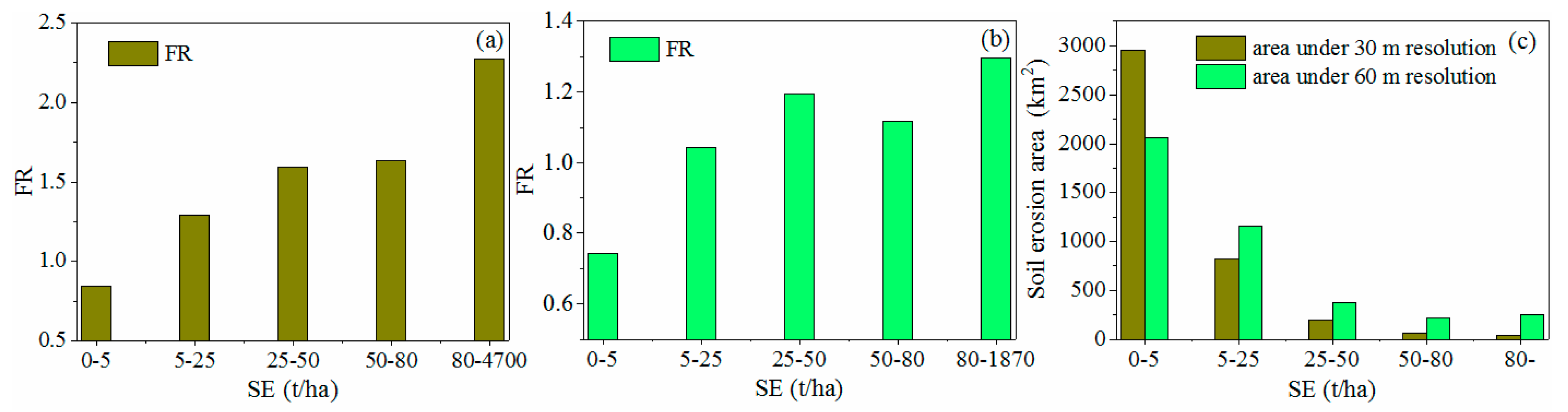
5.1. Frequency Ratio Analysis of SE Factor under Different Resolutions

The predisposing factors with different spatial resolutions have major influence on the results of soil erosion intensity and LSP. Taking the soil erosion prediction as example, the characteristic of soil erosion in different unit areas is one of difference, e.g., the maximum soil erosion modulus is about 4700 (t/ha) under 30 m resolution while 1870 (t/ha) under 60 m resolution. Similarly, the LSP results under 30 m and 60 m resolutions are also different from each other due to the changes of landslide grid units number and the corresponding predisposing factors. The purpose of using different resolutions is to avoid the effects of the prediction errors of landslide susceptibility and soil erosion amount on the research results, and to obtain more realistic and reliable influence rules of soil erosion factor on LSP.
Figure 7 indicates the relationship between landslide and SE classes and area distribution under 30 m and 60 m grid resolutions. Compared with the 60 m grid resolution, soil erosion under 30 m grid resolution has a stronger correlation with landslide events. The FR value is greater than 1 in the area with the high SE class and above, and it is 2.272 in the area with a very high class under 30 m grid resolution, where the FR is 2.68 times higher than that in the very low class. In addition, it is 1.295 in the area with a very high class under 60 m grid resolution. It is can be seen from Figure 7c that the area of SE with low level and above increase in 60 m grid resolution comparing with 30 m grid resolution.
However, the results in the two cases are similar in that soil erosion has a strong influence on the occurrence of landslide, which reflect how the frequency of landslides occurrence increases with the increase of soil erosion class (Figure 7a,b). The main reasons are that soil erosion reflects the soil loss amount under the coupling effects of rainfall, soil properties, topographic and land cover factors. Generally speaking, if a certain area has a more serious soil erosion condition, it indicates that there are worse environmental characteristics of brittle soil physical properties, complicated terrain, less land cover and/or sensitivity to heavy rainfall, which are more conducive to the occurrence of landslides [43]. Hence, soil erosion is one of the most important predisposing factors for the evolution of rainfall-induced shallow soil landslides. In this study, the FR values of the soil erosion factor embody the influence degrees of different classes of soil erosion intensity on the evolution of landslides, and the increase of FR value suggests that landslides are more likely to occur in areas with more serious soil erosion conditions. Therefore, FR values of the SE factor rise gradually with increasing SE intensity class.
The importance of each predisposing factor reflects the contribution of the predisposing factor to landslide occurrence. These four models are essentially non-linear predictors based on the determination processes of the weights of corresponding predisposing factors. The importance ranks of these predisposing factors are evaluated depending on the relative values of these weights according to the inherent classification attributes of these non-linear predictors. It can be seen from Figure 8a,b that the relative importance of predisposing factors in the SE_SVM model is different compared with other models, in which the relative importance of SE, NDBI and slope are 23%, 19% and 17%, respectively, while other factors are relatively small under 30 m resolution. The same phenomenon also happened under 60 m resolution. On the whole, SE, elevation, NDBI, and slope make great contributions in all models under both 30 m and 60 m grid resolutions. Specially, the SE factor has the largest contribution in each model, with a relative importance in SE_MLP, SE_LR, SE_SVM and SE_C5.0 of 21.6% (14.15%), 17.32% (16.81%), 23% (23.86%) and 13% (14.29%) under 30 m (60 m) grid resolutions, respectively.
Most of the landslides in Ningdu County belong to shallow soil landslides with characteristics of relatively loose soil, poor shear strength and sensitivity to rainfall. These unfavorable characteristics significantly improve the probability of landslide occurrence. At the same time, the SE can quantitatively reflect the processes of slope erosion and effect of sustained rainfall, and the product of soil erosion is the material source of slope accumulation layer [22,23]. Moreover, the FR values of landslides increase with the rise of SE level, suggesting that there is also a certain correlation between SE intensity and landslide occurrence [25]. Therefore, it is very necessary to consider the SE factor to improve the modelling accuracy of conventional LSP.

5.2. Accuracy Comparisons of SE-Based Models and Single Models under Different Resolutions

The evaluation of model performance is one of the key processes in successful LSP modelling, and the AUC is widely used to evaluate LSP performance [82,83]. The X-axis of the receiver operating characteristic (ROC) represents the proportion of non-landslides correctly classified as non-landslides, and the Y-axis represents the proportion of landslides correctly classified as landslides. The AUC can quantitatively reflect the model accuracy, and further analyses of the performance of the SE factor in each model as shown in Table 4, Figure 9 and Figure 10.
In terms of model performance, SE_MLP, SE_LR, SE_SVM and SE_C5.0 DT all have good predictive powers, with AUC values under 30 m (60 m) grid resolutions of 79.2% (76.2%), 78.3% (74.3%), 82.1% (82.4%) and 86.7% (79.7%), respectively. Meanwhile, the AUC values under 30 m and 60 m resolutions of single MLP, LR, SVM and C5.0 DT models with no SE factor are 76.2% (74%), 75.7% (72.3%), 79.6% (78.6%) and 84.8% (76.8%), respectively. The C5.0 DT model has the highest performance under 30 m resolution and the SVM model has the highest performance under 60 m resolution, while the LR model has the lowest prediction accuracy under both 30 m and 60 m resolutions. In addition, compared with the LSP accuracy under 60 m resolution, the LSP accuracy of the model increased as a whole under the 30 m resolution. However, the variation of SE on landslide susceptibility under different resolution are not great. The LSP accuracy of the SE-based models under 30 m resolution is 2~4% higher than that of the single models with no SE factor, and it is 2~5% under 60 m resolution. Moreover, the SE factor performs best in the MLP model under 30 m grid resolution, improving the accuracy by 3.94%, while it is in the SVM model with improving the accuracy by 4.83% under 60 m grid resolution. In a word, the 30 m grid resolution is more suitable for the prediction of landslide susceptibility. Furthermore, the effect of SE with different grid resolutions on landslide susceptibility is not significant, and SE can significantly improve the accuracy of the model under different supposed size.

5.3. Statistical Differences between SE-Based Models and Single Models

The statistically significant differences between the LSIs calculated by the SE-based models and single model are shown inTable 5, the LSIs under 30 m and 60 m resolutions between SE-based models and single models all show significant differences, indicating that the SE factor has a great influence on LSP results. Therefore, it is necessary to consider the SE factor as a new predisposing factor in LSP modelling processes.

6. Conclusions

This paper explores the effect of the SE factor on the LSP under different grid resolutions. The MLP, LR, SVM and C5.0 DT models are used to determine the importance ranking of the SE factor in each model and the performance of each model in LSP for Ningdu County, China. The LSP results of these SE-based models and single models with no SE factor are discussed.
(1)
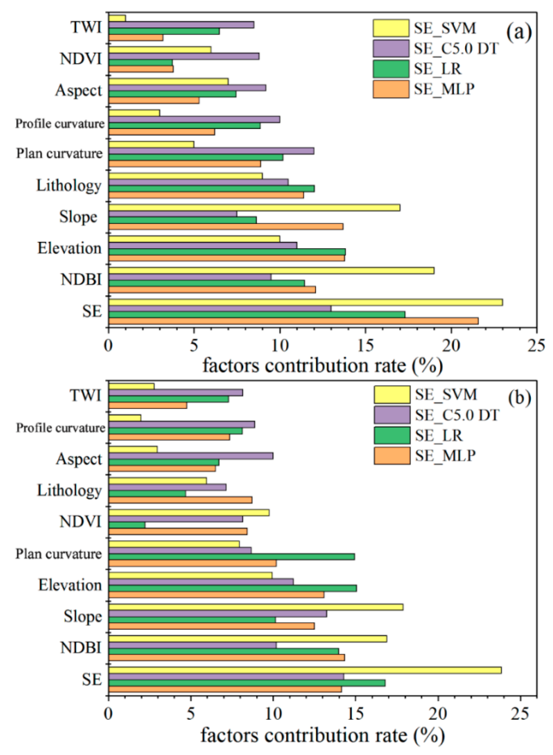
The FR analysis suggests that the FR value of SE gradually increases with the rise of soil erosion class, and the landslides are more inclined to the higher class soil erosion area. Furthermore, it can be concluded that the contribution of SE factor in all models is the largest under both 30 m and 60 m grid resolutions. That is to say, the SE factor plays the most important role in LSP modelling compared to the other traditional predisposing factors.
(2)
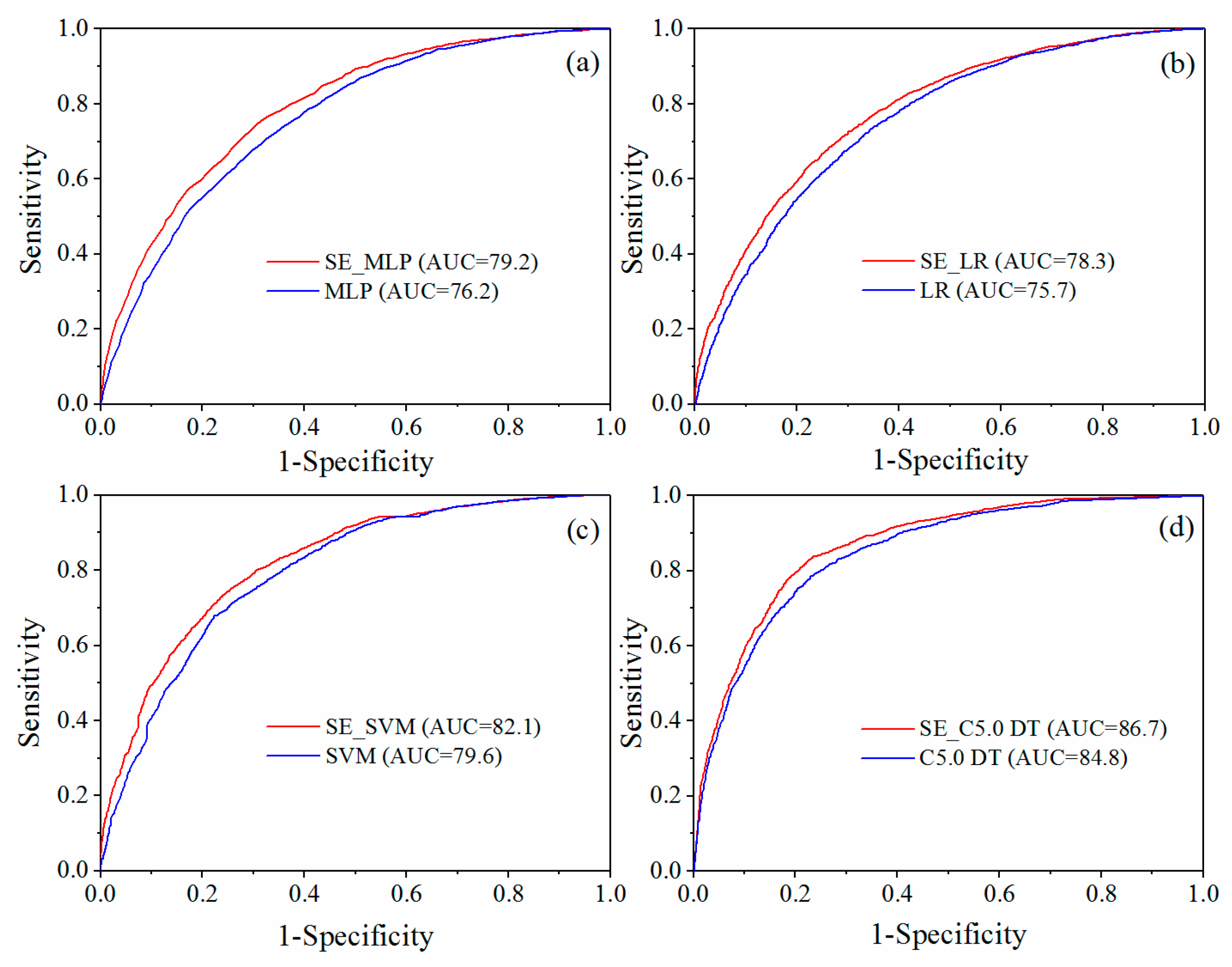
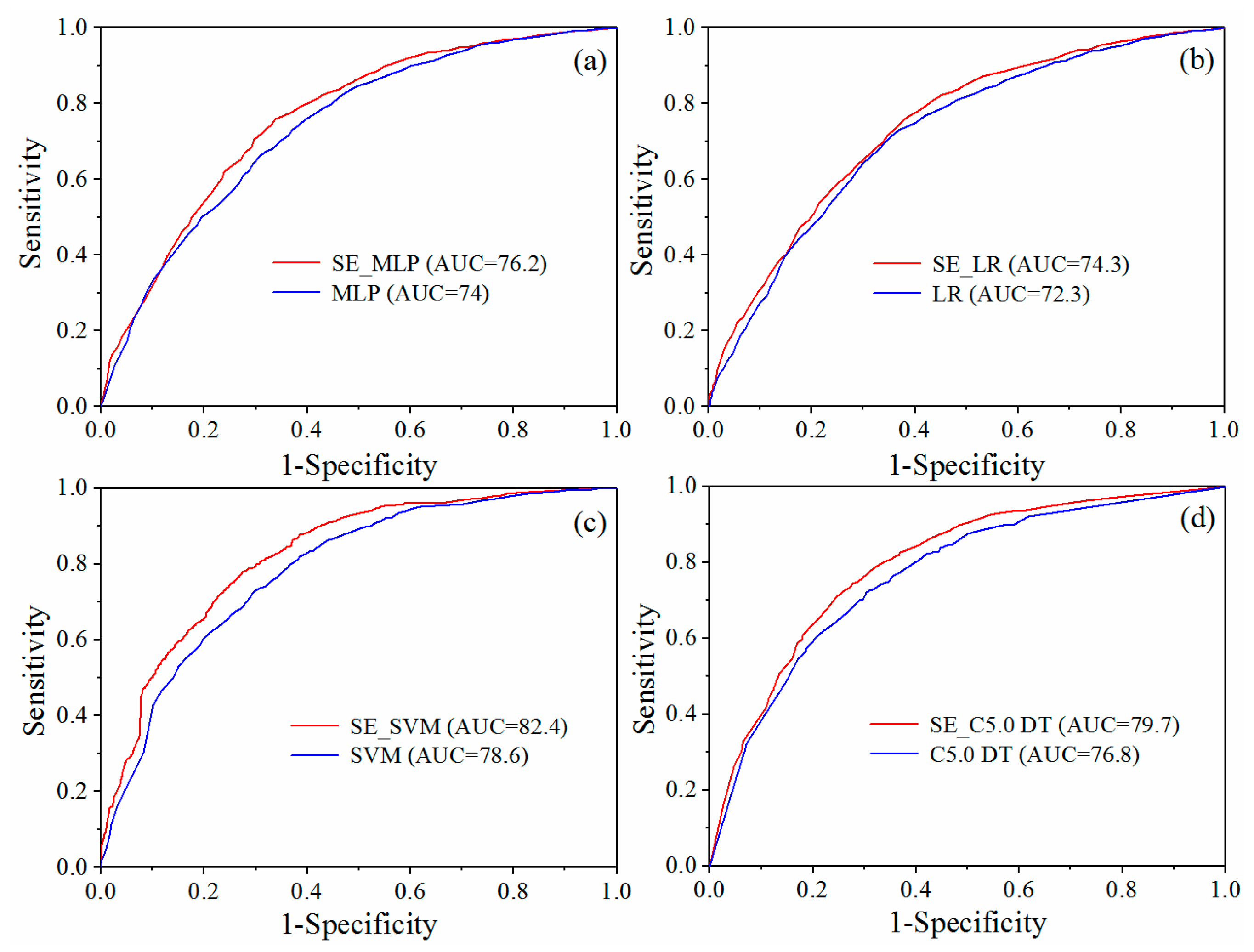
The comparison results show that the prediction accuracies of the four types of SE-based models are all higher than those of the single model under both 30 m and 60 m resolutions. In addition, the LSP accuracy under 30 m resolution is generally higher than that under 60 m resolution. Hence, it can be concluded that it is appropriate for LSP under 30 m resolution in Ningdu County, and the SE-based models are more appropriate for the LSP under both resolutions.
(3)
In general, under the conditions of 30 m and 60 m resolutions and the influences of SE factor, the C5.0 DT and SVM models show higher LSP performance than the MLP and LR models.
(4)
As a whole, the predicted distribution regularities of landslide susceptibility in Ningdu County can provide a theoretical basis for reducing local landslide risk and improving the control ability of geological disasters.

Author Contributions

Conceptualization: Faming Huang, Chi Yao and Jiawu Chen; methodology: Faming Huang and Jiawu Chen; software: Jiawu Chen and Zhilu Chang; validation: Jinsong Huang, and Zhen Du; formal analysis: Qinghui Jiang; investigation: Jiawu Chen and Zhilu Chang; resources: Faming Huang; data curation: Shu Li; writing—original draft preparation: Faming Huang, Jiawu Chen, Zhen Du, and Chi Yao; writing—review and editing: Faming Huang, Jinsong Huang, Qinghui Jiang, and Zhilu Chang; visualization: Jiawu Chen; supervision: Chi Yao; project administration: Chi Yao; funding acquisition: Faming Huang, Chi Yao, Qinghui Jiang, Jinsong Huang and Shu Li. All authors have read and agreed to the published version of the manuscript.

Funding

This research is funded by the National Key Research and Development Program (NO. 2017YFC1502505), the National Natural Science Foundation of China (No.41807285, 41762020, 51879127 and 51769014), the National Science Foundation of Jiangxi Province, China (20192BAB216034, 20192ACB2102, 20192ACB20020), the Postdoctoral Science Foundation of China (NO.2019M652287) and the Jiangxi Provincial Postdoctoral Science Foundation (NO. 2019KY08).

Conflicts of Interest

The authors declare no conflict of interest.

References

  1. Huang, F.; Wang, Y.; Dong, Z.; Wu, L.; Guo, Z.; Zhang, T. Regional landslide susceptibility mapping based on grey relational degree model. Earth Sci. 2019, 44, 664–676. [Google Scholar]
  2. Froude, M.J.; Petley, D.N. Global fatal landslide occurrence from 2004 to 2016. Nat. Hazards Earth Syst. Sci. 2018, 18, 2161–2181. [Google Scholar] [CrossRef] [Green Version]
  3. Dikshit, A.; Sarkar, R.; Pradhan, B.; Segoni, S.; Alamri, A.M. Rainfall induced landslide studies in indian himalayan region: A critical review. Appl. Sci. 2020, 10, 2466. [Google Scholar]
  4. Li, Y.; Huang, J.; Jiang, S.-H.; Huang, F.; Chang, Z. A web-based gps system for displacement monitoring and failure mechanism analysis of reservoir landslide. Sci. Rep. 2017, 7, 17171. [Google Scholar] [CrossRef] [Green Version]
  5. Liu, W.; Luo, X.; Huang, F.; Fu, M. Uncertainty of the soil–water characteristic curve and its effects on slope seepage and stability analysis under conditions of rainfall using the markov chain monte carlo method. Water 2017, 9, 758. [Google Scholar] [CrossRef] [Green Version]
  6. Chen, W.; Peng, J.; Hong, H.; Shahabi, H.; Pradhan, B.; Liu, J.; Zhu, A.X.; Pei, X.; Duan, Z. Landslide susceptibility modelling using gis-based machine learning techniques for chongren county, jiangxi province, china. Sci. Total Environ. 2018, 626, 1121–1135. [Google Scholar] [CrossRef]
  7. Dikshit, A.; Sarkar, R.; Pradhan, B.; Jena, R.; Drukpa, D.; Alamri, A.M. Temporal probability assessment and its use in landslide susceptibility mapping for eastern bhutan. Water 2020, 12, 267. [Google Scholar] [CrossRef] [Green Version]
  8. Cao, J.; Zhang, Z.; Wang, C.; Liu, J.; Zhang, L. Susceptibility assessment of landslides triggered by earthquakes in the western sichuan plateau. Catena 2019, 175, 63–76. [Google Scholar] [CrossRef]
  9. Razavizadeh, S.; Solaimani, K.; Massironi, M.; Kavian, A. Mapping landslide susceptibility with frequency ratio, statistical index, and weights of evidence models: A case study in northern iran. Environ. Earth Sci. 2017, 76, 499. [Google Scholar] [CrossRef]
  10. Ahmed, B.; Rahman, M.; Islam, R.; Sammonds, P.; Zhou, C.; Uddin, K.; Al-Hussaini, T.M. Developing a dynamic web-gis based landslide early warning system for the chittagong metropolitan area, bangladesh. Isprs Int. J. Geo-Inf. 2018, 7, 485. [Google Scholar] [CrossRef] [Green Version]
  11. Meena, S.R.; Ghorbanzadeh, O.; Blaschke, T. A comparative study of statistics-based landslide susceptibility models: A case study of the region affected by the gorkha earthquake in nepal. Isprs Int. J. Geo-Inf. 2019, 8, 94. [Google Scholar] [CrossRef] [Green Version]
  12. Ge, Y.; Chen, H.; Zhao, B.; Tang, H.; Zhong, P. A comparison of five methods in landslide susceptibility assessment: A case study from the 330-kv transmission line in gansu region, china. Environ. Earth Sci. 2018, 77, 662. [Google Scholar] [CrossRef]
  13. Carlà, T.; Raspini, F.; Intrieri, E.; Casagli, N. A simple method to help determine landslide susceptibility from spaceborne insar data: The montescaglioso case study. Environ. Earth Sci. 2016, 75, 1492. [Google Scholar] [CrossRef] [Green Version]
  14. Wu, X.; Niu, R.; Ren, F.; Peng, L. Landslide susceptibility mapping using rough sets and back-propagation neural networks in the three gorges, china. Environ. Earth Sci. 2013, 70, 1307–1318. [Google Scholar] [CrossRef]
  15. Huang, F.; Zhang, J.; Zhou, C.; Wang, Y.; Huang, J.; Zhu, L. A deep learning algorithm using a fully connected sparse autoencoder neural network for landslide susceptibility prediction. Landslides 2020, 17, 217–229. [Google Scholar] [CrossRef]
  16. Huang, F.; Yao, C.; Liu, W.; Li, Y.; Liu, X. Landslide susceptibility assessment in the nantian area of china: A comparison of frequency ratio model and support vector machine. Geomat. Nat. Hazards Risk 2018, 9, 919–938. [Google Scholar] [CrossRef] [Green Version]
  17. Huang, F.; Yin, K.; Huang, J.; Gui, L.; Wang, P. Landslide susceptibility mapping based on self-organizing-map network and extreme learning machine. Eng. Geol. 2017, 223, 11–22. [Google Scholar] [CrossRef]
  18. Arabameri, A.; Pradhan, B.; Lombardo, L. Comparative assessment using boosted regression trees, binary logistic regression, frequency ratio and numerical risk factor for gully erosion susceptibility modelling. Catena 2019, 183, 104223. [Google Scholar] [CrossRef]
  19. Guo, Z.; Yin, K.; Gui, L.; Liu, Q.; Huang, F.; Wang, T. Regional rainfall warning system for landslides with creep deformation in three gorges using a statistical black box model. Sci. Rep. 2019, 9, 8962. [Google Scholar] [CrossRef] [Green Version]
  20. Erener, A.; Mutlu, A.; Sebnem Düzgün, H. A comparative study for landslide susceptibility mapping using gis-based multi-criteria decision analysis (mcda), logistic regression (lr) and association rule mining (arm). Eng. Geol. 2016, 203, 45–55. [Google Scholar] [CrossRef]
  21. Duan, X.; Bing, L.; Gu, Z.; Li, R.; Feng, D. Quantifying soil erosion effects on soil productivity in the dry-hot valley, southwestern china. Environ. Earth Sci. 2016, 75, 1164. [Google Scholar] [CrossRef]
  22. Deng, H.; Wu, L.Z.; Huang, R.Q.; Guo, X.G.; He, Q. Formation of the siwanli ancient landslide in the dadu river, china. Landslides 2016, 14, 385–394. [Google Scholar] [CrossRef]
  23. Correa, S.W.; Mello, C.R.; Chou, S.C.; Curi, N.; Norton, L.D. Soil erosion risk associated with climate change at mantaro river basin, peruvian andes. Catena 2016, 147, 110–124. [Google Scholar] [CrossRef]
  24. Pradhan, B.; Chaudhari, A.; Adinarayana, J.; Buchroithner, M.F. Soil erosion assessment and its correlation with landslide events using remote sensing data and gis: A case study at penang island, malaysia. Environ. Monit. Assess. 2012, 184, 715–727. [Google Scholar] [CrossRef]
  25. Rozos, D.; Skilodimou, H.D.; Loupasakis, C.; Bathrellos, G.D. Application of the revised universal soil loss equation model on landslide prevention. An example from n. Euboea (evia) island, greece. Environ. Earth Sci. 2013, 70, 3255–3266. [Google Scholar] [CrossRef]
  26. Chen, Z.; Liang, S.; Ke, Y.; Yang, Z.; Zhao, H. Landslide susceptibility assessment using evidential belief function, certainty factor and frequency ratio model at baxie river basin, nw china. Geocarto Int. 2017, 34, 348–367. [Google Scholar] [CrossRef]
  27. Park, S.; Choi, C.; Kim, B.; Kim, J. Landslide susceptibility mapping using frequency ratio, analytic hierarchy process, logistic regression, and artificial neural network methods at the inje area, korea. Environ. Earth Sci. 2013, 68, 1443–1464. [Google Scholar] [CrossRef]
  28. Tsangaratos, P.; Ilia, I. Comparison of a logistic regression and naïve bayes classifier in landslide susceptibility assessments: The influence of models complexity and training dataset size. Catena 2016, 145, 164–179. [Google Scholar] [CrossRef]
  29. Zhang, K.; Wu, X.; Niu, R.; Yang, K.; Zhao, L. The assessment of landslide susceptibility mapping using random forest and decision tree methods in the three gorges reservoir area, china. Environ. Earth Sci. 2017, 76, 405. [Google Scholar] [CrossRef]
  30. Chang, Z.; Du, Z.; Zhang, F.; Huang, F.; Chen, J.; Li, W.; Guo, Z. Landslide susceptibility prediction based on remote sensing images and gis: Comparisons of supervised and unsupervised machine learning models. Remote Sens. 2020, 12, 502. [Google Scholar] [CrossRef] [Green Version]
  31. Song, Y.; Niu, R.; Xu, S.; Ye, R.; Peng, L.; Guo, T.; Li, S.; Chen, T. Landslide susceptibility mapping based on weighted gradient boosting decision tree in wanzhou section of the three gorges reservoir area (china). Isprs Int. J. Geo-Inf. 2019, 8, 4. [Google Scholar] [CrossRef] [Green Version]
  32. Ramesh, V.; Anbazhagan, S. Landslide susceptibility mapping along kolli hills ghat road section (india) using frequency ratio, relative effect and fuzzy logic models. Environ. Earth Sci. 2015, 73, 8009–8021. [Google Scholar] [CrossRef]
  33. Zhu, L.; Huang, L.; Fan, L.; Huang, J.; Huang, F.; Chen, J.; Zhang, Z.; Wang, Y. Landslide susceptibility prediction modeling based on remote sensing and a novel deep learning algorithm of a cascade-parallel recurrent neural network. Sensors 2020, 20, 1576. [Google Scholar] [CrossRef] [Green Version]
  34. Huang, F.; Wu, P.; Ziggah, Y. Gps monitoring landslide deformation signal processing using time-series model. Int. J. Signal Process. Image Process. Pattern Recognit. 2016, 9, 321–332. [Google Scholar] [CrossRef]
  35. Youssef, A.M.; Pourghasemi, H.R.; Pourtaghi, Z.S.; Alkatheeri, M.M. Landslide susceptibility mapping using random forest, boosted regression tree, classification and regression tree, and general linear models and comparison of their performance at wadi tayyah basin, asir region, saudi arabia. Landslides 2016, 13, 839–856. [Google Scholar] [CrossRef]
  36. Chen, W.; Wang, J.; Xie, X.; Hong, H.; Trung, N.V.; Bui, D.T.; Wang, G.; Li, X. Spatial prediction of landslide susceptibility using integrated frequency ratio with entropy and support vector machines by different kernel functions. Environ. Earth Sci. 2016, 75, 1344. [Google Scholar] [CrossRef]
  37. Huang, F.; Yin, K.; Zhang, G.; Zhou, C.; Zhang, J. Landslide groundwater level time series prediction based on phase space reconstruction and wavelet analysis-support vector machine optimized by pso algorithm. Earth Sci. -J. China Univ. Geosci. 2015, 40, 1254–1265. [Google Scholar]
  38. Huang, F.; Huang, J.; Jiang, S.; Zhou, C. Landslide displacement prediction based on multivariate chaotic model and extreme learning machine. Eng. Geol. 2017, 218, 173–186. [Google Scholar] [CrossRef]
  39. Zhu, X.; Xu, Q.; Tang, M.; Nie, W.; Ma, S.; Xu, Z. Comparison of two optimized machine learning models for predicting displacement of rainfall-induced landslide: A case study in sichuan province, china. Eng. Geol. 2017, 218, 213–222. [Google Scholar] [CrossRef]
  40. Li, D.; Huang, F.; Yan, L.; Cao, Z.; Chen, J.; Ye, Z. Landslide susceptibility prediction using particle-swarm-optimized multilayer perceptron: Comparisons with multilayer-perceptron-only, bp neural network, and information value models. Appl. Sci. 2019, 9, 3664. [Google Scholar] [CrossRef] [Green Version]
  41. Zhu, G.; Li, Y. Types and changes of chinese climate zones from 1961 to 2013 based on koppen climate classification. Arid Land Geogr. 2015, 38, 1121–1132. [Google Scholar]
  42. Hungr, O.; Leroueil, S.; Picarelli, L. The varnes classification of landslide types, an update. Landslides 2014, 11, 167–194. [Google Scholar] [CrossRef]
  43. Korte, D.M.; Shakoor, A. Landslide susceptibility and soil loss estimates for drift creek watershed, lincoln county, oregon. Environ. Eng. Geosci. 2019, 26, 167–184. [Google Scholar] [CrossRef]
  44. Cavazzi, S.; Corstanje, R.; Mayr, T.; Hannam, J.; Fealy, R. Are fine resolution digital elevation models always the best choice in digital soil mapping? Geoderma 2013, 195-196, 111–121. [Google Scholar] [CrossRef]
  45. Cama, M.; Conoscenti, C.; Lombardo, L.; Rotigliano, E. Exploring relationships between grid cell size and accuracy for debris-flow susceptibility models: A test in the giampilieri catchment (sicily, italy). Environ. Earth Sci. 2016, 75. [Google Scholar] [CrossRef]
  46. Huang, F.; Cao, Z.; Guo, J.; Jiang, S.-H.; Li, S.; Guo, Z. Comparisons of heuristic, general statistical and machine learning models for landslide susceptibility prediction and mapping. CATENA 2020, 191, 104580. [Google Scholar] [CrossRef]
  47. Sameen, M.I.; Sarkar, R.; Pradhan, B.; Drukpa, D.; Alamri, A.M.; Park, H.-J. Landslide spatial modelling using unsupervised factor optimisation and regularised greedy forests. Comput. Geosci. 2020, 134. [Google Scholar] [CrossRef]
  48. Chen, W.; Pourghasemi, H.R.; Panahi, M.; Kornejady, A.; Wang, J.; Xie, X.; Cao, S. Spatial prediction of landslide susceptibility using an adaptive neuro-fuzzy inference system combined with frequency ratio, generalized additive model, and support vector machine techniques. Geomorphology 2017, 297, 69–85. [Google Scholar] [CrossRef]
  49. Huang, F.; Chen, L.; Yin, K.; Huang, J.; Gui, L. Object-oriented change detection and damage assessment using high-resolution remote sensing images, tangjiao landslide, three gorges reservoir, china. Environ. Earth Sci. 2018, 77, 183. [Google Scholar] [CrossRef]
  50. Huang, F.; Huang, J.; Jiang, S.-H.; Zhou, C. Prediction of groundwater levels using evidence of chaos and support vector machine. J. Hydroinform. 2017, 19, 586–606. [Google Scholar] [CrossRef] [Green Version]
  51. Liu, W.; Luo, X.; Huang, F.; Fu, M. Prediction of soil water retention curve using bayesian updating from limited measurement data. Appl. Math. Model. 2019, 76, 380–395. [Google Scholar] [CrossRef]
  52. Kritikos, T.; Davies, T. Assessment of rainfall-generated shallow landslide/debris-flow susceptibility and runout using a gis-based approach: Application to western southern alps of new zealand. Landslides 2015, 12, 1051–1075. [Google Scholar] [CrossRef]
  53. Su, C.; Wang, L.; Wang, X.; Huang, Z.; Zhang, X. Mapping of rainfall-induced landslide susceptibility in wencheng, china, using support vector machine. Nat. Hazards 2015, 76, 1759–1779. [Google Scholar] [CrossRef]
  54. Huang, F.; Luo, X.; Liu, W. Stability analysis of hydrodynamic pressure landslides with different permeability coefficients affected by reservoir water level fluctuations and rainstorms. Water 2017, 9, 450. [Google Scholar] [CrossRef] [Green Version]
  55. Bui, D.T.; Tuan, T.A.; Klempe, H.; Pradhan, B.; Revhaug, I. Spatial prediction models for shallow landslide hazards: A comparative assessment of the efficacy of support vector machines, artificial neural networks, kernel logistic regression, and logistic model tree. Landslides 2016, 13, 361–378. [Google Scholar]
  56. Ahmed, B.; Dewan, A. Application of bivariate and multivariate statistical techniques in landslide susceptibility modeling in chittagong city corporation, bangladesh. Remote Sens. 2017, 9, 304. [Google Scholar] [CrossRef] [Green Version]
  57. Karan, S.K.; Ghosh, S.; Samadder, S.R. Identification of spatially distributed hotspots for soil loss and erosion potential in mining areas of upper damodar basin - india. Catena 2019, 182, 9. [Google Scholar] [CrossRef]
  58. Kinnell, P.I.A. Determining soil erodibilities for the usle-mm rainfall erosion model. Catena 2018, 163, 424–426. [Google Scholar] [CrossRef]
  59. Mhaske, S.N.; Pathak, K.; Basak, A. A comprehensive design of rainfall simulator for the assessment of soil erosion in the laboratory. Catena 2019, 172, 408–420. [Google Scholar] [CrossRef]
  60. Ganasri, B.P.; Ramesh, H. Assessment of soil erosion by rusle model using remote sensing and gis—A case study of nethravathi basin. Geosci. Front. 2016, 7, 953–961. [Google Scholar] [CrossRef] [Green Version]
  61. Zhang, H.D.; Zhang, R.H.; Qi, F.; Liu, X.; Niu, Y.; Fan, Z.F.; Zhang, Q.H.; Li, J.Z.; Yuan, L.; Song, Y.Y.; et al. The csle model based soil erosion prediction: Comparisons of sampling density and extrapolation method at the county level. Catena 2018, 165, 465–472. [Google Scholar] [CrossRef]
  62. Vanacker, V.; Ameijeiras-Marino, Y.; Schoonejans, J.; Cornelis, J.T.; Minella, J.P.G.; Lamouline, F.; Vermeire, M.L.; Campforts, B.; Robinet, J.; Van de Broek, M.; et al. Land use impacts on soil erosion and rejuvenation in southern brazil. Catena 2019, 178, 256–266. [Google Scholar] [CrossRef] [Green Version]
  63. Xue, J.; Lyu, D.; Wang, D.; Wang, Y.; Yin, D.; Zhao, Z.; Mu, Z. Assessment of soil erosion dynamics using the gis-based rusle model: A case study of wangjiagou watershed from the three gorges reservoir region, southwestern china. Water 2018, 10, 1817. [Google Scholar] [CrossRef] [Green Version]
  64. Pesquer, L.; Cortés, A.; Pons, X. Parallel ordinary kriging interpolation incorporating automatic variogram fitting. Comput. Geosci. 2011, 37, 464–473. [Google Scholar] [CrossRef]
  65. Yuan, L.; Yang, G.; Zhang, Q.; Li, H. Soil erosion assessment of the poyang lake basin, china: Using usle, gis and remote sensing. J. Remote Sens. GIS 2016, 5, 2. [Google Scholar]
  66. Zhong, R.-l.; Xiao, X.; Zhang, P.-c.; Cen, Y. Research on spatial variability statement methods of soil anti-erodibility in jiangxi province. J. Yangtze River Sci. Res. Inst. 2010, 27, 13–18. [Google Scholar]
  67. Liu, B.; Nearing, M.; Risse, L. Slope gradient effects on soil loss for steep slopes. Trans. ASAE 1994, 37, 1835–1840. [Google Scholar] [CrossRef]
  68. Lu, J.; Chen, X.; Li, H.; Liu, H.; Xiao, J.; Yin, J. Soil erosion changes based on gis/rs and usle in poyang lake basin. Trans. Chin. Soc. Agric. Eng. 2011, 27, 337–344. [Google Scholar]
  69. Shi, D.; Shi, X.; Li, D. Study on dynamic monitoring of soil erosion using remote sensing technique. Acta Pedol. Sin. 1996, 33, 48–58. [Google Scholar]
  70. Li, H.; Yang, L.; Lei, j. Soil erosion analysis in red soil hilly region by using hj-ccd: A case study in ganzhou. Remote sensing information. Remote Sens. Inf. 2016, 31, 122–129. [Google Scholar]
  71. Pourghasemi, H.R.; Teimoori Yansari, Z.; Panagos, P.; Pradhan, B. Analysis and evaluation of landslide susceptibility: A review on articles published during 2005–2016 (periods of 2005–2012 and 2013–2016). Arab. J. Geosci. 2018, 11. [Google Scholar] [CrossRef]
  72. Hong, H.; Pourghasemi, H.R.; Pourtaghi, Z.S. Landslide susceptibility assessment in lianhua county (china): A comparison between a random forest data mining technique and bivariate and multivariate statistical models. Geomorphology 2016, 259, 105–118. [Google Scholar] [CrossRef]
  73. Sevgen, E.; Kocaman, S.; Nefeslioglu, H.A.; Gokceoglu, C. A novel performance assessment approach using photogrammetric techniques for landslide susceptibility mapping with logistic regression, ann and random forest. Sensors 2019, 19, 3940. [Google Scholar] [CrossRef] [PubMed] [Green Version]
  74. Tien Bui, D.; Shahabi, H.; Shirzadi, A.; Chapi, K.; Alizadeh, M.; Chen, W.; Mohammadi, A.; Ahmad, B.B.; Panahi, M.; Hong, H.; et al. Landslide detection and susceptibility mapping by airsar data using support vector machine and index of entropy models in cameron highlands, malaysia. Remote Sens. 2018, 10, 1527. [Google Scholar] [CrossRef] [Green Version]
  75. Xu, C.; Dai, F.; Xu, X.; Lee, Y.H. Gis-based support vector machine modeling of earthquake-triggered landslide susceptibility in the jianjiang river watershed, china. Geomorphology 2012, 145, 70–80. [Google Scholar] [CrossRef]
  76. Saito, H.; Nakayama, D.; Matsuyama, H. Comparison of landslide susceptibility based on a decision-tree model and actual landslide occurrence: The akaishi mountains, japan. Geomorphology 2009, 109, 108–121. [Google Scholar] [CrossRef]
  77. Tseng, C.J.; Lu, C.J.; Chang, C.C.; Chen, G.D.; Cheewakriangkrai, C. Integration of data mining classification techniques and ensemble learning to identify risk factors and diagnose ovarian cancer recurrence. Artif. Intell. Med. 2017, 78, 47–54. [Google Scholar] [CrossRef]
  78. Golkarian, A.; Naghibi, S.A.; Kalantar, B.; Pradhan, B. Groundwater potential mapping using c5.0, random forest, and multivariate adaptive regression spline models in gis. Environ. Monit. Assess. 2018, 190, 149. [Google Scholar] [CrossRef]
  79. Wu, X.; Ren, F.; Niu, R. Landslide susceptibility assessment using object mapping units, decision tree, and support vector machine models in the three gorges of china. Environ. Earth Sci. 2013, 71, 4725–4738. [Google Scholar] [CrossRef]
  80. Chen, W.; Xie, X.; Wang, J.; Pradhan, B.; Hong, H.; Bui, D.T.; Duan, Z.; Ma, J. A comparative study of logistic model tree, random forest, and classification and regression tree models for spatial prediction of landslide susceptibility. Catena 2017, 151, 147–160. [Google Scholar] [CrossRef] [Green Version]
  81. Cantarino, I.; Carrion, M.A.; Goerlich, F.; Martinez Ibañez, V. A roc analysis-based classification method for landslide susceptibility maps. Landslides 2018, 16, 265–282. [Google Scholar] [CrossRef]
  82. Hong, H.; Panahi, M.; Shirzadi, A.; Ma, T.; Liu, J.; Zhu, A.X.; Chen, W.; Kougias, I.; Kazakis, N. Flood susceptibility assessment in hengfeng area coupling adaptive neuro-fuzzy inference system with genetic algorithm and differential evolution. Sci. Total Environ. 2018, 621, 1124–1141. [Google Scholar] [CrossRef] [PubMed]
  83. Reichenbach, P.; Rossi, M.; Malamud, B.D.; Mihir, M.; Guzzetti, F. A review of statistically-based landslide susceptibility models. Earth-Sci. Rev. 2018, 180, 60–91. [Google Scholar] [CrossRef]
Figure 1. Location of the study area and landslide inventory.
Ijgi 09 00377 g001
Figure 2. Predisposing factors under 30 m resolution: (a) elevation; (b) slope; (c) aspect; (d) plan curvature; (e) profile curvature; (f) topographic wetness index (TWI); (g) normalized difference vegetation index (NDVI); (h) normalized difference built-up index (NDBI); (i) lithology.
Ijgi 09 00377 g002
Figure 3. Flowchart of this study.
Ijgi 09 00377 g003
Figure 4. SE values and related factors with 30 m resolutions: (a) R value; (b) K value; (c) LS value; (d) C value; (e) P value; (f) SE value.
Ijgi 09 00377 g004
Figure 5. Landslide susceptibility maps with 30 m grid resolutions: (a) SE_MLP model; (b) MLP model; (c) SE_LR model; (d) LR model; (e) SE_SVM model; (f) SVM model; (g) SE_C5.0 DT model; (h) C5.0 DT model.
Ijgi 09 00377 g005aIjgi 09 00377 g005b
Figure 6. LSMs of each model with 60 m grid resolutions: (a) SE_MLP model; (b) MLP model; (c) SE_LR model; (d) LR model; (e) SE_SVM model; (f) SVM model; (g) SE_C 5.0 DT model; (h) C 5.0 DT model.
Ijgi 09 00377 g006aIjgi 09 00377 g006b
Figure 7. FR values between SE and landslides with resolutions of 30 m (a), 60 m (b) and areas distribution (c) 5.2. Importance Analysis of Soil Erosion in LSP.
Ijgi 09 00377 g007
Figure 8. Relative importance of landslide factors in different models with 30 m (a) and 60 m (b) resolutions.
Ijgi 09 00377 g008
Figure 9. AUC value of each model with grid resolutions of 30 m: AUC values of SE_MLP and MLP models (a); AUC values of SE_LR and LR models (b); AUC values of SE_SVM and SVM models (c); AUC values of SE_C5.0 DT and C5.0 DT models (d).
Ijgi 09 00377 g009
Figure 10. AUC value of each model with grid resolutions of 60 m: AUC values of SE_MLP and MLP models (a); AUC values of SE_LR and LR models (b); AUC values of SE_SVM and SVM models (c); AUC values of SE_C5.0 DT and C5.0 DT models (d).
Ijgi 09 00377 g010
Table 1. Classifications of landslide predisposing factors with 30 m resolution.
Predisposing FactorsClassification
Elevation (m)[155,244); [244,322); [322,411); [411,509); [509,618); [618,751); [751,938); [938,1411)
Slope (°)[0.00,3.53); [3.53,7.27); [7.27,11.23); [11.23,15.18); [15.18,19.33); [19.33,24.12); [24.12,30.35); [30.35,53.02)
AspectFlat; North; Northeast; East; Southeast; South; Southwest; West; Northwest
Plan curvature[0.00,9.91); [9.91,18.22); [18.22,27.48); [27.48,37.39); [37.39,47.94); [47.94,58.81); [58.81,70.64); [70.64,81.50)
Profile curvature[0.00,1.53); [1.53,3.05); [3.05,4.71); [4.71,6.48); [6.48,8.52); [8.52,11.06); [11.06,14.75); [14.75,32.44)
TWI[2.79,5.65); [5.65,7.24); [7.24,9.15); [9.15,11.69); [11.69,15.34); [15.34,24.39); [24.39,43.28)
NDVI[−0.187,0.025); [0.025,0.131); [0.131,0.196); [0.196,0.243); [0.243,0.282); [0.282,0.321); [0.321,0.362); [0.362,0.516)
NDBI[−0.502,−0.379); [−0.379,−0.337); [−0.337,−0.292); [−0.292,−0.244); [−0.244,−0.191); [−0.191,−0.135); [−0.135,−0.067); [−0.067,0.455)
Lithologymetamorphic rock; magmatic rock; clastic rock; carbonate rock; water body
SE (t/ha)[0,5); [5,25); [25,50); [50,80); [80,4700.75)
Table 2. Parametric statistics in the soil erosion–logistic regression (SE_LR) model with 30 m grid resolutions.
VariablesβStandard ErrorSIGCollinear Statistics
Variance Inflation Factor Tolerance
Elevation1.5890.1150.0001.1020.907
Slope0.9930.0600.0001.1720.853
Aspect0.8570.1440.0001.0420.960
Plan curvature1.0200.1670.0001.0830.924
Profile curvature1.1700.0860.0001.1170.895
Lithology1.3830.1050.0001.0770.928
NDBI1.3130.1060.0001.5750.635
NDVI0.4290.1550.0061.5920.628
TWI0.7440.1360.0001.1000.909
SE1.9890.1120.0001.0180.982
constant-11.9690.3980.000--
Table 3. Parametric statistics in the SE_LR model with 60 m grid resolutions.
VariablesβStandard ErrorSIGCollinear Statistics
Variance Inflation Factor Tolerance
Elevation1.3820.1660.0001.1910.839
Slope0.930.0830.0001.1360.880
Aspect0.6170.2150.0031.0330.968
Plan curvature1.3720.1560.0001.0840.922
Profile curvature0.7480.2120.0001.1320.883
Lithology0.4310.1510.0001.0890.918
NDBI1.2830.140.0001.7960.557
NDVI0.2050.2080.0001.9100.524
TWI0.6690.1360.0011.0450.957
SE1.5430.2070.0001.0040.998
constant-9.1270.5110.000--
Table 4. Performance of each LSP model with resolutions of 30 m and 60 m.
Gird ResolutionModelsAUC with SE (%)AUC with No SE (%)Improvement (%)
30 mMLP79.276.23.94
LR78.375.73.43
SVM82.179.63.14
C5.0 DT86.784.82.24
60 mMLP76.274.02.97
LR74.372.32.77
SVM82.478.64.83
C5.0 DT79.776.83.78
Table 5. Comparison of the results before and after adding SE in models with resolutions of 30 m (60 m).
ResolutionParameterMLPLRSVMC5.0 DT
30 mZ−3.323−2.879−5.871−2.358
P0.0010.0040.0000.018
60 mZ−6.703−2.223−3.176−6.953
P0.0000.0260.0010.000

