Landslide Susceptibility Prediction Based on Remote Sensing Images and GIS: Comparisons of Supervised and Unsupervised Machine Learning Models

Abstract

Landslide susceptibility prediction (LSP) has been widely and effectively implemented by machine learning (ML) models based on remote sensing (RS) images and Geographic Information System (GIS). However, comparisons of the applications of ML models for LSP from the perspectives of supervised machine learning (SML) and unsupervised machine learning (USML) have not been explored. Hence, this study aims to compare the LSP performance of these SML and USML models, thus further to explore the advantages and disadvantages of these ML models and to realize a more accurate and reliable LSP result. Two representative SML models (support vector machine (SVM) and CHi-squared Automatic Interaction Detection (CHAID)) and two representative USML models (K-means and Kohonen models) are respectively used to scientifically predict the landslide susceptibility indexes, and then these prediction results are discussed. Ningdu County with 446 recorded landslides obtained through field investigations is introduced as case study. A total of 12 conditioning factors are obtained through procession of Landsat TM 8 images and high-resolution aerial images, topographical and hydrological spatial analysis of Digital Elevation Modeling in GIS software, and government reports. The area value under the curve of receiver operating features (AUC) is applied for evaluating the prediction accuracy of SML models, and the frequency ratio (FR) accuracy is then introduced to compare the remarkable prediction performance differences between SML and USML models. Overall, the receiver operation curve (ROC) results show that the AUC of the SVM is 0.892 and is slightly greater than the AUC of the CHAID model (0.872). The FR accuracy results show that the SVM model has the highest accuracy for LSP (77.80%), followed by the CHAID model (74.50%), the Kohonen model (72.8%) and the K-means model (69.7%), which indicates that the SML models can reach considerably better prediction capability than the USML models. It can be concluded that selecting recorded landslides as prior knowledge to train and test the LSP models is the key reason for the higher prediction accuracy of the SML models, while the lack of a priori knowledge and target guidance is an important reason for the low LSP accuracy of the USML models. Nevertheless, the USML models can also be used to implement LSP due to their advantages of efficient modeling processes, dimensionality reduction and strong scalability.

1. Introduction

Landslides are considered as one type of the most serious natural disasters around the world. The safety of local residents and property is frequently destroyed by some triggered landslides [1,2,3]. Accurately predicting the potential location of landslide occurrence in advance can significantly reduce losses. The landslide susceptibility prediction (LSP) is considered as an effective tool to determine the landslide occurrence possibility in a certain study area. LSP involves comprehensive evaluation of the landslide-inducing conditioning factors and the characteristics of recorded landslides, which are mainly extracted from the remote sensing (RS) images and spatial analysis of Geographic Information System (GIS) [4].

LSP is one of the most important research bases of landslide risk prediction. To obtain reasonable LSP results, it is crucial to select appropriate prediction models that accept the landslide-relevant thematic information. Conventionally, the LSP models can be divided into these types as probability analysis models [5], heuristic models [1], deterministic models [6] and statistical models [7]. On the whole, these types of models contribute to the development of LSP and are regarded as effective technologies. Many attentions have been paid to overcome the limitations of the high subjectivity in determining the parameters of probability analysis and heuristic models [8,9,10,11]. At the same time, aiming at the difficulty in acquiring the reliable parameters of deterministic models, many researches have tried their best to improve the accuracy of deterministic models by incorporating advanced soil properties [12,13,14]. In particular, in recent years, many excellent machine learning (ML) models that can efficiently fit and predict the nonlinear correlations between landslides and related conditioning factors, have been proposed to address the drawbacks of the conventional statistical models. Related literature shows that the ML models have been more and more popularly used for LSP [15,16,17,18].

In general, according to whether labeled data are used as the prior knowledge in the modeling process, ML models can be classified as: supervised machine learning (SML) using a priori knowledge and unsupervised machine learning models (USML) without prior knowledge. In previous LSP studies, the frequently used SML models include most artificial neural networks [19,20], support vector machines [21,22,23], decision tree methods [24,25,26], random forest [27,28], logistic regression [29,30,31], fuzzy mathematical theory [32], etc. These types of models perform very well for LSP in many research areas due to their advantages in supervised data mining [33]. The frequently used USML models include K-means model [34,35], self-organization mapping (SOM) model [15,36], principal component analysis [37,38], hierarchical cluster analysis [39], and so on. These models have also been widely used in LSP because the modeling process is simple [40].

SML and USML are the most popular classification criteria of ML models. It is important to adopt different classes of models to evaluate and compare LSP results, and many studies have focused on this issue [41,42], because no agreement is reached about which type of model is the most appropriate one for LSP. Therefore, the work of exploring the comparisons of SML and USML models for LSP is very meaningful. Unfortunately, the literature shows that comparison studies about LSP performance and results implemented by the SML and USML models have rarely been reported.

To summarize, the goal of this paper thus is to assess and compare the LSP results from the perspectives of SML and USML models based on RS and GIS platforms, and further to choose the most appropriate to generate accurate and reliable LSP. Two typical SML models (support vector machine (SVM) and CHi-squared Automatic Interaction Detection (CHAID), and two other typical USML models (K-means and Kohonen models) are applied to implement LSP. Then, the applications and accuracies of SML and USML for LSP are discussed and analyzed.

2. Materials and Methods

2.1. Materials

The materials include the study area description, landslide inventory information, and the description of related conditioning factors.

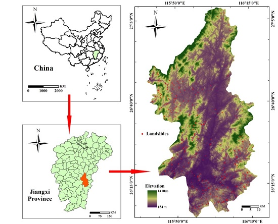
2.1.1. Study Area and Landslide Inventory Information

Ningdu County of Jiangxi Province, in China is chosen as research area since it is seriously affected by landslide disasters. Ningdu County locates in longitudes 26°05′18″–27°08′13″N and latitudes 115°40′20″–116°17′15″E (Figure 1). The area of Ningdu County is about 4053.16 km². The study area has a sub-tropical monsoon climate with annual average rainfall ranging from 1500 to 1700 mm. The total rainfall amounts in the north and east zones being larger than those in the south and west zones.

The landslide inventory information in Ningdu County are measured through Global Position System (GPS) [43] field investigations (Figure 1). Based on field investigation results and landslide inventory, there are a total of 446 recorded landslides, which are small shallow landslides with areas ranging from 759.17 m² to 44,368.0 m² and an average area about 10,000 m². The landslide masses are mainly composed of Quaternary alluvium, and the failure modes are mainly retrogressive sliding. Furthermore, it can be found that the main trigger factors of landslides occurrence are continuous heavy rainfall and human engineering activities.

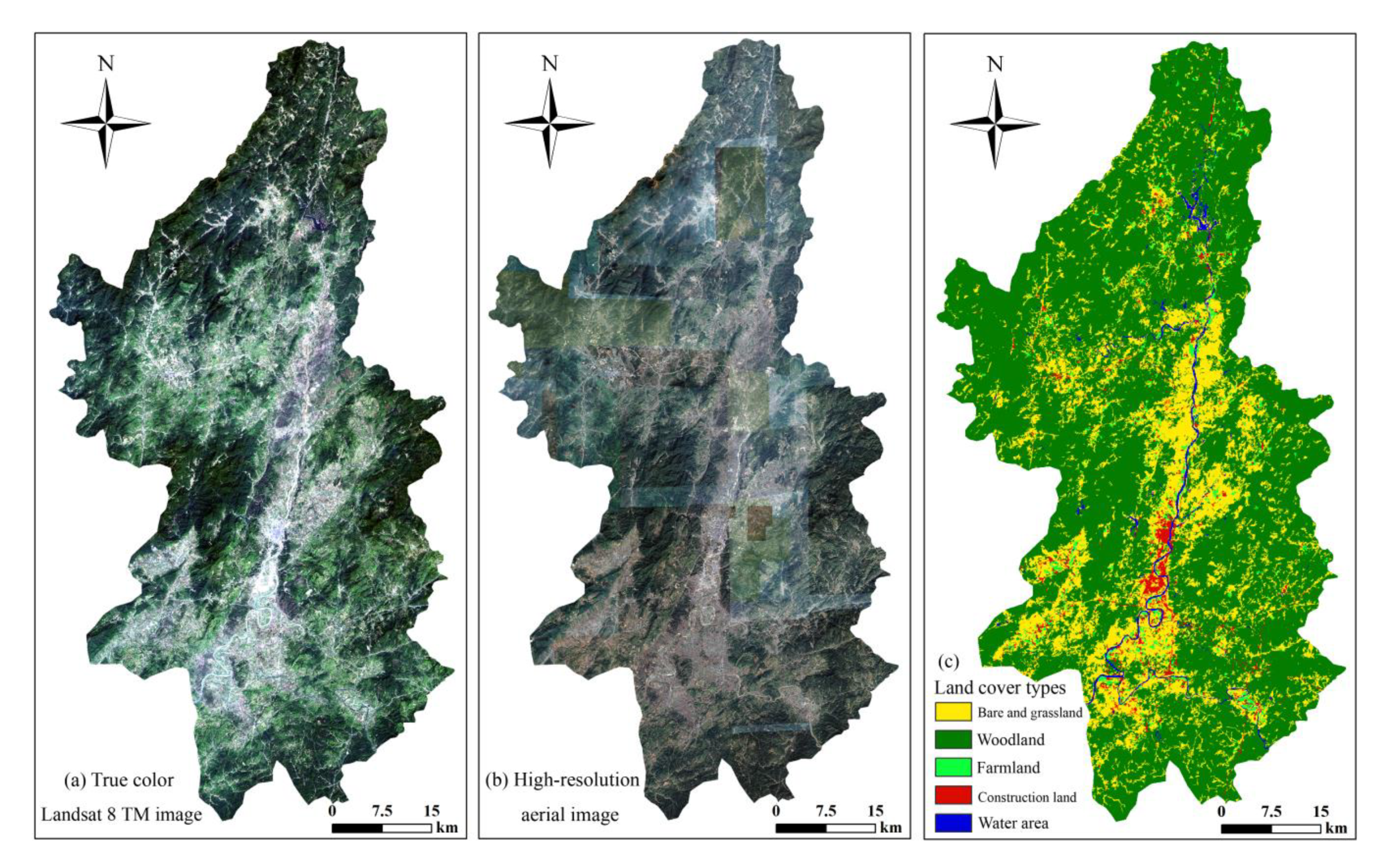
2.1.2. Acquisition and Description of Landslide Conditioning Factors

Landslides are caused by the effect of basic conditioning factors and inducing factors. The basic conditioning factors refer to the inherent characteristics of slopes, which include terrain, hydrological, land cover, and geography factors [33,40]. The inducing factors are the external conditions that induce landslides, such as earthquakes and heavy rainfall [44,45,46]. In general, the LSP reveals the instability probability of a slope when only considering the basic conditioning factors.

Generally, most of these basic conditioning factors are acquired from RS images and described in GIS software. The RS is mainly used to obtain conditioning factors. For example, the terrain and hydrological factors are extracted from Digital Elevation Model (DEM) through spatial analysis of ARCGIS software, land cover factors are extracted from high-resolution RS images. GIS is adopted as the basic platform of LSP to capture, analyze, store, and map spatial huge data of landslides [47]. In this study, grid units with resolution of 30 m × 30 m are selected as the basic mapping unit in ARCGIS. In addition, for predicting the landslide susceptibility indexes (LSIs) of Ningdu County, 12 conditioning factors are extracted as Figure 1 and Figure 2. Next, the nonlinear correlations between these landslides and conditioning factors are calculated by FR method in ARCGIS using spatial analysis functions.

Acquisition of Terrain Factors

The terrain factors of elevation, slope, slope aspect, profile curvature, plane curvature, relief amplitude are extracted through topographic spatial analysis of DEM in ARCGIS. Elevation is defined as the distance from a grid unit to the earth ellipsoid in the normal direction. Slope expresses the ratio of vertical height to the corresponding horizontal distance in a certain slope surface. The slope aspect, defined as the projection direction of the slope surface normal onto the horizontal plane, can be classified as flat, north, northeast, east, southeast, south, southwest, west, and northwest.

Meanwhile, the plane and profile curvatures respectively describe the vary features of concave and convex terrains from horizontal and vertical directions. Based on the definitions, the plane curvature and profile curvature are respectively calculated as the slope of the aspect and the slope of the slope in ARCGIS [7]. In addition, relief amplitude reflects the difference between the maximum elevation and minimum elevation in a certain area of one point on the ground surface [16]. The terrain amplitude can be obtained through the statistical test and the maximum height difference method in ARCGIS software for describing the regional macroscopic terrain characteristics. A greater relief amplitude means a higher terrain complexity.

Analysis of Hydrological Factors

The hydrological factors of Terrain Wetness Index (TWI) and drainage density are extracted through hydrological analysis method from DEM data. TWI reflects the important effect from the topography and soil moisture content on landslide occurrence, which is widely used in studies of hydrology, soil and geomorphology (Figure 3d). In addition, TWI can be expressed as $TWI=\ln \left(A_s/\tan \beta \right)$, where $A_s$ means the up-stream catchment area and $\beta$ presents the slope angle of a certain grid cell.

Drainage density reflects the ratio of total length of river network to per unit area. The drainage density shows the balance characteristics between climate, geomorphology, and hydrology (Figure 3e). Higher drainage density means that the basin is sensitive to rainfall, while lower drainage density means that the basin is insensitive to rainfall.

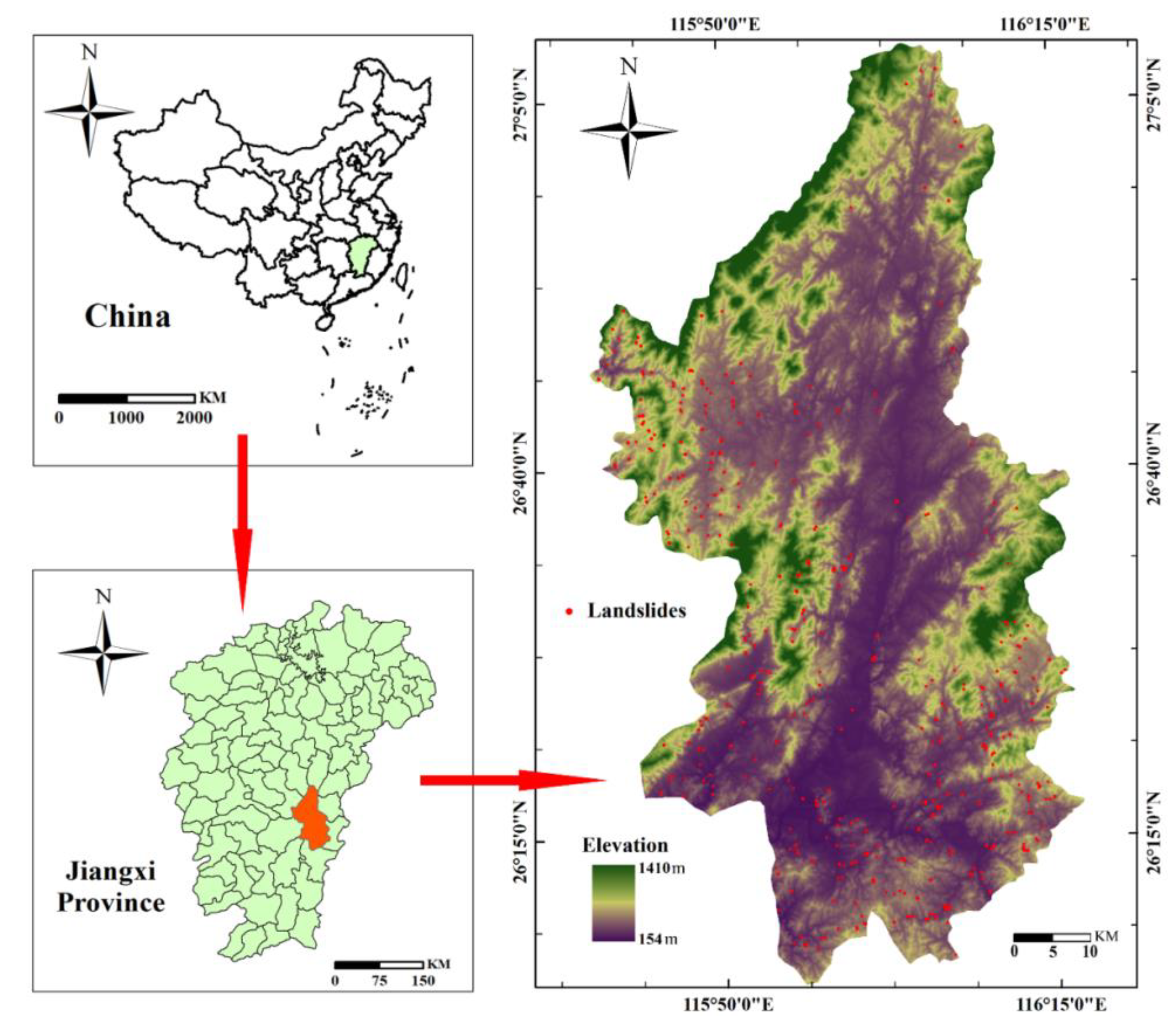
Land Cover and Geography Factors

The normalized difference built-up index (NDBI), normalized difference vegetation index (NDVI) are extracted from two Landsat TM 8 images (one on 15 October 2013, path/row 121/41 and one on 5 October 2013, path/row 121/42) (Figure 2a). The land cover types map of Ningdu County is produced through object-oriented image classification method. In additional, the geology factor of lithology is managed in ARCGIS, the physical and mechanical properties of rock mass usually change dramatically with lithological units.

The aerial image with raster resolution of 1.07 m, obtained from Google Earth 7.1.8.3036 (32-bit) on 12 January 2018, is used to map the land cover types distribution of Ningdu County (Figure 2b). In general, the land cover types of Ningdu County are classified as construction land, water, woodland, bare and grassland, and farmland. Then the object-oriented method is applied to map these land cover types of Ningdu County.

For the application of object-oriented method, the image objects are firstly segmented using multi-resolution segmentation method embedded within the eCognition Developer 8.7 software package. The scale, shape, and compactness parameters of multi-resolution segmentation method are respectively set to 30, 0.2, and 0.8 using “trial and error” method [48]. Secondly, some optimal features of image objects such as spectral attributes, layer values, geometry, position, and texture attributes are used as the input variables of 1-NN method (within the eCognition Developer 8.7) to classify these image objects. Meanwhile, thousands of training samples of each land cover type are determined through field survey and image interpretation. Finally, a land cover type classification map is produced as shown in Figure 2c.

It is necessary to assess the classification accuracy of this land cover map. Thousands of classified image objects are randomly chosen as reference samples to assess the classification accuracy. Then a multivariate statistical method namely Kappa Index of Agreement (KIA) is used as an accuracy evaluation index [49] (

Table 1. Assessment accuracy of land cover types map of Ningdu County using object-oriented method.

Accuracy	Woodland	Construction	Water	Bare and Grassland	Farmland
Producer’s	0.896	0.874	0.923	0.834	0.825
User’s	0.828	0.865	0.872	0.783	0.794
Total	Overall accuracy  0.857			KIA   0.825

). The classification accuracy of this aerial image is relatively low, especially due to the 2.07 m raster resolution and lack of NDVI feature (No near-infrared band in this aerial image). In additional, the image quality, segmentation method, and objects classification method also affect the classification accuracy of this image.

2.1.3. FR Analysis of Conditioning Factors

FR method is applied to determine the effects of conditioning factors on landslide occurrence [50]. As shown in

Table 2. Frequency ratios (FRs) of conditioning factors (aspect, plane curvature, profile curvature, NDVI are not presented).

Factor	Class	Landslide Not Occurred		Landslide Occurred		Frequency Ratio
		Count	Ratio (%)	Count	Ratio (%)
Elevation	154~243	1,106,278	0.244	1038	0.280	1.145
	243~322	1,304,742	0.288	1291	0.348	1.207
	322~410	827,136	0.183	758	0.204	1.118
	410~509	537,255	0.119	378	0.102	0.859
	509~617	369,291	0.082	175	0.047	0.578
	617~750	239,354	0.053	68	0.018	0.347
	750~937	110,355	0.024	3	0.001	0.033
	937~1410	33,871	0.007	0	0.000	0.000
Slope	0~3	975,826	0.215	150	0.040	0.188
	3~7	1,036,313	0.229	945	0.255	1.113
	7~11	848,288	0.187	1210	0.326	1.741
	11~15	652,842	0.144	742	0.200	1.387
	15~19	477,241	0.105	399	0.108	1.020
	19~24	315,595	0.070	179	0.048	0.692
	24~30	167,758	0.037	72	0.019	0.524
	30~53	54,419	0.012	14	0.004	0.314
Relief amplitude	0~39.673	1,005,640	0.222	610	0.164	0.740
	39.673~73.395	999,298	0.221	1430	0.385	1.746
	73.395~107.116	871,091	0.192	830	0.224	1.163
	107.116~142.822	675,230	0.149	402	0.108	0.726
	142.822~182.495	482,321	0.107	315	0.085	0.797
	182.495~230.102	301,925	0.067	110	0.030	0.445
	230.102~299.529	155,304	0.034	14	0.004	0.110
	299.529~505.827	37,473	0.008	0	0.000	0.000
Lithology	B3	222,246	0.049	35	0.009	0.192
	Y2	2,128,746	0.470	1460	0.393	0.837
	B1	1,310,225	0.289	1698	0.458	1.581
	B2	42,542	0.009	4	0.001	0.115
	S2	699,839	0.155	360	0.097	0.628
	S5	60,439	0.013	72	0.019	1.454
	S4	35,181	0.008	50	0.013	1.734
	T1	26,595	0.006	32	0.009	1.468
	W	2,469	0.001	0	0.000	0.000
TWI	3.898~6.583	1,262,093	0.279	1176	0.317	1.137
	6.583~8.261	1,719,261	0.380	1637	0.441	1.162
	8.261~10.275	975,276	0.215	668	0.180	0.836
	10.275~12.792	370,858	0.082	156	0.042	0.513
	12.792~16.483	156,837	0.035	53	0.014	0.412
	16.483~26.384	39,565	0.009	21	0.006	0.648
	26.384~39.137	4,123	0.001	0	0.000	0.000
	39.137~46.688	269	0.000	0	0.000	0.000
Drainage density	0~0.590	599,996	0.132	545	0.147	1.108
	0.590~1.067	861,429	0.190	525	0.141	0.744
	1.067~1.486	936,702	0.207	845	0.228	1.101
	1.486~1.886	778,759	0.172	672	0.181	1.053
	1.886~2.324	666,657	0.147	446	0.120	0.816
	2.324~2.876	398,554	0.088	258	0.070	0.790
	2.876~3.562	211,146	0.047	288	0.078	1.664
	3.562~4.857	75,039	0.017	132	0.036	2.146
NDBI	0~0.129	769,254	0.170	304	0.082	0.482
	0.129~0.172	1,255,933	0.277	813	0.219	0.790
	0.172~0.220	971,886	0.215	938	0.253	1.178
	0.220~0.270	593,484	0.131	720	0.194	1.480
	0.270~0.326	420,316	0.093	484	0.130	1.405
	0.326~0.384	289,927	0.064	271	0.073	1.141
	0.384~0.455	164,850	0.036	124	0.033	0.918
	0.455~1	62,632	0.014	57	0.015	1.111
Land cover	Bare and grassland	1,301,005	0.287	1,103	0.297	1.035
	Woodland	2,587,930	0.572	2,453	0.661	1.157
	Farmland	380,006	0.084	61	0.016	0.196
	Construction	102,625	0.023	94	0.025	1.118
	Water	56,716	0.0123	0	0.000	0.000

, for example, the FR values of elevation between 154 m and 410 m are greater than 1, suggesting landslides more probably occur in this elevations. The lithology map is produced through a geological map at a scale of 1:100,000. In this study, the lithology can be divided into 8 classes: hard clumpy intrusion rock (Y2); limestone and dolomite rock (T1); slate, metaclastics and phyllite (B1); schist (B2); clumpy chorismite (B3); sandstone, glutenite, and mudstone (S2); coal sandstone, shale, and mudstone (S4); and sandstone, glutenite, and shale (S5) (Figure 3f).

2.1.4. Correlation Analysis of Conditioning Factors

Before the LSP analysis, it is necessary to analyze the correlation between these 11 conditioning factors. The calculation results of correlation in the SPSS 22 software show that, correlation coefficient values between NDVI and NDBI, land cover are respectively 0.597 and 0.341, illustrating that NDVI has significant correlations with NDBI and land cover factors. Meanwhile, the correlation coefficient value between NDBI and Land cover is 0.257, suggesting that the correlation between NDVI and Land cover is stronger than that between NDBI and Land cover. In addition, the other correlation coefficient values are all smaller than a value of 0.26, which suggests that there are weak correlations between the other conditioning factors except NDVI. Hence, it is determined to implement the LSP using the above 10 conditioning factors except NDVI.

2.2. Methods

This research has several steps. (1) The landslides and related conditioning factors are acquired using “3S” (GPS, RS, and GIS) technology; (2) These conditioning factors are managed and saved using GIS software, and their FRs are calculated; (3) SML model is first trained using the known training sample dataset (such as labeled data and prior probability) to establish the sample learning model, and then this model is applied to predict and classify the remaining unknown data samples in GIS; (4) USML, a teacher-free learning method, refers to the automatic recognition of data samples by analyzing the internal similarities and external differences in the data sample itself without a known training sample dataset; (5) the corresponding LSMs of these SML and USML models are produced in ARCGIS software; Finally, the receiver operation curve (ROC) and FR accuracy are used to compare the prediction results for choosing the best prediction model and obtaining the most accurate LSP results of Ningdu County.

2.2.1. Acquisitions of Land Cover Factors from RS Images

Two important remote sensing indexes, NDVI and NDBI [51], are extracted from the Landsat TM images. NDVI is generally adopted for the detection of vegetation growth and coverage conditions as shown in Equation (1). NDBI is used to calculate the building distribution information on the surface of the landslide as shown in Equation (2).

$$NDVI=\frac{P\left(NIR\right)-P\left(Red\right)}{P\left(NIR\right)+P\left(Red\right)}$$

(1)

$$NDBI=\frac{P\left(MIR\right)-P\left(NIR\right)}{P\left(MIR\right)+P\left(NIR\right)}$$

(2)

where $P\left(Red\right)$ $P\left(NIR\right)$ and $P\left(NIR\right)$ are the measurements of spectral reflectance obtained in the visible red band, near infrared band, and middle infrared band of Landsat 8 TM image, respectively. Land cover types can be mapped by the RS image classification method [52]. The object-oriented method is used to map land cover types from high-resolution images because it can extract properties information from image objects (including spectral, geometrical, positional, and other features). The object-oriented method includes three steps: (1) The land cover types of the RS images are identified through field survey and visual interpretations on high-resolution image; (2) The image objects are extracted from the RS images using multi-resolution segmentation method and their corresponding classification features are selected; (3) The obtained image objects are classified into several land cover types using the simple nearest neighbour (1-NN) method [53], which is a highly efficient and accurate image classification model and is not built based on a Gaussian distribution.

2.2.2. Drainage Density Extraction by Hydrological Analysis Tool

The river network of a study area can be extracted by the hydrological analysis tool of ARCGIS software [54]. The DEM data with resolution of 30 m is selected as the basis data. Firstly, the depressions of DEM are filled by the Fill tool. Then the water flow direction of DEM is calculated by the Flow Direction tool. Based on this data, the flow accumulation can be obtained by the Flow Accumulation tool. In the next step, the river network is generated through selecting the flow accumulation of each grid unit above a certain threshold. The flow accumulation threshold of this study is selected to 5000. Finally, the drainage density can be calculated by grid calculator as shown in Equation (3), where $D_S$ is drainage density; $\sum L$ is length of river networks in a unit area $A$.

$$D_S={\displaystyle \sum L/A}$$

(3)

2.2.3. FR Method

FR method is introduced to discuss the effects of conditioning factors on landslides susceptibility. All the conditioning factors are divided into 8~9 classes using the natural break point method (the lithology is divided by strata configuration and the land cover is divided to 5 classes). Finally, the FR values is calculated using Equation (4) and is shown in Table 2. An FR value greater than 1, indicates a higher correlation between landslide and conditioning factors; whereas an FR value that is lower than 1, suggests a lower effect on landslide.

$$FR=\frac{A/A\prime }{B/B\prime }$$

(4)

where $A$ donates the pixels number of the landslide in each class of conditioning factor,$A\prime$ donates the pixels number of the total landslides in Ningdu County, $B$ suggests the pixels number in the class of the factor; $B\prime$ suggests the number of total pixels in the whole study area.

2.2.4. Supervised Machine Learning

SVM Model

SVM is a type of very popular SML methods for dealing with the problems of classification and regression [21]. Suppose a series of training input $x_i (i=1,2,\dots ,n)$. The $y\left(y=\pm 1\right)$ corresponds to output of binary-classification problem. This method is aimed to search an n-dimensional hyper-plane which can differentiate the two classes by the gap with maximal value as:

$$\frac{1}{2}{\Vert w\Vert }^2$$

(5)

$$y_i\left(\omega \cdot x_i\right)+b\ge 1$$

(6)

where ${\Vert w\Vert }^2$ is the norm of the normal of the hyper-plane, b is regarded as a constant value. The Lagrangian forma is used to define the cost function as:

$$L={\Vert w\Vert }^2/2-{\displaystyle \sum _{i=1}^N{\lambda }_i\left(\left(y_i\left(\omega \cdot x_i\right)+b\right)-1\right)}$$

(7)

$$y_i\left(\omega \cdot x_i\right)+b\ge 1$$

(8)

where ${\lambda }_i$ is the Lagrange multiplier. The slack variable ${\xi }_i$ is used as the non-separable case which is modified as:

$$y_i\left(\left(\omega \cdot x_i\right)+b\right)\ge 1-{\xi }_i$$

(9)

Then Equation (7) can be expressed as Equation (10), where $v\left(0,1\right]$ reflects the problem of misclassification. Meanwhile, the radial basis function is selected as the kernel function of SVM.

$$L=\frac{1}{2}{\Vert w\Vert }^2-\frac{1}{vn}{\displaystyle \sum _{i=1}^n{\xi }_i}$$

(10)

CHAID Model

CHAID is also one of the main supervised learning decision trees for regression and classification problems [55]. CHAID tree is built through classifying subsets of the variables into several child nodes. The dependent variables and conditioning factors are expressed to be nominal or continuous data. The CHAID establishes a framework with non-binary tree which contains several branches comparing to other decision trees. The classification iteration of CHAID will stop if any meaningful chi-square value between conditioning factors and related dependent variable cannot be found.

2.2.5. Unsupervised Machine Learning

K-Means Model

K-means clustering is regarded as an USML algorithm because it is an efficient unsupervised classification implementation. K-means clustering is mainly aimed to automatically partition a certain data set into K classes through comparing their Euclidean distance. The main iterative process of K-means clustering is as follows:

(1) Let $S=\left\{x_1,x_2,\cdots x_n\right\}$ and set the number of clusters K and the initial central point of each cluster, where $x_m\in R^n$ and $m$ represents the number of points.

(2) For each point $x_i$ in the $S$ dataset, its Euclidean distances to the K central points are calculated, and then each point is classified into the corresponding cluster with the smallest distance to the central point of the cluster. The Euclidean distances between all points are expressed as:

$$D={\left({\displaystyle \sum _{i=1}^n{\left(x_i-m_i\right)}^2}\right)}^{1/2}$$

(11)

(3) All the data points are re-clustered, then the centroids of these data points are updated repeatedly until the centroids of data points do not change.

Kohonen Model

The Kohonen model is a feed-forward ANN based on an unsupervised learning algorithm [56]. The Kohonen model is generally consisted by one input and one output layer (also called a competitive layer), and these two layers are connected by the weights. The number of input variables is regarded as the neurons number of input layer. Neurons in the output layer are represented on a two-dimensional lattice. The aim of the Kohonen model is to deal with a nonlinear mapping process of the high-dimensional input vectors into a low-dimensional map (two-dimensional grid).

3. Results

The LSP results in Ningdu County are predicted using the SML (SVM and CHAID models) and USML (K-means and Kohonen models) models for comparisons.

3.1. Results of the SML Models

3.1.1. Preparation Training and Validation Dataset

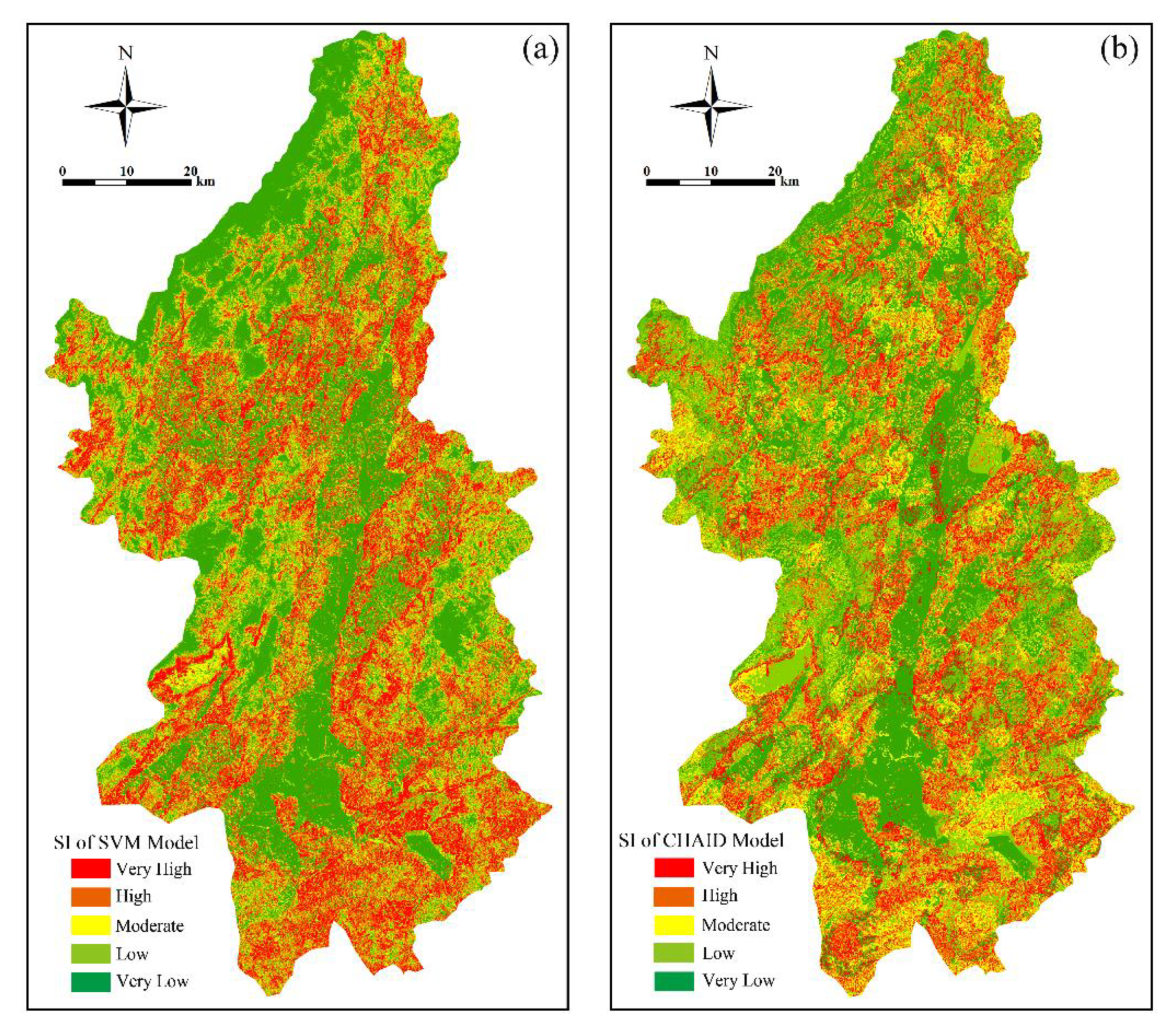
It is important and indispensable for SML models to obtain the training and testing dataset. The training dataset is generally applied for building these models, and the testing dataset is applied for validating these models and to confirm their accuracy. The dataset not only contains the landslide grid units but also contains the non-landslide grid units with the same number of landslide grid units. In this study, there are a total of 3711 landslide grid units that are assigned to 1. The same number of non-landslide grid units are assigned to 0, are sampled randomly from the landslide-free area. Therefore, the dataset of landslide and non-landslide grid units is randomly spilt into a training dataset and a testing dataset with a ratio of 70:30, to map the landslide susceptibility using SVM and CHAID models.

3.1.2. SVM Model

The SVM model is trained based on the ten-fold cross-testing method. In the training process, the optimum values of γ and regression precision are respectively determined to be 0.1 and 0.1. Then, the trained SVM model is applied for all the grid samples of Ningdu County. Moreover, the LSP indexes are calculated as values ranging from 0 to 0.982. Next, all LSIs are imported into ArcGIS 10.2 for producing corresponding LSM. Last, the obtained LSM is reclassified into five classes based on the natural break method to better observe the results (Figure 4a). The natural break method is used for all the present models. Very high susceptibility (0.770~0.982), high susceptibility (0.581~0.770), moderate susceptibility (0.370~0.581), low susceptibility (0.166~0.370), and very low susceptibility (0~0.166) classes cover 20.20%, 17.55%, 14.79%, 15.32%, and 32.14% in Ningdu County, respectively.

3.1.3. CHAID Model

To achieve the desirable LSP results in the CHAID model, it is important to set up suitable model criteria. The maximum value of tree depth is set as 10. The limit of the statistical significance, which controls the merger and creation of new branches, is set as 0.05. The Pearson statistical test is used for the chi-square statistic because it is suitable for the large dataset. The results of the CHAID model are shown with the tree structure consisting of many branches representing the related classification of each landslide related conditioning factor. In addition, the tree depth value is 5, while the node number is 92. Some other model parameters are also revealed. Finally, the LSP indexes ranging from 0 to 1 are determined into five classes and then are constructed as a LSM ArcGIS 10.2 (Figure 4b and

Table 3. The frequency ratio among the landslide susceptibility classes for different models.

Model	Class	Landslide Pixels	Percentage of Landslide Pixels (%)	Pixels in Domain	Percentage of Pixels in Domain (%)	Frequency Ratio
SVM	Very High	2202	0.593	914,815	0.202	2.937
	High	770	0.207	794,803	0.176	1.182
	Moderate	360	0.097	669,532	0.148	0.656
	Low	216	0.058	693,662	0.153	0.380
	Very Low	163	0.044	1,455,470	0.321	0.137
CHAID	Very High	1527	0.411	746,461	0.165	2.496
	High	1139	0.307	748,410	0.165	1.857
	Moderate	693	0.187	775,501	0.171	1.090
	Low	291	0.078	1,229,765	0.272	0.289
	Very Low	121	0.033	1,333,349	0.294	0.111
K-means	Very High	1384	0.373	787,386	0.174	2.145
	High	930	0.251	870,420	0.192	1.304
	Moderate	1079	0.291	1,321,009	0.292	0.997
	Low	185	0.050	753,772	0.166	0.299
	Very Low	133	0.036	795,695	0.176	0.204
Kohonen	Very High	1846	0.497	1,059,768	0.234	2.126
	High	982	0.265	953,143	0.210	1.257
	Moderate	447	0.120	830,506	0.183	0.657
	Low	305	0.082	1,016,018	0.224	0.366
	Very Low	131	0.035	668,849	0.148	0.239

).

3.2. Results of USML Models

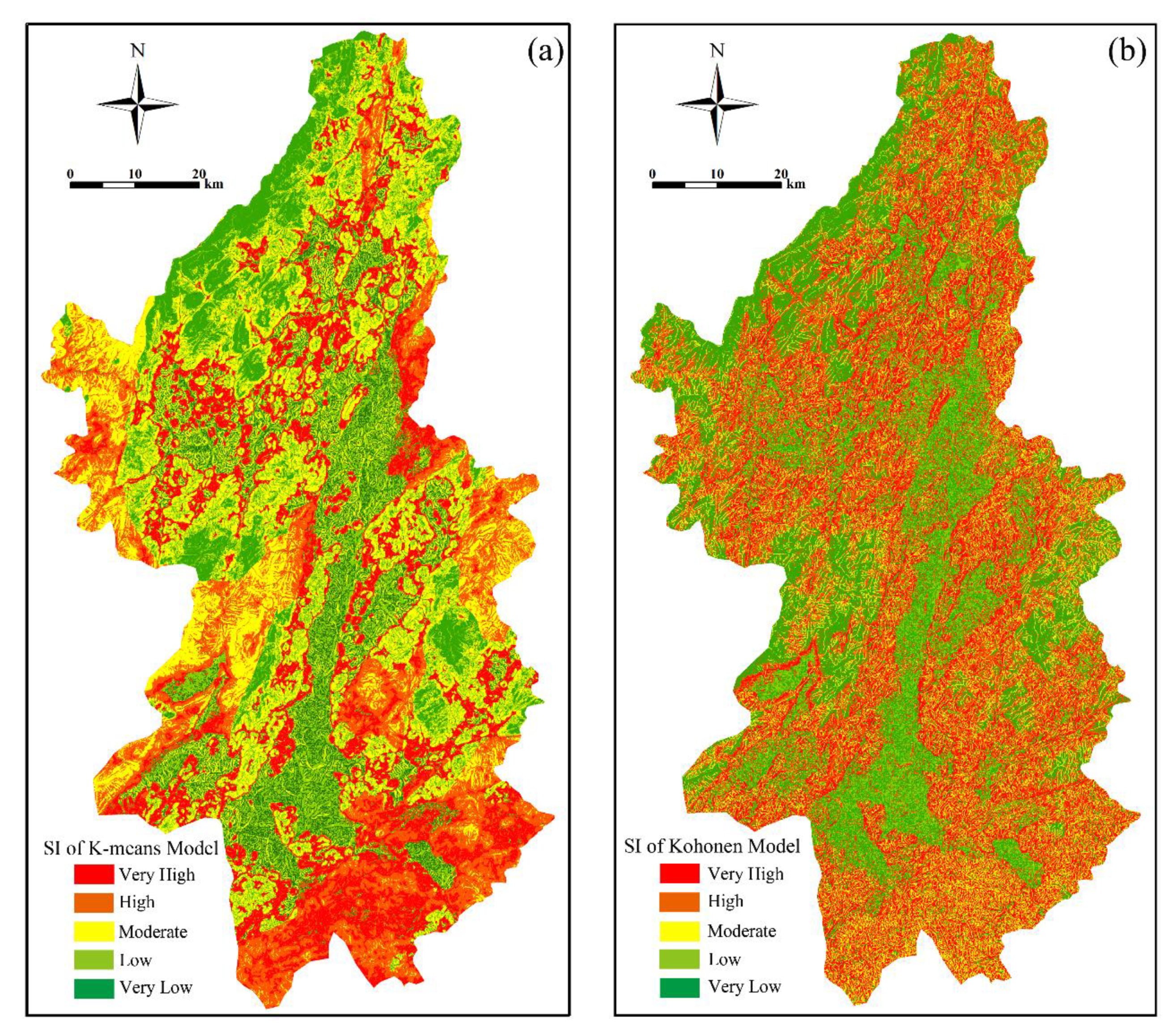
3.2.1. K-Means for LSP

The selected normalized conditioning factors are imported as the training dataset of K-means method. The clusters number is set to 5, the clustering central point is determined randomly, and the iteration number is set to 50. Then, each training data point is classified into the corresponding cluster with the smallest distance to the final clustering central point through 50 iterative calculations. The LSM is produced on the basis of the five clustering classes corresponding to very high, high, moderate, low, and very low (Figure 5a and Table 3).

3.2.2. Kohonen Model

For training Kohonen model, the input nodes number is set to 11 because 11 conditioning factors are standardized as the input vector. The maximum learning rate (rate1max) and the minimum learning rate (rate1min) are respectively 0.1 and 0.01. In addition, the maximum neighborhood radius (r1max) is set to 1.5, and the minimum neighborhood radius (r1min) is set to 0.4. The maximum iterations number is set to 1000, and the Kohonen model will stops until the iterations reach. The LSM produced by the Kohonen model and its landslide susceptibility classes are shown in Figure 5b and Table 3.

3.3. Models Testing and Comparison

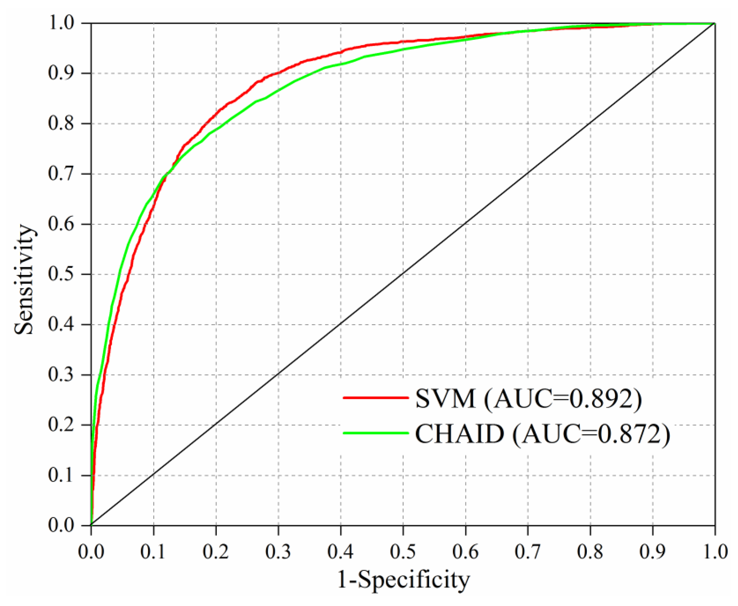
The model validation is an important and necessary step to examine the predictive accuracy and to compare the performance of different LSP models [57,58,59]. The curve of receiver operating characteristics (ROC) is introduced for evaluating the LSP performance of the SML models (SVM and CHAID model), while the frequency ratio (FR) accuracy is used for evaluating the LSP performance of all models.

3.3.1. ROC Curve

ROC analysis is commonly used for evaluating the LSP accuracy of different models, which indicates the correlation between sensitivity and specificity through the plotting method [50]. The area under ROC (AUC) is defined to assess the LSP accuracy of these models, containing values between 0.5 and 1.0. Larger AUC value means greater accuracy of model. Figure 6 shows that the AUC values of the SVM and CHAID models are respectively 0.892 and 0.872, suggesting both models have excellent and satisfied LSP performance, and further suggesting that the SVM has higher LSP accuracy than the CHAID model.

3.3.2. Frequency Ratio Accuracy Validation

The ROC method cannot be used for evaluating the USML. On the contrary, the FR accuracy, defined as the ratio of the sum of frequency ratios of high and very high LSLs to the total frequency ratios, can be used to evaluate both SML and USML models [60]. The FR accuracies of the SML and USML models are shown in Table 3, showing that FR values gradually decrease from the very high to the very low susceptibility classes.

For very high susceptibility class, the SVM has the highest FR value (2.937), followed by the CHAID (2.496), Kohonen (2.145), and K-means models (2.126). In addition, the FR accuracies of SVM, CHAID, K-Means, and Kohonen are respectively 0.778, 0.745, 0.697, 0.728. Therefore, the validation results confirm that SVM has the highest prediction performance, followed by CHAID, Kohonen and K-means method, further confirm that SML has higher LSP accuracy than that of USML.

4. Discussion

4.1. Comparison of Model Accuracy

This study deals with the comparisons of LSP results of the SML and USML models, showing that SML has higher LSP performance than USML. In addition, it can be seen from Figure 4 and Figure 5 that a large number of very high and high susceptibility classes locate in the south-east and north-west sections of Ningdu County and are mainly distributed in the zones near roads and rivers, which are consistent with the landslide distribution features.

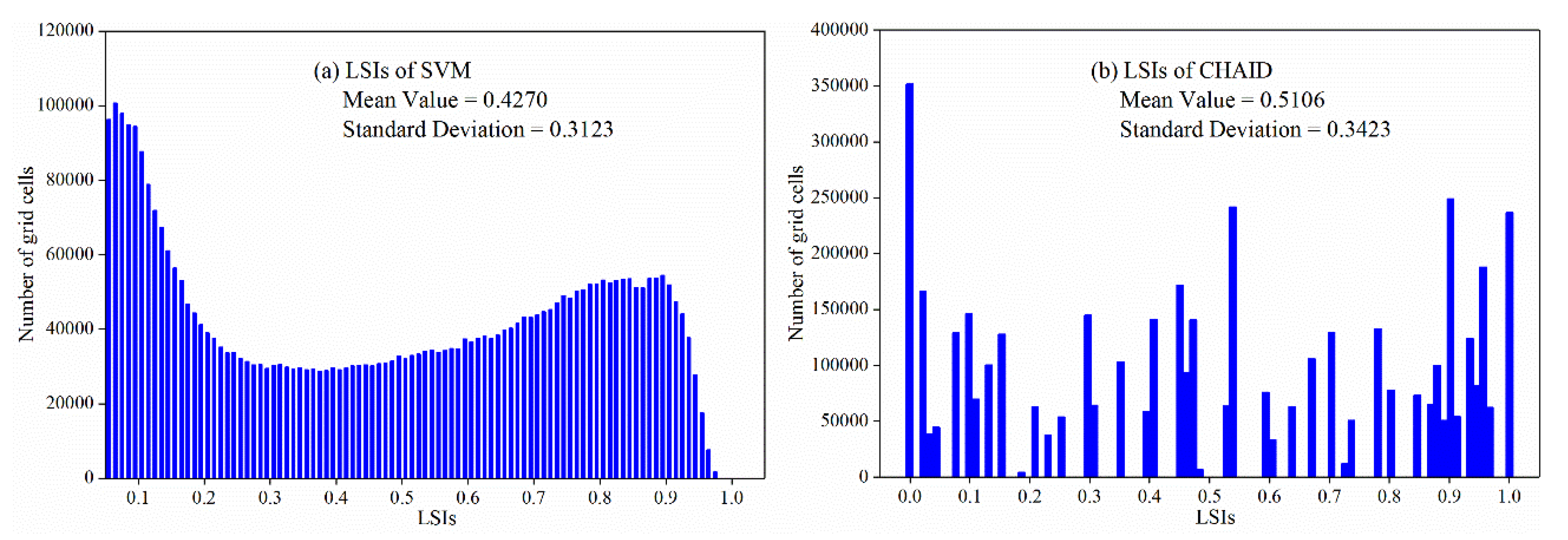
4.2. Distribution Features of LSIs

The SML models (SVM and CHAID models) can calculate the LSIs of the study area, while the USML models (K-means and Kohonen models) can only obtain the landslide susceptibility classes. The distribution features of LSIs with their corresponding mean values and standard deviations calculated by the SML models are shown in Figure 7. It can be seen from Figure 7 that the LSIs calculated by the SVM model mainly belong to low and/or very low landslide susceptibility classes with low degree of dispersion, while those calculated by CHAID model mainly belong to low and moderate landslide susceptibility classes with high degree of dispersion. Figure 7 also shows that the LSIs calculated by SVM model have higher continuity than that of CHAID model. In addition, the mean values and standard deviations suggest that SVM model has better LSP performance than the CHAID model. This is because the mean value of LSIs of SVM model (0.4270) is lower than that of CHAID model (0.5106), although the standard deviations of the two models are close.

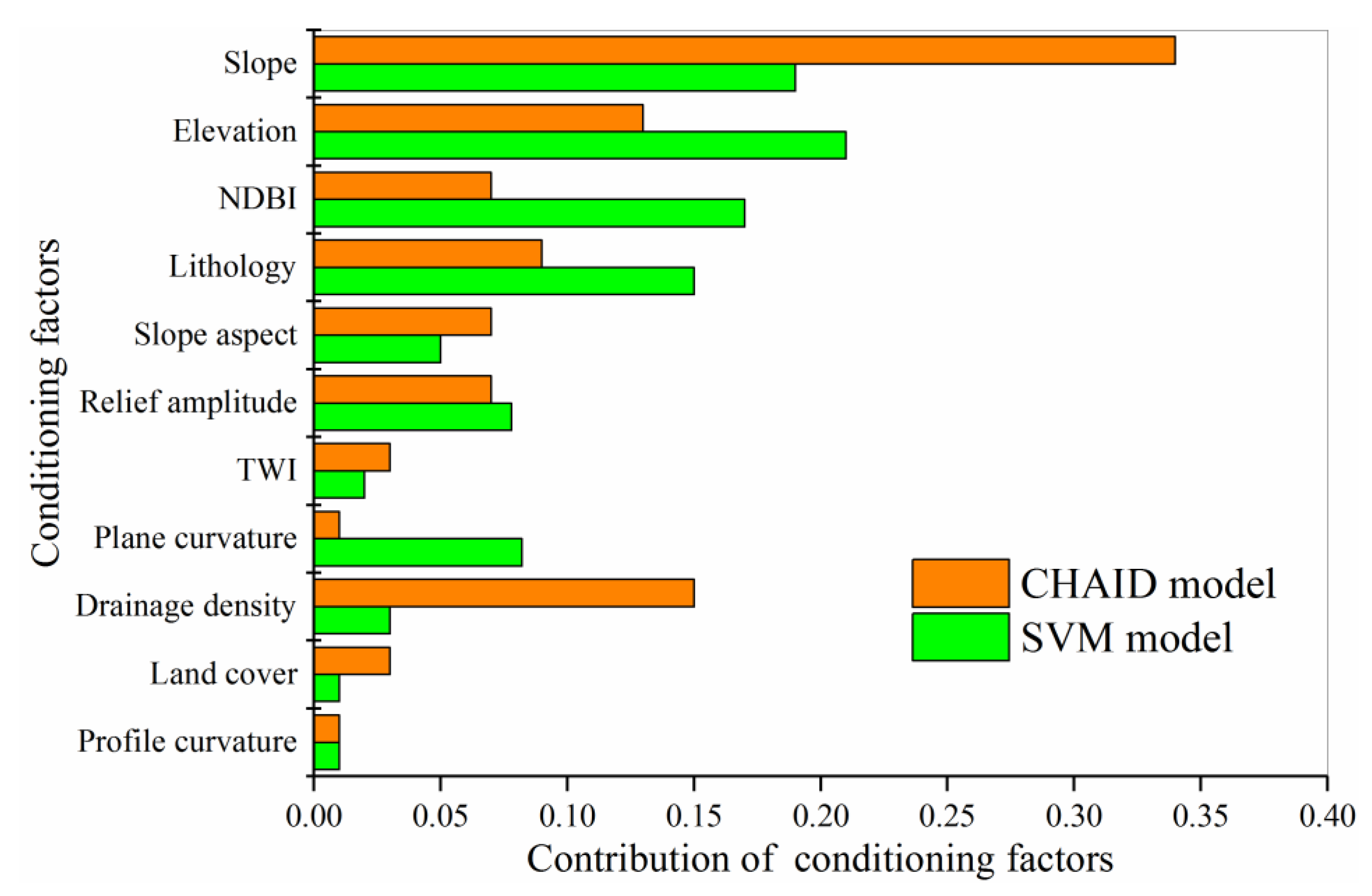
4.3. Relative Importance of Conditioning Factors for SML Models

The selection of landslide conditioning factors plays an important role in the LSP, however, it is still a topic to debate [61]. Therefore, in this study, the relative importance of conditioning factors is also analyzed by both SML models (Figure 8). The ability of identifying the relative importance of conditioning factors is another advantage of SML models comparing to USML models.

Figure 8 shows that all the eleven conditioning factors have positive contributions to LSP modeling in a certain extent for different models. In case of SVM model, the elevation, slope, NDBI, and Lithology factors have the highest contributions of 21.00%, 19.00%, 17.00%, and 15.00%, respectively. For the CHAID model, the slope, drainage density, and elevation factors have the highest contributions of 34.00%, 15.00%, 13.00%, and 15.00%, respectively. The other conditioning factors have smaller contributions to the SVM and CHAID models. The results indicate that the contributions of different conditioning factors to the LSP are similar with each other in the different LSP models for a certain study area.

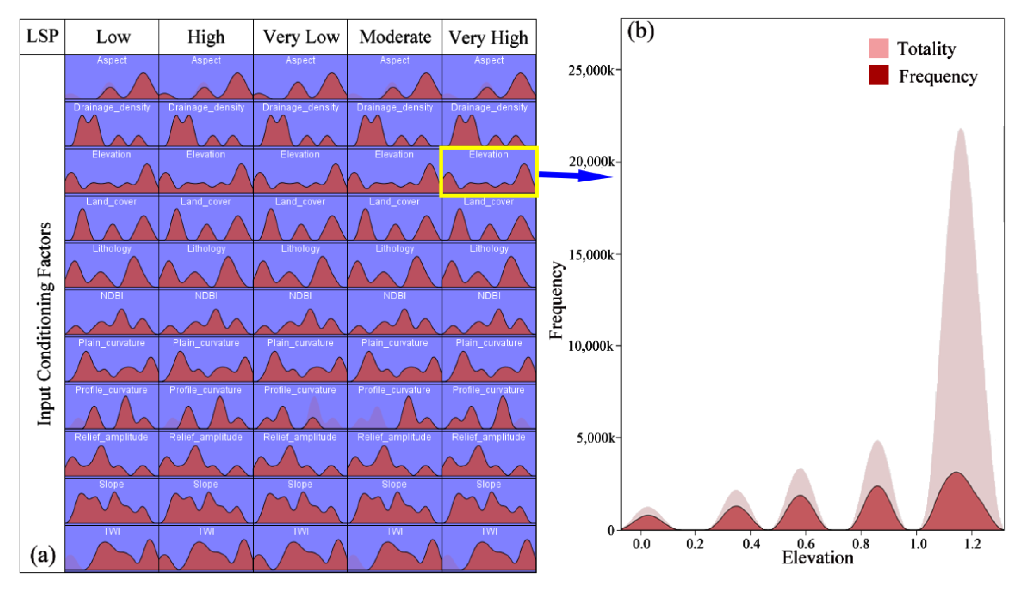
4.4. Conditioning Factors Distribution Using USML Models

Comparing to the results of SML (SVM and CHAID) models, the clustering information of conditioning factors can be well revealed by the USML (K-means and Kohonen) models. The frequency distribution of conditioning factors for each LSP class of Kohonen model is shown in Figure 9a. For example, Figure 9b shows the frequency of elevation for very high class of LSP. Meanwhile, for the K-means model, the clustering centers of conditioning factors for each LSP class can also be shown visually. These results show that the USML has batter data interpretation than that of SML, because the conditioning factors data can be clustered into five types of group according to the consistency of data characteristics.

4.5. Sensitivity Analysis on Resolution of Grid Units

It is very important to select an appropriate grid resolution for LSP. Too low resolution cannot guarantee the rationality of the obtained LSP, while too high resolution will greatly increase the model computation complexity [62]. Although some studies focusing on the issue of LSP considering the different spatial resolutions of grid units, show that the LSP performance decreases when the resolution of grid units rises from 10 m to 100 m [63], a lot of literature shows that a 30 m grid resolution is suitable for LSP and can obtain satisfactory LSP results [7,11,21,30,35,37,50,59,64,65,66,67,68,69]. Meanwhile, the original grid resolutions of the DEM and remote sensing images used in this study are both 30 m, which can not only effectively represent the topographic characteristics, but also avoid excessive computation. Therefore, this study adapts the grid unit with 30 m resolution for LSP.

4.6. Analysis of Parameters of Model Itself

It is revealed in this study that different ML models exhibit different LSP performances based on the same input data, this is because that some parameters of model itself (including activation functions, model structures, learning rate, etc.) have considerably different effects on LSP results.

For the SVM modeling, it is well-known that the prediction performance of SVM model is influenced by the selection of kernel function and other corresponding parameters (width value of kernel function and regression precision). Hong et al. [70] suggested that the radial basis function kernel function can achieve the best LSP performance comparing to the polynomial, sigmoid, and linear kernel functions. In addition, N-fold cross-testing method is used to determine the corresponding parameters of SVM, because N-fold cross-testing method is an efficient and global parameters searching algorithm and it is appropriate for huge data modeling [16].

For the decision trees of Classification & Regression Tree (C&RT) model and CHAID model, the C&RT model is a binary tree (two branches in each node), while the CHAID model is built based on the non-binary tree framework and contains two or more branches growing from a single node [71]. Park, Lee, Lee, and Lee [26] have compared and analyzed the LSP performances under the conditions of different decision tree structures, and indicated that the CHAID model has the highest accuracy. Moreover, the CHAID model can be controlled by pre-setting the model’s criteria (e.g., growth limit and merging value) to avoid over-fitting problem.

For the K-means clustering and Kohonen models, the main model parameters are clustering number and iteration number. The clustering number can be determined by the number of LSM class. The iteration number is used to end the clustering process and is to meet the data convergence. In addition, the learning rate, the neighbor-hood radius in Kohonen model should be reasonably selected to ensure the accuracy and validity of the LSP result. In this study, although the Kohonen model has a better LSP performance than K-means model, the learning rate of K-means model (time is 260s) is greater than that of Kohonen model (time is 680s).

4.7. Comparison Analysis of SML and USML

There are some differences in the LSP modeling of SML and USML: (1) the core of SML is prediction and classification, which means that the data are classified by selecting classifiers and determining weights. The core of USML is cluster analysis, which divides datasets into classes with similar objects. Hence, USML algorithms can start working as long as they know how to calculate similarity. (2) SML is usually poor to reduce data dimensions. In contrast, USML achieves dimensionality reduction of data by using layer clustering or item clustering. Furthermore, the USML results exhibit as a group of clusters by clustering first and then qualitatively analyzing. (3) The classification reasons for SML are unexplainable because classification principles are artificially generated. USML is a useful interpretation of the clustering method; that is, the data can cluster into a group according to the consistency of data characteristics. (4) The scalability of SML is weak. By contrast, the scalability of USML is strong, and regardless of how high the weight of the additional one-dimensional data is, it will have a limited effect on the original result output.

The recorded landslides, as prior knowledge, play a core role for training and testing processes of the SML model, contributing to the high prediction accuracy. The lack of a strong target in the modeling process is an important reason for the low prediction accuracy of the USML model. This is because there are no prior training samples and supervised information to be used in the USML model, and if there are some marginalization test samples continuing to be accepted by the classifier, the accuracy of the classification may be affected. On the other hand, the difficult acquisition of training samples, the accuracy of training samples and the small number of training samples also have a negative effect on the prediction results. Hence, it is recommended to use a semi-supervised machine learning method for LSP, which can solve the problems of the weak generalization ability of SML and the imprecision of USML. In addition, the uncertainty and analysis errors of the prediction models also have a certain impact on the prediction results. This can be seen by comparing the results of the SVM and CHAID models; the ROC accuracy of the two models is similar (Figure 4), while the FR accuracy is quite different (Table 3) due to the differences in the internal algorithms of the two models, which leads to many very high class pixels being classified as moderate class in the CHAID model. Therefore, use of integrated learning to comprehensively evaluate the prediction results of each model is suggested.

5. Conclusions

In this study, 446 recorded landslides and landslide-related conditioning factors are acquired, stored and analyzed through RS and GIS technologies. Then, the LSMs of Ningdu County have been predicted using SML models (SVM and CHAID models) and USML models (K-means and Kohonen models) based on the 11 conditioning factors. In general, ML models have been successfully used to carry out LSP with the SVM having the greatest LSP accuracy, followed by CHAID, Kohonen, and K-means models. Furthermore, the SML models have better LSP performance than the UMSL models because the SML models trained with recorded landslide training samples have strong predictive power for unknown data, while the lack of a strong target in the USML model leads to limited prediction accuracy. However, difficult acquisition of training samples, the accuracy of training samples and a small number of training samples have negative effects on the prediction results of SML models.

In addition, the UMSL models have also been widely used in LSP due to some advantages, such as simple modeling, efficiency, dimensionality reduction and scalability, compared to the SML models. Hence, it is recommended to improve the prediction accuracy of SML and USML models in further research in order to reduce the uncertainty and analysis errors associated with ML models. As a final conclusion, the results from comparisons of SML and USML for producing LSMs may be meaningful for making correct decision about land use planning in areas prone to landslides.

References

1. Turner, D.; Lucieer, A.; de Jong, S. Time series analysis of landslide dynamics using an unmanned aerial vehicle (UAV). Remote Sens. 2015, 7, 1736–1757. [Google Scholar] [CrossRef] [Green Version]
2. Shao, X.; Ma, S.; Xu, C.; Zhang, P.; Wen, B.; Tian, Y.; Zhou, Q.; Cui, Y. Planet Image-Based Inventorying and Machine Learning-Based Susceptibility Mapping for the Landslides Triggered by the 2018 Mw6. 6 Tomakomai, Japan Earthquake. Remote Sens. 2019, 11, 978. [Google Scholar] [CrossRef] [Green Version]
3. Assilzadeh, H.; Levy, J.K.; Wang, X. Landslide catastrophes and disaster risk reduction: A GIS framework for landslide prevention and management. Remote Sens. 2010, 2, 2259–2273. [Google Scholar] [CrossRef] [Green Version]
4. Pradhan, B. Remote sensing and GIS-based landslide hazard analysis and cross-validation using multivariate logistic regression model on three test areas in Malaysia. Adv. Space Res. 2010, 45, 1244–1256. [Google Scholar] [CrossRef]
5. Guzzetti, F.; Carrara, A.; Cardinali, M.; Reichenbach, P. Landslide hazard evaluation: A review of current techniques and their application in a multi-scale study, Central Italy. Geomorphology 1999, 31, 181–216. [Google Scholar] [CrossRef]
6. Park, H.J.; Jang, J.Y.; Lee, J.H. Physically based susceptibility assessment of rainfall-induced shallow landslides using a fuzzy point estimate method. Remote Sens. 2017, 9, 487. [Google Scholar] [CrossRef] [Green Version]
7. Huang, F.; Yao, C.; Liu, W.; Li, Y.; Liu, X. Landslide susceptibility assessment in the Nantian area of China: A comparison of frequency ratio model and support vector machine. Geomat. Nat. Hazards Risk 2018, 9, 919–938. [Google Scholar] [CrossRef] [Green Version]
8. Althuwaynee, O.F.; Pradhan, B.; Park, H.J.; Lee, J.H. A novel ensemble bivariate statistical evidential belief function with knowledge-based analytical hierarchy process and multivariate statistical logistic regression for landslide susceptibility mapping. Catena 2014, 114, 21–36. [Google Scholar] [CrossRef]
9. Pourghasemi, H.R.; Beheshtirad, M.; Pradhan, B. A comparative assessment of prediction capabilities of modified analytical hierarchy process (M-AHP) and Mamdani fuzzy logic models using Netcad-GIS for forest fire susceptibility mapping. Geomat. Nat. Hazards Risk 2016, 7, 861–885. [Google Scholar] [CrossRef] [Green Version]
10. Sezer, E.A.; Nefeslioglu, H.A.; Osna, T. An expert-based landslide susceptibility mapping (LSM) module developed for Netcad Architect Software. Comput. Geosci. 2017, 98, 26–37. [Google Scholar] [CrossRef]
11. Dikshit, A.; Sarkar, R.; Pradhan, B.; Jena, R.; Drukpa, D.; Alamri, A.M. Temporal Probability Assessment and Its Use in Landslide Susceptibility Mapping for Eastern Bhutan. Water 2020, 12, 267. [Google Scholar] [CrossRef] [Green Version]
12. Weidner, L.; Oommen, T.; Escobar-Wolf, R.; Sajinkumar, K.; Samuel, R.A. Regional-scale back-analysis using TRIGRS: An approach to advance landslide hazard modeling and prediction in sparse data regions. Landslides 2018, 15, 2343–2356. [Google Scholar] [CrossRef]
13. Ciurleo, M.; Mandaglio, M.C.; Moraci, N. Landslide susceptibility assessment by TRIGRS in a frequently affected shallow instability area. Landslides 2019, 16, 175–188. [Google Scholar] [CrossRef]
14. Sinarta, I.N.; Rifa’i, A.; Faisal Fathani, T.; Wilopo, W. Slope stability assessment using trigger parameters and SINMAP methods on Tamblingan-Buyan ancient mountain area in Buleleng Regency, Bali. Geosciences 2017, 7, 110. [Google Scholar] [CrossRef] [Green Version]
15. Huang, F.; Huang, J.; Jiang, S.; Zhou, C. Landslide displacement prediction based on multivariate chaotic model and extreme learning machine. Eng. Geol. 2017, 218, 173–186. [Google Scholar] [CrossRef]
16. Huang, F.; Yin, K.; Huang, J.; Gui, L.; Wang, P. Landslide susceptibility mapping based on self-organizing-map network and extreme learning machine. Eng. Geol. 2017, 223, 11–22. [Google Scholar] [CrossRef]
17. Pandey, V.K.; Sharma, K.K.; Pourghasemi, H.R.; Bandooni, S.K. Sedimentological characteristics and application of machine learning techniques for landslide susceptibility modelling along the highway corridor Nahan to Rajgarh (Himachal Pradesh), India. Catena 2019, 182, 104150. [Google Scholar] [CrossRef]
18. Huang, F.; Wang, Y.; Dong, Z.; Wu, L.; Guo, Z.; Zhang, T. Regional landslide susceptibility mapping based on grey relational degree model. Earth Sci. 2019, 44, 664–676. [Google Scholar]
19. Huang, F.; Yin, K.; Zhang, G.; Gui, L.; Yang, B.; Liu, L. Landslide displacement prediction using discrete wavelet transform and extreme learning machine based on chaos theory. Environ. Earth Sci. 2016, 75, 1376. [Google Scholar] [CrossRef]
20. Mutlu, B.; Nefeslioglu, H.A.; Sezer, E.A.; Akcayol, M.A.; Gokceoglu, C. An Experimental Research on the Use of Recurrent Neural Networks in Landslide Susceptibility Mapping. ISPRS Int. J. Geo-Inf. 2019, 8, 578. [Google Scholar] [CrossRef] [Green Version]
21. Su, Q.; Zhang, J.; Zhao, S.; Wang, L.; Liu, J.; Guo, J. Comparative assessment of three nonlinear approaches for landslide susceptibility mapping in a coal mine area. ISPRS Int. J. Geo-Inf. 2017, 6, 228. [Google Scholar] [CrossRef] [Green Version]
22. Huang, F.; Yin, K.; He, T.; Zhou, C.; Zhang, J. Influencing factor analysis and displacement prediction in reservoir landslides—A case study of Three Gorges Reservoir (China). Tehnički Vjesnik 2016, 23, 617–626. [Google Scholar]
23. Huang, F.; Huang, J.; Jiang, S.H.; Zhou, C. Prediction of groundwater levels using evidence of chaos and support vector machine. J. Hydroinformatics 2017, 19, 586–606. [Google Scholar] [CrossRef] [Green Version]
24. Dou, J.; Yunus, A.P.; Tien Bui, D.; Merghadi, A.; Sahana, M.; Zhu, Z.; Chen, C.W.; Khosravi, K.; Yang, Y.; Pham, B.T. Assessment of advanced random forest and decision tree algorithms for modeling rainfall-induced landslide susceptibility in the Izu-Oshima Volcanic Island, Japan. Sci. Total. Environ. 2019, 662, 332–346. [Google Scholar] [CrossRef]
25. Hong, H.; Liu, J.; Bui, D.T.; Pradhan, B.; Acharya, T.D.; Pham, B.T.; Zhu, A.X.; Chen, W.; Ahmad, B.B. Landslide susceptibility mapping using J48 Decision Tree with AdaBoost, Bagging and Rotation Forest ensembles in the Guangchang area (China). Catena 2018, 163, 399–413. [Google Scholar] [CrossRef]
26. Park, S.J.; Lee, C.W.; Lee, S.; Lee, M.J. Landslide Susceptibility Mapping and Comparison Using Decision Tree Models: A Case Study of Jumunjin Area, Korea. Remote Sens. 2018, 10, 1545. [Google Scholar] [CrossRef] [Green Version]
27. Youssef, A.M.; Pourghasemi, H.R.; Pourtaghi, Z.S.; Al-Katheeri, M.M. Erratum to: Landslide susceptibility mapping using random forest, boosted regression tree, classification and regression tree, and general linear models and comparison of their performance at Wadi Tayyah Basin, Asir Region, Saudi Arabia. Landslides 2016, 13, 839–856. [Google Scholar] [CrossRef]
28. Hong, H.; Pourghasemi, H.R.; Pourtaghi, Z.S. Landslide susceptibility assessment in Lianhua County (China): A comparison between a random forest data mining technique and bivariate and multivariate statistical models. Geomorphology 2016, 259, 105–118. [Google Scholar] [CrossRef]
29. Li, H.; Chen, Y.; Deng, S.; Chen, M.; Fang, T.; Tan, H. Eigenvector Spatial Filtering-Based Logistic Regression for Landslide Susceptibility Assessment. ISPRS Int. J. Geo-Inf. 2019, 8, 332. [Google Scholar] [CrossRef] [Green Version]
30. Shahabi, H.; Khezri, S.; Ahmad, B.B.; Hashim, M. Landslide susceptibility mapping at central Zab basin, Iran: A comparison between analytical hierarchy process, frequency ratio and logistic regression models. Catena 2014, 115, 55–70. [Google Scholar] [CrossRef]
31. Djeddaoui, F.; Chadli, M.; Gloaguen, R. Desertification Susceptibility Mapping Using Logistic Regression Analysis in the Djelfa Area, Algeria. Remote Sens. 2017, 9, 1031. [Google Scholar] [CrossRef] [Green Version]
32. Hong, H.; Panahi, M.; Shirzadi, A.; Ma, T.; Liu, J.; Zhu, A.X.; Chen, W.; Kougias, I.; Kazakis, N. Flood susceptibility assessment in Hengfeng area coupling adaptive neuro-fuzzy inference system with genetic algorithm and differential evolution. Sci. Total Environ. 2018, 621, 1124–1141. [Google Scholar] [CrossRef]
33. Reichenbach, P.; Rossi, M.; Malamud, B.D.; Mihir, M.; Guzzetti, F. A review of statistically-based landslide susceptibility models. Earth-Sci. Rev. 2018, 180, 60–91. [Google Scholar] [CrossRef]
34. Chen, W.; Han, H.; Huang, B.; Huang, Q.; Fu, X. Variable-Weighted Linear Combination Model for Landslide Susceptibility Mapping: Case Study in the Shennongjia Forestry District, China. ISPRS Int. J. Geo-Inf. 2017, 6, 347. [Google Scholar] [CrossRef] [Green Version]
35. Wang, Q.; Wang, Y.; Niu, R.; Peng, L. Integration of Information Theory, K-Means Cluster Analysis and the Logistic Regression Model for Landslide Susceptibility Mapping in the Three Gorges Area, China. Remote Sens. 2017, 9, 938. [Google Scholar] [CrossRef] [Green Version]
36. Lin, G.F.; Chang, M.J.; Huang, Y.C.; Ho, J.Y. Assessment of susceptibility to rainfall-induced landslides using improved self-organizing linear output map, support vector machine, and logistic regression. Eng. Geol. 2017, 224, 62–74. [Google Scholar] [CrossRef]
37. Ahmed, B.; Dewan, A. Application of bivariate and multivariate statistical techniques in landslide susceptibility modeling in Chittagong City Corporation, Bangladesh. Remote Sens. 2017, 9, 304. [Google Scholar] [CrossRef] [Green Version]
38. Sabokbar, H.F.; Roodposhti, M.S.; Tazik, E. Landslide susceptibility mapping using geographically-weighted principal component analysis. Geomorphology 2014, 226, 15–24. [Google Scholar] [CrossRef]
39. Migoń, P.; Jancewicz, K.; Różycka, M.; Duszyński, F.; Kasprzak, M. Large-scale slope remodelling by landslides–Geomorphic diversity and geological controls, Kamienne Mts., Central Europe. Geomorphology 2017, 289, 134–151. [Google Scholar] [CrossRef]
40. Huabin, W.; Gangjun, L.; Weiya, X.; Gonghui, W. GIS-based landslide hazard assessment: An overview. Prog. Phys. Geogr. 2005, 29, 548–567. [Google Scholar] [CrossRef]
41. Akgun, A. A comparison of landslide susceptibility maps produced by logistic regression, multi-criteria decision, and likelihood ratio methods: A case study at İzmir, Turkey. Landslides 2012, 9, 93–106. [Google Scholar] [CrossRef]
42. Galanti, Y.; Barsanti, M.; Cevasco, A.; D’Amato Avanzi, G.; Giannecchini, R. Comparison of statistical methods and multi-time validation for the determination of the shallow landslide rainfall thresholds. Landslides 2017, 15, 937–952. [Google Scholar] [CrossRef]
43. Li, Y.; Huang, J.; Jiang, S.-H.; Huang, F.; Chang, Z. A web-based GPS system for displacement monitoring and failure mechanism analysis of reservoir landslide. Sci. Rep. 2017, 7, 17171. [Google Scholar] [CrossRef] [PubMed] [Green Version]
44. Huang, F.; Luo, X.; Liu, W. Stability Analysis of Hydrodynamic Pressure Landslides with Different Permeability Coefficients Affected by Reservoir Water Level Fluctuations and Rainstorms. Water 2017, 9, 450. [Google Scholar] [CrossRef] [Green Version]
45. Liu, W.; Luo, X.; Huang, F.; Fu, M. Uncertainty of the Soil–Water Characteristic Curve and Its Effects on Slope Seepage and Stability Analysis under Conditions of Rainfall Using the Markov Chain Monte Carlo Method. Water 2017, 9, 758. [Google Scholar] [CrossRef] [Green Version]
46. Liu, W.; Song, X.; Huang, F.; Hu, L. Experimental study on the disintegration of granite residual soil under the combined influence of wetting—Drying cycles and acid rain. Geomat. Nat. Hazards Risk 2019, 10, 1912–1927. [Google Scholar] [CrossRef] [Green Version]
47. Zhang, B.; Zhang, L.; Yang, H.; Zhang, Z.; Tao, J. Subsidence prediction and susceptibility zonation for collapse above goaf with thick alluvial cover: A case study of the Yongcheng coalfield, Henan Province, China. Bull. Eng. Geol. Environ. 2016, 75, 1–16. [Google Scholar] [CrossRef]
48. Karydas, C.G.; Gitas, I.Z. Development of an IKONOS image classification rule-set for multi-scale mapping of Mediterranean rural landscapes. Int. J. Remote Sens. 2011, 32, 9261–9277. [Google Scholar] [CrossRef]
49. Stehman, S.V. Selecting and interpreting measures of thematic classification accuracy. Remote Sens. Environ. 1997, 62, 77–89. [Google Scholar] [CrossRef]
50. Li, D.; Huang, F.; Yan, L.; Cao, Z.; Chen, J.; Ye, Z. Landslide Susceptibility Prediction Using Particle-Swarm-Optimized Multilayer Perceptron: Comparisons with Multilayer-Perceptron-Only, BP Neural Network, and Information Value Models. Appl. Sci. 2019, 9, 3664. [Google Scholar] [CrossRef] [Green Version]
51. Sun, J.; Cheng, G.; Li, W.; Sha, Y.; Yang, Y. On the Variation of NDVI with the Principal Climatic Elements in the Tibetan Plateau. Remote Sens. 2013, 5, 1894–1911. [Google Scholar] [CrossRef] [Green Version]
52. Huang, F.; Chen, L.; Yin, K.; Huang, J.; Gui, L. Object-oriented change detection and damage assessment using high-resolution remote sensing images, Tangjiao Landslide, Three Gorges Reservoir, China. Environ. Earth Sci. 2018, 77, 183. [Google Scholar] [CrossRef]
53. Duda, R.O.; Hart, P.E. Pattern Classification and Scene Analysis; Wiley: New York, NY, USA, 1973; Volume 3. [Google Scholar]
54. Zhao, J.; Vanmaercke, M.; Chen, L.; Govers, G. Vegetation cover and topography rather than human disturbance control gully density and sediment production on the Chinese Loess Plateau. Geomorphology 2016, 274, 92–105. [Google Scholar] [CrossRef]
55. Shirzadi, A.; Bui, D.T.; Pham, B.T.; Solaimani, K.; Chapi, K.; Kavian, A.; Shahabi, H.; Revhaug, I. Shallow landslide susceptibility assessment using a novel hybrid intelligence approach. Environ. Earth Sci. 2017, 76, 60. [Google Scholar] [CrossRef]
56. Kohonen, T.; Honkela, T. Kohonen network. Scholarpedia 2007, 2, 1568. [Google Scholar] [CrossRef]
57. Cantarino, I.; Carrion, M.A.; Goerlich, F.; Martinez Ibañez, V. A ROC analysis-based classification method for landslide susceptibility maps. Landslides 2018, 16, 265–282. [Google Scholar] [CrossRef]
58. Vakhshoori, V.; Zare, M. Is the ROC curve a reliable tool to compare the validity of landslide susceptibility maps? Geomat. Nat. Hazards Risk 2018, 9, 249–266. [Google Scholar] [CrossRef] [Green Version]
59. Song, Y.; Niu, R.; Xu, S.; Ye, R.; Peng, L.; Guo, T.; Li, S.; Chen, T. Landslide susceptibility mapping based on weighted gradient boosting decision tree in Wanzhou section of the Three Gorges Reservoir Area (China). ISPRS Int. J. Geo-Inf. 2019, 8, 4. [Google Scholar] [CrossRef] [Green Version]
60. Tien Bui, D.; Shahabi, H.; Shirzadi, A.; Chapi, K.; Hoang, N.-D.; Pham, B.; Bui, Q.-T.; Tran, C.-T.; Panahi, M.; Bin Ahamd, B. A novel integrated approach of relevance vector machine optimized by imperialist competitive algorithm for spatial modeling of shallow landslides. Remote Sens. 2018, 10, 1538. [Google Scholar] [CrossRef] [Green Version]
61. Chen, W.; Peng, J.; Hong, H.; Shahabi, H.; Pradhan, B.; Liu, J.; Zhu, A.X.; Pei, X.; Duan, Z. Landslide susceptibility modelling using GIS-based machine learning techniques for Chongren County, Jiangxi Province, China. Sci. Total Environ. 2018, 626, 1121–1135. [Google Scholar] [CrossRef]
62. Arnone, E.; Francipane, A.; Scarbaci, A.; Puglisi, C.; Noto, L.V. Effect of raster resolution and polygon-conversion algorithm on landslide susceptibility mapping. Environ. Model. Softw. 2016, 84, 467–481. [Google Scholar] [CrossRef]
63. Shirzadi, A.; Solaimani, K.; Roshan, M.H.; Kavian, A.; Chapi, K.; Shahabi, H.; Keesstra, S.; Ahmad, B.B.; Bui, D.T. Uncertainties of prediction accuracy in shallow landslide modeling: Sample size and raster resolution. Catena 2019, 178, 172–188. [Google Scholar] [CrossRef]
64. Meena, S.R.; Ghorbanzadeh, O.; Blaschke, T. A comparative study of statistics-based landslide susceptibility models: A case study of the region affected by the gorkha earthquake in nepal. ISPRS Int. J. Geo-Inf. 2019, 8, 94. [Google Scholar] [CrossRef] [Green Version]
65. Saleem, N.; Huq, M.; Twumasi, N.Y.D.; Javed, A.; Sajjad, A. Parameters Derived from and/or Used with Digital Elevation Models (DEMs) for Landslide Susceptibility Mapping and Landslide Risk Assessment: A Review. ISPRS Int. J. Geo-Inf. 2019, 8, 545. [Google Scholar] [CrossRef] [Green Version]
66. Shirzadi, A.; Soliamani, K.; Habibnejhad, M.; Kavian, A.; Chapi, K.; Shahabi, H.; Chen, W.; Khosravi, K.; Thai Pham, B.; Pradhan, B. Novel GIS based machine learning algorithms for shallow landslide susceptibility mapping. Sensors 2018, 18, 3777. [Google Scholar] [CrossRef]
67. Ahmed, B. Landslide susceptibility mapping using multi-criteria evaluation techniques in Chittagong Metropolitan Area, Bangladesh. Landslides 2015, 12, 1077–1095. [Google Scholar] [CrossRef] [Green Version]
68. Hong, H.; Pradhan, B.; Sameen, M.I.; Chen, W.; Xu, C. Spatial prediction of rotational landslide using geographically weighted regression, logistic regression, and support vector machine models in Xing Guo area (China). Geomat. Nat. Hazards Risk 2017, 8, 1997–2022. [Google Scholar] [CrossRef] [Green Version]
69. Huang, F.; Zhang, J.; Zhou, C.; Wang, Y.; Huang, J.; Zhu, L. A deep learning algorithm using a fully connected sparse autoencoder neural network for landslide susceptibility prediction. Landslides 2020, 17, 217–229. [Google Scholar] [CrossRef]
70. Hong, H.; Pradhan, B.; Bui, D.T.; Xu, C.; Youssef, A.M.; Chen, W. Comparison of four kernel functions used in support vector machines for landslide susceptibility mapping: A case study at Suichuan area (China). Geomat. Nat. Hazards Risk 2017, 8, 544–569. [Google Scholar] [CrossRef]
71. Althuwaynee, O.F.; Pradhan, B.; Park, H.J.; Lee, J.H. A novel ensemble decision tree-based CHi-squared Automatic Interaction Detection (CHAID) and multivariate logistic regression models in landslide susceptibility mapping. Landslides 2014, 11, 1063–1078. [Google Scholar] [CrossRef]
Figure 1. The location and elevation map of Ningdu County.
Remotesensing 12 00502 g001
Figure 2. Landsat 8 TM image (a), aerial image (b), and produced land cover types map (c).
Remotesensing 12 00502 g002
Figure 3. Landslide conditioning factors: (a) slope, (b) profile curvature, (c) relief amplitude, (d) Terrain Wetness Index (TWI), (e) drainage density, (f) lithology, (g) normalized difference vegetation index (NDVI), and (h) normalized difference built-up index (NDBI) (aspect and plane curvature are not presented).
Remotesensing 12 00502 g003
Figure 4. LSMs of the support vector machine (SVM) model (a) and CHi-squared Automatic Interaction Detection (CHAID) model (b).
Remotesensing 12 00502 g004
Figure 5. LSMs of the K-means model (a) and Kohonen model (b).
Remotesensing 12 00502 g005
Figure 6. Receiver operating characteristics (ROC) curves of the supervised machine learning (SML) method.
Remotesensing 12 00502 g006
Figure 7. LSIs distribution features of SVM (a) and CHAID (b) models.
Remotesensing 12 00502 g007
Figure 8. Relative importance of conditioning factors for SML models.
Remotesensing 12 00502 g008
Figure 9. The distribution of conditioning factors for each LSP class of Kohonen model.
Remotesensing 12 00502 g009