A Weak Convergence Self-Adaptive Method for Solving Pseudomonotone Equilibrium Problems in a Real Hilbert Space

Abstract

In this paper, we presented a modification of the extragradient method to solve pseudomonotone equilibrium problems involving the Lipschitz-type condition in a real Hilbert space. The method uses an inertial effect and a formula for stepsize evaluation, that is updated for each iteration based on some previous iterations. The key advantage of the algorithm is that it is achieved without previous knowledge of the Lipschitz-type constants and also without any line search procedure. A weak convergence theorem for the proposed method is well established by assuming mild cost bifunction conditions. Many numerical experiments are presented to explain the computational performance of the method and to equate them with others.

1. Introduction

An equilibrium problem (EP) consider various mathematical problems as a special case i.e., the variational inequality problems (VIP), the optimization problems, the fixed point problems, the complementarity problems, Nash equilibrium of non-cooperative games, the saddle point and the vector minimization problem (see [1,2,3] for more details). To the best of our knowledge the term “equilibrium problem” was initially established in 1992 by Muu and Oettli [2] and has been further developed by Blum and Oettli [1]. The problem of equilibrium is also considered as the Ky Fan inequality [4]. It is interesting and useful to develop new iterative schemes and study their convergence analysis. Many methods have been well-established to figure out the solution of an equilibrium problem (1) in finite and infinite-dimensional spaces. Some of these algorithms involve projection methods [5,6,7,8], the proximal point methods [9,10], the extragradient methods with or without line searches [11,12,13,14,15,16,17,18], the methods using the inertial effect [19,20,21,22] and other methods in [23,24,25,26,27,28].

The proximal point method (PPM) is one of the well-established methods to deal with equilibrium problems. Martinet [29] initially developed this strategy for the case of monotone variational inequality problems, and afterwards, they extended it to monotone operators by Rockafellar [30]. Moudafi [9] presented the proximal point method to solve monotone equilibrium. Konnov [31] also proposed another modification of the proximal point method, with weaker assumptions to deal with equilibrium problems involving monotone bifunction. Normally, the proximal point method applies to monotone equilibrium problems. Then, each regularized sub-problem converts into strongly monotone and accordingly its unique solution exists. Another well-known technique is the auxiliary problem principle, i.e., formulate a new equivalent problem that is usually simpler and easier to figure out compared to the initial problem. This idea was originally initiated by Cohen [32] for solving optimization problems and thereafter applied to variational inequality problems [33]. In addition, Mastroeni [34] extended the auxiliary problem principle to solve equilibrium problems involving a strongly monotone bifunction.

Next, we consider a well-known two-step extragradient method [35]. Tran et al. [36] and Flam et al. [10] used the auxiliary problem principle and extend the extragradient method in [35] for monotone equilibriums problems. The first drawback of the extragradient method is to compute two projections on the feasible set C to achieve the next iteration. So, in the case, when the computation of a projection on a constraint set C is difficult to compute, then it is hard to solve two minimal distance problems. A fact that could affect the performance and applicability of the method. To overcome this situation, Censor et al. introduced a subgradient extragradient method [37] wherein the second projection in the extragradient method is replaced by a specific half-plane projection that can be computed easily and efficiently. An iterative sequence developed due to extragradient-like methods essentially needs a stepsize that depends upon the Lipschitz-type constants of a cost bifunction. The prior information of such constants imposes some restrictions on implementing these methods because these Lipschitz-type constants are normally not known or hard to compute.

In this paper, we are introducing a new algorithm to solve the pseudomonotone equilibrium problem (1) incorporating the Lipschitz-type condition (2) on a bifunction in a real Hilbert space. The algorithm can be viewed as a combination of Algorithm 1 in [16] with inertial effects. The stepsize used in the proposed scheme is not fixed but updated on the basis of the previous iterations using an explicit formula. Under certain mild conditions, a weak convergence theorem is established which ensures that the sequence of iterations converges towards a solution to the problem of equilibrium. We are also examine the computational performance of the new method on various test problems in comparison to Algorithm 1 in [16].

The rest of this paper is arranged in the following way: in Section 2, we provide some definitions and necessary results that will be needed throughout this article. Section 3 contains our algorithm and the weak convergence theorem. Section 4 sets out the numerical experiments to show the computational performance of our proposed method on different test problems.

2. Preliminaries

We use C to be a closed, convex subset of the real Hilbert space $\mathbb{H}.$ The notion $\langle .,.\rangle$ and $\parallel .\parallel$ denote the inner product and induced norm on the Hilbert space, respectively. The notion $EP(f,C)$ is the solution set of an equilibrium problem over C and q represent any arbitrary element of $EP(f,C).$

Definition 1 ([1]). Let C be a nonempty, close and convex subset of $\mathbb{H}$ and $f:\mathbb{H}\times \mathbb{H}\to \mathbb{R}$ be a bifunction such that $f(x,x)=0$ for all $x\in C.$ The equilibrium problem for the bifunction f on C is formulated as follows:

$$\mathrm{Determine}q\in C\mathrm{such}\mathrm{that}f(q,y)\ge 0,\forall y\in C.$$

(1)

Definition 2 ([38]). The metric projection $P_C\left(x\right)$ of x onto a closed, convex subset C of $\mathbb{H}$ is defined as follows:

$$P_C\left(x\right)=\underset{y\in C}{argmin}\{\parallel y-x\parallel \}.$$

Now, we recall classical concepts of monotonicity of nonlinear operators (see [39,40]).

Definition 3.

An operator $F:\mathbb{H}\to \mathbb{H}$ is said to be

(1)

strongly monotone on C if

$$\langle F\left(x\right)-F\left(y\right),x-y\rangle \ge {\gamma \parallel x-y\parallel }^2,\forall x,y\in C;$$

(2)

monotone on C if

$$\langle F\left(x\right)-F\left(y\right),x-y\rangle \ge 0,\forall x,y\in C;$$

(3)

strongly pseudomonotone on C if

$$\langle F\left(x\right),y-x\rangle \ge 0⟹\langle F\left(y\right),y-x\rangle \ge {\gamma \parallel x-y\parallel }^2,\forall x,y\in C;$$

(4)

pseudomonotone on C if

$$\langle F\left(x\right),y-x\rangle \ge 0⟹\langle F\left(y\right),y-x\rangle \ge 0,\forall x,y\in C;$$

(5)

L-Lipschitz continuous on C if there exists a constant$L>0$ such that

$$\parallel F\left(x\right)-F\left(y\right)\parallel \le L\parallel x-y\parallel ,\forall x,y\in C.$$

Now, we consider different notions of the bifunction monotonicity (see [1,41]).

Definition 4.

A bifunction$f:\mathbb{E}\times \mathbb{E}\to \mathbb{R}$ on C for $\gamma >0$ is said to be

(1)

strongly monotone if

$$f(x,y)+f(y,x)\le {-\gamma \parallel x-y\parallel }^2,\forall x,y\in C;$$

(2)

monotone if

$$f(x,y)+f(y,x)\le 0,\forall x,y\in C;$$

(3)

strongly pseudomonotone if

$$f(x,y)\ge 0⟹f(y,x)\le {-\gamma \parallel x-y\parallel }^2,\forall x,y\in C;$$

(4)

pseudomonotone if

$$f(x,y)\ge 0⟹f(y,x)\le 0,\forall x,y\in C.$$

Remark 1.

It is clear to see that the following consequences are as follows:

$$\left(1\right)⟹\left(2\right)⟹\left(4\right)\mathrm{and}\left(1\right)⟹\left(3\right)⟹\left(4\right).$$

Let a bifunction $f:\mathbb{E}\times \mathbb{E}\to \mathbb{R}$ satisfy the Lipschitz-type condition [34] on C if there are $c_1,c_2>0$ such that

$$f(x,z)\le f(x,y)+f(y,z)+c_1{\parallel x-y\parallel }^2+c_2{\parallel y-z\parallel }^2,\forall x,y,z\in C.$$

(2)

The normal cone of C at $x\in C$ is defined by

$$N_C\left(x\right)=\{w\in \mathbb{H}:\langle w,y-x\rangle \le 0,\forall y\in C\}.$$

Let $g:C\to \mathbb{R}$ is a convex function and subdifferential of g at $x\in C$ is defined as follows:

$$\partial g\left(x\right)=\{w\in \mathbb{H}:g(y)-g(x)\ge \langle w,y-x\rangle ,\forall y\in C\}.$$

Lemma 1 ( [42]). Let $g:C\to \mathbb{R}$ be a convex, sub-differentiable and lower semi-continuous function on $C,$ where C to be a nonempty, convex and closed subset of a Hilbert space $\mathbb{H}.$ An element $x\in C$ is said to be a minimizer of a function g if and only if $0\in \partial g\left(x\right)+N_C\left(x\right),$ while $\partial g\left(x\right)$ and $N_C\left(x\right)$ are serve as the sub-differential of g on x and the normal cone of C at x, respectively.

Lemma 2 ([43]). For every $x,y\in \mathbb{H}$ and $\eta \in \mathbb{R}$, then the following relation is true:

$${\parallel \eta x+(1-\eta )y\parallel }^2={\eta \parallel x\parallel }^2+{(1-\eta )\parallel y\parallel }^2-\eta (1-\eta ){\parallel x-y\parallel }^2.$$

Lemma 3 ([44]). Let $a_n$, $b_n$ and $c_n$ be sequences in $[0,+\infty )$ such that

$$a_{n+1}\le a_n+b_n(a_n-a_{n-1})+c_n,\forall n\ge 1,\mathrm{with}\sum _{n=1}^{+\infty }{c}_n<+\infty ,$$

and also with $b>0$ such that $0\le b_n\le b<1$ for all $n\in \mathbb{N}.$ Then the following relations are hold.

(i) 

${\displaystyle \sum _{n=1}^{+\infty }{[a_n-a_{n-1}]}_{+}<\infty ,}$ with ${\left[s\right]}_{+}:=max\{s,0\};$

(ii) 

${lim}_{n\to +\infty }{a}_n=a^{*}\in [0,\infty ).$

Lemma 4 ([45]). Let $\left\{x_n\right\}$ be a sequence in $\mathbb{H}$ and $C\subset \mathbb{H}$ such that the following conditions hold.

(i) 

For each $x\in C,$${lim}_{n\to \infty }\parallel x_n-x\parallel$ exists;

(ii) 

All sequentially weak cluster point of $\left\{x_n\right\}$ lies in C.

Then, $\left\{x_n\right\}$ weakly converges to a point in $C.$

3. Main Results

In this section, we present an inertial method to solve pseudomonotone equilibrium problem involving the Lipschitz-type bifunction condition. The detailed method is described below.

Assumption 1.

Let a bifunction $f:\mathbb{H}\times \mathbb{H}\to \mathbb{R}$ satisfy the following conditions:

(A1)

$f(y,y)=0,\forall y\in C$ and also f is pseudomonotone on C;

(A2)

f satisfies the Lipschitz-type condition on $\mathbb{H}$ through positive constants $c_1$ and $c_2$;

(A3)

$\underset{n\to \infty }{lim\; sup}f(x_n,y)\le f(x^{*},y)$ for every $y\in C$ and $\left\{x_n\right\}\subset C$ satisfying $x_n\rightharpoonup x^{*}$;

(A4)

$f(x,.)$ needs to be convex and subdifferentiable on C for each fixed $x\in \mathbb{H}.$

Remark 2.

It is noted that $T_n$ represent a half-space and $C\subset T_n.$ From value of $y_n,$ we have

$$y_n=\underset{y\in C}{argmin}\{{\xi }_{n}f(w_n,y)+\frac{1}{2}\parallel w_n-y{\parallel }^2\}.$$

By using Lemma 1, we obtain

$$0\in {\partial }_2\left\{{\xi }_{n}f(w_n,y)+\frac{1}{2}{\parallel w_n-y\parallel }^2\right\}\left(y_n\right)+N_C\left(y_n\right).$$

Thus, there exists ${\upsilon }_n\in \partial f(w_n,y_n)$ and $\overline{\omega }\in N_C\left(y_n\right)$ such that

$${\xi }_n{\upsilon }_n+y_n-w_n+\overline{\omega }=0.$$

Thus, we have

$$\langle w_n-y_n,y-y_n\rangle ={\xi }_n\langle {\upsilon }_n,y-y_n\rangle +\langle \overline{\omega },y-y_n\rangle ,\forall y\in C.$$

Since $\overline{\omega }\in N_C\left(y_n\right),$ then $\langle \overline{\omega },y-y_n\rangle \le 0$ for all $y\in C.$ Therefore, we have

$$\langle w_n-y_n,y-y_n\rangle \le {\xi }_n\langle {\upsilon }_n,y-y_n\rangle ,\forall y\in C.$$

The above implies that

$$\langle w_n-{\xi }_n{\upsilon }_n-y_n,y-y_n\rangle \le 0,\forall y\in C.$$

This shows that $C\subset T_n$ for every $n\in \mathbb{N}.$

Lemma 5.

If $y_n=w_n$ in Algorithm 1 then $w_n\in EP(f,C).$

Algorithm 1 Inertial Explicit Extragradient Algorithm for Pseudomonotone EP

Initialization: Choose $x_{-1},x_0\in \mathbb{H},$${\xi }_0>0$ and nondecreasing sequence $0\le {\theta }_n\le \theta <\sqrt{5}-2.$ Set $$w_0=x_0+{\theta }_0(x_0-x_{-1}).$$ Iterative steps: Let ${\xi }_n>0$ and $x_{n-1},x_n\in \mathbb{H}$ are known for $n\ge 0.$ Step 1: Compute $$y_n=\underset{y\in C}{argmin}\{{\xi }_{n}f(w_n,y)+\frac{1}{2}\parallel w_n-y{\parallel }^2\},$$ where $w_n=x_n+{\theta }_n(x_n-x_{n-1}).$ If $y_n=w_n$ then stop and $w_n$ is the solution of equilibrium problem. Otherwise, go to Step 2. Step 2: Create a half space first $$T_n=\{z\in \mathbb{H}:\langle w_n-{\xi }_n{\upsilon }_n-y_n,z-y_n\rangle \le 0\},$$ where ${\upsilon }_n\in {\partial }_{2}f(w_n,y_n).$ Compute $$z_n=\underset{y\in T_n}{argmin}\{{\xi }_{n}f(y_n,y)+\frac{1}{2}\parallel w_n-y{\parallel }^2\}.$$ Step 3: Next, take ${\beta }_n\subset (0,1]$ and compute $$x_{n+1}=(1-{\beta }_n)w_n+{\beta }_n{z}_n.$$ Step 4: Assume $\mu \left(\theta \right)>0$ and set $d=f(w_n,z_n)-f(w_n,y_n)-f(y_n,z_n)$ with $${\xi }_{n+1}=\left\{\begin{array}{cc}min\left\{{\xi }_n,\frac{\mu (\parallel w_n-y_n{\parallel }^2+\parallel z_n-y_n{\parallel }^2)}{2d}\right\}\mathrm{if}\hfill & d>0,{\xi }_n\hfill \\ {\xi }_n\hfill & \mathrm{otherwise}.\hfill \end{array}\right.$$ Set $n:=n+1$ and go back Step 1.

Proof. 

By definition of $y_n$ and Lemma 1, we have

$$0\in {\partial }_2\left\{{\xi }_{n}f(w_n,y)+\frac{1}{2}{\parallel w_n-y\parallel }^2\right\}\left(y_n\right)+N_C\left(y_n\right).$$

Thus, there exists ${\upsilon }_n\in \partial f(w_n,y_n)$ and $\overline{\omega }\in N_C\left(y_n\right)$ such that

$${\xi }_n{\upsilon }_n+y_n-w_n+\overline{\omega }=0.$$

Thus, we have

$$\langle w_n-y_n,y-y_n\rangle ={\xi }_n\langle {\upsilon }_n,y-y_n\rangle +\langle \overline{\omega },y-y_n\rangle ,\forall y\in C.$$

Given that $w_n=y_n$ and $\overline{\omega }\in N_C\left(y_n\right)$ implies that

$${\xi }_n\langle {\upsilon }_n,y-y_n\rangle \ge 0.$$

(3)

Due to ${\upsilon }_n\in f(w_n,y_n)$ and using subdifferential definition, we obtain

$$f(w_n,y)-f(w_n,y_n)\ge \langle {\upsilon }_n,y-y_n,\rangle ,\forall y\in \mathbb{H}.$$

(4)

Combining expressions (3), (4) and due to ${\xi }_n>0,$ we get

$$f(w_n,y)-f(w_n,y_n)\ge 0.$$

(5)

By $y_n=w_n$ and condition (A1) implies that $f(w_n,y)\ge 0$ for all $y\in C$. □

Lemma 6.

Let $f:\mathbb{H}\times \mathbb{H}\to \mathbb{R}$ is a bifunction satisfying the conditions(A1)-(A4). Let $q\in EP(f,C)\ne \varnothing ,$ we have

$$\begin{array}{c}\hfill \parallel z_n{-q\parallel }^2\le \parallel w_n{-q\parallel }^2-\left(1-\frac{\mu {\xi }_n}{{\xi }_{n+1}}\right)\parallel w_n-y_n{\parallel }^2-\left(1-\frac{\mu {\xi }_n}{{\xi }_{n+1}}\right){\parallel z_n-y_n\parallel }^2.\end{array}$$

Proof. 

By value of $z_n$ and using Lemma 1, we have

$$0\in {\partial }_2\left\{{\xi }_{n}f(y_n,y)+\frac{1}{2}{\parallel w_n-y\parallel }^2\right\}\left(z_n\right)+N_{T_n}\left(z_n\right).$$

Thus, for $\omega \in \partial f(y_n,z_n)$ there exists $\overline{\omega }\in N_{T_n}\left(z_n\right)$ such that

$${\xi }_n\omega +z_n-w_n+\overline{\omega }=0.$$

Therefore, we have

$$\langle w_n-z_n,y-z_n\rangle ={\xi }_n\langle \omega ,y-z_n\rangle +\langle \overline{\omega },y-z_n\rangle ,\forall y\in T_n.$$

Since $\overline{\omega }\in N_{T_n}\left(z_n\right),$ then $\langle \overline{\omega },y-z_n\rangle \le 0$ for all $y\in T_n.$ This implies that

$${\xi }_n\langle \omega ,y-z_n\rangle \ge \langle w_n-z_n,y-z_n\rangle ,\forall y\in T_n.$$

(6)

Due to $\omega \in \partial f(y_n,z_n),$ we have

$$f(y_n,y)-f(y_n,z_n)\ge \langle \omega ,y-z_n\rangle .$$

(7)

Combining expressions (6) and (7), we obtain

$${\xi }_{n}f(y_n,y)-{\xi }_{n}f(y_n,z_n)\ge \langle w_n-z_n,y-z_n\rangle ,\forall y\in T_n.$$

(8)

By substituting $y=q$ in (8), we get

$${\xi }_{n}f(y_n,q)-{\xi }_{n}f(y_n,z_n)\ge \langle w_n-z_n,q-z_n\rangle ,\forall y\in T_n.$$

(9)

Since $q\in EP(f,C),$ then $f(q,y_n)\ge 0$ and it implies that $f(y_n,q)\le 0$ due to pseudomonotonicity of a bifunction $f.$ Thus, from (9) we get

$$\langle w_n-z_n,z_n-q\rangle \ge {\xi }_{n}f(y_n,z_n).$$

(10)

From the definition of ${\xi }_{n+1},$ we get

$$f(w_n,z_n)-f(w_n,y_n)-f(y_n,z_n)\le \frac{\mu (\parallel w_n-y_n{\parallel }^2+\parallel z_n-y_n{\parallel }^2)}{2{\xi }_{n+1}},$$

which after multiplying both sides by ${\xi }_n>0$, gives that

$$\begin{array}{cc}\hfill {\xi }_{n}f(y_n,z_n)& \ge {\xi }_n\{f(w_n,z_n)-f(w_n,y_n)\}\hfill \\ \hfill & -\frac{\mu {\xi }_n}{2{\xi }_{n+1}}\parallel w_n-y_n{\parallel }^2-\frac{\mu {\xi }_n}{2{\xi }_{n+1}}{\parallel z_n-y_n\parallel }^2.\hfill \end{array}$$

(11)

From expressions (10) and (11), we obtain

$$\begin{array}{cc}\hfill \langle w_n-z_n,z_n-q\rangle \ge & {\xi }_n\left\{f(w_n,z_n)-f(w_n,y_n)\right\}\hfill \\ \hfill & -\frac{\mu {\xi }_n}{2{\xi }_{n+1}}\parallel w_n-y_n{\parallel }^2-\frac{\mu {\xi }_n}{2{\xi }_{n+1}}{\parallel z_n-y_n\parallel }^2.\hfill \end{array}$$

(12)

Since $z_n\in T_n$ and by the definition of $T_n,$ we have

$$\langle w_n-{\xi }_n{\upsilon }_n-y_n,z_n-y_n\rangle \le 0.$$

Thus, above implies that

$$\langle w_n-y_n,z_n-y_n\rangle \le {\xi }_n\langle {\upsilon }_n,z_n-y_n\rangle .$$

(13)

Due to ${\upsilon }_n\in {\partial }_{2}f(w_n,y_n)$ and with definition of subdifferential, we have

$$f(w_n,y)-f(w_n,y_n)\ge \langle {\upsilon }_n,y-y_n\rangle ,\forall y\in \mathbb{H}.$$

Substituting $y=z_n$ in expression (13), we have

$$f(w_n,z_n)-f(w_n,y_n)\ge \langle {\upsilon }_n,z_n-y_n\rangle .$$

(14)

From (13) and (14), we obtain

$${\xi }_n\left\{f(w_n,z_n)-f(w_n,y_n)\right\}\ge \langle w_n-y_n,z_n-y_n\rangle .$$

(15)

Thus, expressions (12) and (15) implies that

$$\begin{array}{cc}\hfill \langle w_n-z_n,z_n-q\rangle \ge & \langle w_n-y_n,z_n-y_n\rangle \hfill \\ \hfill & -\frac{\mu {\xi }_n}{2{\xi }_{n+1}}\parallel w_n-y_n{\parallel }^2-\frac{\mu {\xi }_n}{2{\xi }_{n+1}}{\parallel z_n-y_n\parallel }^2.\hfill \end{array}$$

(16)

We have the following facts:

$$2\langle w_n-z_n,z_n-q\rangle =\parallel w_n{-q\parallel }^2-\parallel z_n-w_n{\parallel }^2-{\parallel z_n-q\parallel }^2.$$

$$2\langle y_n-w_n,y_n-z_n\rangle =\parallel w_n-y_n{\parallel }^2+\parallel z_n-y_n{\parallel }^2-{\parallel w_n-z_n\parallel }^2.$$

From the above two facts and expression (16), we obtain

$$\begin{array}{c}\hfill \parallel z_n{-q\parallel }^2\le \parallel w_n{-q\parallel }^2-\left(1-\frac{\mu {\xi }_n}{{\xi }_{n+1}}\right)\parallel w_n-y_n{\parallel }^2-\left(1-\frac{\mu {\xi }_n}{{\xi }_{n+1}}\right){\parallel z_n-y_n\parallel }^2.\end{array}$$

□

Theorem 1.

Let sequences $\left\{w_n\right\},$$\left\{y_n\right\}$ and $\left\{x_n\right\}$ generated by Algorithm 1 are converges weakly to the solution q of the problem (EP) where

$$0<\mu <\frac{\frac{1}{2}-2\theta -\frac{1}{2}{\theta }^2}{\frac{1}{2}-\theta +\frac{1}{2}{\theta }^2}\mathrm{and}0\le \theta <\sqrt{5}-2.$$

Proof. 

From Lemma 6, we have

$$\begin{array}{cc}\hfill \parallel z_n{-q\parallel }^2& \le \parallel w_n{-q\parallel }^2-\left(1-\frac{\mu {\xi }_n}{{\xi }_{n+1}}\right)\parallel w_n-y_n{\parallel }^2-\left(1-\frac{\mu {\xi }_n}{{\xi }_{n+1}}\right){\parallel z_n-y_n\parallel }^2\hfill \\ \hfill & \le \parallel w_n{-q\parallel }^2-\frac{1}{2}\left(1-\frac{\mu {\xi }_n}{{\xi }_{n+1}}\right){\parallel z_n-w_n\parallel }^2.\hfill \end{array}$$

(17)

From the definition of $x_{n+1}$ and using Lemma 2, we obtain

$$\parallel x_{n+1}{-q\parallel }^2\le (1-{\beta }_n)\parallel w_n{-q\parallel }^2+{\beta }_n{\parallel z_n-q\parallel }^2.$$

(18)

From expressions (17) and (18), we have

$$\begin{array}{cc}\parallel x_{n+1}{-q\parallel }^2\hfill & \le (1-{\beta }_n)\parallel w_n{-q\parallel }^2+{\beta }_n\parallel w_n{-q\parallel }^2-\frac{{\beta }_n}{2}\left(1-\frac{\mu {\xi }_n}{{\xi }_{n+1}}\right){\parallel z_n-w_n\parallel }^2\hfill \\ \hfill & \le \parallel w_n{-q\parallel }^2-\frac{{\beta }_n}{2}\left(1-\frac{\mu {\xi }_n}{{\xi }_{n+1}}\right){\parallel z_n-w_n\parallel }^2\hfill \\ \hfill & \le \parallel w_n{-q\parallel }^2-\frac{1}{2{\beta }_n}\left(1-\frac{\mu {\xi }_n}{{\xi }_{n+1}}\right){\parallel x_{n+1}-w_n\parallel }^2\hfill \\ \hfill & \le \parallel w_n{-q\parallel }^2-\frac{1}{2}\left(1-\frac{\mu {\xi }_n}{{\xi }_{n+1}}\right){\parallel x_{n+1}-w_n\parallel }^2.\hfill \end{array}$$

(19)

Due to the definition of $x_{n+1}$ we have $\parallel x_{n+1}-w_n\parallel ={\beta }_n\parallel z_n-w_n\parallel$ which is used to obtain the last inequality. From the value of $w_n,$ we obtain

$$\begin{array}{cc}\parallel w_n{-q\parallel }^2\hfill & =\parallel x_n+{\theta }_n(x_n-x_{n-1}){-q\parallel }^2\hfill \\ \hfill & =\parallel (1+{\theta }_n)(x_n-q)-{\theta }_n(x_{n-1}-q){\parallel }^2\hfill \\ \hfill & =(1+{\theta }_n)\parallel x_n{-q\parallel }^2-{\theta }_n\parallel x_{n-1}{-q\parallel }^2+{\theta }_n(1+{\theta }_n){\parallel x_n-x_{n-1}\parallel }^2.\hfill \end{array}$$

(20)

By the definition of $w_n$ and using Cauchy inequality, we get

$$\begin{array}{cc}\hfill \parallel x_{n+1}-w_n{\parallel }^2& =\parallel x_{n+1}-x_n-{\theta }_n{(x_n-x_{n-1}\parallel }^2\hfill \\ \hfill & =\parallel x_{n+1}-x_n{\parallel }^2+{\theta }_n^2{\parallel x_n-x_{n-1}\parallel }^2-2{\theta }_n\langle x_{n+1}-x_n,x_n-x_{n-1}\rangle \hfill \\ \hfill & \ge \parallel x_{n+1}-x_n{\parallel }^2+{\theta }_n^2\parallel x_n-x_{n-1}{\parallel }^2-2{\theta }_n\parallel x_{n+1}-x_n\parallel \parallel x_n-x_{n-1}\parallel \hfill \\ \hfill & \ge \parallel x_{n+1}-x_n{\parallel }^2+{\theta }_n^2\parallel x_n-x_{n-1}{\parallel }^2-{\theta }_n\parallel x_{n+1}-x_n{\parallel }^2-{\theta }_n{\parallel x_n-x_{n-1}\parallel }^2\hfill \end{array}$$

(21)

$$\begin{array}{cc}\hfill & =(1-{\theta }_n)\parallel x_{n+1}-x_n{\parallel }^2+({\theta }_n^2-{\theta }_n){\parallel x_n-x_{n-1}\parallel }^2.\hfill \end{array}$$

(22)

Combining expressions (19), (20) and (22), we obtain

$$\begin{array}{cc}\hfill \parallel x_{n+1}{-q\parallel }^2& \le (1+{\theta }_n)\parallel x_n{-q\parallel }^2-{\theta }_n\parallel x_{n-1}{-q\parallel }^2+{\theta }_n(1+{\theta }_n){\parallel x_n-x_{n-1}\parallel }^2\hfill \\ \hfill & -{\varrho }_n(1-{\theta }_n)\parallel x_{n+1}-x_n{\parallel }^2-{\varrho }_n({\theta }_n^2-{\theta }_n){\parallel x_n-x_{n-1}\parallel }^2\hfill \\ \hfill & =(1+{\theta }_n)\parallel x_n{-q\parallel }^2-{\theta }_n\parallel x_{n-1}{-q\parallel }^2-{\varrho }_n(1-{\theta }_n){\parallel x_{n+1}-x_n\parallel }^2\hfill \\ \hfill & +\left[{\theta }_n(1+{\theta }_n)-{\varrho }_n({\theta }_n^2-{\theta }_n)\right]{\parallel x_n-x_{n-1}\parallel }^2\hfill \\ \hfill & =(1+{\theta }_n)\parallel x_n{-q\parallel }^2-{\theta }_n\parallel x_{n-1}{-q\parallel }^2-Q_n{\parallel x_{n+1}-x_n\parallel }^2\hfill \end{array}$$

(23)

$$\begin{array}{cc}\hfill & +R_n{\parallel x_n-x_{n-1}\parallel }^2,\hfill \end{array}$$

(24)

where ${\varrho }_n:=\frac{1}{2}\left(1-\frac{\mu {\xi }_n}{{\xi }_{n+1}}\right),$ $Q_n:={\varrho }_n(1-{\theta }_n)\ge 0$ and $R_n:={\theta }_n(1+{\theta }_n)-{\varrho }_n({\theta }_n^2-{\theta }_n).$

Next, we substitute

$${\mathsf{\Psi }}_n=\parallel x_n{-q\parallel }^2-{\theta }_n\parallel x_{n-1}{-q\parallel }^2+R_n{\parallel x_n-x_{n-1}\parallel }^2.$$

We have compute

$$\begin{array}{cc}{\mathsf{\Psi }}_{n+1}-{\mathsf{\Psi }}_n\hfill & =\parallel x_{n+1}{-q\parallel }^2-{\theta }_{n+1}\parallel x_n{-q\parallel }^2+R_{n+1}{\parallel x_{n+1}-x_n\parallel }^2\hfill \\ \hfill & -\parallel x_n{-q\parallel }^2+{\theta }_n\parallel x_{n-1}{-q\parallel }^2-R_n{\parallel x_n-x_{n-1}\parallel }^2\hfill \\ \hfill & \le \parallel x_{n+1}{-q\parallel }^2-(1+{\theta }_n)\parallel x_n{-q\parallel }^2+{\theta }_n{\parallel x_{n-1}-q\parallel }^2\hfill \\ \hfill & +R_{n+1}\parallel x_{n+1}-x_n{\parallel }^2-R_n{\parallel x_n-x_{n-1}\parallel }^2.\hfill \end{array}$$

(25)

Combining expressions (24) and (25), we obtain

$$\begin{array}{cc}\hfill {\mathsf{\Psi }}_{n+1}-{\mathsf{\Psi }}_n& \le -Q_n\parallel x_{n+1}-x_n{\parallel }^2+R_{n+1}{\parallel x_{n+1}-x_n\parallel }^2\hfill \\ \hfill & =-(Q_n-R_{n+1}){\parallel x_{n+1}-x_n\parallel }^2.\hfill \end{array}$$

(26)

Next, we need to compute

$$\begin{array}{cc}\hfill Q_n-R_{n+1}& ={\varrho }_n(1-{\theta }_n)-{\theta }_{n+1}(1+{\theta }_{n+1})+{\varrho }_{n+1}({\theta }_{n+1}^2-{\theta }_{n+1})\hfill \\ \hfill & \ge {\varrho }_n(1-{\theta }_{n+1})-{\theta }_{n+1}(1+{\theta }_{n+1})+{\varrho }_n({\theta }_{n+1}^2-{\theta }_{n+1})\hfill \\ \hfill & ={\varrho }_n{(1-{\theta }_{n+1})}^2-{\theta }_{n+1}(1+{\theta }_{n+1})\hfill \\ \hfill & \ge {\varrho }_n{(1-\theta )}^2-\theta (1+\theta )\hfill \\ \hfill & =({\varrho }_n-\theta -{\theta }^2)+{\varrho }_n{\theta }^2-2{\varrho }_n\theta \hfill \\ \hfill & =\left(\frac{1}{2}-\theta -{\theta }^2+\frac{{\theta }^2}{2}-\theta \right)-\mu \left(\frac{{\xi }_n}{2{\xi }_{n+1}}+\frac{{\xi }_n}{2{\xi }_{n+1}}{\theta }^2-\frac{{\xi }_n}{{\xi }_{n+1}}\theta \right)\hfill \\ \hfill & =\left(\frac{1}{2}-2\theta -\frac{1}{2}{\theta }^2\right)-\mu \left(\frac{{\xi }_n}{2{\xi }_{n+1}}-\frac{{\xi }_n}{{\xi }_{n+1}}\theta +\frac{{\xi }_n}{2{\xi }_{n+1}}{\theta }^2\right).\hfill \end{array}$$

(27)

Since from our hypothesis, we have

$$0<\mu <\frac{\frac{1}{2}-2\theta -\frac{1}{2}{\theta }^2}{\frac{1}{2}-\theta +\frac{1}{2}{\theta }^2}\mathrm{and}0\le \theta <\sqrt{5}-2.$$

Since $\frac{{\xi }_n}{{\xi }_{n+1}}\to 1,$ then there exist $n_0\ge 1$ such that

$$ϵ\in \left(0,\frac{1}{2}-2\theta -\frac{1}{2}{\theta }^2-\mu \left(\frac{1}{2}-\theta +\frac{1}{2}{\theta }^2\right)\right).$$

Thus, expression (27) implies that

$$Q_n-R_{n+1}\ge ϵ,\forall n\ge n_0.$$

(28)

Combining expressions (26) and (28) implies that for all $n\ge n_0,$ we have

$${\mathsf{\Psi }}_{n+1}-{\mathsf{\Psi }}_n\le -(Q_n-R_{n+1}){\parallel x_{n+1}-x_n\parallel }^2\le 0.$$

(29)

The sequence $\left\{{\mathsf{\Psi }}_n\right\}$ is nonincreasing for $n\ge n_0$. From definition of ${\mathsf{\Psi }}_{n+1},$ we have

$$\begin{array}{cc}\hfill {\mathsf{\Psi }}_{n+1}& =\parallel x_{n+1}{-q\parallel }^2-{\theta }_{n+1}\parallel x_n{-q\parallel }^2+R_{n+1}{\parallel x_{n+1}-x_n\parallel }^2\hfill \\ \hfill & \ge -{\theta }_{n+1}{\parallel x_n-q\parallel }^2.\hfill \end{array}$$

(30)

From ${\mathsf{\Psi }}_n,$ we have

$$\begin{array}{cc}\hfill {\mathsf{\Psi }}_n& =\parallel x_n{-q\parallel }^2-{\theta }_n\parallel x_{n-1}{-q\parallel }^2+R_n{\parallel x_n-x_{n-1}\parallel }^2\hfill \\ \hfill & \ge \parallel x_n{-q\parallel }^2-{\theta }_n{\parallel x_{n-1}-q\parallel }^2.\hfill \end{array}$$

(31)

The expression (31) implies that for $n\ge n_0,$ we have

$$\begin{array}{cc}\hfill \parallel x_n{-q\parallel }^2& \le {\mathsf{\Psi }}_n+{\theta }_n{\parallel x_{n-1}-q\parallel }^2\hfill \\ \hfill & \le {\mathsf{\Psi }}_{n_0}+\theta {\parallel x_{n-1}-q\parallel }^2\hfill \\ \hfill & \le \dots \le {\mathsf{\Psi }}_{n_0}({\theta }^{n-n_0}+\cdots +1)+{\theta }^{n-n_0}{\parallel x_{n_0}-q\parallel }^2\hfill \\ \hfill & \le \frac{{\mathsf{\Psi }}_{n_0}}{1-\theta }+{\theta }^{n-n_0}{\parallel x_{n_0}-q\parallel }^2.\hfill \end{array}$$

(32)

Combining expressions (30) and (32), we obtain

$$\begin{array}{cc}\hfill -{\mathsf{\Psi }}_{n+1}& \le {\theta }_{n+1}{\parallel x_n-q\parallel }^2\hfill \\ \hfill & \le \theta \parallel x_n{-q\parallel }^2\hfill \\ \hfill & \le \theta \frac{{\mathsf{\Psi }}_{n_0}}{1-\theta }+{\theta }^{n-n_0+1}{\parallel x_{n_0}-q\parallel }^2.\hfill \end{array}$$

(33)

It follows from (29) and (33) such that

$$\begin{array}{cc}\hfill ϵ{\displaystyle \sum _{n=n_0}^k}{|x_{n+1}-x_n\parallel }^2& \le {\mathsf{\Psi }}_{n_0}-{\mathsf{\Psi }}_{k+1}\hfill \\ \hfill & \le {\mathsf{\Psi }}_{n_0}+\theta \frac{{\mathsf{\Psi }}_{n_0}}{1-\theta }+{\theta }^{k-n_0+1}{\parallel x_{n_0}-q\parallel }^2\hfill \\ \hfill & \le \frac{{\mathsf{\Psi }}_{n_0}}{1-\theta }+{\parallel x_{n_0}-q\parallel }^2.\hfill \end{array}$$

(34)

By letting $k\to \infty$ in (34) implies that ${\sum }_{n=1}^{\infty }{\parallel x_{n+1}-x_n\parallel }^2<+\infty .$ This implies that

$$\parallel x_{n+1}-x_n\parallel \to 0\mathrm{as}n\to \infty .$$

(35)

From the expressions (21) and (35), we obtain

$$\parallel x_{n+1}-w_n\parallel \to 0\mathrm{as}n\to \infty .$$

(36)

Moreover, by Lemma 3 with expression (23) and ${\sum }_{n=1}^{\infty }{\parallel x_{n+1}-x_n\parallel }^2<+\infty ,$ implies that

$$\underset{n\to \infty }{lim}{\parallel x_n-q\parallel }^2=b.$$

(37)

Thus, expressions (20), (35) and (37) implies that

$$\underset{n\to \infty }{lim}{\parallel w_n-q\parallel }^2=b.$$

(38)

We also have

$$0\le \parallel x_n-w_n\parallel \le \parallel x_n-x_{n+1}\parallel +\parallel x_{n+1}-w_n\parallel ⟶0\mathrm{as}n\to \infty .$$

(39)

Next, need to show that ${lim}_{n\to \infty }{\parallel y_n-q\parallel }^2=b.$ Using Lemma 6 for $n\ge n_0,$ we have

$$\begin{array}{cc}\hfill \left(1-\frac{\mu {\xi }_n}{{\xi }_{n+1}}\right){\parallel w_n-y_n\parallel }^2& \le \parallel w_n{-q\parallel }^2-{\parallel x_{n+1}-q\parallel }^2\hfill \\ \hfill & \le (\parallel w_n-q\parallel +\parallel x_{n+1}-q\parallel \left)\right(\parallel w_n-q\parallel -\parallel x_{n+1}-q\parallel )\hfill \\ \hfill & \le (\parallel w_n-q\parallel +\parallel x_{n+1}-q\parallel )\parallel x_{n+1}-w_n\parallel ⟶0\mathrm{as}n\to \infty .\hfill \end{array}$$

(40)

Further, it implies that

$$0\le \parallel x_n-y_n\parallel \le \parallel x_n-w_n\parallel +\parallel w_n-y_n\parallel ⟶0\mathrm{as}n\to \infty .$$

(41)

Combining expressions (35), (37) and (41), we obtain

$$\parallel x_{n+1}-y_n\parallel \to 0\mathrm{as}n\to \infty \mathrm{and}\underset{n\to \infty }{lim}{\parallel y_n-q\parallel }^2=b.$$

(42)

The above discussion implies that the sequences $\left\{x_n\right\}$, $\left\{w_n\right\}$ and $\left\{y_n\right\}$ are bounded and for every $q\in EP(f,C),$ and the limit of $\parallel w_n-q\parallel ,$$\parallel x_n-q\parallel$ and $\parallel z_n-q\parallel$ exists. Next, we determining that the set of all sequentially weak limit point of the sequence $\left\{x_n\right\}$ belongs to $EP(f,C).$ To confirm this, consider element z to be sequentially weak limit point of the sequence $\left\{x_n\right\}$ which yields a subsequence $\left\{x_{n_k}\right\}$ of $\left\{x_n\right\}$ that weakly converge to $z.$ Thus, the sequence $\left\{y_{n_k}\right\}$ also converges weakly to $z\in C,$ due to $\parallel x_n-y_n\parallel \to 0.$ Next, the remaining part is to prove that element z belongs to the solution set $EP(f,C).$ By (8), the definition of ${\xi }_{n+1}$ and (15), we have

$$\begin{array}{cc}\hfill {\xi }_{n_k}f(y_{n_k},y)& \ge {\xi }_{n_k}f(y_{n_k},z_{n_k})+\langle w_{n_k}-z_{n_k},y-z_{n_k}\rangle \hfill \\ \hfill & \ge {\xi }_{n_k}f(w_{n_k},z_{n_k})-{\xi }_{n_k}f(w_{n_k},y_{n_k})-\frac{\mu {\xi }_{n_k}}{2{\xi }_{n_k+1}}{\parallel w_{n_k}-y_{n_k}\parallel }^2\hfill \\ \hfill & -\frac{\mu {\xi }_{n_k}}{2{\xi }_{n_k+1}}{\parallel y_{n_k}-z_{n_k}\parallel }^2+\langle w_{n_k}-z_{n_k},y-z_{n_k}\rangle \hfill \\ \hfill & \ge \langle w_{n_k}-y_{n_k},z_{n_k}-y_{n_k}\rangle -\frac{\mu {\xi }_{n_k}}{2{\xi }_{n_k+1}}{\parallel w_{n_k}-y_{n_k}\parallel }^2\hfill \\ \hfill & -\frac{\mu {\xi }_{n_k}}{2{\xi }_{n_k+1}}{\parallel y_{n_k}-z_{n_k}\parallel }^2+\langle w_{n_k}-z_{n_k},y-z_{n_k}\rangle ,\hfill \end{array}$$

(43)

where y is an any element in $T_n.$ It follows from expressions (36), (40), (42) and the boundedness of $\left\{x_n\right\}$ that the right-hand side of the last inequality tends to zero. Using ${\xi }_{n_k}>0,$ condition (A3) and $y_{n_k}\rightharpoonup z,$ we have

$$0\le \underset{k\to \infty }{lim\; sup}f(y_{n_k},y)\le f(z,y),\forall y\in T_n.$$

Since $C\subset T_n$ and $z\in C$ implies $f(z,y)\ge 0,\forall y\in C.$ This shows that $z\in EP(f,C).$ Thus Lemma 4, provides that $\left\{w_n\right\},$$\left\{x_n\right\}$ and $\left\{y_n\right\}$ weakly converge to q as $n\to \infty .$ ☐

Note: Let consider the cost bifunction in the following way

$$f(x,y):=\langle F\left(x\right),y-x\rangle ,\forall x,y\in C,$$

(44)

where $F:C\to \mathbb{H}$ is an operator. Then, the problem (1) is translated into the variational inequality problem and the value of Lipschitz constant is $L=2c_1=2c_2.$ From the value of $y_n$ in the Algorithm 1 and expression (44), we have

$$\begin{array}{cc}\hfill y_n& =\underset{y\in C}{argmin}\{{\xi }_{n}f(w_n,y)+\frac{1}{2}\parallel w_n-y{\parallel }^2\}\hfill \\ \hfill & =\underset{y\in C}{argmin}\left\{{\xi }_n\langle F\left(w_n\right),y-w_n\rangle +\frac{1}{2}\parallel w_n{-y\parallel }^2+\frac{{\xi }_n^2}{2}\parallel F\left(w_n\right){\parallel }^2-\frac{{\xi }_n^2}{2}{\parallel F\left(w_n\right)\parallel }^2\right\}\hfill \\ \hfill & =\underset{y\in C}{argmin}\left\{\frac{1}{2}{\parallel y-(w_n-{\xi }_{n}F\left(w_n\right))\parallel }^2\right\}\hfill \\ \hfill & =P_C(w_n-{\xi }_{n}F\left(w_n\right)).\hfill \end{array}$$

(45)

The value of $z_n$ translate into

$$z_n=P_{T_n}(w_n-{\xi }_{n}F\left(y_n\right)).$$

Let consider that F meets the following conditions:

(F1)

F satisfy the following condition on C for some positive constant $L>0$

$$\parallel F\left(x\right)-F\left(y\right)\parallel \le L\parallel x-y\parallel ,\forall x,y\in C;$$

(F2)

The solution set $VI(F,C)\ne \varnothing$ and F is pseudomonotone operator on C;

(F3)

$\underset{n\to \infty }{lim\; sup}\langle F\left(u_n\right),y-u_n\rangle \le \langle F\left(u^{*}\right),y-u^{*}\rangle$ for every $y\in C$ and $\left\{u_n\right\}\subset C$ satisfying $u_n\rightharpoonup u^{*}.$

Corollary 1.

Suppose that $F:C\to \mathbb{H}$ follows the requirement(F1)-(F3). Assume $\left\{w_n\right\},$$\left\{x_n\right\}$ and $\left\{y_n\right\}$ are the sequences formed in the following way:

(i)

Choose $x_{-1},x_0\in \mathbb{H}$ and nondecreasing sequence $0<{\theta }_n\le \theta <\sqrt{5}-2.$ Set

$$w_0=x_0+{\theta }_0(x_0-x_{-1}).$$

(ii)

Let ${\xi }_n>0$ and $x_{n-1},x_n\in \mathbb{H}$ are known for $n\ge 0.$ Compute

$$\left\{\begin{array}{c}{w}_n=x_n+{\theta }_n(x_n-x_{n-1}),\hfill \\ y_n=P_C\left(w_n-{\xi }_{n}F\left(w_n\right)\right),\hfill \\ z_n=P_{T_n}\left(w_n-{\xi }_{n}F\left(y_n\right)\right),\hfill \\ x_{n+1}=(1-{\beta }_n)w_n+{\beta }_n{z}_n,\hfill \end{array}\right.$$

where ${\beta }_n\subset (0,1]$ and $T_n=\{z\in \mathbb{H}:\langle w_n-{\xi }_{n}F\left(w_n\right)-y_n,z-y_n\rangle \le 0\}.$

(iii)

Moreover, assume that

$$0<\mu <\frac{\frac{1}{2}-2\theta -\frac{1}{2}{\theta }^2}{\frac{1}{2}-\theta +\frac{1}{2}{\theta }^2}\mathrm{and}0\le \theta <\sqrt{5}-2,$$

and revise the stepsize ${\xi }_{n+1}$ as follows:

$${\xi }_{n+1}=\left\{\begin{array}{cc}min\left\{{\xi }_n,\frac{\mu (\parallel w_n-y_n{\parallel }^2+\parallel z_n-y_n{\parallel }^2)}{2\langle F\left(w_n\right)-F\left(y_n\right),z_n-y_n\rangle }\right\}\mathrm{if}\hfill & \langle F\left(w_n\right)-F\left(y_n\right),z_n-y_n\rangle >0,\hfill \\ {\xi }_n\hfill & \mathrm{otherwise}.\hfill \end{array}\right.$$

Then, the sequence $\left\{w_n\right\},$$\left\{x_n\right\}$ and $\left\{y_n\right\}$ converge weakly to the solution q of $VI(F,C).$

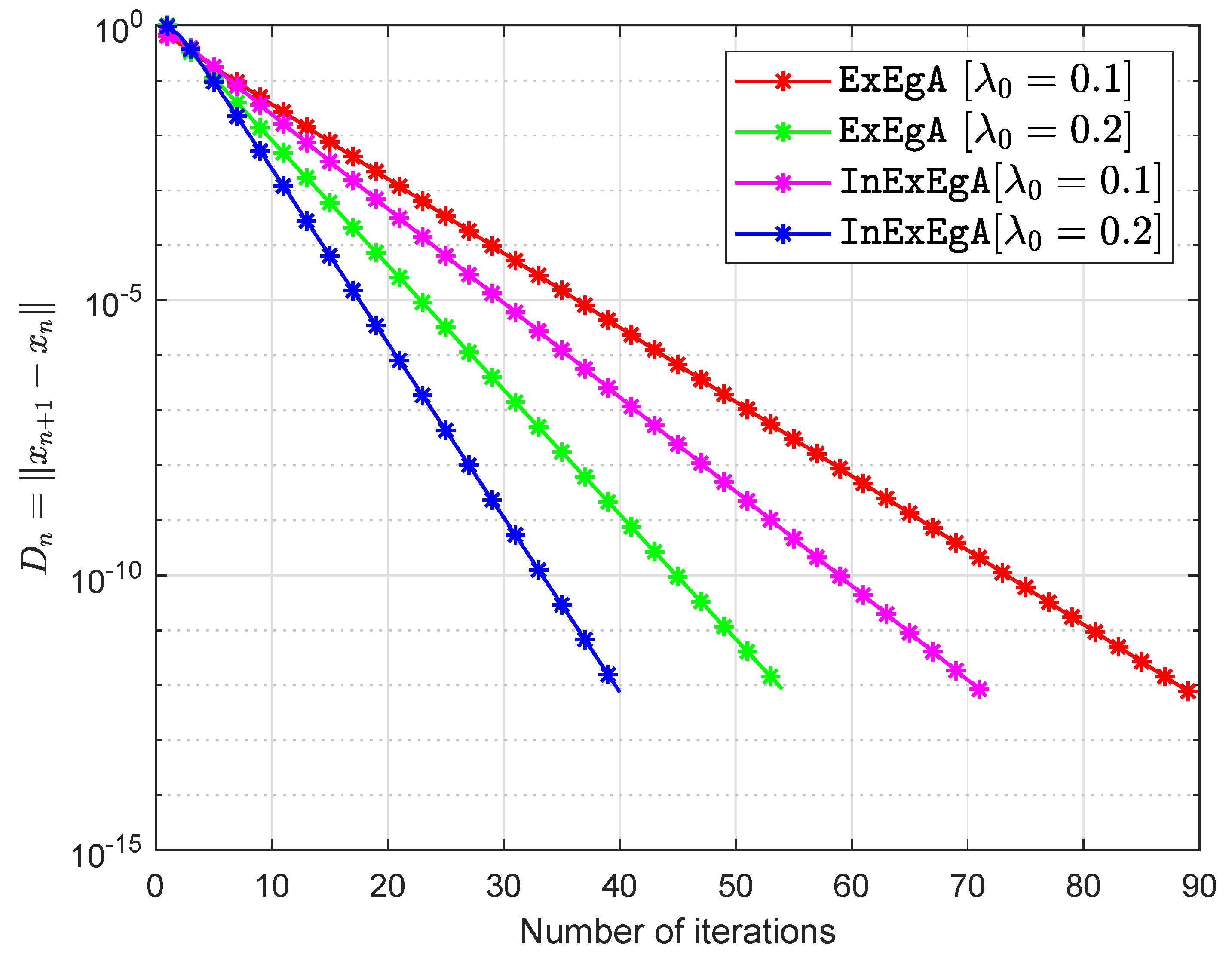
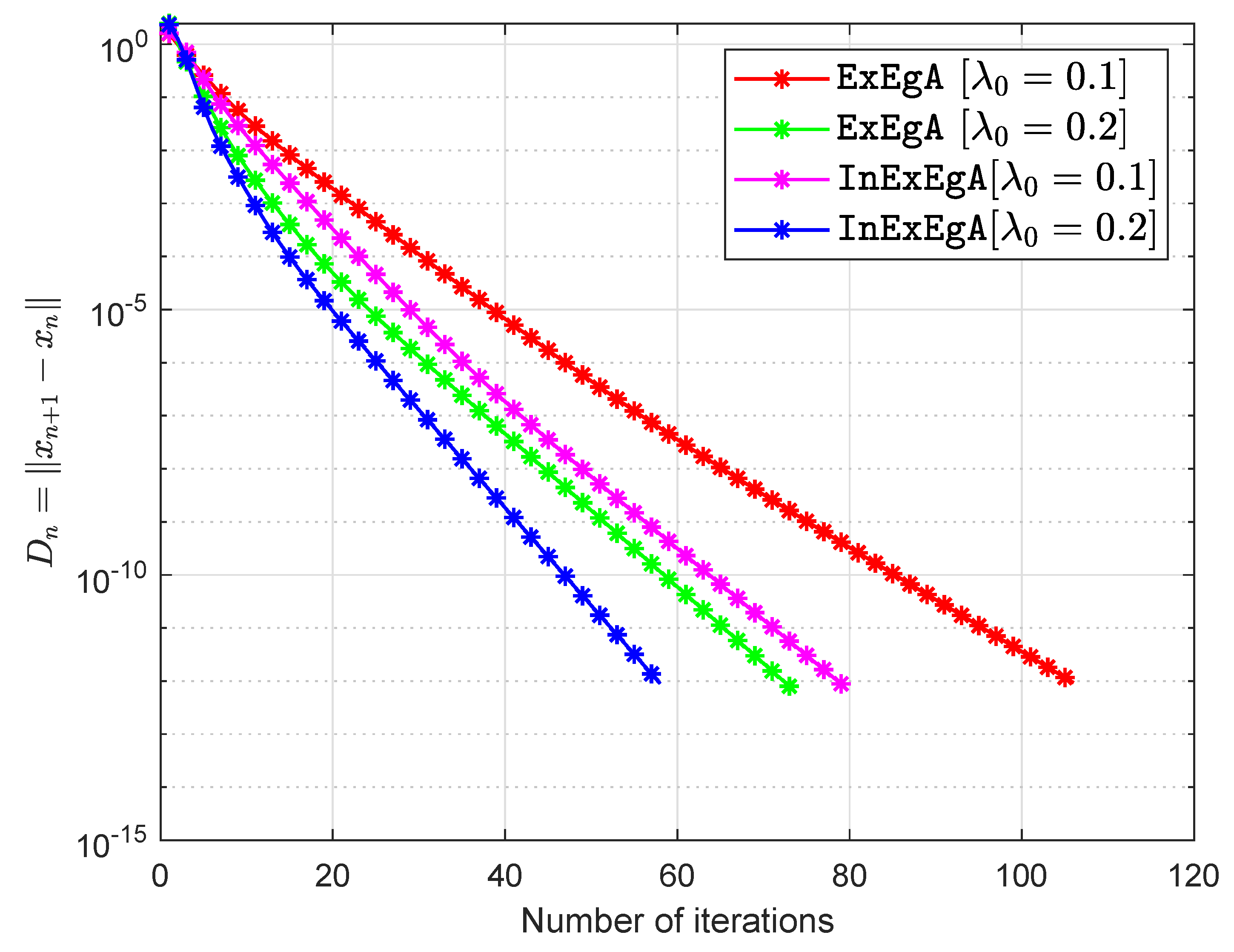
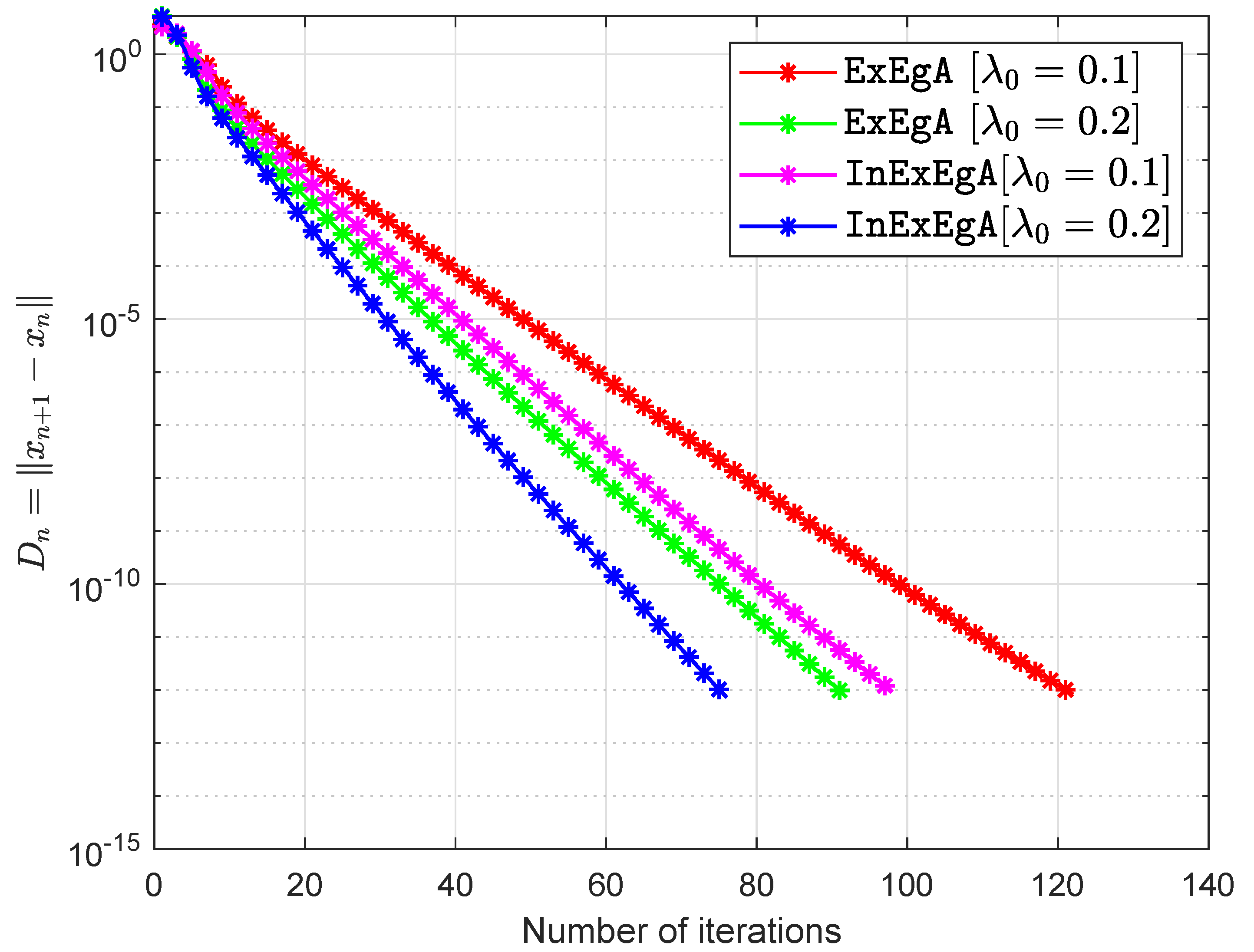
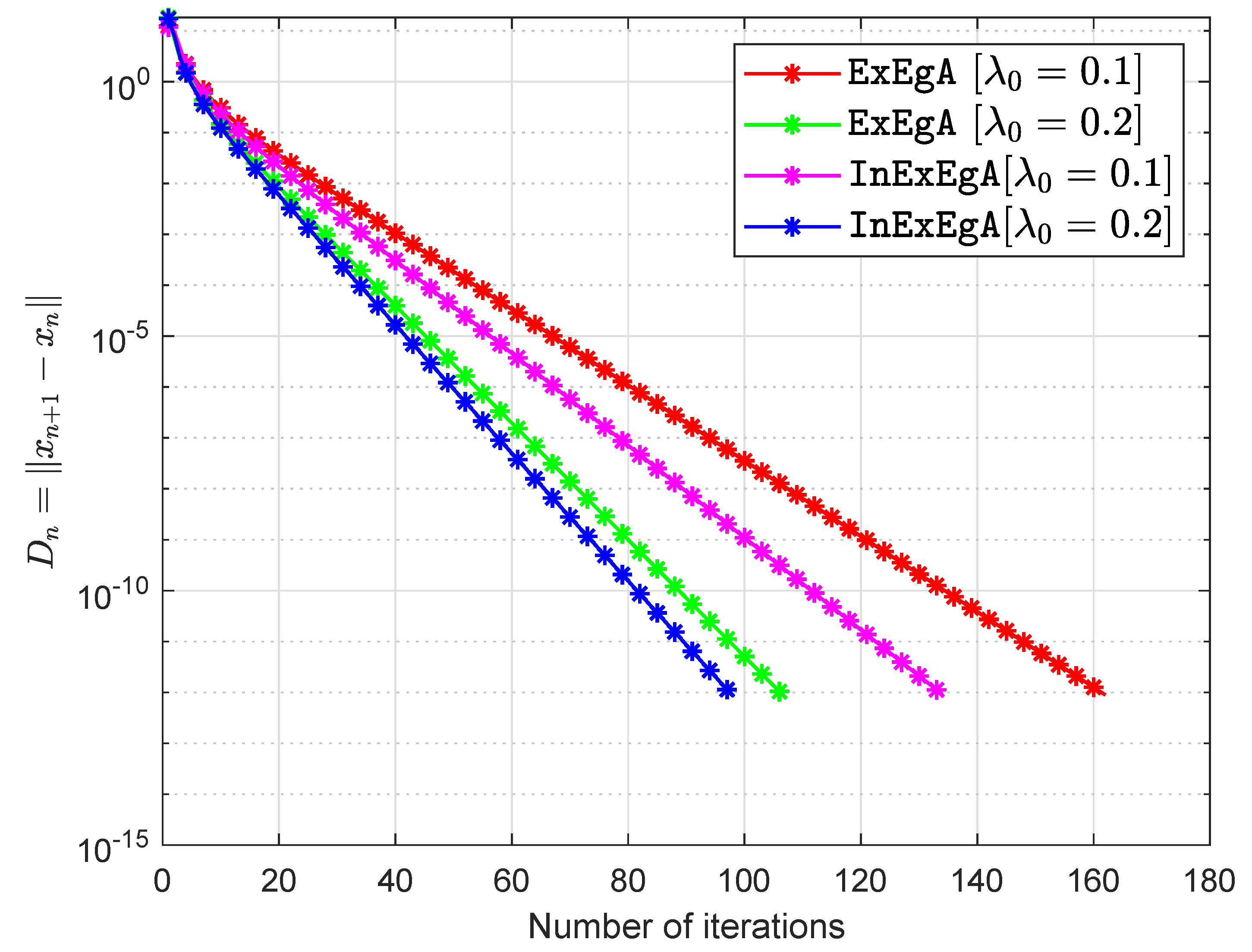
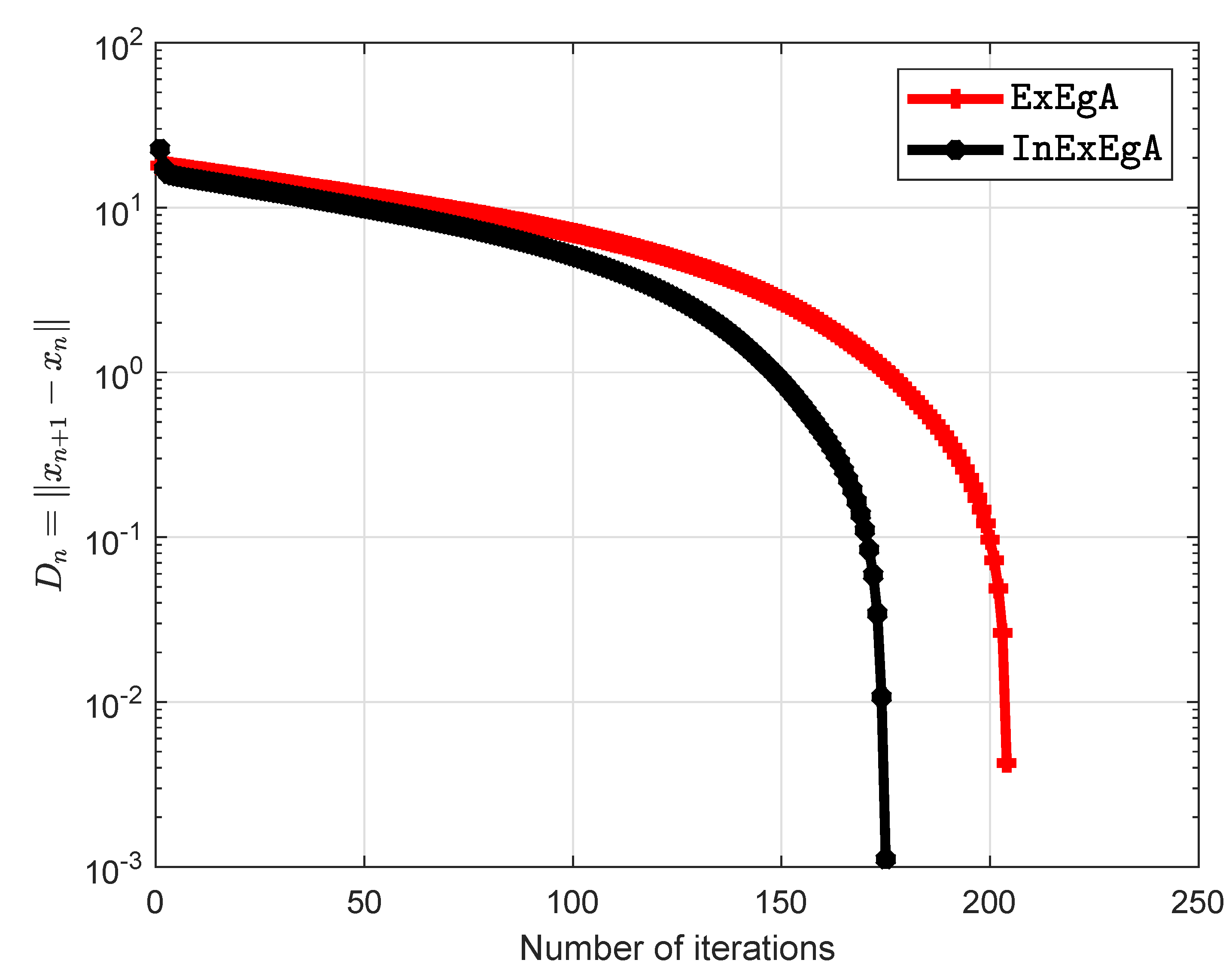
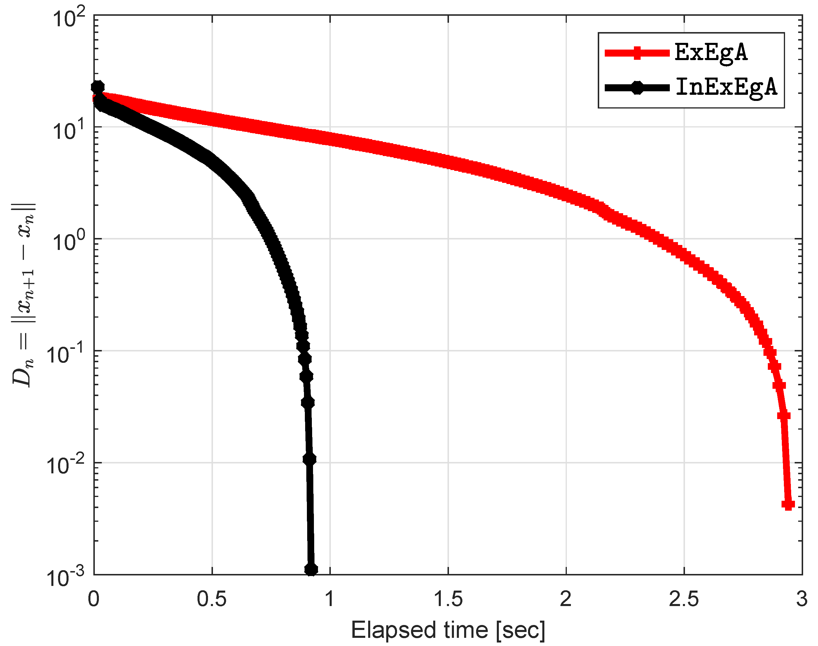
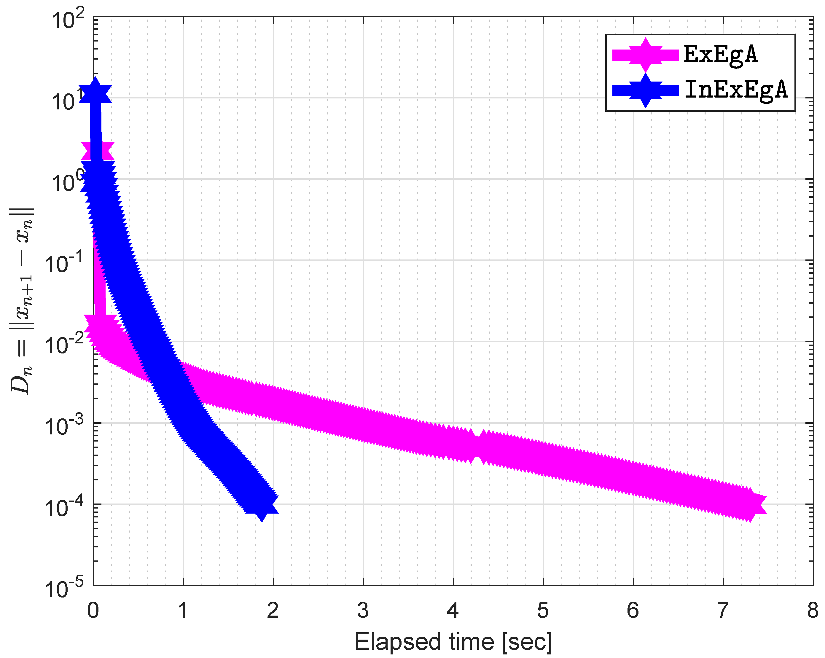
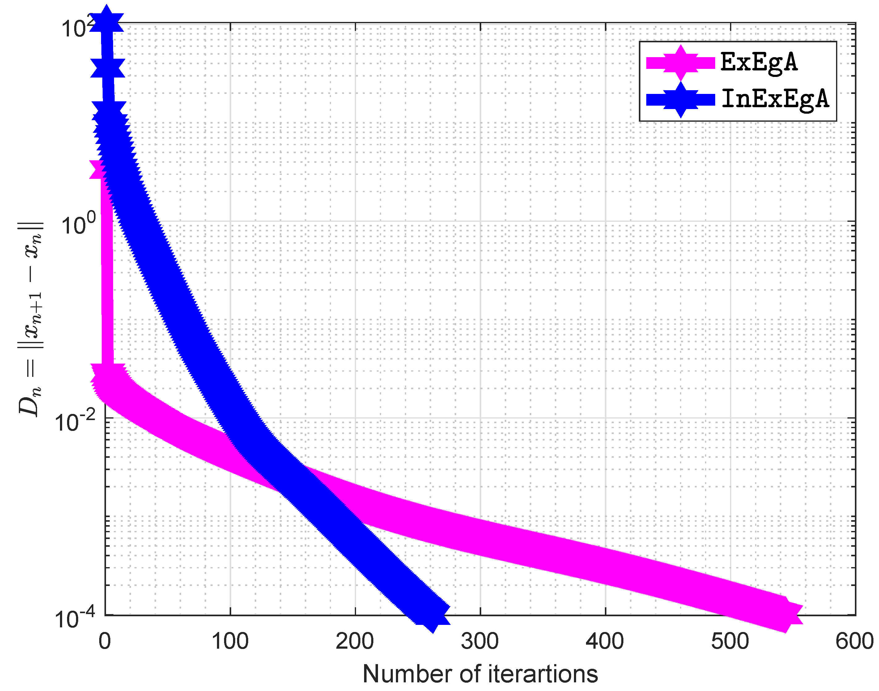
4. Numerical Experiments

For numerical experiments, we analyzed four examples by allowing different dimensions to see the effectiveness of our proposed method. We used the Matlab Quadprog program (https://www.mathworks.com/help/optim/ug/quadprog.html) to solve optimization problems and computed on a (Matlab R2018b) PC Intel(R) Core(TM)i5-6200 CPU @ 2.30GHz 2.40GHz, RAM 8.00 GB.

Example 1.

Assume that there have been n companies that manufacture the same commodities and this model taken as extension of the Nash-Cournot Oligopolistic equilibrium model [36]. Let x correspond to a vector in which every element $x_i$ indicates the amount of the commodity generated by the company i. So, in this case the price function P has been taken the form as $P_i\left(S\right)={\varphi }_i-{\psi }_{i}S,$ where ${\varphi }_i>0,$${\psi }_i>0$ and $S={\sum }_{i=1}^n{x}_i$ is the sum of total commodity generated by all companies. The profit function for each firm i is defined by $F_i\left(x\right)=P_i\left(S\right)x_i-t_i\left(x_i\right)$ where $t_i\left(x_i\right)$ is the value of tax and fee for producing $x_i.$ Suppose that $C_i=[x_i^{min},x_i^{max}]$ is the set of strategies belongs to each firm i and the strategy scheme for the whole model take the form as $C:=C_1\times C_2\times \cdots \times C_n.$ In particular, each organization desires to attain its optimum return by considering that the resulting amount of production is an input parameter and is dependent on the engagement of all the other parties. The methodology frequently managed to work on this type of model primarily concentrates on the well-known Nash equilibrium principle. A point $x^{*}\in C=C_1\times C_2\times \cdots \times C_n$ is an equilibrium point of the above-discussed model if

$$F_i\left(x^{*}\right)\ge F_i\left(x^{*}\left[x_i\right]\right)\forall x_i\in C_i,\forall i=1,2,\cdots ,n,$$

while the vector $x^{*}\left[x_i\right]$ represent the vector get from $x^{*}$ by taking $x_i^{*}$ with $x_i.$ Finally, we take $f(x,y):=\phi (x,y)-\phi (x,x)$ with $\phi (x,y):=-{\sum }_{i=1}^n{F}_i\left(x\left[y_i\right]\right)$ and the problem of finding the Nash equilibrium point of the model can be taken as follows:

$$\mathrm{Find}{x}^{*}\in C\mathrm{such}\mathrm{that}f(x^{*},y)\ge 0,\forall y\in C.$$

It follows from [36,46], the bifunction $f:C\times C\to \mathbb{R}$ could be taken in the following form

$$f(x,y)=\langle Px+Qy+q,y-x\rangle ,$$

while $C\subset {\mathbb{R}}^n$ is defined as

$$C:=\{x\in {\mathbb{R}}^n:-5\le x_i\le 5\}.$$

The matrices $P,Q$ are being taken arbitrary (Choosing two diagonal matrices randomly $A_1$ and $A_2$ with entries from $[0,2]$ and $[-2,0]$ respectively. Two random orthogonal matrices $B_1$ and $B_2$ are able to generate a positive semidefinite matrix $M_1=B_1{A}_1{B}_1^T$ and negative semidefinite matrix $M_2=B_2{A}_2{B}_2^T.$ Finally, set $Q=M_1+M_1^T,$$S=M_2+M_2^T$ and $P=Q-S$) and vector q entries taken from interval $[-n,n]$ (for more details see [36,47]). The starting points are $x_{-1}=x_0={(1,1,\cdots ,1)}^T\in {\mathbb{R}}^n$ and $\mu =0.22,$${\theta }_n=0.20$ with ${\beta }_n=0.85$. Figure 1, Figure 2, Figure 3 and Figure 4 and

Table 1. Example 1: The numerical results for Figure 1, Figure 2, Figure 3 and Figure 4.

			ExEgA		InExEgA
n	${\mathit{\xi }}_0$	TOL	Iter.	CPU(s)	Iter.	CPU(s)
	0.1	${10}^{-12}$	89	0.8725	71	0.5018
5	0.2	${10}^{-12}$	54	0.4895	40	0.2080
	0.1	${10}^{-12}$	106	1.1755	79	0.6562
10	0.2	${10}^{-12}$	73	0.8509	58	0.4067
	0.1	${10}^{-12}$	122	1.5985	98	0.9870
20	0.2	${10}^{-12}$	91	1.0032	76	0.7689
	0.1	${10}^{-12}$	162	2.4567	134	1.4567
50	0.2	${10}^{-12}$	107	1.4356	98	1.0067

demonstrates the numerical performance of Algorithm 1 (InExEgA) comparison with Algorithm 1 (ExEgA) in [16] relative to number of iterations.

Example 2.

Consider the following problem of fractional programming as in [48]:

$$ming\left(x\right)=\frac{x^{T}Qx+a^{T}x+a_0}{b^{T}x+b_0}$$

subject to $x\in C:=\{x\in {\mathbb{R}}^4:b^{T}x+b_0>0\}$ where $a_0=-2,b_0=4$ and

$$Q=\left(\begin{array}{cccc}5& -1& 2& 0\\ -1& 5& -1& 3\\ 2& -1& 3& 0\\ 0& 3& 0& 5\end{array}\right),a=\left(\begin{array}{c}1\\ -2\\ -2\\ 1\end{array}\right),b=\left(\begin{array}{c}2\\ 1\\ 1\\ 0\end{array}\right).$$

It is easy to verify that Q is symmetric and positive definite in ${\mathbb{R}}^4$ and consequently g is pseudoconvex on C. We minimize g over $C:=\{x\in {\mathbb{R}}^4:1\le x_i\le 10,i=1,2,3,4\}$ by using both algorithms with bifunction $f(x,y)=\langle G\left(x\right),y-x\rangle$ on $C\times C$ to $\mathbb{R}$ with unknown Lipschitz constants where

$$G\left(x\right):=▽g\left(x\right)=\frac{((b^{T}x+b_0)(2Qx+a)-b(x^{T}Qx+a^{T}x+a_0))}{{(b^{T}x+b_0)}^2}.$$

This problem has a unique solution $x^{*}={(1,1,1,1)}^T\in C.$ Choose initial points are $x_{-1}=x_0={(1,1,1,1)}^T\in {\mathbb{R}}^4$ and $\mu =0.22,$ ${\theta }_n=0.20,$ ${\beta }_n=0.85,$ ${\xi }_0=0.5$. Figure 5 and Figure 6 demonstrates the numerical performance of Algorithm 1 (InExEgA) comparison with Algorithm 1 (ExEgA) in [16] in term of number of iterations and elapsed time respectively.

Example 3.

Let the bifunction f define on the convex set C as

$$f(x,y)=〈(B{B}^T+S+D)x,y-x〉,$$

where B is an $m\times m$ matrix, S is an $m\times m$ skew-symmetric matrix, D is an $m\times m$ diagonal matrix, whose diagonal entries are nonnegative. The feasible set $C\subset {\mathbb{R}}^m$ is closed and convex and defined as

$$C=\{x\in {\mathbb{R}}^m:Ax\le b\},$$

while A is an $l\times m$ matrix and b is a nonnegative vector. It is clear that bifunction f is monotone and its Lipschitz-type constants are $c_1=c_2=\frac{\parallel B{B}^T+S+D\parallel }{2}.$ The initial points are $x_{-1}=x_0={(1,1,\cdots ,1)}^T\in {\mathbb{R}}^n$ and $\mu =0.22,$ ${\theta }_n=0.20$ with ${\beta }_n=0.85$. Figure 7, Figure 8, Figure 9, Figure 10, Figure 11 and Figure 12 and

Table 2. Example 3: The numerical results for Figure 7, Figure 8, Figure 9, Figure 10, Figure 11 and Figure 12.

			ExEgA		InExEgA
n	${\mathit{\xi }}_0$	TOL	Iter.	CPU(s)	Iter.	CPU(s)
5	0.5	${10}^{-4}$	205	7.2979	131	1.8722
10	0.5	${10}^{-4}$	544	23.0891	262	4.6898
20	0.5	${10}^{-4}$	1562	65.7050	1084	23.1766

demonstrates the numerical performance of Algorithm 1 comparison with Algorithm 1 in [16] in term of number of iterations and elapsed time in seconds.

Example 4.

Consider a bifunction $f:C\times C\to \mathbb{R}$ defined by

$$f(x,y)=\langle F\left(x\right),y-x\rangle ,$$

with unknown Lipschitz constants $c_1,c_2$ and $C=\{x\in {\mathbb{R}}^4:1\le x_i\le 5,i=1,2,3,4\}$ and

$$F\left(x\right)=\left(\begin{array}{c}{x}_1+x_2+x_3+x_4-4x_2{x}_3{x}_4\\ x_1+x_2+x_3+x_4-4x_1{x}_3{x}_4\\ x_1+x_2+x_3+x_4-4x_1{x}_2{x}_4\\ x_1+x_2+x_3+x_4-4x_1{x}_2{x}_3\end{array}\right).$$

The initial values are $x_{-1}=x_0={(1,1,1,1)}^T\in {\mathbb{R}}^n$ and $\mu =0.22,$ ${\theta }_n=0.20$ with ${\beta }_n=0.85$. Figure 13 and Figure 14 demonstrates the numerical performance of Algorithm 1 comparison with Algorithm 1 in [16].

5. Conclusions

The paper proposed an inertial extragradient-like approach to addressing the problem of equilibrium of a pseudomonotone bifunction with a Lipschitz-like condition. A stepsize rule has been presented that does not depend on the Lipschitz-type constant information. Several experimental studies have been reported to demonstrate the numerical behavior of our method and compare it with other methods. Such numerical experiments indicate that inertial influences normally extend the performance of iterative sequences in this sense.

References

1. Blum, E. From optimization and variational inequalities to equilibrium problems. Math. Student 1994, 63, 123–145. [Google Scholar]
2. Muu, L.D.; Oettli, W. Convergence of an adaptive penalty scheme for finding constrained equilibria. Nonlinear Anal. Theory Methods Appl. 1992, 18, 1159–1166. [Google Scholar] [CrossRef]
3. Facchinei, F.; Pang, J.S. Finite-Dimensional Variational Inequalities and Complementarity Problems; Springer Science & Business Media: Berlin, Germany, 2007. [Google Scholar]
4. Fan, K. A Minimax Inequality and Applications, Inequalities III; Shisha, O., Ed.; Academic Press: New York, NY, USA, 1972. [Google Scholar]
5. Hieu, D.V. Projected subgradient algorithms on systems of equilibrium problems. Optim. Lett. 2017, 12, 551–566. [Google Scholar] [CrossRef]
6. Scheimberg, S.; Santos, P. A relaxed projection method for finite-dimensional equilibrium problems. Optimization 2011, 60, 1193–1208. [Google Scholar] [CrossRef]
7. Muu, L.D.; Quoc, T.D. Regularization Algorithms for Solving Monotone Ky Fan Inequalities with Application to a Nash-Cournot Equilibrium Model. J. Optim. Theory Appl. 2009, 142, 185–204. [Google Scholar] [CrossRef]
8. ur Rehman, H.; Kumam, P.; Argyros, I.K.; Deebani, W.; Kumam, W. Inertial Extra-Gradient Method for Solving a Family of Strongly Pseudomonotone Equilibrium Problems in Real Hilbert Spaces with Application in Variational Inequality Problem. Symmetry 2020, 12, 503. [Google Scholar] [CrossRef] [Green Version]
9. Moudafi, A. Proximal point algorithm extended to equilibrium problems. J. Nat. Geometry 1999, 15, 91–100. [Google Scholar]
10. Flåm, S.D.; Antipin, A.S. Equilibrium programming using proximal-like algorithms. Math. Progr. 1996, 78, 29–41. [Google Scholar] [CrossRef]
11. Quoc, T.D.; Anh, P.N.; Muu, L.D. Dual extragradient algorithms extended to equilibrium problems. J. Glob. Optim. 2011, 52, 139–159. [Google Scholar] [CrossRef]
12. Lyashko, S.I.; Semenov, V.V. A New Two-Step Proximal Algorithm of Solving the Problem of Equilibrium Programming. In Optimization and Its Applications in Control and Data Sciences; Springer International Publishing: Berlin, Germany, 2016; pp. 315–325. [Google Scholar] [CrossRef]
13. ur Rehman, H.; Kumam, P.; Cho, Y.J.; Yordsorn, P. Weak convergence of explicit extragradient algorithms for solving equilibirum problems. J. Inequalities Appl. 2019, 2019. [Google Scholar] [CrossRef]
14. Anh, P.N.; Hai, T.N.; Tuan, P.M. On ergodic algorithms for equilibrium problems. J. Glob. Optim. 2015, 64, 179–195. [Google Scholar] [CrossRef]
15. ur Rehman, H.; Kumam, P.; Argyros, I.K.; Shutaywi, M.; Shah, Z. Optimization Based Methods for Solving the Equilibrium Problems with Applications in Variational Inequality Problems and Solution of Nash Equilibrium Models. Mathematics 2020, 8, 822. [Google Scholar] [CrossRef]
16. Hieu, D.V.; Quy, P.K.; Vy, L.V. Explicit iterative algorithms for solving equilibrium problems. Calcolo 2019, 56. [Google Scholar] [CrossRef]
17. Hieu, D.V. New extragradient method for a class of equilibrium problems in Hilbert spaces. Appl. Anal. 2017, 97, 811–824. [Google Scholar] [CrossRef]
18. ur Rehman, H.; Kumam, P.; Je Cho, Y.; Suleiman, Y.I.; Kumam, W. Modified Popov’s explicit iterative algorithms for solving pseudomonotone equilibrium problems. Optim. Methods Softw. 2020, 1–32. [Google Scholar] [CrossRef]
19. ur Rehman, H.; Kumam, P.; Abubakar, A.B.; Cho, Y.J. The extragradient algorithm with inertial effects extended to equilibrium problems. Comput. Appl. Math. 2020, 39. [Google Scholar] [CrossRef]
20. ur Rehman, H.; Kumam, P.; Kumam, W.; Shutaywi, M.; Jirakitpuwapat, W. The Inertial Sub-Gradient Extra-Gradient Method for a Class of Pseudo-Monotone Equilibrium Problems. Symmetry 2020, 12, 463. [Google Scholar] [CrossRef] [Green Version]
21. Hieu, D.V. Convergence analysis of a new algorithm for strongly pseudomontone equilibrium problems. Numer. Algorithms 2017, 77, 983–1001. [Google Scholar] [CrossRef]
22. Hieu, D.V.; Strodiot, J.J. Strong convergence theorems for equilibrium problems and fixed point problems in Banach spaces. J. Fixed Point Theory Appl. 2018, 20. [Google Scholar] [CrossRef]
23. ur Rehman, H.; Kumam, P.; Argyros, I.K.; Alreshidi, N.A.; Kumam, W.; Jirakitpuwapat, W. A Self-Adaptive Extra-Gradient Methods for a Family of Pseudomonotone Equilibrium Programming with Application in Different Classes of Variational Inequality Problems. Symmetry 2020, 12, 523. [Google Scholar] [CrossRef] [Green Version]
24. Hieu, D.V.; Gibali, A. Strong convergence of inertial algorithms for solving equilibrium problems. Optim. Lett. 2019. [Google Scholar] [CrossRef]
25. Abubakar, J.; Kumam, P.; ur Rehman, H.; Ibrahim, A.H. Inertial Iterative Schemes with Variable Step Sizes for Variational Inequality Problem Involving Pseudomonotone Operator. Mathematics 2020, 8, 609. [Google Scholar] [CrossRef]
26. Abubakar, J.; Sombut, K.; ur Rehman, H.; Ibrahim, A.H. An Accelerated Subgradient Extragradient Algorithm for Strongly Pseudomonotone Variational Inequality Problems. Thai J. Math. 2019, 18, 166–187. [Google Scholar]
27. ur Rehman, H.; Kumam, P.; Shutaywi, M.; Alreshidi, N.A.; Kumam, W. Inertial Optimization Based Two-Step Methods for Solving Equilibrium Problems with Applications in Variational Inequality Problems and Growth Control Equilibrium Models. Energies 2020, 13, 3292. [Google Scholar] [CrossRef]
28. Iusem, A.N.; Sosa, W. On the proximal point method for equilibrium problems in Hilbert spaces. Optimization 2010, 59, 1259–1274. [Google Scholar] [CrossRef]
29. Martinet, B. Brève communication. Régularisation d’inéquations variationnelles par approximations successives. Revue Française D’inf. Rech. Opérationnelle. Série Rouge 1970, 4, 154–158. [Google Scholar] [CrossRef] [Green Version]
30. Rockafellar, R.T. Monotone operators and the proximal point algorithm. SIAM J. Control Optim. 1976, 14, 877–898. [Google Scholar] [CrossRef] [Green Version]
31. Konnov, I. Application of the Proximal Point Method to Nonmonotone Equilibrium Problems. J. Optim. Theory Appl. 2003, 119, 317–333. [Google Scholar] [CrossRef]
32. Cohen, G. Auxiliary problem principle and decomposition of optimization problems. J. Optim. Theory Appl. 1980, 32, 277–305. [Google Scholar] [CrossRef]
33. Cohen, G. Auxiliary problem principle extended to variational inequalities. J. Optim. Theory Appl. 1988, 59, 325–333. [Google Scholar] [CrossRef]
34. Mastroeni, G. On Auxiliary Principle for Equilibrium Problems. In Nonconvex Optimization and Its Applications; Springer: Berlin, Germany, 2003; pp. 289–298. [Google Scholar] [CrossRef]
35. Korpelevich, G. The extragradient method for finding saddle points and other problems. Matecon 1976, 12, 747–756. [Google Scholar]
36. Quoc Tran, D.; Le Dung, M.N.V.H. Extragradient algorithms extended to equilibrium problems. Optimization 2008, 57, 749–776. [Google Scholar] [CrossRef]
37. Censor, Y.; Gibali, A.; Reich, S. The Subgradient Extragradient Method for Solving Variational Inequalities in Hilbert Space. J. Optim. Theory Appl. 2010, 148, 318–335. [Google Scholar] [CrossRef] [PubMed] [Green Version]
38. Goebel, K.; Reich, S. Uniform convexity, Hyperbolic Geometry, and Nonexpansive Mappings. 1984. Available online: https://www.researchgate.net/publication/248772020_Uniform_Convexity_Hyperbolic_Geometry_and_Nonexpansive_Mappings (accessed on 10 June 2020).
39. Minty, G.J. Monotone (nonlinear) operators in Hilbert space. Duke Math. J. 1962, 29, 341–346. [Google Scholar] [CrossRef]
40. Karamardian, S.; Schaible, S. Seven kinds of monotone maps. J. Optim. Theory Appl. 1990, 66, 37–46. [Google Scholar] [CrossRef]
41. Bianchi, M.; Schaible, S. Generalized monotone bifunctions and equilibrium problems. J. Optim. Theory Appl. 1996, 90, 31–43. [Google Scholar] [CrossRef]
42. Tiel, J.V. Convex Analysis: An Introductory Text, 1st ed.; Wiley: New York, NY, USA, 1984. [Google Scholar]
43. Heinz, H.; Bauschke, P.L.C.A. Convex Analysis and Monotone Operator Theory in Hilbert Spaces, 2nd ed.; CMS Books in Mathematics; Springer: Berlin, Germany, 2017. [Google Scholar]
44. Attouch, F.A.H. An Inertial Proximal Method for Maximal Monotone Operators via Discretization of a Nonlinear Oscillator with Damping. Set-Valued Var. Anal. 2001, 9, 3–11. [Google Scholar] [CrossRef]
45. Opial, Z. Weak convergence of the sequence of successive approximations for nonexpansive mappings. Bull. Amer. Math. Soc. 1967, 73, 591–598. [Google Scholar] [CrossRef] [Green Version]
46. Hieu, D.V. Parallel extragradient-proximal methods for split equilibrium problems. Math. Modell. Anal. 2016, 21, 478–501. [Google Scholar] [CrossRef]
47. ur Rehman, H.; Pakkaranang, N.; Hussain, A.; Wairojjana, N. A modified extra-gradient method for a family of strongly pseudomonotone equilibrium problems in real Hilbert spaces. J. Math. Comput. Sci. 2020, 22, 38–48. [Google Scholar] [CrossRef]
48. Hu, X.; Wang, J. Solving Pseudomonotone Variational Inequalities and Pseudoconvex Optimization Problems Using the Projection Neural Network. IEEE Trans. Neural Netw. 2006, 17, 1487–1499. [Google Scholar] [CrossRef] [PubMed] [Green Version]
Figure 1. Algorithm 1 comparison with Algorithm 1 in [16] in term of iterations when n = 5 .
Mathematics 08 01165 g001
Figure 2. Algorithm 1 comparison with Algorithm 1 in [16] in term of iterations when n = 10 .
Mathematics 08 01165 g002
Figure 3. Algorithm 1 comparison with Algorithm 1 in [16] in term of iterations when n = 20 .
Mathematics 08 01165 g003
Figure 4. Algorithm 1 comparison with Algorithm 1 in [16] in term of iterations when n = 50 .
Mathematics 08 01165 g004
Figure 5. Algorithm 1 comparison with Algorithm 1 in [16] and number of iterations are 204 and 175 respectively.
Mathematics 08 01165 g005
Figure 6. Algorithm 1 comparison with Algorithm 1 in [16] and elapsed time in seconds are 2.9404 and 0.9194 respectively.
Mathematics 08 01165 g006
Figure 7. Algorithm 1 comparison with Algorithm 1 in [16] when m = 5 .
Mathematics 08 01165 g007
Figure 8. Algorithm 1 comparison with Algorithm 1 in [16] when m = 5 .
Mathematics 08 01165 g008
Figure 9. Algorithm 1 comparison with Algorithm 1 in [16] when m = 10 .
Mathematics 08 01165 g009
Figure 10. Algorithm 1 comparison with Algorithm 1 in [16] when m = 10 .
Mathematics 08 01165 g010
Figure 11. Algorithm 1 comparison with Algorithm 1 in [16] when m = 20 .
Mathematics 08 01165 g011
Figure 12. Algorithm 1 comparison with Algorithm 1 in [16] when m = 20 .
Mathematics 08 01165 g012
Figure 13. Algorithm 1 comparison with Algorithm 1 in [16] and number of iterations are 108 and 49 respectively.
Mathematics 08 01165 g013
Figure 14. Algorithm 1 comparison with Algorithm 1 in [16] and elapsed time in seconds are 1.3294 and 0.1701 respectively.
Mathematics 08 01165 g014