Detection of Cropland Change Using Multi-Harmonic Based Phenological Trajectory Similarity

Abstract

Accurate information on cropland changes is critical for food production and security, sustainable cropland management, and global change studies. The common change detection methods bi-temporal based, using remotely sensed imagery easily generate pseudo changes due to phenological or seasonal differences. Cropland exhibits a distinctive phenological trajectory that has strong periodic characteristics and seasonal paths. This paper proposes the use of phenological trajectory similarity to search for the overall changes between two time-series images instead of single change events between two dates of imagery. Due to the complex spectral–temporal characteristic of cropland, a phenological trajectory was constructed using a multi-harmonic model for capturing intra-annual variations. Then, phenological trajectory similarity was measured using coefficient vector difference (CVD), and used for detecting change/no-change areas when considering both the amplitude and phase difference. Finally, instead of the traditional classification method based on original images, we used the coefficient ratio vector (CRV) as the input for change type discrimination. The distance between the coefficient ratio vector (CRV) of the change pixel and of the reference change type was calculated to identify the exactly changed types. The performance of this proposed approach was tested using two sets of Landsat time-series images from 2010 and 2015. Moreover, the change area detection results of three other methods, namely, the continuous change detection and classification (CCDC), change vector analysis (CVA), and post-classification comparison (PCC), were also calculated for comparison and analysis. The results indicated that the proposed approach acquired the highest accuracy with an overall accuracy of 98.58% and a kappa coefficient of 0.82, which demonstrated that the method provides the capacity to detect real changes and estimate pseudo changes caused by season differences.

1. Introduction

Cropland is the basic resource and condition of human existence, and its quantity and quality are an important basis for ensuring global food production security [1]. Cropland changes not only directly threaten the survival and development of mankind, food production, and security, but also affect the biogeochemical cycles, global warming, and lead to environmental problems [2,3,4]. However, large areas of cropland have been shrinking over the past decades due to rapid urbanization and forest plantations [5]. Therefore, timely, accurate, and cost-effective cropland change detection is critical for more effective policy making, yield estimation, and sustainable cropland management practices [6,7,8,9].

Remote sensing has proven to be useful for mapping and characterizing cropland information [10,11]. A variety of change detection methods utilizing remote sensing data have been developed for detecting changes [12,13,14]. The widely used methods including image differencing, change vector analysis (CVA), and post-classification comparison (PCC), are based on a bi-temporal strategy, which is quite simple and straightforward [15,16,17]. However, since cropland changes dramatically with the season shifts, pseudo changes caused by phenological differences are more likely to be produced [18,19]. Recently, time series analysis has been proven to be superior to the bi-temporal methods for capturing land cover change, since it significantly reduces the impacts of seasonal differences and interference noises [20,21,22]. Accordingly, many algorithms based on time-series analysis have been proposed for assessing change. For example, the Landsat-based Detection of Trends in Disturbance and Recovery (Landtrendr) proposed by Kennedy et al., (2010) detected an abrupt forest disturbance using a temporal segmentation algorithm [23]. The Breaks for Additive Seasonal and Trend (BFAST) algorithm developed by Verbesselt et al., (2010) is capable of capturing multiple breakpoint changes by estimating time and magnitude of changes occurring within the seasonal or trend components [24,25,26]. The Continuous Change Detection and Classification (CCDC) estimated the trend of the time-series by using harmonic models and utilized this trend to characterize multiple changes, including abrupt [27].

Although these approaches are very effective in identifying abrupt or gradual changes, they only focused on the detection of forest disturbance and urban expansion, while neglecting agricultural or cropland variations [28,29]. This is mainly due to the fact that the cropland may possess not only more complicated spectral features but also more dynamic temporal characteristics due to the discrepancies between categories, phenology, and growth stage [30,31]. Therefore, the existing methods may be invalid for cropland change detection. To fully capture cropland changes, it is necessary to excavate more temporal information (e.g., phenological information).

Fortunately, cropland phenology is a temporal feature that describes the seasonal growth and dynamic development of cropland, which is primarily featured by the obvious time phases of sowing, emergence, growing, ripening, and harvesting. A growing number of studies have focused on utilizing remote sensing data to extract phenology information [32,33,34]. However, most of them mainly focused on the extraction of key phenological parameters, such as the start of the growing season and the end of the season without considering the overall change of phenological characteristics, namely changes in phenology trajectory. Generally, phenological trajectory can be derived from the function model fitting time-series data [35,36]. However, most mathematical models (e.g., logistic model, Gaussian model, and the simple harmonic model) for fitting phenological trajectory have mainly focused on a single growth or senescence cycle that natural vegetation types possess [37,38]. In fact, cropland may present a more complex phenology cycle than natural vegetation, such as double- or triple-crop patterns within a year. Therefore, the existing models fail to fully describe and capture the phenological trajectory of cropland.

In this paper, we propose a new method based on phenological trajectory similarity to solve the issue of pseudo changes caused by phenological differences. The basic idea of the proposed method is that we search for the overall changes between two phenological trajectories instead of exploiting single change events between two dates of imagery. Our method relies on a multi-harmonic model that remarkably matches VI time series due to its periodic changes and season paths. Although most studies mainly utilize the Normalized Difference Vegetation Index (NDVI) time series to capture phenological changes [39,40], the Enhanced Vegetation Index (EVI) still has a higher sensitivity than the NDVI in dense vegetation areas. For this study, we define ‘phenological trajectory’ as the fitted curve through the EVI time series of one year. The objectives of this study are thus (1) to establish a multi-harmonic model to fully capture phenological changes under different cropping patterns, and (2) to test the robustness and performance of the proposed method using Landsat time-series data of Shandong Province, China.

2. Methodology

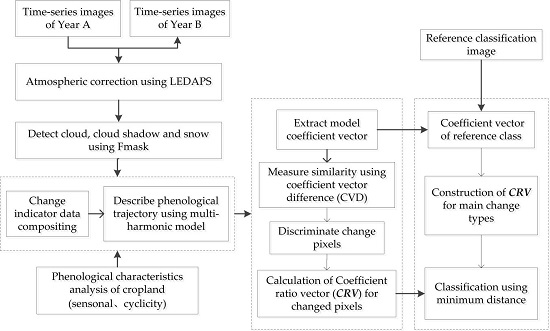
The core of our approach is that we designate finding comprehensive changes between two time-series trajectories rather than searching for the single change events between two dates of imagery. However, image preprocessing is prerequisite for change detection. In this paper, the Landsat Ecosystem Disturbance Adaptive Processing System (LEDAPS) algorithm was used for converting DN to surface reflectance [41], and the Function of mask (Fmask) was use for detecting cloud and cloud shadows. The detailed preprocessing procedure is described in Section 3 [42]. The main body of the proposed method can be split into three parts (Figure 1). First, a multi-harmonic model is established to describe phenological changes for different cropping patterns. Second, based on the phenological trajectory of the pixels, the model coefficient vector difference (CVD) is designed to measure similarity in order to detect change/no-change areas. Third, the coefficient ratio vector (CRV) of reference changed types and of changed pixels is calculated, respectively. Then the change type is discriminated by the minimum distance of the CRV.

2.1. Phenological Trajectory Description Using the Multi-Harmonic Model

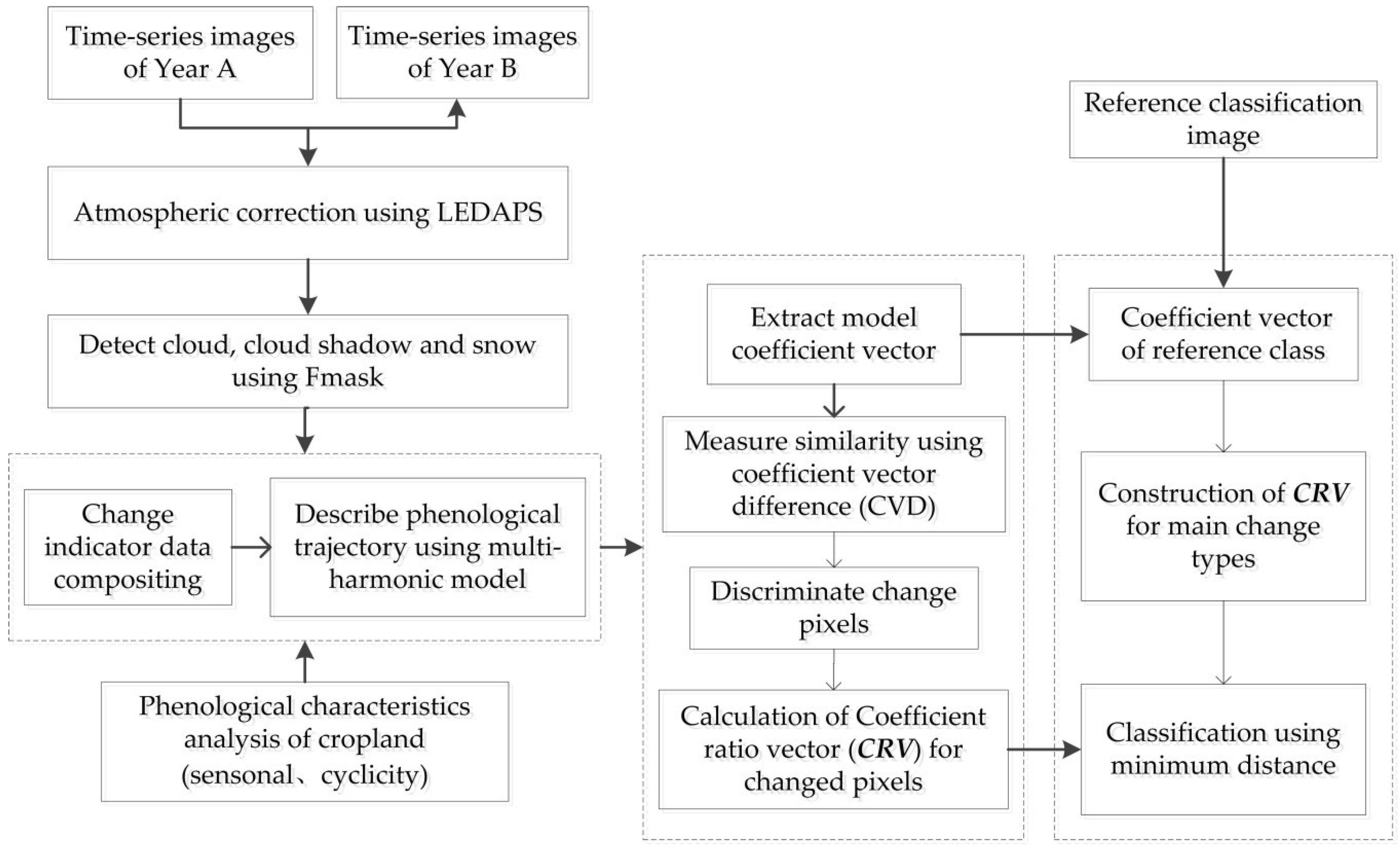
Numerous models have been applied to fit vegetation index (VI) time series for land cover change analysis, such as the local asymmetric Gaussian function (AG), the double logistic (DL), and the harmonic model [43]. Recently, de Beurs and Henebry (2010) presented 12 existing spatio-temporal methods to estimate phenological parameters, and Atkinson et al., (2012) surveyed four time-series models to smooth time-series vegetation index data [44,45]. However, each model has its own advantages and disadvantages, and the choice of model needs to be based on the land cover type. Figure 2 presents the fitting results from three models, the AG, DL, and harmonic model. However, AG and DL are unable to accurately match different waveforms and capture growing season variations as they are always adapted to the upper envelope of the time series. Because the annual phenology of cropland has periodic changes and season paths, the harmonic model remarkably matches the intra-annual VI time series. Moreover, the harmonic model is capable of decomposing a noise-affected time series into periodic signals in the frequency domain, each defined by unique amplitude and phase values [46].

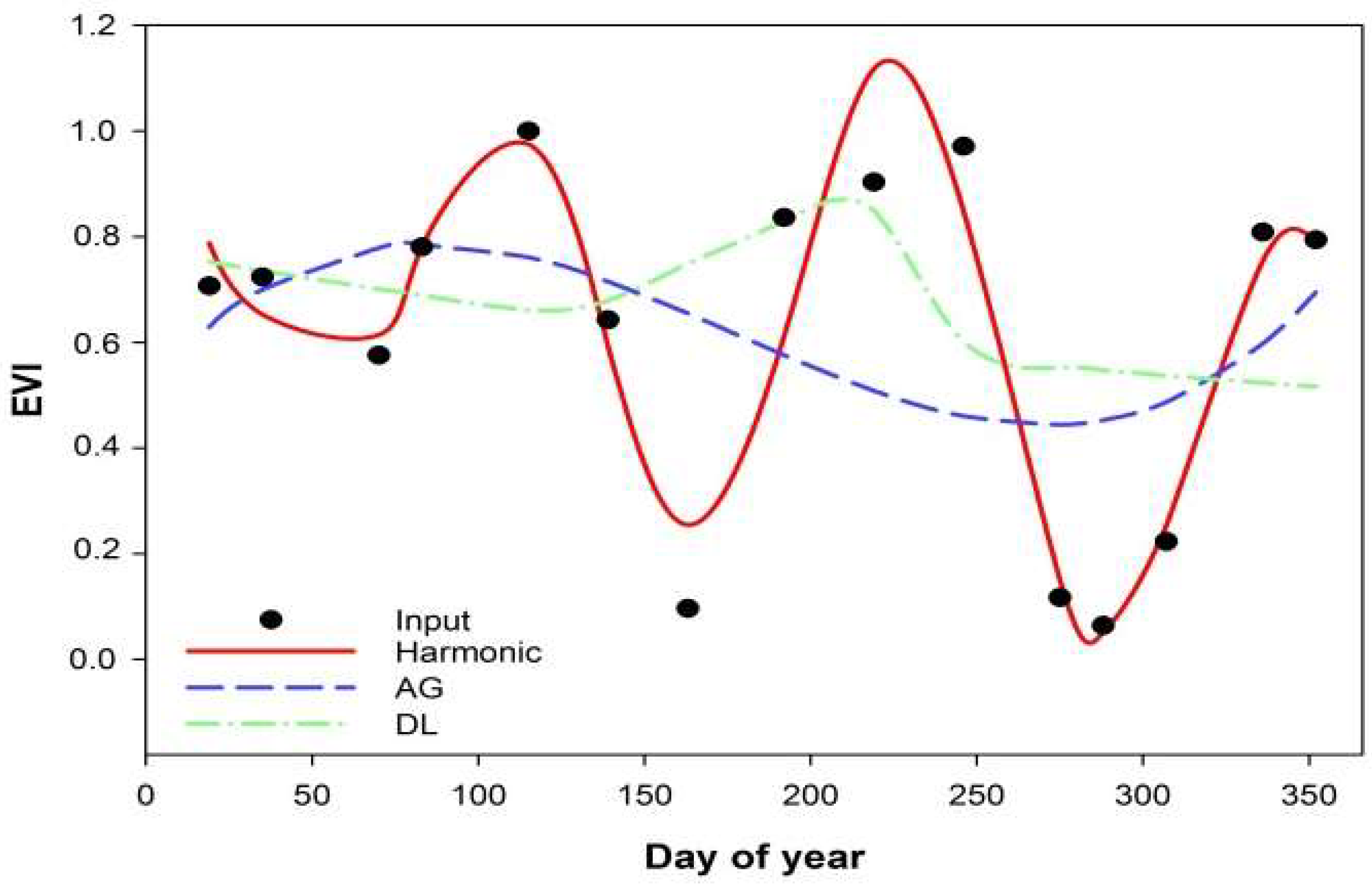
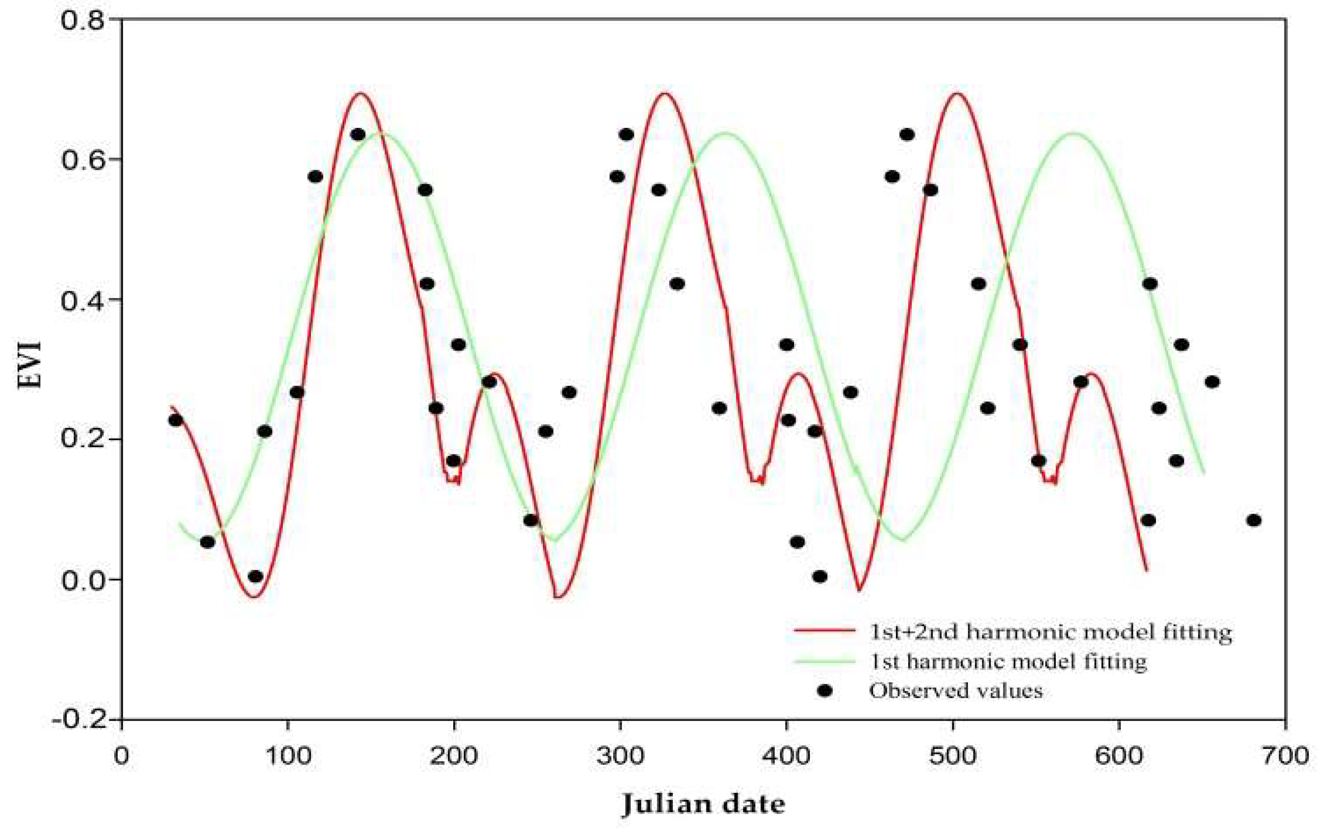
Recently, the continuous change detection and classification (CCDC) algorithm proposed by Zhu and Woodcock (2014) applied simple harmonic model (first order) to predict all land cover types by using all available Landsat images. The simple harmonic model is often not satisfactory for the complex shape of phenological dynamics that has more intra-annual variation, and phenological trajectory description therefore requires high frequency terms for full fitting. Figure 3 shows the phenological trajectory of cropland collected from the Landsat OLI time-series image in 2015, and illustrates the fitting results by including different components of the harmonic model.

In this paper, the multi-harmonic model including the first- and second-order harmonic, was used for describing phenological trajectory. The second harmonic is capable of capturing the detailed phenology of the biannual signal. Moreover, the harmonic model separates components of the time series into different frequency domains. Therefore, the lower-order harmonics (mainly refer to first and second harmonics) accounts for the majority of the VI time series variance while the higher-order components include substantial noise. The multi-harmonic model we adopted is described as follows:

$$\widehat{\mathrm{VI}}\left(\mathrm{t}\right)={\mathrm{a}}_0+{\mathrm{a}}_1\cos \left(\frac{2\mathsf{\pi }}{\mathrm{T}}\mathrm{t}\right)+{\mathrm{b}}_1\sin \left(\frac{2\mathsf{\pi }}{\mathrm{T}}\mathrm{t}\right)+{\mathrm{a}}_2\cos \left(\frac{2\mathsf{\pi }}{0.5\mathrm{T}}\mathrm{t}\right)+{\mathrm{b}}_2\sin \left(\frac{2\mathsf{\pi }}{0.5\mathrm{T}}\mathrm{t}\right)$$

(1)

where

• ${\mathrm{a}}_0$ is the coefficient of the overall value for the vegetation index;
• ${\mathrm{a}}_1{ \mathrm{and} \mathrm{b}}_1$ capture intra-annual change for the vegetation index;
• ${\mathrm{a}}_2{ \mathrm{and} \mathrm{b}}_2$ indicate intra-annual bimodal change for the vegetation index;
• $\widehat{\mathrm{VI}}\left(\mathrm{t}\right)$ is the index value for the vegetation index at the Julian dates.

For each pixel, five coefficients of the multi-harmonic model can be estimated by using MPFIT, an implementation of the iterative Levenberg–Marquardt technique to solve the least-squares problem. The MPFIT was selected because of its improved robustness and higher computational efficiency than the ordinary least square (OLS) [47]. The initial estimates of the coefficient values were input into MPFIT. The fitness between observation and fitted value was estimated using the coefficient of determination (R²). If the R² value was less than 0.6, observations with maximum residual error were removed, which returned the adjusted coefficients set that best fitted the phenological trajectory.

2.2. Change Areas Detection Using Phenological Trajectory Similarity

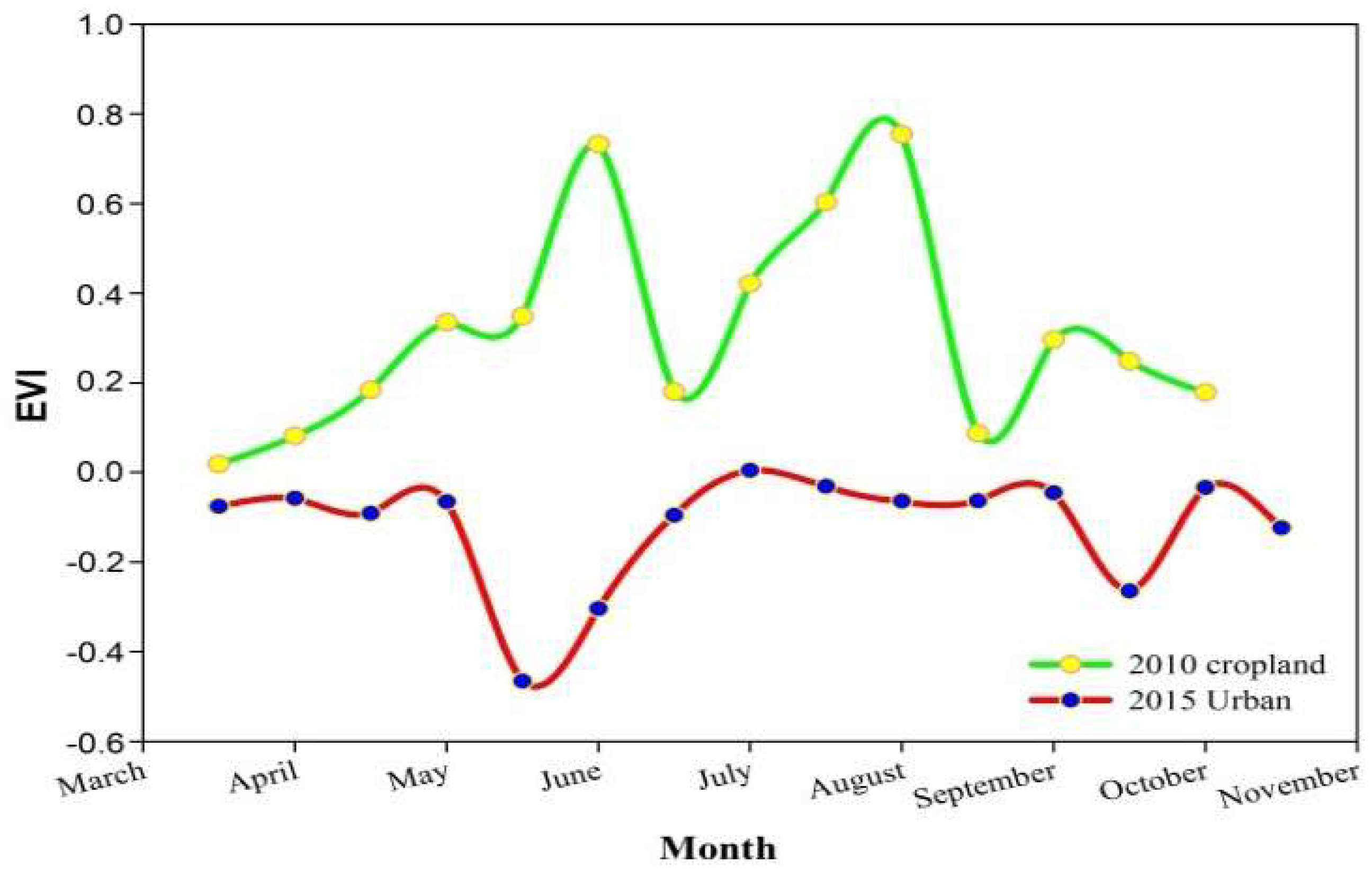
Generally, the phenological trajectory is characterized by baseline, amplitude, timing and shape. Across different years, the changing of land cover (e.g., natural or anthropogenic disturbances) causes the variation in amplitude, timing and shape of the phenological trajectories. For the pixel that changes from cropland to urban built-up, the trajectory of the EVI shows the biggest difference. Figure 4 shows the phenological trajectory of cropland based on the EVI time series derived from Landsat Enhanced Thematic Mapper Plus (ETM+) images in 2010 and of urban built-up based on EVI time series derived from Landsat OLI images in 2015. The examples illustrate that these changes could be detected by examining changes in amplitude, timing, and shape. Following this assumption, change detection is accomplished by measuring the similarity of the phenological trajectory of the same pixel at different years.

2.2.1. Phenological Trajectory Similarity Indicator

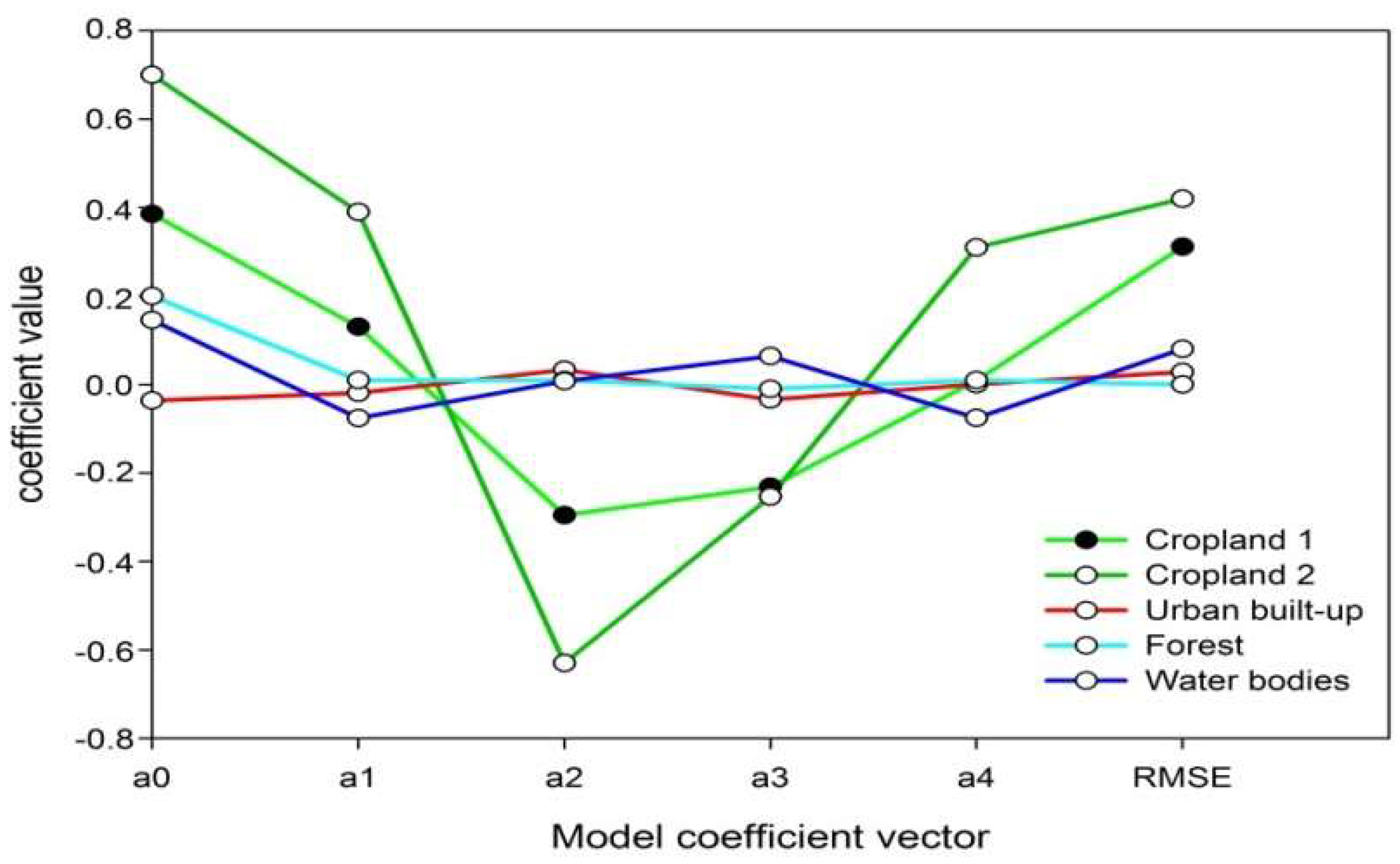
Once the phenological trajectory was generated, the coefficient vector $\mathit{C}\mathit{V}={\left({\mathrm{a}}_0, {\mathrm{a}}_1, {\mathrm{b}}_1, {\mathrm{a}}_2, {\mathrm{b}}_2, \mathrm{RMSE}\right)}^{\mathrm{T}}$ was extracted to fully excavate phenology information embedded in the temporal trajectory. The first five coefficients $({\mathrm{a}}_0, {\mathrm{a}}_1, {\mathrm{b}}_1, {\mathrm{a}}_2, \mathrm{and} {\mathrm{b}}_2)$ in the multi-harmonic model have definite physical significance associated with phenology. The zero-order coefficient ${\mathrm{a}}_0$ is the arithmetic mean of VI over the time series and represents the overall productivity of cropland. The first-term amplitude values ${\mathrm{a}}_1$ indicate the variability of productivity over the year. The first-term phase value ${\mathrm{b}}_1$ summarizes the timing of the growth stage. The amplitude ${\mathrm{a}}_2$ and phase ${\mathrm{b}}_2$ of second-order harmonic mainly describe the detailed phenological information of bimodal cropland activity (e.g., double or triple cropping a year) [48]. The root mean square error (RMSE) is used for assessing the fitness that indicates residual error. It is able to reflect the possibility of cropland change to some extent. For example, when cropland is changed to urban built-up, RMSE may get bigger since the harmonic model is not the most suitable for the urban area even though it can well fit the phenological trajectory of cropland. Figure 5 illustrates the model coefficients vector for four different kinds of land cover classes. It is clear that cropland shows quite different shapes in the plots of the six variables, especially ${\mathrm{a}}_2$ showing a lower value.

2.2.2. Change Detection Using Coefficient Vector Difference (CVD)

Directional cropland change, which results from natural and anthropogenic disturbances, could be detectable using harmonic analysis of the phenological trajectory by examining changes in CV. In the frequency domain, CV contains two components: ${\mathrm{a}}_1,{\mathrm{a}}_2$ represent the amplitude of trajectory and ${\mathrm{b}}_1,{\mathrm{b}}_2$ represent the phase of trajectory. On the one hand, amplitude scaling can cause intensity variations and occurs when the seasonal peak has been stretched or compressed in the y-axis. These intensity variations could be related to changes in vegetation vigor or coverage. Amplitude translation (i.e., when the time series has been shifted in the y-axis) is related to shifts in the background reflectance. On the other hand, phase effects (i.e., changing the width of the seasonal trajectory) could be related to changes in the length of the growing season due to an earlier or later onset of the growing season. The shape or values change of the VI time series (referring to the phenological trajectory here) can be the result of amplitude and phase effects. The shape of trajectory is important for deriving cropland phenological features, and values are also indispensable to describe the growth and change of the cropland. Therefore, both shape and value (i.e., amplitude and phase) differences are designed to quantitatively and qualitatively assessing changes of phenological trajectories of the same pixel at different years.

The similarity measurement is based on exploiting the differences of coefficient vector by considering amplitude and phase. Accordingly, it is assumed that the coefficient vectors of the pixel at year ${\mathrm{t}}_1$ and year ${\mathrm{t}}_2$ are given by $\mathit{C}{\mathit{V}}^{{\mathrm{t}}_1}$ and $\mathit{C}{\mathit{V}}^{{\mathrm{t}}_2}$, respectively, and the $\mathrm{CVD}$ is calculated as change magnitude as follows:

$$\begin{array}{ll}\mathrm{CVD}=& \left(\mathit{C}{\mathit{V}}^{{\mathrm{t}}_1},\mathit{C}{\mathit{V}}^{{\mathrm{t}}_2}\right)\\ & =\sqrt{{\displaystyle \sum }_{\mathrm{k}=0}^2{\left({\mathrm{a}}_{\mathrm{k}}^{{\mathrm{t}}_1}-{\mathrm{a}}_{\mathrm{k}}^{{\mathrm{t}}_2}\right)}^2}+\sqrt{{\displaystyle \sum }_{\mathrm{k}=1}^2{\left({\mathrm{b}}_{\mathrm{k}}^{{\mathrm{t}}_1}-{\mathrm{b}}_{\mathrm{k}}^{{\mathrm{t}}_2}\right)}^2}+\left|{\mathrm{RMSE}}^{{\mathrm{t}}_1}-{\mathrm{RMSE}}^{{\mathrm{t}}_2}\right|\end{array}$$

(2)

where k is the order number of the harmonic, the first term of the formula is the amplitude difference and the second term is the phase difference while the third term indicates the residual error of the harmonic model.

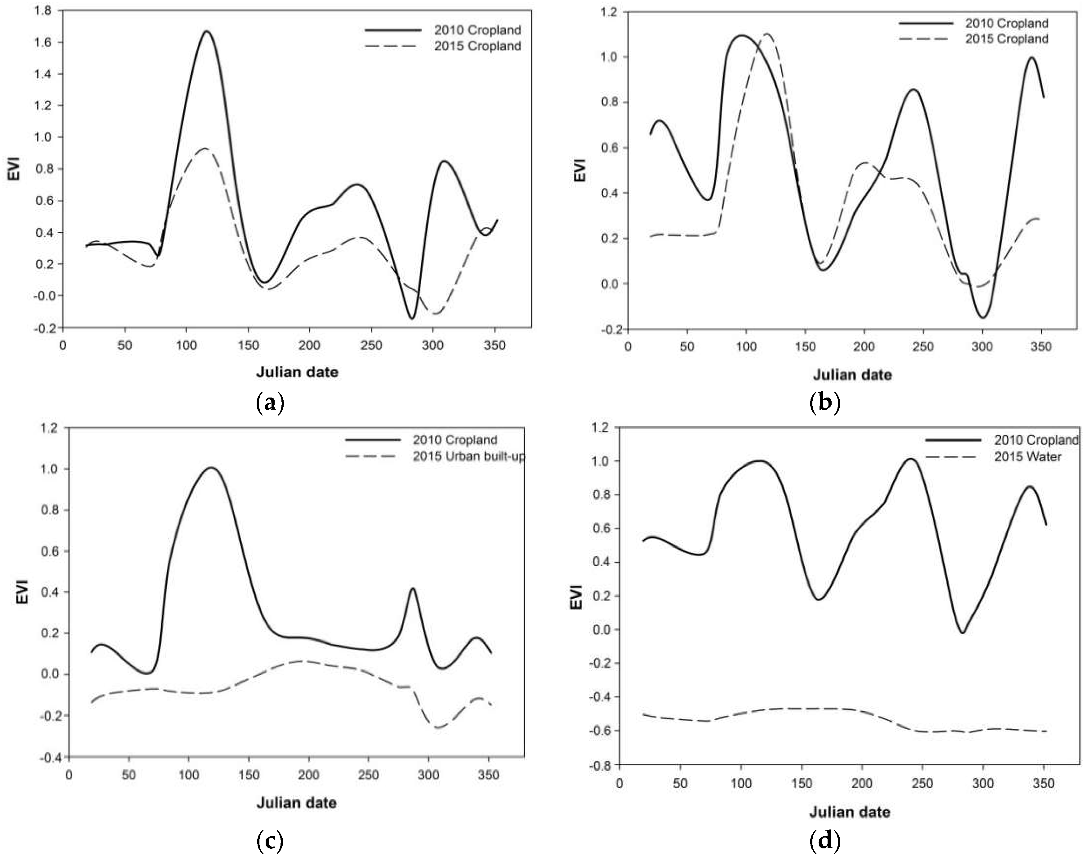
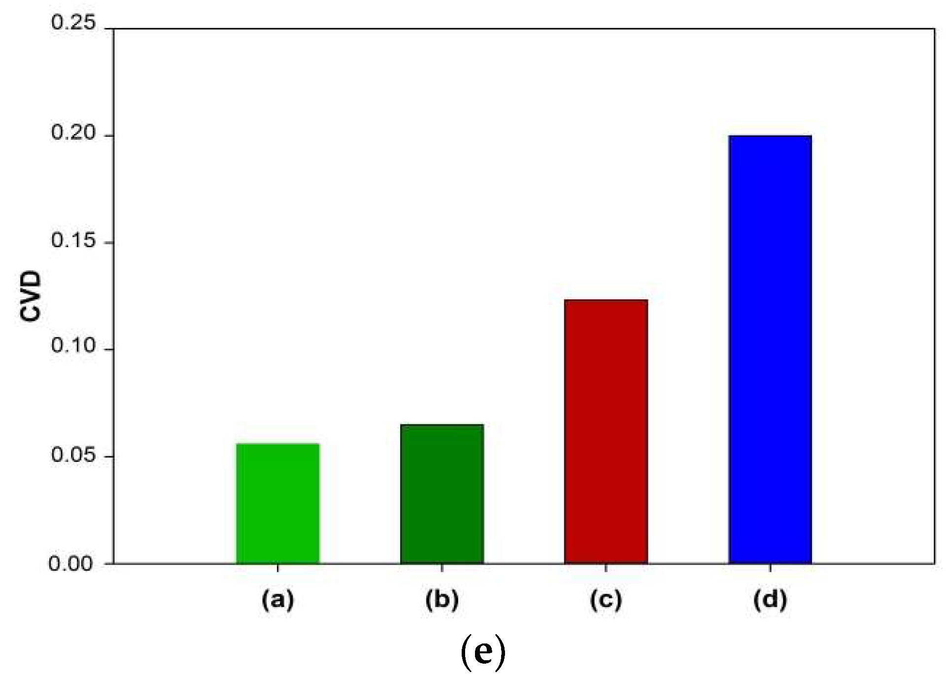
Figure 6 shows the phenological trajectory of cropland collected from the Landsat ETM+ time-series image in 2010 and Landsat OLI time-series image in 2015. Figure 6a shows amplitude effects occur due to different cropland types, which lead to the changing height peak of the EVI curve (i.e., the seasonal peak has been stretched or compressed in the y-axis). Figure 6b shows phase effects occur primarily due to a change of the rainy season, resulting in the time series being stretched or compressed in time, thus changing the width of the phenological trajectory. EVI curves of cropland at 2010, urban built-up and water at 2015 are compared in Figure 6c, Figure 6d, respectively. Based on the calculation of CVD, change magnitudes of the four pair EVI curves were computed. As shown in Figure 6e, the CVD between different cropland types shows a relatively small variance. Similarly, the CVD of cropland with different time location of the seasonal peak also has a small variance. In contrast, the CVD of change type from cropland to urban built-up and water is much larger. It means that the pseudo changes caused by differences of cropland type and influence of weather events (change of rainy season resulting in an earlier or later onset of the growing season) can be eliminated effectively based on CVD.

As for the magnitude of the change, a larger $\mathrm{CVD}$ indicates a greater possibility for changing. Given the magnitude image of change, a self-adaptive threshold algorithm called Expectation-Maximization (EM) can be used to detect the change/no-change areas. The EM algorithm applies an unsupervised assessment of prior probability density functions to automatically select the threshold to minimize the change-detection error probability. The pixels with greater magnitude than the threshold were labelled as changed pixels.

2.3. Change Type Discrimination Using Coefficient Ratio Vector (CRV)

It is more important to acquire the detailed “from-to” change information after detecting change areas [49]. However, for a pixel that has undergone a change from one class to another, the CV will definitely show a bigger difference. Different land cover change type has different change patterns of CV. Therefore, the coefficient ratio vector (CRV) was proposed here to determine change type both qualitatively and quantitatively. Firstly, the reference CRV of typical change types could be constructed based on the reference image. Then, the change type of the changed pixel could be determined based on the minimum distance between reference CRV and target CRV.

2.3.1. Reference CRV Construction

To determine the change types of changed pixels, the reference CRV is required for determining the change type of the changed pixel. In this study, we assume that the CRV differences between any two land cover types on t₁ are approximately equal to their CRV differences from t₁ to t₂. Therefore, the reference of a changed CRV was calculated on the reference image at t₁. First, a certain number of samples for each class was selected based on a known classification map on ${\mathrm{t}}_1$, and the CV of each class was derived from the harmonic model. Then, the mean value ${\overline{\mathit{C}\mathit{V}}}_i$ of each class could be calculated. Finally, the reference $\mathit{C}\mathit{R}{\mathit{V}}_{\mathrm{ij}}^{\mathrm{ref}}$ between any two kinds of land cover types i and j were calculated based on ${\overline{\mathit{C}\mathit{V}}}_{\mathrm{i}}$ and ${\overline{\mathit{C}\mathit{V}}}_{\mathrm{j}}$. The reference $\mathit{C}\mathit{R}{\mathit{V}}_{\mathrm{ij}}^{\mathrm{ref}}$ can be used for distance measuring, in order to discriminate change types from ${\mathrm{t}}_1 \mathrm{to} {\mathrm{t}}_2$.

$$\mathit{C}\mathit{R}{\mathit{V}}_{\mathrm{ij}}^{\mathrm{ref}}=\raisebox{1ex}{${\overline{\mathit{C}\mathit{V}}}_{\mathrm{i}}$}\!\left/ \!\raisebox{-1ex}{${\overline{\mathit{C}\mathit{V}}}_{\mathrm{j}}$}\right.={\left(\frac{{\overline{\mathrm{a}}}_{\mathrm{i},0}}{{\overline{\mathrm{a}}}_{\mathrm{j},0}},\frac{{\overline{\mathrm{a}}}_{\mathrm{i},1}}{{\overline{\mathrm{a}}}_{\mathrm{j},1}},\frac{{\overline{\mathrm{b}}}_{\mathrm{i},1}}{{\overline{\mathrm{b}}}_{\mathrm{j},1}},\frac{{\overline{\mathrm{a}}}_{\mathrm{i},2}}{{\overline{\mathrm{a}}}_{\mathrm{j},2}},\frac{{\overline{\mathrm{b}}}_{\mathrm{i},2}}{{\overline{\mathrm{b}}}_{\mathrm{j},2}},\frac{{\overline{\mathrm{RMSE}}}_{\mathrm{i}}}{{\overline{\mathrm{RMSE}}}_{\mathrm{j}}}\right)}^{\mathrm{T}}$$

(3)

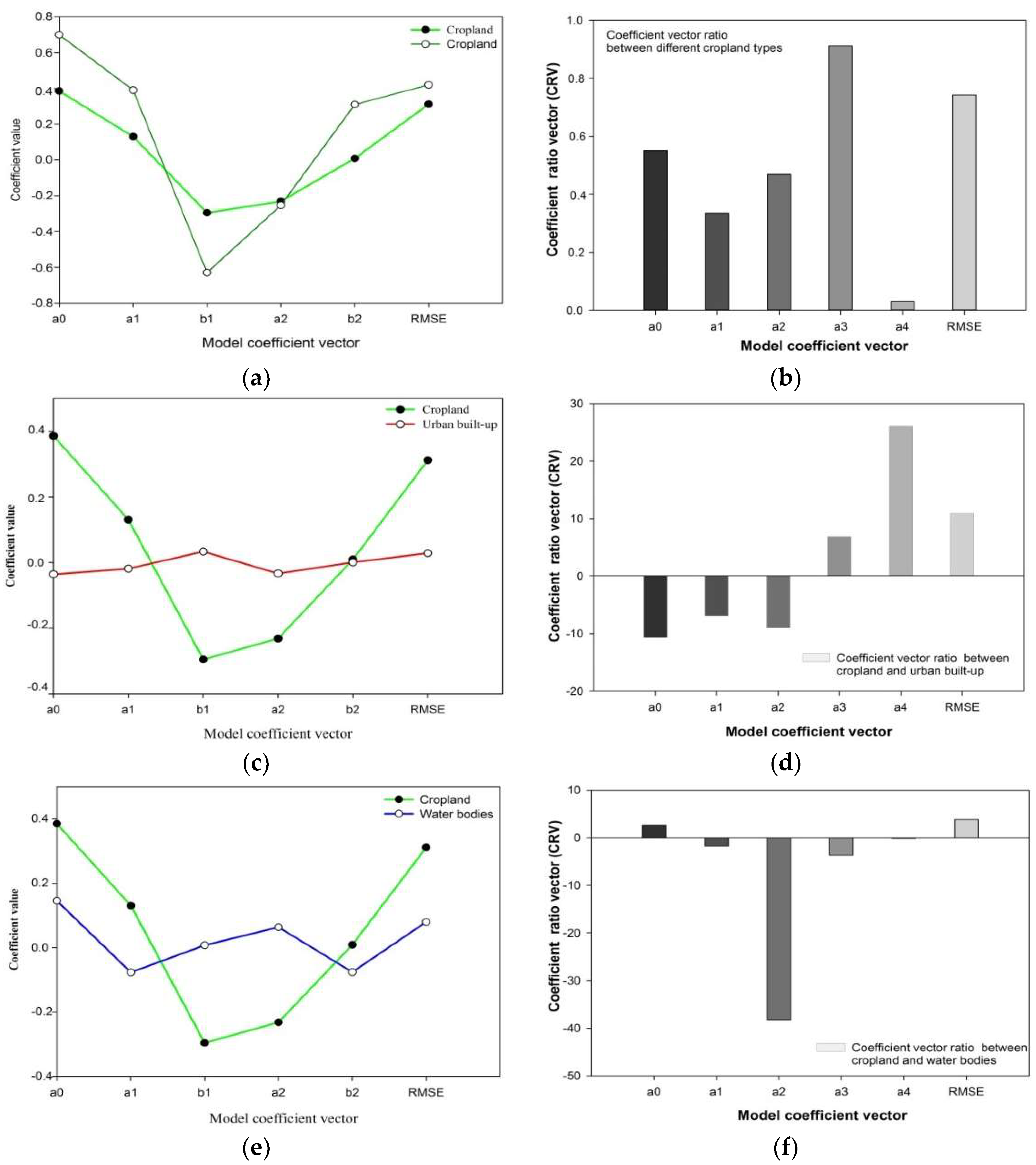
Based on the calculation of CRV, the model coefficient of examples in Figure 5 was used to acquire the coefficient ratio vector between different land cover types. Because different types of land cover have distinctive coefficient vectors, certain change types between two land cover types also have distinctive change patterns. Figure 7b shows the CRV between different cropland types, and Figure 7c,d shows the coefficient ratio vector of two change types from cropland to urban built-up and from cropland to water bodies respectively. As shown in Figure 7b, the CRV between different cropland types have the same signs (positive). When the changes occur from cropland to other land cover types (i.e., urban or water), the CRV signs are inconsistent and differ in different coefficients. This finding implies that different land cover change types have different CRV. Moreover, the value difference of CRV between the two land cover types shows much larger variance than between different cropland types. Therefore, the reference CRV should be constructed according to different signs (qualitatively) and values (quantitatively).

2.3.2. Change Type Discrimination by CRV Distance

After the change areas were identified, the changed pixel’s $\mathit{C}\mathit{R}{\mathit{V}}_{{\mathrm{t}}_1{\mathrm{t}}_2}^{\prime }$ from ${\mathrm{t}}_1 \mathrm{to} {\mathrm{t}}_2$ could also be computed:

$$\mathit{C}\mathit{R}{\mathit{V}}_{{\mathrm{t}}_1{\mathrm{t}}_2}^{\prime }={\left(\frac{{\mathrm{a}}_{{\mathrm{t}}_1,0}^{\prime }}{{\mathrm{a}}_{{\mathrm{t}}_2,0}^{\prime }},\frac{{\mathrm{a}}_{{\mathrm{t}}_1,1}^{\prime }}{{\mathrm{a}}_{{\mathrm{t}}_2,1}^{\prime }},\frac{{\mathrm{b}}_{{\mathrm{t}}_1,1}^{\prime }}{{\mathrm{b}}_{{\mathrm{t}}_2,1}^{\prime }},\frac{{\mathrm{a}}_{{\mathrm{t}}_1,2}^{\prime }}{{\mathrm{a}}_{{\mathrm{t}}_2,2}^{\prime }},\frac{{\mathrm{b}}_{{\mathrm{t}}_1,2}^{\prime }}{{\mathrm{b}}_{{\mathrm{t}}_2,2}^{\prime }},\frac{{\mathrm{RMSE}}_{{\mathrm{t}}_1}^{\prime }}{{\mathrm{RMSE}}_{{\mathrm{t}}_2}^{\prime }}\right)}^{\mathrm{T}}$$

(4)

Suppose the pixel belongs to cropland at ${\mathrm{t}}_1$, the corresponding reference CRV from cropland to others can be selected. Then, the change type is be determined based on the minimum distance between the reference $\mathit{C}\mathit{R}{\mathit{V}}_{\mathrm{ij}}^{\mathrm{ref}}$ and the $\mathit{C}\mathit{R}{\mathit{V}}_{{\mathrm{t}}_1{\mathrm{t}}_2}^{\prime }$ of the changed pixel.

$$\mathrm{D}(\mathit{C}\mathit{V}{\mathit{R}}_{{\mathrm{t}}_1{\mathrm{t}}_2}^{\prime },\mathit{C}\mathit{V}{\mathit{R}}_{\mathrm{ij}}^{\mathrm{ref}})=\min \left\{\sum \left|\mathit{C}\mathit{V}{\mathit{R}}_{{\mathrm{t}}_1{\mathrm{t}}_2}^{\prime }-\mathit{C}\mathit{V}{\mathit{R}}_{12}^{\mathrm{ref}}\right|,\sum \left|\mathit{C}\mathit{V}{\mathit{R}}_{{\mathrm{t}}_1{\mathrm{t}}_2}^{\prime }-\mathit{C}\mathit{V}{\mathit{R}}_{13}^{\mathrm{ref}}\right|,\cdots \sum \left|\mathit{C}\mathit{V}{\mathit{R}}_{{\mathrm{t}}_1{\mathrm{t}}_2}^{\prime }-\mathit{C}\mathit{V}{\mathit{R}}_{\mathrm{ij}}^{\mathrm{ref}}\right|\right\}$$

(5)

A smaller D value indicates a higher similarity, and the change type of the changed pixel is then assigned to the class with the minimum $\mathrm{D}\left(\mathit{C}\mathit{V}{\mathit{R}}_{{\mathrm{t}}_1{\mathrm{t}}_2}^{\prime },\mathit{C}\mathit{V}{\mathit{R}}_{\mathrm{ij}}^{\mathrm{ref}}\right)$.

3. Study Area and Data

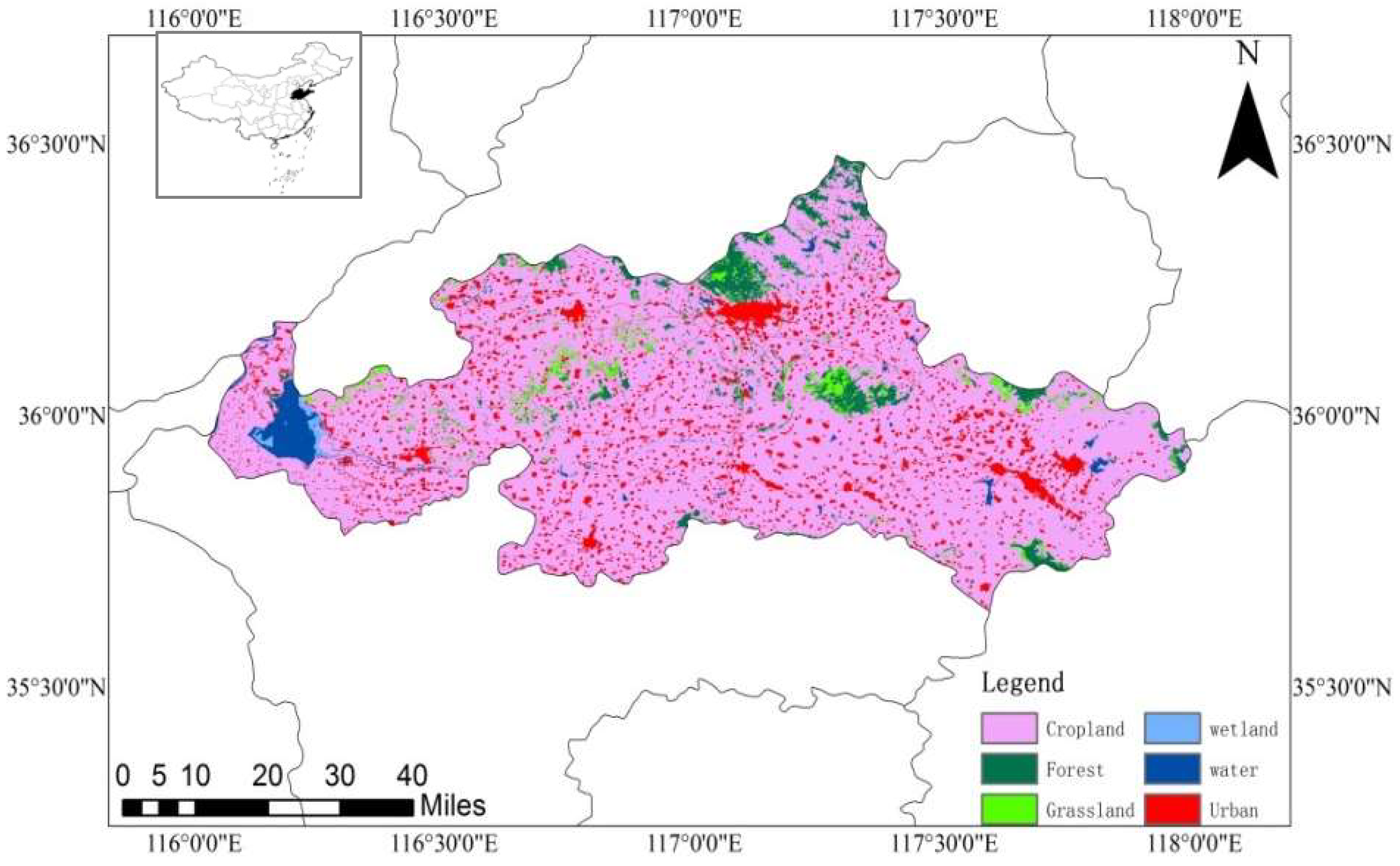
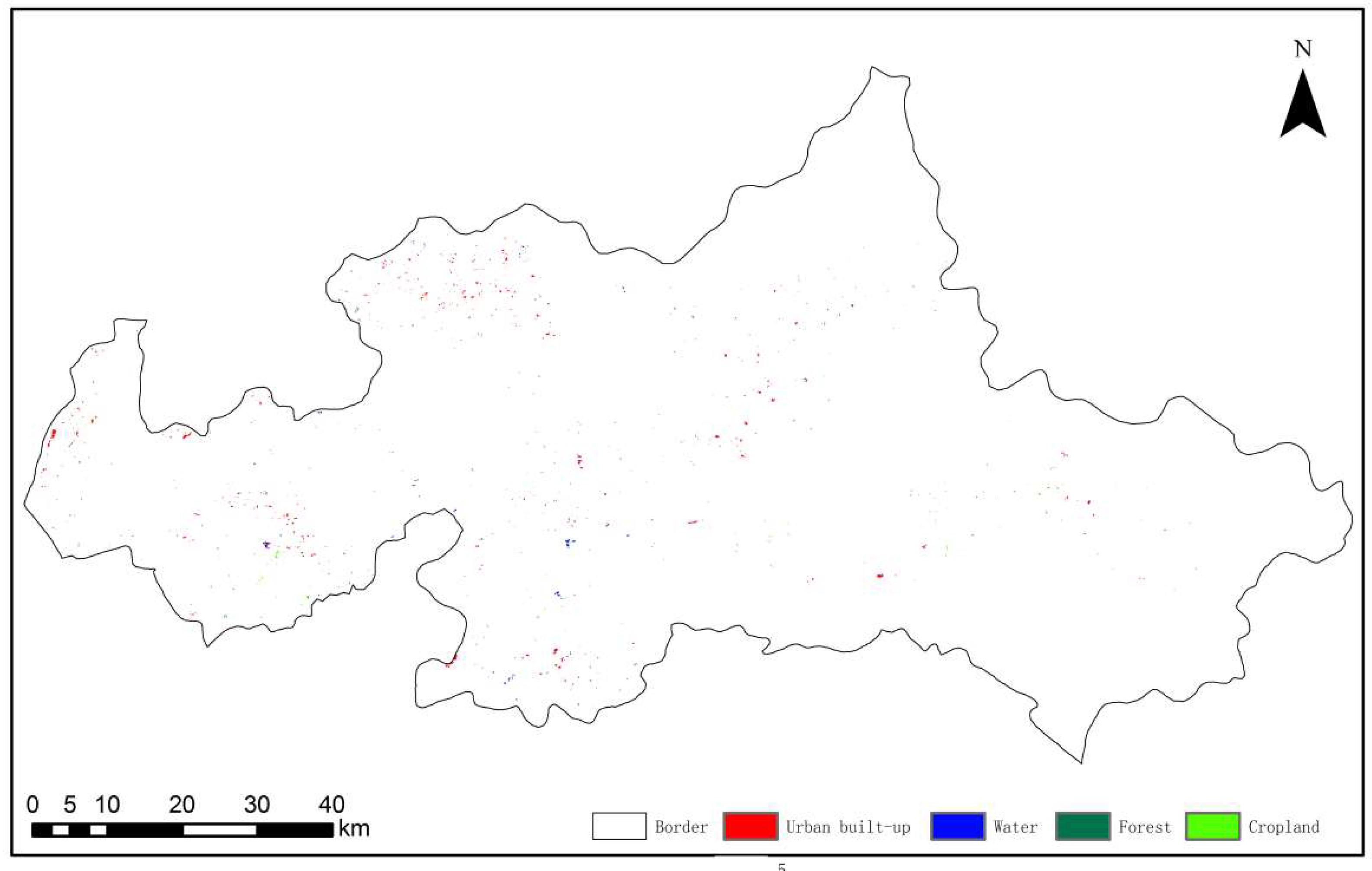
Our study area belongs to the North China Plain located in central Shandong Province, China, bound by 35°39′ to 36°12′N and 115°55′ to 116°23′E (Figure 8). Mean annual temperature is 12.9 °C and mean annual precipitation is 687 mm 32% falling in July. There are some zones of mountainous areas, but the region is dominated by agriculture. The main land cover types of the area are cropland, water, urban built-up, forest, and barren. There are two types of cropping systems in our study area. The dual cropping system is composed of winter wheat and summer corn, and the single cropping system is mostly peanuts. Over the past few decades, rapid industrialization and urbanization have greatly changed the agricultural land pattern in this study area.

We used a series of Landsat sensors Thematic Mapper (TM), Enhanced Thematic Mapper Plus (ETM+), and Operational Land Imager (OLI) image for Path 122, Row 35 for the years 2009, 2010, 2015, 2016 (

Table 1. Description of Landsat images (including Thematic Mapper (TM), Enhanced Thematic Mapper Plus (ETM+), and Operational Land Imager (OLI) image) used in the analysis.

Number	Date	Sensor	Number	Date	Type
1	10 January 2009	ETM	1	19 January 2015	OLI
2	10 March 2010	TM	2	4 February 2015	OLI
3	3 April 2010	ETM	3	24 March 2015	OLI
4	16 April 2009	ETM	4	25 April 2015	OLI
5	27 April 2010	TM	5	13 May 2016	OLI
6	3 June 2009	ETM	6	12 June 2015	OLI
7	22 June 2010	ETM	7	14 July 2015	OLI
8	17 August 2010	TM	8	1 August 2016	OLI
9	30 August 2009	TM	9	2 September 2016	OLI
10	10 September 2010	ETM	10	2 October 2015	OLI
11	17 October 2009	TM	11	3 November 2015	OLI
			12	21 December 2015	OLI

) assuming no cropland change had occurred within neighboring two years. Two years (2009 and 2010) of Landsat TM and ETM+ images (11 images) were selected as time-series data at t₁ year, and another two years (2015 and 2016) of Landsat OLI images (12 images) were used as time-series data at t₂ year.

Image preprocessing is critical to the change detection, facilitating comparison of time series images. Image preprocessing mainly includes geo-referencing, atmospheric correction, and cloud and cloud shadows detection. First, to convert all raw imagery from the DN to surface reflectance values, we used the Landsat Ecosystem Disturbance Adaptive Processing System (LEDAPS) developed by the United States Geological Survey (USGS) to perform automatic atmospheric correction. The LEDAPS algorithm is a highly standardized preprocessing tool that ensures the compressibility of reflectance values from different sensors. The algorithm also requires some ancillary data such as water vapor and ozone concentration. LEDAPS source code and ancillary data can be downloaded from USGS. Second, cloud, cloud shadows and snow were detected using the object-based Fmask algorithm. We used Bands 1, 2, 3, 4, 5, 7 and Band 6 Brightness Temperature (BT) as input data. Fmask ulitizes rules based on cloud physical properties and an object matching approach to extract cloud, cloud shadows, and snow. Finally, relative radiometric normalization was performed using multivariate alteration detection and calibration (MADCAL) algorithms [48]. After the cloud and cloud shadow masking steps were completed for all images, pixels labelled as cloud or cloud shadows were not used in the proposed method. One strategy to complete the integrity of the time-series was the linear-interpolation technology: the masked pixels were given a value according to the trajectory of the clear observations. Specifically, for each masked pixel in a particular day i, the temporally nearest clear observations acquired before (b) and after (a) day i were used to drive its value as follows:

$$R_i=R_b+\left(i-b\right)\times \frac{R_a-R_b}{a-b}$$

(6)

where a and b are before and after day i, respectively; and $R_a,R_b,\mathrm{and}{R}_i$ are the reflectance values on a, b, and i, respectively.

There are several non-cropland types in our study area, such as water bodies, barren land, and artificial surfaces. To avoid confusion between cropland and other land cover types, we extracted a cropland mask and only assessed these pixels for change. We detected cropland change from t₁ year to t₂ year, and cropland mask was made only for images from the t₁ year. That is to say, the changes we detected are from cropland to other types. In our experiment, the Landsat images from 2010 were selected as time-series data at t₁ year. Therefore, the cropland mask of images at the t₁ year was produced using Globeland30 2010. Meanwhile high spatial resolution images from Google Earth were used to help manual interpretation. If there was confusion in comparing the two Landsat images, high spatial resolution images before and after 2010 (can be a few years apart) from Google Earth were used to help determine what was happening at the specific locations. The land cover of each reference point was checked against the Google Earth image with sub-meters spatial resolution.

4. Results

4.1. Change Areas Detection

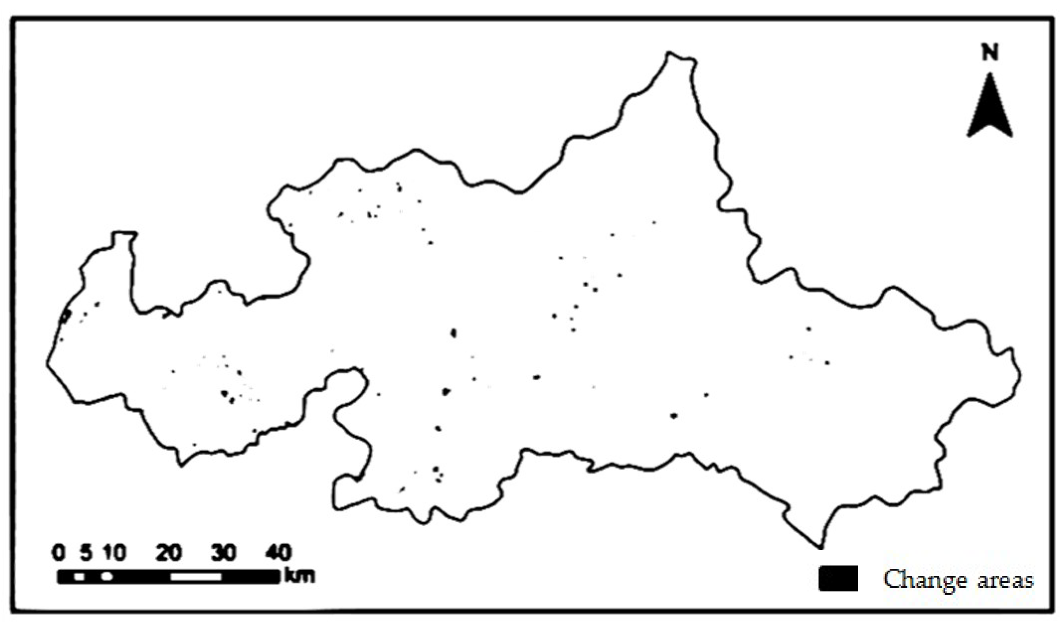
The proposed change detection method was used to estimate the change magnitude of the phenological trajectory between the two years (t₁ and t₂). Generally, pixels having relatively large magnitudes were labelled as changed areas, and those pixels with smaller magnitudes were classified as unchanged areas. The EM algorithm was used to determine the threshold for change detection. These images of change area were formatted as binary images and used as mask files for further change type discrimination (Figure 9).

The results show signs of cropland change pattern, as indicated by the reduction in cropland area (Figure 9). However, most of the reduction in cropland can be found geographically in the northwest and southwest parts. These changes in the landscape of Tai’an are mainly the outcome of the continuous urban sprawl of the urban district region over the past five years (2010–2015). Change detection results only including change and no-change classes showed high performance for detection accuracy, with an overall accuracy (OA) value of 98.58% and kappa coefficient of 0.82 (

Table 2. Confusion matrix of change/no-change detection results.

Classified Changed (Pixels)	Reference Changed (Pixels)
	No-Change	Change	Sum	Commission Error
Nochange	48,130	715	48,845	1.46
Change	2	1672	1674	0.12
Sum	48,132	2387	50,519
Omission error	0.00	29.95
OA(%) = 98.58%, Kappa coefficient = 0.82

).

To evaluate the improvement and effectiveness of our method, the change areas detection results of the three other methods, CCDC, CVA, and PCC, were calculated for comparison and analysis. In the CCDC method, two years (2009 and 2010) of time-series images (11 images) were used as input data to describe the trend, and predicted images value at 2015. Then, the differences between model predicted and observed value were used to detect the change areas. CVA and PCC were separately conducted based on several Landsat images acquired on 3 April 2010 and 2 October 2015. To visually inspect areas of change or no-change in detail, four subset areas of the change detection results were selected (Figure 10 and Figure 11).

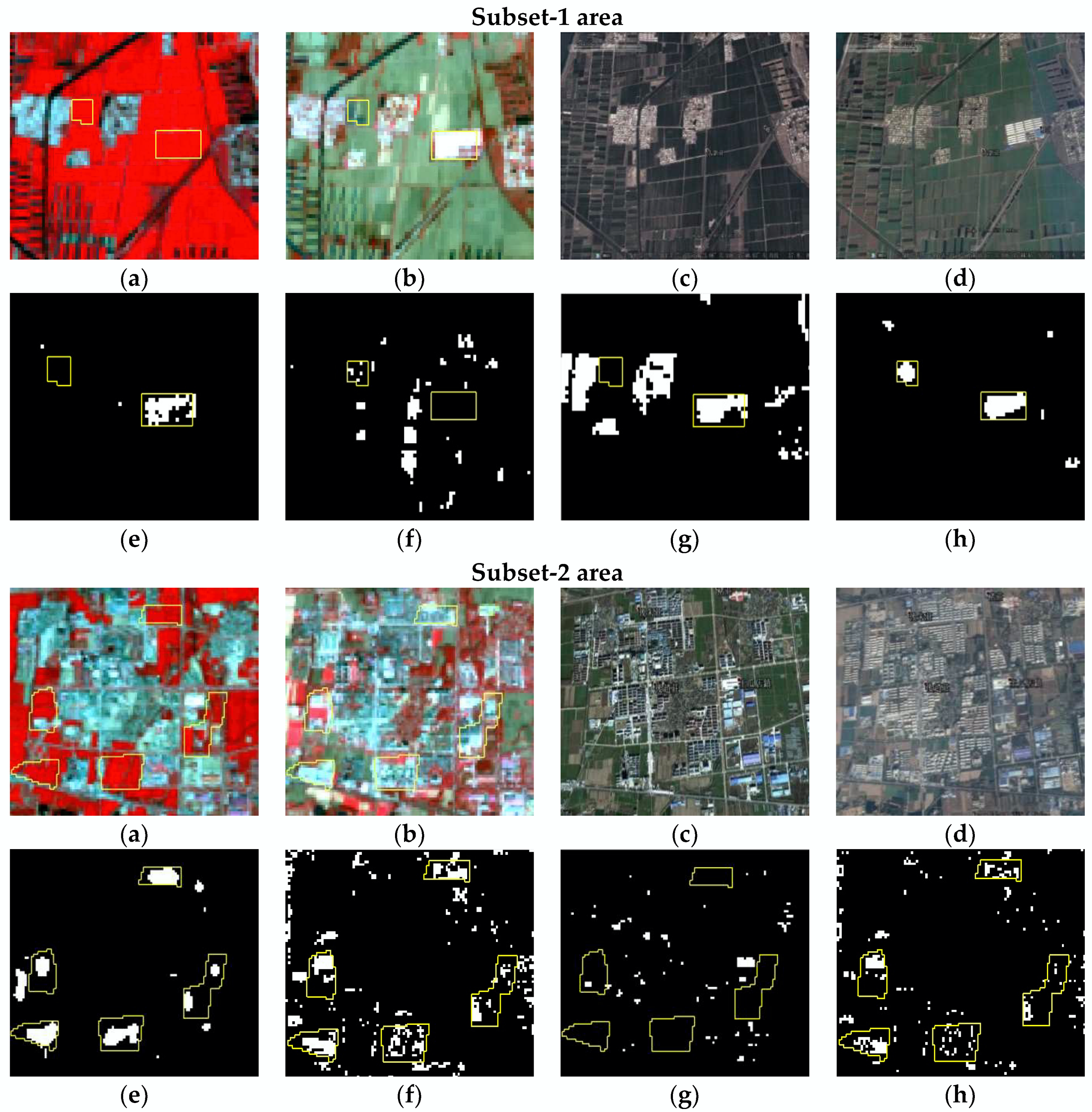
Figure 10 shows cropland related changes from cropland to urban built-up are the primary changes that occurred between the two time periods for the subset-1 and subset-2 area. The area inside the yellow polygon changed from 2010 to 2015 according to Google earth image with higher resolution. In subset-1 area, the results show that changes associated with urban development are correctly identified using the proposed method. Although the obvious changes were very well detected in CCDC, the subtle changes were not well detected in this image. By contrast, CVA and PCC detected many pseudo changes instead of true changes. This might be because the change magnitude of cropland pseudo changes is greater than that of real change from cropland to urban built-up. Similarly, for subset-2 area, although the CCDC also correctly identified real changes, it also produced a lot of pseudo changes or pepper and salt noises. The achieved results indicate superiority of the proposed method to other methods in detecting real changes.

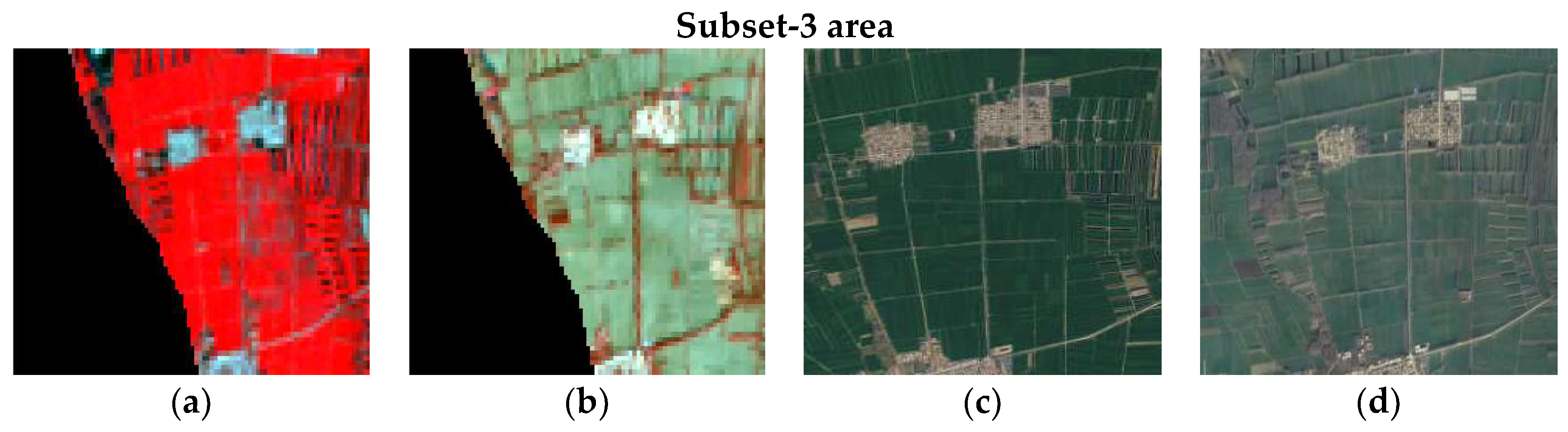
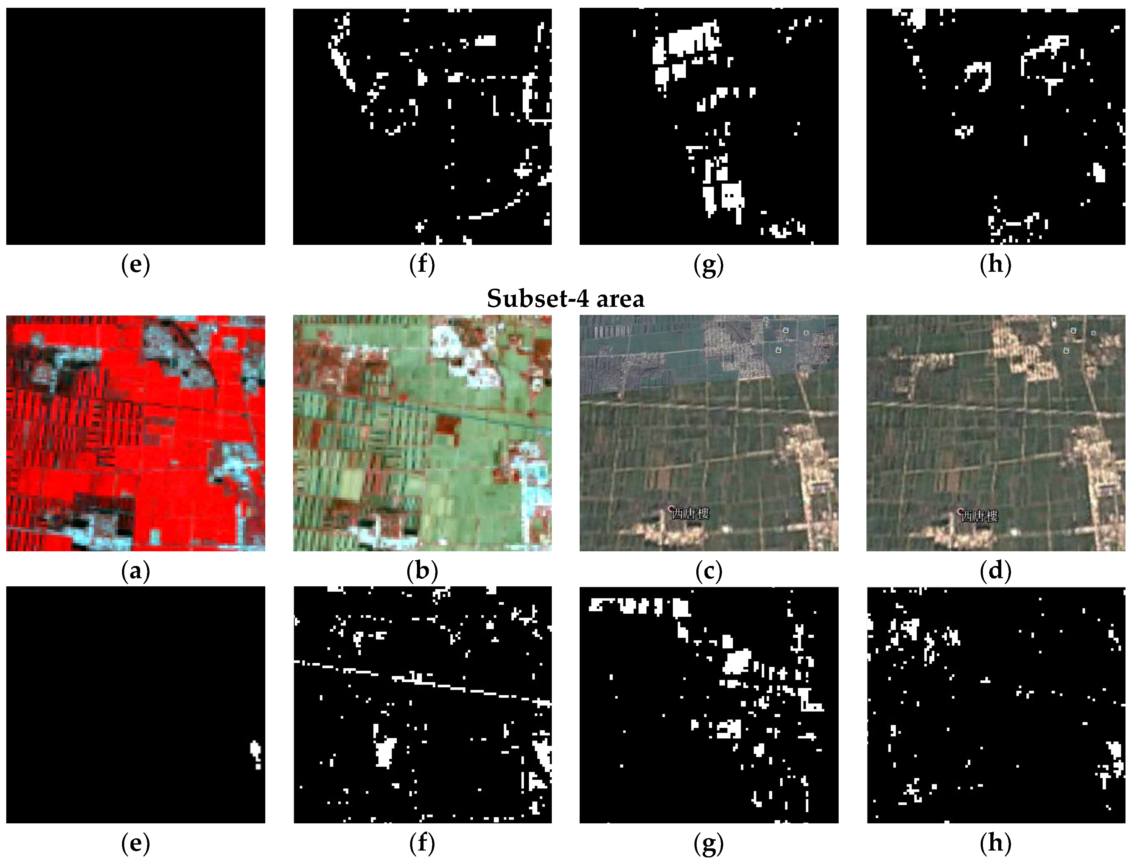
As shown in Figure 11 (the subset-3 and subset-4 area, respectively), the two subset areas remained unchanged from 2010 to 2015 according to the Google earth image. The result shows that pseudo changes are not produced in the proposed method. It is clear that our method outperforms the other three methods in the capacity of elimination of pseudo change caused by seasonal difference. For cropland that likely has a large spectral change but not a real cover change, our method significantly eliminated these changes by combining the difference of the phenological trajectories. However, CCDC, CVA, and PCC captured these apparent spurious changes because of a larger change magnitude resulting from crop rotation, irrigation, and seasonality.

The accuracy assessment with the same test samples is shown in

Table 3. Accuracies of the four change detection methods.

	The Proposed Method	Continuous Change Detection and Classification (CCDC)	Change Vector Analysis (CVA)	Post-Classification Comparison (PCC)
Thresholds	1.5	1.0	82.57	78.14
OA (%)	98.58	95.23	93.96	93.42
Kappa coefficient	0.82	0.79	0.66	0.78

. It is clear that the proposed method acquired the highest accuracy with an overall accuracy of 98.58% and a kappa coefficient of 0.82. The CCDC has a higher accuracy than the CVA and PCC method with the overall accuracy of 95.23% and a kappa coefficient of 0.79. By contrast, the CVA and PCC method with the lower accuracy provided relatively less reliable results for cropland change detection.

4.2. Change Type Discrimination

Once the change areas were identified, the change type could be discriminated based on CRV distance. Globeland30 2010 was used as a baseline for acquiring training datasets from unchanged pixels. The classification of the change type was performed by first calculating the difference between the CRV of the change pixel and each reference pixel using Equation (5). The change type of pixel was then assigned to the class with the minimum D.

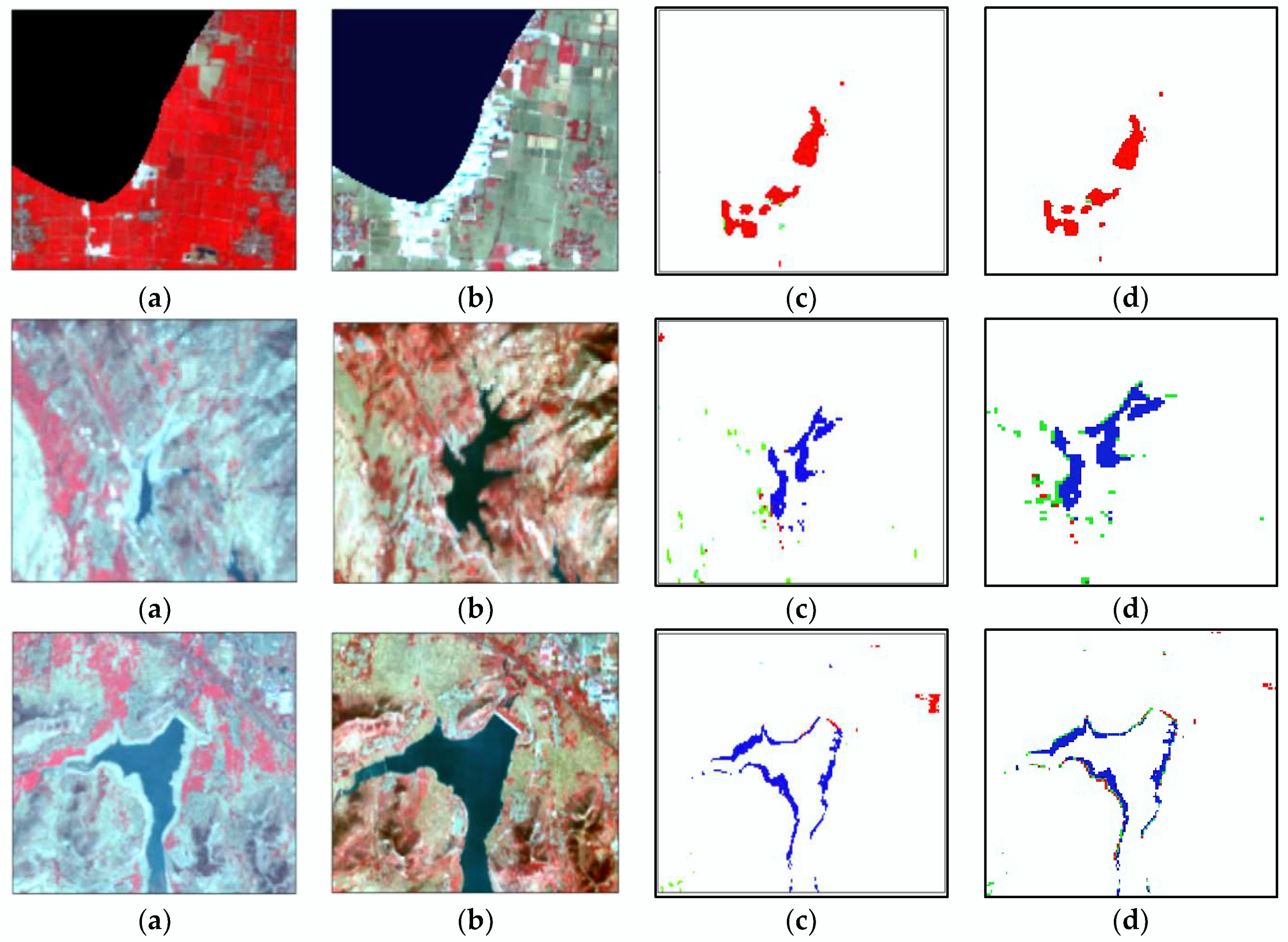
The change type discrimination results by using the CRV distance are presented on Figure 12. For comparison, the CCDC classification method was used for the same training data for image classification. The CCDC uses the model coefficients as the inputs for land cover classification. As an example, the results of change type discrimination by using both the CRV distance and CCDC are presented on Figure 13. As shown in the subset-1 area, the apparent changes are from urban developments that typically consume surrounding agricultural land. The region experiences apparent cropland changes caused by both urban developments in suburban areas. Most landscape change was related to urban development to meet the growing population in the region. Other obvious changes are from cropland to water bodies (subset-2 and subset-3 areas). The changed areas may be seasonal rivers. Cropland areas are actually the lake surface area that was dried before 2010. The expanded water surface area may be due to an increase in rainfall.

To evaluate the ability to discriminate change type and assess the accuracy of the proposed method, we computed a confusion matrix and derived the overall accuracy and overall kappa index.

Table 4. Confusion matrix of classification results from the proposed method.

Classified Data (%)	Reference Data (%)				User’s Accuracy
	Cropland	Forest	Urban	Water
Cropland	96.93	3.57	10.22	0.00	35.95
Forest	0.54	90.19	1.66	0.08	99.70
Urban	2.54	5.23	87.95	1.27	71.96
Water	0	1.01	0.17	98.65	47.14
Producer’s accuracy	96.93	90.19	87.95	98.65
OA(%) = 90.13%, Kappa coefficient = 0.71

and

Table 5. Confusion matrix of classification results from the CCDC method.

Classified Data (%)	Reference Data (%)				User’s Accuracy
	Cropland	Forest	Urban	Water
Cropland	74.82	1.83	2.68	0.30	97.21
Forest	17.74	96.85	5.49	0.21	40.02
Urban	7.44	1.33	91.65	4.80	74.02
Water	0.00	0.00	0.18	94.70	99.95
Producer’s accuracy	74.82	96.85	91.65	74.82
OA(%) = 88.55%, Kappa coefficient = 0.82

show the confusion matrixes for change areas classifications by CRV difference and CCDC, respectively. The classification accuracy and kappa coefficient are 90.13%, and 0.71 by the CRV distance, and 88.55% and 0.82 by the CCDC method. This indicates that the CRV distance exceeds the CCDC method in overall accuracy.

5. Discussion

The experimental results (Table 3, Figure 10 and Figure 11) indicate that the proposed method provides the capacity to detect real changes and estimate pseudo changes caused by season differences. The possible reasons are as follows. First, the proposed method effectively weakens the influence of seasonal differences and noise because data are collected throughout the growing season. Although the CCDC also makes full use of time-series images, the simple sinusoidal model used for CCDC fails to fully describe the complex features of cropland. Second the multi-harmonic model was used for describing the phenological trajectory, which widens the gap between cropland and other land cover types to some extent. Finally, the proposed method is mainly based on the similarity between temporal trajectories instead of direct comparison between the two points. Thus, the final change detection result is equivalent to the comprehensive results from different season differences.

In addition, the proposed method discriminated change type by CRV distance instead of only model coefficients as with the CCDC. The classification accuracy of the proposed method is better than that of the CCDC (Figure 13, Table 4 and Table 5). One possible explanation is that the large spectral variance within the cropland class makes accurate classification difficult. In the CCDC, several variables from the simple harmonic model are used as inputs for classification. However, cropland possesses complicated spectral features and unique phenological characteristics. The simple sinusoidal model including several variables is fully unable to discriminate cropland from other land cover type. The same land cover type is still more likely to have different model variables. The CRV including six coefficients is capable of maximizing the difference between cropland and other land cover types. Therefore, the result indicates that the CRV distance is a more effective method for change type discrimination compared with the CCDC method. However, we should note that since the result of the proposed method depends on the study area and data, it is necessary that further analysis is conducted to validate the extent to which the method holds true in other regions or with different resolutions.

This work indeed provided a novel method to detect changes but could be further improved and enhanced. However, further research needs to be considered as follows.

(1)

Our method focused on the intra-annual variations within the EVI time series. Further research is necessary to study inter-annual variations related to plant phenology. However, the multi-harmonic model including first and second order harmonics may not be sufficient to fully capture its inter-annual trend. An advanced time-series model should be constructed to capture both intra-annual and inter-annual trend.

(2)

Future algorithm improvements may include the capacity to eliminate phenological changes caused by change of cropland types or transformation of the farming system. In this study we focused on the shape similarity of the phenological trajectory while neglecting the phenological value difference. The main phenological parameters changes should be also considered as part of the change magnitude. This illustrates that further work is needed to extract the key phenological parameters.

(3)

Although our method acquired higher accuracy on change type discrimination, reference CRV only includes three change types (“from cropland to” changes). To identify the decrease and increase of cropland, a knowledge base of reference CRV including all change types is necessary.

6. Conclusions

One of the major challenges in cropland change detection is how to detect true changes while reducing false changes caused by seasonal differences and other interference factors. The change detection method based on time series images effectively weakens the influence of seasonal differences and noise because data are collected throughout the growing seasons. In this research, a new change detection method based on phenological trajectory similarity was designed and implemented to capture cropland changes. The core concept of the proposed method is detecting true cropland changes based on the similarity between temporal trajectories instead of the direct comparison between the two images. Due to the complex spectral-temporal characteristic of cropland, the phenological trajectory was constructed using a multi-harmonic model for capturing intra-annual variations. Then, to make full use of the spectral–temporal–phenological information, the CVD was calculated to measure similarity and identify change/no-changes areas. Moreover, it will be more important if we know the detail “from cropland to” change information. Instead of the traditional classification method based on original images, we used the coefficient ratio vectors (CRV) as the inputs for change type discrimination. The proposed method integrates spectral information, phenological information, and temporal characteristics to acquire a maximum possible change map with the goal of minimizing pseudo changes caused by seasonal differences. Our method was applied to the EVI time series derived from Landsat images for a cropland study area in eastern China. Results showed that the proposed method has the highest accuracy of change detection (98.58%) and a lower commission error than the other methods. The proposed method can avoid the strict requirement of CVA or PCC for image acquisition in that two images acquired in different years should be from the same seasonal period. In addition, this study presents a change type discrimination method based on the distance between the CRV of the changed pixel and of the reference change type. The result of the change type classification (OA of 90.13% and kappa index of 0.71) confirmed the efficiency of the method in discriminating the main change types.

References

- Deng, Y.; Liu, S.; Lu, M.; Song, C. Causes of cultivated land loss in mountainous areas protected for water sources case study of Miyun county in Beijing. J. Food Agric. Environ. 2012, 10, 685–690. [Google Scholar]
- Disperati, L.; Virdis, S.G.P. Assessment of land-use and land-cover changes from 1965 to 2014 in Tam Giang-Cau Hai Lagoon, central Vietnam. Appl. Geogr. 2015, 58, 48–64. [Google Scholar] [CrossRef]
- Tottrup, C.; Rasmussen, M.S. Mapping long-term changes in savannah crop productivity in senegal through trend analysis of time series of remote sensing data. Agric. Ecosyst. Environ. 2004, 103, 545–560. [Google Scholar] [CrossRef]
- Wardlow, B.D.; Egbert, S.L. Large-area crop mapping using time-series modis 250 m NDVI data: An assessment for the U.S. Central Great Plains. Remote Sens. Environ. 2008, 112, 1096–1116. [Google Scholar] [CrossRef]
- Schmidt, M.; Pringle, M.; Devadas, R.; Denham, R.; Tindall, D. A framework for large-area mapping of past and present cropping activity using seasonal landsat images and time series metrics. Remote Sens. 2016, 8, 312. [Google Scholar] [CrossRef]
- Gao, F.; Anderson, M.C.; Zhang, X.; Yang, Z.; Alfieri, J.G.; Kustas, W.P.; Mueller, R.; Johnson, D.M.; Prueger, J.H. Toward mapping crop progress at field scales through fusion of landsat and modis imagery. Remote Sens. Environ. 2017, 188, 9–25. [Google Scholar] [CrossRef]
- Dempewolf, J.; Adusei, B.; Becker-Reshef, I.; Hansen, M.; Potapov, P.; Khan, A.; Barker, B. Wheat yield forecasting for Punjab province from vegetation index time series and historic crop statistics. Remote Sens. 2014, 6, 9653–9675. [Google Scholar] [CrossRef]
- Hilson, G. An overview of land use conflicts in mining communities. Land Use Policy 2002, 19, 65–73. [Google Scholar] [CrossRef]
- Manjunath, K.R.; Panigrahy, S.; Kumari, K.; Adhya, T.K.; Parihar, J.S. Spatiotemporal modelling of methane flux from the rice fields of India using remote sensing and GIS. Int. J. Remote Sens. 2006, 27, 4701–4707. [Google Scholar] [CrossRef]
- Wulder, M.A.; White, J.C.; Goward, S.N.; Masek, J.G.; Irons, J.R.; Herold, M.; Cohen, W.B.; Loveland, T.R.; Woodcock, C.E. Landsat continuity: Issues and opportunities for land cover monitoring. Remote Sens. Environ. 2008, 112, 955–969. [Google Scholar] [CrossRef]
- Belward, A.S.; Skøien, J.O. Who launched what, when and why; trends in global land cover observation capacity from civilian earth observation satellites. ISPRS J. Photogramm. Remote Sens. 2015, 103, 115–128. [Google Scholar] [CrossRef]
- Radke, R.J.; Andra, S.; Al-Kofahi, O.; Roysam, B. Image change detection algorithms: A systematic survey. IEEE Trans. Image Process. 2005, 14, 294–307. [Google Scholar] [CrossRef] [PubMed]
- Hussain, M.; Chen, D.; Cheng, A.; Wei, H.; Stanley, D. Change detection from remotely sensed images: From pixel-based to object-based approaches. ISPRS J. Photogramm. Remote Sens. 2013, 80, 91–106. [Google Scholar] [CrossRef]
- Tewkesbury, A.P.; Comber, A.J.; Tate, N.J.; Lamb, A.; Fisher, P.F. A critical synthesis of remotely sensed optical image change detection techniques. Remote Sens. Environ. 2015, 160, 1–14. [Google Scholar] [CrossRef] [Green Version]
- Bruzzone, L.; Cossu, R.; Vernazza, G. Detection of land-cover transitions by combining multidate classifiers. Pattern Recognit. Lett. 2004, 25, 1491–1500. [Google Scholar] [CrossRef]
- Lu, D.; Mausel, P.; Brondízio, E.; Moran, E. Change detection techniques. Int. J. Remote Sens. 2004, 25, 2365–2401. [Google Scholar] [CrossRef]
- Chen, J.; Chen, X.; Cui, X.; Chen, J. Change vector analysis in posterior probability space: A new method for land cover change detection. IEEE Geosci. Remote Sens. Lett. 2011, 8, 317–321. [Google Scholar] [CrossRef]
- Johnson, R.D.; Kasischke, E.S. Change vector analysis: A technique for the multispectral monitoring of land cover and condition. Int. J. Remote Sens. 1998, 19, 411–426. [Google Scholar] [CrossRef]
- Lu, M.; Chen, J.; Tang, H.; Rao, Y.; Yang, P.; Wu, W. Land cover change detection by integrating object-based data blending model of landsat and modis. Remote Sens. Environ. 2016, 184, 374–386. [Google Scholar] [CrossRef]
- Bruzzone, L.; Prieto, D.F. Automatic analysis of the difference image for unsupervised change detection. IEEE Trans. Geosci. Remote Sens. 2000, 38, 1171–1182. [Google Scholar] [CrossRef]
- Gómez, C.; White, J.C.; Wulder, M.A. Optical remotely sensed time series data for land cover classification: A review. ISPRS J. Photogramm. Remote Sens. 2016, 116, 55–72. [Google Scholar] [CrossRef]
- Vogelmann, J.E.; Gallant, A.L.; Shi, H.; Zhu, Z. Perspectives on monitoring gradual change across the continuity of Landsat sensors using time-series data. Remote Sens. Environ. 2016, 185, 258–270. [Google Scholar] [CrossRef]
- Kennedy, R.E.; Yang, Z.; Cohen, W.B. Detecting trends in forest disturbance and recovery using yearly landsat time series: 1. Landtrendr—Temporal segmentation algorithms. Remote Sens. Environ. 2010, 114, 2897–2910. [Google Scholar] [CrossRef]
- Verbesselt, J.; Hyndman, R.; Newnham, G.; Culvenor, D. Detecting trend and seasonal changes in satellite image time series. Remote Sens. Environ. 2010, 114, 106–115. [Google Scholar] [CrossRef]
- Verbesselt, J.; Hyndman, R.; Zeileis, A.; Culvenor, D. Phenological change detection while accounting for abrupt and gradual trends in satellite image time series. Remote Sens. Environ. 2010, 114, 2970–2980. [Google Scholar] [CrossRef] [Green Version]
- Verbesselt, J.; Zeileis, A.; Herold, M. Near real-time disturbance detection using satellite image time series. Remote Sens. Environ. 2012, 123, 98–108. [Google Scholar] [CrossRef]
- Zhu, Z.; Woodcock, C.E. Continuous change detection and classification of land cover using all available landsat data. Remote Sens. Environ. 2014, 144, 152–171. [Google Scholar] [CrossRef]
- Hansen, M.C.; Loveland, T.R. A review of large area monitoring of land cover change using Landsat data. Remote Sens. Environ. 2012, 122, 66–74. [Google Scholar] [CrossRef]
- Reiche, J.; Verbesselt, J.; Hoekman, D.; Herold, M. Fusing Landsat and SAR time series to detect deforestation in the tropics. Remote Sens. Environ. 2015, 156, 276–293. [Google Scholar] [CrossRef]
- Wu, W.-B.; Yang, P.; Tang, H.-J.; Zhou, Q.-B.; Chen, Z.-X.; Shibasaki, R. Characterizing spatial patterns of phenology in cropland of china based on remotely sensed data. Agric. Sci. China 2010, 9, 101–112. [Google Scholar] [CrossRef]
- Cao, X.; Chen, X.; Zhang, W.; Liao, A.; Chen, L.; Chen, Z.; Chen, J. Global cultivated land mapping at 30 m spatial resolution. Sci. China Earth Sci. 2016, 59, 2275–2284. [Google Scholar] [CrossRef]
- Baumann, M.; Ozdogan, M.; Richardson, A.D.; Radeloff, V.C. Phenology from landsat when data is scarce: Using modis and dynamic time-warping to combine multi-year landsat imagery to derive annual phenology curves. Int. J. Appl. Earth Obs. Geoinf. 2017, 54, 72–83. [Google Scholar] [CrossRef]
- Diao, C.; Wang, L. Incorporating plant phenological trajectory in exotic saltcedar detection with monthly time series of landsat imagery. Remote Sens. Environ. 2016, 182, 60–71. [Google Scholar] [CrossRef]
- Duarte, L.; Teodoro, A.; Monteiro, A.T.; Cunha, C.; Hernâni Gonçalves, H. PhenoMetrics: An open source software application to assess vegetation phenology metrics. Comput. Electron. Agric. 2018, 148, 82–94. [Google Scholar] [CrossRef]
- Moody, A.; Johnson, D.M. Land-surface phenologies from AVHRR using the discrete fourier transform. Remote Sens. Environ. 2001, 75, 305–323. [Google Scholar] [CrossRef]
- Jönsson, P.; Eklundh, L. Timesat—A program for analyzing time-series of satellite sensor data. Comput. Geosci. 2004, 30, 833–845. [Google Scholar] [CrossRef]
- Xin, J.; Yu, Z.; Leeuwen, L.V.; Driessen, P.M. Mapping crop key phenological stages in the north China plain using NOAA time series images. Int. J. Appl. Earth Obs. Geoinf. 2002, 4, 109–117. [Google Scholar] [CrossRef]
- Piao, S.; Fang, J.; Zhou, L.; Ciais, P.; Zhu, B. Variations in satellite-derived phenology in China’s temperate vegetation. Glob. Chang. Biol. 2006, 12, 672–685. [Google Scholar] [CrossRef]
- De Jong, R.; de Bruin, S.; de Wit, A.; Schaepman, M.E.; Dent, D.L. Analysis of monotonic greening and browning trends from global NDVI time-series. Remote Sens. Environ. 2011, 115, 692–702. [Google Scholar] [CrossRef] [Green Version]
- De Beurs, K.M.; Henebry, G.M. Trend analysis of the Pathfinder AVHRR Land (PAL) NDVI data for the deserts of central Asia. IEEE Geosci. Remote Sens. Lett. 2004, 1, 282–286. [Google Scholar] [CrossRef]
- Schmidt, G.L.; Jenkerson, C.B.; Masek, J.; Vermote, E.; Gao, F. Landsat Ecosystem Disturbance Adaptive Processing System (LEDAPS) Algorithm Description; U.S. Geological Survey Open-File Report 2013-1057; Rolla Publishing Service Center: Sioux Falls, SD, USA, 2013; 17p.
- Zhu, Z.; Woodcock, C.E. Object-based cloud and cloud shadow detection in Landsat imagery. Remote Sens. Environ. 2012, 118, 83–94. [Google Scholar] [CrossRef]
- Jönsson, P.; Eklundh, L. Seasonality extraction by function fitting to time-series of satellite sensor data. IEEE Trans. Geosci. Remote Sens. 2002, 40, 1824–1832. [Google Scholar] [CrossRef]
- De Beurs, K.M.; Henebry, G.M. Spatio-temporal statistical methods for modelling land surface phenology. In Phenological Research; Hudson, I.L., Keatley, M.R., Eds.; Springer: Berlin/Heidelberg, Germany, 2010. [Google Scholar]
- Atkinson, P.M.; Jeganathan, C.; Dash, J.; Atzberger, C. Inter-comparison of four models for smoothing satellite sensor time-series data to estimate vegetation phenology. Remote Sens. Environ. 2012, 123, 400–417. [Google Scholar] [CrossRef]
- Carrão, H.; Gonçalves, P.; Caetano, M. A Nonlinear Harmonic Model for Fitting Satellite Image Time Series: Analysis and Prediction of Land Cover Dynamics. IEEE Trans. Geosci. Remote Sens. 2010, 48, 1919–1930. [Google Scholar] [CrossRef]
- Markwardt, C.B. Non-Linear Least Squares Fitting in IDL with MPFIT. In Proceedings of the Astronomical Data Analysis Software and Systems XVIII, Quebec City, QC, Canada, 2–5 November 2009; Volume 411, pp. 251–254. [Google Scholar]
- Jakubauskas, M.E.; Legates, D.R.; Kastens, J.H. Harmonic analysis of time-series avhrr_ndvi data. Photogramm. Eng. Remote Sens. 2001, 67, 461–470. [Google Scholar]
- Canty, M.J.; Nielsen, A.A.; Schmidt, M. Automatic radiometric normalization of multitemporal satellite imagery. Remote Sens. Environ. 2004, 91, 441–451. [Google Scholar] [CrossRef] [Green Version]
Figure 1.
Outline of the overall methods adopted in this study.
Figure 2.
The three models fitted to time-series from homogeneous pixels of cropland derived from the Landsat Operational Land Imager (OLI) time-series image in 2015. The three models are the local asymmetric Gaussian function (AG), the double logistic (DL), and the harmonic model respectively.
Figure 3.
The phenological trajectory of cropland collected from Landsat OLI time-series image in 2015, and the fitting results by including different components of the harmonic model (1st harmonic model and 1st + 2nd harmonic model).
Figure 4.
The phenological trajectory of cropland collected from Landsat Enhanced Thematic Mapper Plus (ETM+) time-series image in 2010 and the Enhanced Vegetation Index (EVI) curve of urban built-up from the Landsat OLI time-series image in 2015.
Figure 5.
The model coefficients vector of different land cover types. The model coefficients were derived from the Landsat OLI time-series image in 2015.
Figure 6.
Change magnitude of phenological trajectory (or EVI curve) between 2010 and 2015. (a) phenological trajectory difference caused by different cropland type; (b) phenological trajectory difference caused by time scaling due to change of the rainy season; (c) trajectory difference caused by change from cropland to urban built-up; (d) trajectory difference caused by change from cropland to water; (e) change magnitude of four pair curves based on CVD.
Figure 7.
The signs and value differences of the coefficient ratio vector (CRV) between different land cover types. (a) model coefficient difference caused by different cropland type; (b) CRV between different cropland type; (c) model coefficient difference caused by change from cropland to urban built-up; (d) CRV between cropland and urban built-up; (e) model coefficient difference caused by change from cropland to water bodies; (f) CRV between cropland and water bodies.
Figure 8.
Location of the study area, showing the land cover classification from Globeland30 2010.
Figure 9.
Detected change areas based on phenological trajectory similarity (in black).
Figure 10.
Change detection results for two subset areas: (a) Landsat images on 3 April 2010; (b) Landsat images on 2 October 2015; (c) Google earth image at 2010; (d) Google earth image at 2015; and change detection result of the proposed method (e), Continuous Change Detection and Classification (CCDC) (f), change vector analysis (CVA) (g) and post-classification comparison (PCC) (h).
Figure 11.
Change detection results for two subset areas: (a) Landsat images on 3 April 2010; (b) Landsat images on 2 October 2015; (c) Google earth image at 2010; (d) Google earth image at 2015; and change detection result of the proposed method (e), CCDC (f), CVA (g) and PCC (h).
Figure 12.
Classification results for changed types.
Figure 13.
Change types discrimination results for three subset areas, respectively (from top to bottom): (a) Landsat images on 3 April 2010; (b) Landsat images on 15 October 2015; (c) change type discrimination result of the proposed method; (d) change type discrimination result of the CCDC.