A Spatiotemporal Contextual Model for Forest Fire Detection Using Himawari-8 Satellite Data


1
State Key Laboratory of Fire Science, University of Science and Technology of China, Jinzhai 96, Hefei 230027, China
2
Department of Civil and Architectural Engineering, City University of Hong Kong, Tat Chee Avenue, Kowloon 999077, Hong Kong
3
College of Ocean Science and Engineering, Shanghai Maritime University, Haigang Ave 1550, Shanghai 201306, China
*
Author to whom correspondence should be addressed.
Remote Sens. 2018, 10(12), 1992; https://0-doi-org.brum.beds.ac.uk/10.3390/rs10121992
Submission received: 5 November 2018
/
Revised: 4 December 2018
/
Accepted: 5 December 2018
/
Published: 8 December 2018
(This article belongs to the Special Issue Remote Sensing of Wildfire)
Abstract
:Two of the main remote sensing data resources for forest fire detection have significant drawbacks: geostationary Earth Observation (EO) satellites have high temporal resolution but low spatial resolution, whereas Polar-orbiting systems have high spatial resolution but low temporal resolution. Therefore, the existing forest fire detection algorithms that are based on a single one of these two systems have only exploited temporal or spatial information independently. There are no approaches yet that have effectively merged spatial and temporal characteristics to detect forest fires. This paper fills this gap by presenting a spatiotemporal contextual model (STCM) that fully exploits geostationary data’s spatial and temporal dimensions based on the data from Himawari-8 Satellite. We used an improved robust fitting algorithm to model each pixel’s diurnal temperature cycles (DTC) in the middle and long infrared bands. For each pixel, a Kalman filter was used to blend the DTC to estimate the true background brightness temperature. Subsequently, we utilized the Otsu method to identify the fire after using an MVC (maximum value month composite of NDVI) threshold to test which areas have enough fuel to support such events. Finally, we used a continuous timeslot test to correct the fire detection results. The proposed algorithm was applied to four fire cases in East Asia and Australia in 2016. A comparison of detection results between MODIS Terra and Aqua active fire products (MOD14 and MYD14) demonstrated that the proposed algorithm from this paper effectively analyzed the spatiotemporal information contained in multi-temporal remotely sensed data. In addition, this new forest fire detection method can lead to higher detection accuracy than the traditional contextual and temporal algorithms. By developing algorithms that are based on AHI measurements to meet the requirement to detect forest fires promptly and accurately, this paper assists both emergency responders and the general public to mitigate the damage of forest fires.
1. Introduction
Forest fires are disastrous natural hazards that are sudden, strong, destructive, and difficult to handle, causing damage and loss to ecological ecosystems and human beings [1,2,3,4]. In addition, the biomass burning that is caused by forest fires is a vital factor for landcover change as well as climate change, and is a significant source of both aerosols and atmospheric trace gases [5,6,7,8]. Consequently, there is an urgent need to mitigate the impact caused by this global and recurring phenomenon, and because satellite data has the advantage of wide coverage, timeliness, and low cost, it has been pivotal to meet this requirement for more than four decades [9,10,11]. Using these ideal sensors and platforms, researchers have carried out research on fire risk assessment [12,13,14,15], fuel management [16,17,18], forest fire detection [19,20,21,22,23,24], fire behavior modeling [25,26,27], smoke emissions estimation [28,29,30], and analysis of fire impacts on air quality and FRP (fire radiative power) [31,32,33,34]. In addition, forest fire detection has always been a hot spot of research. By exploiting the fact that the middle infrared (MIR) and longwave infrared (LWIR) spectral channels have great disparities in sensitivity to sub-pixel fire events, scientists have developed many algorithms and products for fire monitoring and detection over the past three decades, based on satellite sensors in geostationary Earth Observation (EO) satellites and Polar-orbiting systems [10,35,36,37]. Furthermore, these two sensor platforms have inherent differences: EO satellites have high temporal resolution but low spatial resolution, and, in contrast, Polar-orbiting systems have high spatial resolution but low temporal resolution [11,38,39]. Therefore, the existing forest fire detection algorithms that are based on just one of these two systems merely focus on temporal or spatial information independently. Only rare research has considered the spatial and temporal characteristics of satellite data simultaneously when detecting forest fires, although combining the advantages of spatial-based and temporal-based algorithms would make fire detection more accurate and robust [10,37,40,41,42].
Spatial-based fire detection algorithms take advantage of the fine spatial resolution of sensors onboard Polar-orbiting platforms, which are commonly classed either “fixed-threshold” or “contextual” algorithms [43]. Fixed-threshold algorithms identify a pixel containing actively burning fire if the brightness temperature (BT) or radiance in one or more spectral bands exceed pre-specified thresholds [44,45,46,47]. The optimal threshold value is difficult to determine because of the variability of the natural background in the time and spatial domains, and it is conservatively selected according to the previous historical data [40,41,48]. As a result, many fires will be neglected, especially small fires. When compared with the fixed-threshold algorithms, contextual algorithms are more sophisticated in confirming a true fire pixel [20,49,50]. Firstly, contextual tests typically flag a candidate pixel with a similar series of fixed thresholds. The tests then confirm that the pixel is a “true fire pixel” by exploiting the strong BT contrast between the hot candidate pixel and its cold background, which is calculated by spatial statistics (e.g., average value and standard deviation) within self-adapting size windows around the candidate fire pixel [21,48,49,51]. If the contrast is sufficiently higher than the pre-specified thresholds, the pixel is identified as a fire pixel [22]. This method is based upon the premise that the background BT of the candidate fire pixel, which essentially represents the BT of the target pixel in the absence of the fire, can be accurately estimated [52]. The ambient background pixels are cloud-free and fire-free pixels but, when the sampled areas around the center pixel are severely affected by cloud, it is difficult to obtain enough valid pixels [22,53]. In addition, the background reference pixels are assumed to have the same characteristics as the candidate fire pixel in the absence of fire in the contextual test [37]. Nevertheless, the sampling area around the target pixel has little correspondence to the emission and reflection characteristics of the central pixel, due to factors such as landcover, elevation, relief and weather effect, or PSF (Point Spread Function) effects (i.e., radiance from the fire pixel affecting the signal of the surrounding pixels) [37,49,54]. As a result, these factors cause different sensor responses between the target and background pixels, ultimately leading to inconsistency in their emissive and reflective properties [40]. Moreover, spatial autocorrelation issues that are caused by undetected cloud and smoke pixels also exist in calculating the background BT, and this will result in the predicted background BT being lower than it actually is [52]. Furthermore, these issues are exacerbated because the contextual algorithms have high sensitivity to the accuracy of the background BT. Regarding small fires, if the background BT has an error of 1 K, then the fire area could easily be wrong by a factor of 100 or more [55,56]. Of note is that machine learning algorithms show bright prospects in object detection [57,58,59], using techniques such as the support vector machine (SVM), Otsu method, k-nearest-neighbor (KNN), conditional random field (CRF), sparse representation-based classification (SRC), and artificial neural network (ANN). Applied to fire detection, machine learning algorithms classify the target pixel into a fire or background binary object by using image classification approaches, which are more robust and automatic than contextual testing [60]. For this reason, we use the Otsu method to exploit the spatial contextual information, which selects the optimal threshold to distinguish fire by maximizing variance between classes. However, this Otsu algorithm also requires the accurate prediction of background BT and it suffers from the inaccurate estimation of problems mentioned above. These issues hinder the wide application of spatial-based fire detection algorithms and have led to the investigation of temporal-based fire detection algorithms for accurately estimating the background BT.
Temporal-based fire detection algorithms utilize the high temporal frequency data offered from geostationary orbital sensors and detect the fire by analyzing multi-temporal changes of BT [37,42,61]. These algorithms first leverage recent historical time series data to predict the true background BT. Subsequently, if the observed value is sufficiently higher than the predicted background BT in the MIR band, the pixel is identified as a fire pixel. Using temporal information for fire detection was first introduced by Laneve et al. [62], who exploited a set of prior observations to build a physical model of the surface BT and then detected fire anomaly by using a change-detection technique in successive images from the Spinning Enhanced Visible and Infrared Imager (SEVIRI). Similarly, Filizzola et al. [42] applied a multi-temporal change-detection technique called “Robust Satellite Technique” (RST) for timely fire detection and monitoring for SEVIRI. For each target pixel, a temporal mean and standard deviation of BT is calculated and it attempted to discriminate active fire pixels by comparing it to the observed value. However, the intrinsic operational limitations of this method are that weather effects and occlusion hinder the valid identification of fire. In order to interpolate the occlusion or missing value, the DTC model has proven to be an ideal method to solve the problem by providing a diurnal variation of a pixel’s BT. Initial work in modeling the DTC, including the Cosine model [63] and Reproducing Kernel Hilbert Space (RKHS) model [64], are both unstable when affected by abnormal factors, such as weather fluctuations. This limitation was later addressed by the robust matching algorithm (RFA) [65], which introduced the singular value decomposition (SVD) technique and outperformed the previous model. This method was refined by Roberts and Wooster [37] and Hally et al. [52], whose refinements showed promise for obtaining more accurate background BT data while also being more robust to anomalous data. It is noteworthy that the work by Roberts and Wooster utilizes the Kalman filter (KF) method as a supplement when the RFA shows poor fitting under abnormal data [66]. KF is a data processing technique for removing noise and restoring real data, which is widely used in optimal state estimation [67]. Vanden Bergh and Frost [61] and Van den Bergh et al. [68] proposed both linear and extended KF algorithms for fire detection, and these algorithms have been proved to be superior to previous contextual tests. For this reason, here we adjusted the method that was developed by Roberts and Wooster [37] to obtain background BT.
Some researchers have developed temporal-based fire detection algorithms using satellite data offered from Polar-orbiting platforms. Koltunov and Ustin [40] presented a multi-temporal detection method for Moderate Resolution Imaging Spectroradiometer (MODIS) thermal anomaly detection by using a non-linear Dynamic Detection Model (DDM) to estimate the background BT for discriminating active fire pixels. Similarly, Lin et al. [41] proposed a Spatio-Temporal Model (STM) for forest fire detection using HJ-1B infrared camera sensor (IRS) images, in this method, a strong correlation between an inspected pixel and its spatial neighborhood over time was employed to predict the background intensity, and then an equivalent contextual test was conducted for fire detection. Lin et al. [10] developed an active fire detection algorithm based on FengYun-3C Visible and Infra-Red Radiometer (VIRR). This algorithm detects the changes between the predicted MIR value and the stable MIR value of the target area, and the predicted MIR value was calculated by constructing time series data. Although these methods provided good results on the test areas, the quantity and the quality of the training data for predicting the background BT will be a significant impediment for the thermal anomaly detection. This issue will be exacerbated by the sparse data offered from restricted overpass frequency of Polar-orbiting systems, especially when the observed pixel is contaminated by cloud and smoke, and this unavailability of data will reduce the robustness of this method. Therefore, we seek to utilize the high frequency and consistent data provided by EO platforms to mitigate this effect.
The trade-off with EO sensors is that their coarse spatial resolution results in the failure to detect small fires and precisely locate hotspots [37]. Despite this, the geostationary attitude provides quasi-continuous monitoring and assures very stable observational conditions, which can offset the vulnerabilities in errors of omission that are caused by limited observations using low Earth orbit (LEO) data, especially when the fire activity is obscured by cloud and smoke during the period of sensor overpass [52]. These superior revisit time characteristics are crucial for detecting short-living fires, starting fires, and fires with a strong diurnal cycle [42]. In addition, this long-term dataset with very high repeat cycles could provide timely and early fire information, which can assist both fire authorities and the general public to mitigate the impact of wildfires. Moreover, the datasets offered from new sensors, such as the Japanese Meteorological Agency’s Advanced Himawai Imager (AHI) and the NOAA’s Advanced Baseline Imager (ABI), have unprecedented spatial, radiometric, and temporal resolutions. These “state-of-the-art” datasets will mitigate the bad effects of the aforementioned issues in active fire detection to some extent.
Although these temporal-based fire detection algorithms performed well in studied areas, they seldom take advantage of the spatial contextual information. They have only exploited the temporal information to predict background BT in MIR channel for a single pixel, and they confirm the fire through judging whether the observed BT positively deviates enough from the normal background BT at the pixel level. These deviations among different pixels in a suitable window can provide a variety of spatial contextual information for the target pixel, and thus they are very important for active fire detection. This information is fully exploited in spatial-based fire algorithms but it is often ignored in temporal-based fire detection algorithms. This limitation has been mentioned by many researchers [10,37,40,41,42]. Hence, there is a need to merge the independent temporal and contextual information to improve the performance of fire detection algorithms.
Here, we present a novel spatiotemporal contextual model (STCM) that fully exploits the Himawari-8 satellite data’s temporal and spatial contextual information, and merges them to detect active forest fire. The STCM relies on the accurate background BT prediction by using the KF and improved robust fitting algorithm (IRFA). In addition, to achieve a more robust fire detection method, the proposed model adds spatial information to the anomaly detection by using the Otsu method and introduces a temporal test to correct the fire detection results. A total of four fires occurred in East Asia and Australia in 2016 were used to validate the STCM method. We examine the performance of this STCM algorithm against results from the MODIS MOD14/MYD14 active fire products and compare STCM results with those of the contextual and temporal algorithms.
2.1. Case Study Fires
Four fires in 2016 were chosen for the preliminary evaluation of the STCM algorithm. These fire located in Bilahe of northeastern China [69], on the border between China and Russia [70], and in Adelaide [71] and Tasmania [72] in southern Australia. The detailed information is shown in Table 1, and cross-border denotes the fire that occurred on the border of China and Russia. The selected year was dominated by extreme weather, with a high number of fires occurring worldwide due to reduced fuel moisture and humidity. As an example shows in Figure 1, the selected region is a typical boreal forest, where fire is widespread and is the region’s most dynamic disturbance factor. This boreal forest fire in this year was the largest and most damaging in recent history, especially in the Amur region where three major fires covered more than 500,000 hectares [73]. The low prevalence of cloud cover in ROIs (region of interest) during the selected time, allows for an ideal test-bed for the proposed model to detect forest fires.
2.2. Himawari-8 Satellite Data
This work uses images from the Himawari-8/AHI (140.7°E, 0.0°N), a new generation of Japanese geostationary meteorological satellite, which was successfully launched on 17 October 2014. AHI-8 has significantly higher radiometric, spectral, and spatial resolution as compared to its geostationary predecessor MTSAT-2. It has temporal and spatial resolutions of 10 min and 0.5–2.0 km, respectively [74]. In addition, imagery is available covering an entire earth hemisphere across East Asia and Australia. The standard product that was used in this model is the available Himawari L1 full disk data (Himawari L1 Gridded Data), which consists of solar zenith angle (SOZ), satellite azimuth angle, solar zenith angle, solar azimuth angle albedo (reflectance*cos (SOZ) of band01~band06, BT of band 07~band 16, along with observation hours (UT). The detailed information is available on website https://www.eorc.jaxa.jp/ptree/userguide.html, and the standard product was downloaded via FTP (File Transfer Protocol) in NetCDF (Network Common Data Form) format. The bands that were selected for this study are shown in Table 2. The main bands selected for fire anomaly detection are the MWIR band (band 7, 3.9 μm) and LWIR band (band 14, 11.2 μm), corresponding to 4 μm and 11 μm bands of MODIS, which are the most important bands used for fire detection. We obtain images of the period of the fire and one-month time before the fire. The total number of images used for the analysis was 163 × 142. The improved algorithm is implemented using MATLAB on a supercomputing platform.
2.3. Overview of the Improved Algorithm
The new algorithm was implemented using a four-step process: data preparation, temporal information analysis, spatial information analysis, and classification. An STCM method workflow is illustrated in Figure 2. The first step is data preparation to provide the data under normal undisturbed conditions, including check input data, NDVI (Normalized Difference Vegetation Index) masking, and cloud masking. The second step utilizes DTC modelling and KF to predict the true background BT of band 7 and band 14. Once the true background BT has been obtained, the spatial deviation between the observed value and predicted background BT is used in the third step to detect the fire while using the Otsu method [75]. The final step is to identify pixels as true fire pixels by using a temporal test to correct the fire detection result.
2.4. Data Preparation
2.4.1. Cloud Masking
Cloud coverage is a major inhibiting factor in any satellite fire detection setup and an appropriate cloud mask is critical for accurate active fire detection [53]. Clouds often cause the pixel BT to be low and to make the reflectance or albedo high in the visible and near-infrared bands. This study utilizes a criterion given by Xu et al. [76] to remove the cloud-covered pixels from AHI images, which includes a series of spatial and spectral differencing tests.
2.4.2. Forest Fuel Mask Model
NDVI (normalized difference vegetation index) is calculated by visible and near-infrared channels, as shown in Equation (1), and can reflect the vegetation phytomass. The NDVI mask in fire detection is based on the assumption that only pixels with NDVI value exceeding the default threshold would be considered to have enough fuel to maintain a fire [77]. This masking should eliminate most of the false alarms that are caused by non-vegetation surfaces, such as bare soil, rocks, water, and urban area. A fuel mask is shown as Equation (2), which uses the peak of NDVI in one month of continuous cloud-free images before the fire event (Figure 3).
Here, and are the reflectance in band 3 and band 4, respectively. The pixels that satisfy Equation (2) form a mask signifying the valid pixels for the fire detection.
2.5. Temporal Information Analysis
2.5.1. Modelling the Diurnal Temperature Cycle (DTC)
The DTC curve fitting method that is presented here is adapted from the robust fitting algorithm (RFA) work done by Roberts and Wooster [37], which was originally described by Black and Jepson [65] and uses a singular value decomposition (SVD) method to reduce the influence of outliers by interpolating the missing data. This method extracts 10 anomaly-free DTCs in one target month period when the fire occurred as a training dataset for use in an SVD. The DTC must have less than six cloud- or fire-affected observations in every 96 images to be selected as an anomaly-free DTC. If a pixel has less than ten anomaly-free DTCs, then a database of contamination-free DTCs of all other pixels will fill in the training dataset for the SVD process. Hally et al. [66] indicated that using these supplemental DTCs to populate an SVD leads to training data fragility and could introduce errors in the subsequent fitting process.
Therefore, we make two improvements in this RFA, and this modified algorithm is called the improved robust fitting algorithm (IRFA). Firstly, the period in which to select contamination-free DTCs for the training dataset is the month before the fire broke out instead of the time when the event occurred. This adjustment is based upon the premise that the two consecutive months have the similar DTC variations in the absence of fire, and will obtain more contamination-free DTCs in theory to mitigate the negative impact that is caused by insufficient input in DTC samples, which will improve the training data availability. Secondly, for every pixel, the training dataset is not DTCs with a limit of fixed anomaly affected observations in a month but rather 10 minimum anomaly-impacted DTCs. This refinement will completely remove the error that is introduced by the process that uses supplemental DTCs to populate an SVD. Although these two improvements will eliminate the error mentioned by Hally et al. [66], the number of outliers of DTCs that are selected for the training dataset may exceed six, and that could weaken the stability of the model. However, data offered from the high frequency of AHI provides 142 images every day, which greatly exceeds the SEVIRI data utilized by Roberts and Wooster [37], which was only 96 images per day. This high-performance satellite data will compensate for the aforementioned issues to a large extent.
Cloud-affected observations were identified using the cloud detection algorithm used in a study of AHI fire detection by Xu et al. [76]. Observations were removed due to the strong difference between observed MIR and LWIR channel values when the fire occurs [10]. The following inequalities are the criteria for extracting fire affected pixels:
Here, and are BT in band 7 and band 14 of the AHI image, and is the difference between them. In daytime, fire-affected pixels were identified where is limited to 30 K in Equation (3), and 15 K at night in Equation (4). and are albedo in band 3 and band 4, pixels were identified at night in Equation (6) by the low albedo of visible bands (0.64 μm and 0.86 μm), and the other time periods are all daytime in Equation (5) [78].
The SVD method that was used reduces dimensionality and keeps useful information while maintaining a low error level. For each pixel, a training data matrix was constructed based on 10 minimum anomaly-impacted DTCs in one month. An SVD decomposes the training data matrix into a number of orthogonal vectors which represents the principal component directions of the training data, along with the diagonal matrix , which contains sorted decreasing singular values along the diagonal, and the matrix which contains coefficients for the reconstruction of each column of in terms of the principal component directions, as shown in Equation (7):
To exploit the most salient information of component vectors while minimizing the effect of overfitting caused by these extra degrees of freedom in the component vectors, the cumulative percentage of singular values should at least 95% [79], As an example shows in Figure 4, as the number of singular values along the diagonal increases, and contributes little to the DTC fitting process. For any input observation DTC of a pixel, a new vector can be approximated by reconstructing the principal components in Equation (8):
where is a series of scalar valued calculated by taking the dot product of the input DTC and the principal component . essentially describes the number of basis vectors used to reconstruct the fitted estimate of the DTC .
At this point, to minimize the effects of outliers on the robust determination of the entire DTC and robustly estimate the coefficients , the quadratic error norm is used in Equation (9), because it has more sensitivity to outliers than the least-squares method:
Here, is the residual between the estimated DTC and input DTC at time , and is a scale factor, which begins with a high value, and it is reduced iteratively when using the gradient steepest descent scheme to minimize the error function and calculate the coefficients . To reject the effect of instability that is caused by numerous outliers during the error minimization, an outlier mask is introduced in Equation (10):
The error function is minimized through , as shown in Equation (11):
The estimated DTC is robust to outliers, such as the observation noise that is caused by atmospheric effects, but the ideal DTC fails to perform sufficiently well in situations where persistent cloud or fires are at the location of interest, or there is missing data [37]. This problem can be mitigated by employing a linear Kalman filter approach.
2.5.2. Kalman Filter
The Kalman filter (KF) is a data processing technique that removes noise and restores real data [67]. The standard KF is recursive and it takes into account all previous observations blended with model-based predictions to provide optimal estimates about future states of a system. This indicates that KF can be used to predict the expected background BT of band 7 and band 14. KF is used in the current paper to more accurately fit the DTC model when the IFRA performs poorly in situations where outliers exist. KF estimates the best approximation between the estimated and the true value by combining previous estimates and the new observations. Our KF is implemented using a three-step process: state process, measurement process, and update process.
The prediction of the state variable of DTC is given as:
where is the state estimate of the system (BT) at step , and is the process noise. is the state transition coefficient and derived from the modeled DTC in the following way:
where is the modeled DTC estimate. The measurement process of the KF is realized by the linear relationship:
where represents the observation at time , is the a posteriori state estimate, and is the measurement noise. The two independent noise sources are assumed to obey normal distribution:
where and are the process noise and measurement noise variance, respectively, at time . The process noise represents the influence of outliers on the ability to model the DTC and it is given in Equation (9). The measurement noise describes the difference between the measurement and true value, given by:
The update process for the KF will not be repeated here, details can be found in [37]. Note that the system will assimilate the previous abnormal data into the next prediction when KF adaptively updates, which could weaken the system detection capability for predicting the true background BT and ultimately cause a false alarm [52,68]. To solve this problem, we can set the Kalman gain to zero when cloud-contaminated or fire-contaminated observations are propagated during the update process.
2.6. Spatial Inforamtion Analysis
Otsu Method
The Otsu method is a nonparametric and unsupervised method of automatic threshold selection for extracting objects from their background [75]. This threshold enables the between class variance maximum, and the maximum is very sensitive to change and it can be used for fire detection. This method is more robust, sensitive, and automatic than the contextual testing and temporal detection, even in detecting small fires [60]. Here, we use it to better detect the fire by exploiting the fact that the MIR and LWIR spectral channels have great disparities in sensitive to sub-pixel high BT events [37]. The Otsu method is useful, because fire events cause a steep rise in maximum between class variance in a reasonable pixel window, and this rapid change can be used as an important parameter in active fire detection. At this point, assume that an image has flag values, and the flag values are differences between the observed value and the modeled BT in MIR (band 7) (), and the difference of difference between the observed value and the modelled BT in MIR (band 7) and LWIR (band 14) (). Subsequently, the pixels of the image are divided into groups as follows: background objects deemed to be pixels containing no fire have flag values from 0 to , and target objects are fire-affected pixels having flag values from to . To maximize the between class variance, we need to perform the following steps:
Step 1: Flag value probability distribution for both the groups is calculated as:
where is the probability of each flag value, which is calculated by the numbers of pixels having flag value and the total number of pixels is .
Step 2: Means for background and target groups are calculated as:
Step 3: Total mean for both the groups is denoted by
Step 4: Between class variance is
The purpose of the Otsu method is to choose the optimal threshold to maximize the between class variance. Thus, the objective function is
2.7. Fire Detection Algorithm
The purpose of this section is to detect fire pixels by exploiting the spatial and temporal characteristics of H-8 data. We use maximum between class variance and BT of the MIR band as the main parameter in fire detection, which is sensitive to BT changes. The fire detection algorithm can be realized as four processes: cloud and NDVI masking, potential fire pixel judgment, absolute fire pixel judgment, and relative fire pixel judgment that is based on STCM.
A pixel is classified as a potential fire pixel if it meets the following conditions before cloud and NDVI masking.
where and are the differences between the observed value and the modelled BT in band 7 and band 14, an is the observed BT in band 7.
For absolute fire detection, the algorithm requires that at least one of two conditions be satisfied. These are:
For realative fire detection, the algorithm requires that at least one of two conditions be satisfied. These are:
For calculating the maximum between the class value of flag values, the valid background pixels surrounding the potential fire pixel are defined as those that (1) meet the NDVI mask test in Equation (2), (2) are cloud-free, and (3) are fire-free background pixels. Fire-free background pixels are in turn defined as those pixels for which ( at night) and ( at night). To maximize the use of BT variation characteristics and reduce other errors that are caused by an excessive window [53], the background window size is initially set to , but it is allowed to grow up to until the number of valid pixels is at least three and the proportion in the window is at least 25%. If these conditions cannot be satisfied, then the algorithm flags the pixel as a non-fire pixel.
Finally, a temporal test is used to correct the fire detection result. The specific algorithms are:
Here, , , , and are the detection results in five continuous timeslots. The temporal test is based on the idea that fires occurring within 20 min with LEO fire product are classified as synchronous instances [52], which indicates all AHI anomalies during this period are treated as a single fire observation. In Equation (28), if a pixel were deemed to contain the fire but the last and next timeslots were identified as having no fire, then the detection result will be regarded as a false alarm. Similarly, in Equation (29), if a pixel were deemed to contain no fire, but the last and next timeslots were identified as having fire, then the pixel will be regarded as a fire point at time .
3. Results
3.1. Accuracy of Model DTC
We now compare the IFRA, FRA, and contextual method regarding obtaining an accurate background BT. For the contextual method, we use that of Na et al. [80], which calculates the BT of the background pixel by averaging the intensity of neighboring cloud-free pixels. We processed the solutions for a selection of 119,292 pixels with random locations in ROIs with selected times. For calculating the background BT, only approximately 16.79% of the pixels have sufficient training data for use in the RFA; the IRFA has more sufficient training data, since approximately 53.21% pixels meet its requirements for the fitting process. This is expected, as the training data derived from the month before the fire broke out instead of the time when the event occurred, which will greatly reduce the positive anomalies that are caused by fire. Regarding the contextual method, approximately 35.44% pixels have enough valid neighbor pixels to calculate background BT, which is mainly due to the cloud and weather effects.
Table 3 shows the fitting quality of three fitting techniques as compared to observed BTs from band 7 and band 14 after fire-affected or cloud-affected values are removed, the results are similar in magnitude to those found by Hally et al. [81] when fitting to BT with cloud-contaminated observations removed. In all five different levels of anomaly interference, the IFRA performed better than the RFA for either MIR or LWIR bands, with accuracy averaging 92.64% and 54.50% higher. As the number of outliers increases, all fitting techniques’ accuracy decreases and the accuracy of the MIR band drops faster than the LWIR band; this phenomenon is obvious in the RFA when there is serious perturbance (>60 outliers), with an approximately 80% drop rate.
The contextual method appears to show an especially good performance in different outlier levels, with an average RMS of 0.61 K and 0.60 K in MIR and LWIR, respectively. This phenomenon is mainly attributed to the strong correlations between the target pixel and its neighboring grids, which indicate that the BTs that were obtained from the contextual method will incorporate abnormal data and cannot represent the true background BTs in the absence of outliers. This issue is seen clearly in Table 4, which describes the resistance to outliers of the three fitting techniques in comparison to the average contamination-free BTs. For each pixel, the average month contamination-free BTs represent the true or unperturbed condition, which could be utilized as a stable reference to evaluate the model robustness when anomalies occurred. In all five different levels of outliers, the contextual method performs the poorest with a distinctly higher deviation among the three fitting methods, with accuracy averaging 53.56% and 46.77% lower in the MIR and LWIR bands, respectively, when compared to the IFRA, which behaves best for the BT fitting processes. With accuracy averaging 41.94% and 32.18% lower, as compared to robust matching algorithm. This is expected, as the RFA and the IRFA both use an anomaly filter (KF), which greatly reduces the number of the outliers used in the fitting. This advantage is extremely important, especially when there is cloud or smoke and other undetected anomalies. As the number of outliers increases, all fitting techniques’ robustness decreases, and again, the deviation for the MIR band is larger than for the LWIR band and the IFRA and RFA show a stable relationship with robustness in moderate interference (<60 outliers) and a sharp drop in heavy interference (>120 outliers).
Figure 5 presents some results of fitting BTs in band MIR and LWIR when using the three fitting methods over a few randomly selected pixels. All figures show that the IRFA is more accurate in modelling the DTC with different levels of fire and cloud contamination, especially for observations with many outliers (Figure 5c,f). In conditions of slight contamination, as shown in Figure 5a,d, all the fitting curves perform well in modeling the raw BTs, and they show little variance during the night-time period and at the peak of the day, typically during the periods 1200–1800 UTC and 0200–0600 UTC. As the outliers increase, the IFRA and the RFA both show strong robustness to the outliers, which means that they effectively ignore the cloud or fire-induced anomalies. Results for the evening period (1300–2200 UTC) in Figure 5b and morning and the peak of the day (0100–0600 UTC) in Figure 5d illustrate the superiority of using these two fitting techniques, which both benefit from the DTC model and KF regarding sensitivity to the outliers. The advantage of these two approaches in removing the abnormal data and keeping the model stable was also highlighted by Roberts and Wooster [37]. Of note here is that the IFRA is closer to the true background BT; this net result is mainly due to the interaction between the positive effects, which the method completely removes the error that is introduced by the process in RFA because supplemental DTCs populate an SVD, and the negative effect, when the number of outliers of selected DTC are excessive. This is in contrast to the contextual method, which follows the anomalies more closely and overestimates the true variance in BTs at the peak of the day (0500–0600 UTC) in Figure 5d. In addition, the figure exhibits a spatial autocorrelation issue when using the neighboring pixels’ BT to approximate the true background BT, which was demonstrated by Hally et al. [81]. In terms of heavy contamination of large amounts of outliers, all the fitting techniques display fragility when a raw DTC is filled in with a significant portion of abnormal data. Heavy contamination shows the limitation of the three methods, and the fitting curve results from the IRFA and RFA have great disparities with the raw BTs almost all day, especially at the peak of the day (0500 UTC) in Figure 5c, and during early morning (0300–0500 UTC) in Figure 5f. In addition, in this situation, the process of contextual fitting will be more likely unavailable due to lacking sufficient valid background pixels for the calculation. Of note is that the fitting curve has a poorer performance at nighttime than during daytime, which is mainly due to more anomalies occurring at nighttime.
3.2. Accuracy of Forest Fire Detection
To evaluate the performance of the new fire detection method, we applied STCM, contextual, and temporal algorithms to the study area in Table 1. Using the STCM method to balance the sufficient valid background pixels against the stable temperature variability [53], the size of the window was . Taking into account the relatively young age of the AHI sensor, its capabilities to detect forest fire has not been assessed, and there is no specific algorithm for forest fire detection. Therefore, the contextual algorithm for forest fire detection was adapted from [82], based on a method that was originally applied for straw burning detection based on the Himawari-8 satellite. For the sake of comparison, the contextual algorithm used the same cloud-masking method that is proposed in Section 2.4.1. The temporal algorithm was adapted from [52] and uses a threshold range with 2–5 K of band 7 to examine the ability to detect fires based on AHI. To reduce the high commission error induced by a low threshold, we set the threshold to 5 K. All of the fire detection results were compared with the temporally coincident MODIS fire product, and the MODIS active fire observations as a reference dataset were collected and remapped onto the AHI imaging grid. An AHI pixel is identified as a fire point when it contains one or more MODIS fire points. In addition, commission errors and omission errors were introduced as a quantitative indicator of quality. The commission error is the fraction of the wrongly detected fire pixels with regard to the extracted fire pixels, and the omission error is the fraction of fire pixels that were not detected with regard to the real fire pixels [41].
The overall accuracies of the three fire detection methods are shown in Table 5, the STCM method omission errors were obviously lower than those of the contextual and temporal algorithms, being 9.79% and 21.52% lower, and these two temporal and contextual detection results compare well with the previous literature [52,76], although with some differences. The success is mainly due to the STCM method fully exploiting and being more sensitive to the spatial and the temporal variation caused by fire anomalies. In terms of commission errors, the STCM results were only slightly lower than the two temporal and contextual methods, which may relate to the inherent limitations of the AHI sensor in detecting small fires due to a lower spatial resolution as compared to MODIS. A temporal correction was applied to the STCM implementation described in Section 2.7, which resulted in a significant improvement in STCM accuracy with a marked decrease both in commision errors (1.70 drop) and omission errors (2.59 drop). This demonstrates that the continuous temporal information of the observed target can improve the accuracy of the fire detection method. Of note is that the result accuracy during daytime is obviously higher than during nighttime, which is mainly due to the poor background BTs fitting that is caused by more anomalies at nighttime, as described in Section 3.1. In addition, the table illustrates that the contextual algorithm has lower accuracy than the temporal algorithm; this may relate to the pixels that are rejected by the contextual test because of insufficient valid neighbor grids, as shown in Figure 5. This problem will also impede the implementation of STCM.
Figure 6 shows a percentage of the total number of omissions of the three fire detection methods coincident with an AHI image at each FRP level, along with the number of simultaneous MODIS resampled fire pixels. The three algorithms miss the MODIS-R fire pixels having an FRP of ~30 MW or less, which is the most numerous type, comprising ~40% of the total MODIS-R fire pixel set, missing those pixels is a weakness of our algorithm, but similar faults are seen in previous algorithms [76]. The fault of missing the small-FRP pixels is mainly attributed to the inherent limitation of AHI in detecting small fires as compared to the MODIS sensor. The temporal algorithm missed the MODIS-R fire pixels the most with low FRP fires (<30 MW), having a ~90% omission rate, comprising ~82% omission pixels at this FRP level. This can be interpreted as meaning the temporal algorithm can detect a greater number of fire pixels than the contextual algorithm and STCM, and the additional fire pixels are those small FRP fires, which is also seen in the result of [37], which used a temporal algorithm to detect the fire in African continent and compare it to the contextual algorithm (pFTA). STCM performs the best with a lowest omission rate (~73%) and the percentage omission pixels (~31%). This success comes because the Otsu method that is used in STCM is more sensitive to BT variation caused by fire and is more robust to anomalies than the other two methods, even in detecing small fires [60]. This indicates that the STCM can detect fire pixels omitted by the temporal and contextual algorithms, which results in a low omission rate in low FRP level. The figure also demonstrates the limitation of the contextual algorithm at this FRP level: the MODIS fire pixels that are missed by the algorithm represent a large proportion (~36%), and this would explain the relatively high BT threshold for extracting potential fire, spatial heterogeneity caused by sparse spatial resolution, and cloud and weather effects. The pixels with insufficient neighbor grids occupy a large proportion (40%), so this problem also has an effect on STCM, as shown in Table 5. As FRPs increase, the ratio of the fire pixels that are omitted by AHI in the three methods becomes increasingly smaller, indicating that the main sources of omission error are the small/low FRP fires. This is expected, as the larger (nadir) pixel area would have a weaker ability to detect small fires and the accuracy of the cloud mask also impacts the rate of omission [11]. Moreover, as the MODIS fire product algorithm sets a relative high BT threshold to reject false alarms for global application [83], the small/low intensity fires will be neglected, which indicates that a greater number of additional fire pixels being detected by the AHI will be part of the commission errors at the low FRP level, and the overall accuracy of the three methods will be better in reality.
4. Discussion
Our results indicate that the new forest fire detection method based on STCM obtains higher detection accuracy than the traditional contextual algorithm and spatial algorithm. Moreover, the advantage of using STCM for forest fire detection based on AHI data includes fully exploiting and merging the temporal and spatial contextual information of band 7 and band 14. The temporal information was used to obtain the DTC variation of the true background BT for each pixel, based on the IRFA. Our findings suggest the IFRA is more robust and accurate than the contextual method and RFA, especially during periods with many outliers. When compared with the RFA, the IRFA advantage is mainly attributed to the training data being derived from the month before a fire occurs rather than the month during which the fire occurs. This change will greatly reduce the positive anomalies caused by fire. In addition, the composition of the training dataset does not require DTCs with a limited number of fixed anomaly-affected observations in a month, but rather uses the ten minimum anomaly-impacted DTCs. This refinement will completely remove the error that is introduced by the process of using supplemental DTCs to populate an SVD. When compared with the contextual method, the advantage of this IRFA is that it utilizes SVD and KF, dual approaches in curve fitting, which is effective in removing the abnormal data and keeping the model stable. To exploiting spatial information, the Otsu method was introduced to detect fire, which is more robust, sensitive, and automatic than the contextual algorithm and temporal algorithm, even for the detection of small fires. This advantage is confirmed in the Figure 6 and Table 5, whose results imply that STCM performs best in overall omission rate and commission rate, especially in low FRP fires (<30 MW). In addition, our results infer that the temporal correction brings a significant improvement in STCM accuracy with a marked decrease both in commission error and omission error. This demonstrates that the continuous real-time observations are highly effective to improve fire detection capability, and also illustrates that the high temporal satellite data can be utilized for the dynamic fire monitoring, which was also shown in [51] via research that took advantage of repeated visits of AHI to determine the fire ignition times.
Although the STCM has shown impressive performance for fire detection in this study, lacking the accurate, verified cloud mask product would be the biggest obstacle to the implementation of the algorithm. As noted in [81], because of the relatively young age of the AHI sensor, there are no standard cloud mask algorithms for fire detection. There are ongoing issues that the cloud edges and thin cirrus are often not identified by a cloud scheme but still influence the raw BT. These omitted effects would influence the fitting degree of the true background BT, and ultimately cause the fire detection result to contain a high commission error rate. Therefore, cloud mask accuracy improvement that is based on AHI data should be a priority.
The accuracy of STCM is based upon an important premise that the ideal DTC in the absence of the fire is predicted accurately. The accuracy of the model DTC relies on a couple of factors. Firstly, the quality of the training data used for the IFRA is affected by the number of fire-affected or cloud-affected values during the selected month. This shows a requirement for the cloud- and fire-affected product. The cloud mask product has been discussed above, and, as for the fire-affected product, similar to [10], a rudimentary threshold was used to reject the fire-affected observations. However, a more appropriate approach may apply an existing temporal/contextual fire product to identify the fire pixels, as shown in [37], which use a contextual fire product for fire pixel detection. Unfortunately, there is no such mature fire product for the AHI. This problem may be solved by [53], which uses a contextual method to estimate the background BT based on AHI. If the anomalies are relatively high, we may move time forward to select the training data by carefully considering the month variation of the background BT. In addition, the higher temporal AHI data allow for more anomalies than the SEVIRI data with a 30-min sampling frequency used in the robust fitting technique. Secondly, the robustness of the selected method to estimate the ideal DTC is affected by the number of outliers; as the number of the anomalies increase, the curve is poorly fitted, as shown in Figure 5c,f. This illustrates the limitation of using the IFRA with greater degrees of freedom. In this situation, the true BT may be replaced with the temporal mean BT, similar to what is done in [42], which applied a “Robust Satellite Technique” (RST) to SEVIRI to detect fire. Finally, the raw BT was influenced by other undetected occlusions, for example, smoke, fog, or even maybe a huge canopy.
Considering setting the appropriate threshold for the contextual test when using the Otsu method, the Otsu method performed reasonably well for fire detection in comparison to the traditional temporal fixed threshold and contextual algorithms. This advantage is mainly because the Otsu method can detect slight signal variations. Moreover, the parameters that were adopted relate to great disparities in sensitivity to fire events in the MIR and LWIR spectral channels; good parameter choices will magnify these signal variations. Of note is that the diurnal variation of this signal could be used for a fire danger rating by setting an appropriate threshold range, which will assist in fire risk management. In addition, this dynamic diurnal variation curve will contribute to the threshold selection for fire detection. This is similar to the temporal correction, which corrects the detection result by a dynamic continuous observation to calculate the number of single fires that were detected in a fixed temporal window. The approach is mainly used to reject false alarms by the occasional factors or prevent true fire pixels from being omitted, especially the fire omitted because of low intensity during the initial stage or end phrase despite a fire being present. There is an ongoing issue of how to set an appropriate temporal window; an optimal choice may relate to the combustion characteristics of forest fuels in the study area.
The accuracy of STCM for fire detection in this study is quite good, but the lack of validated standard fire products that are based on temporal/contextual algorithms from the sensor data remains an issue for the accurate performance comparison of these three fire detection algorithms. In the temporal algorithm, a high threshold of 5 K was set to generate the fire product to reduce the high rate of false alarms at the expense of a lower rate of successful anomaly detections. A lower threshold will introduce more false alarm errors; yet, it will have the advantage of more likely detecting small fires. The choice of the threshold can make the temporal model inaccurate, especially because the main omission error caused by missing small fires. The MODIS fire product was used as a reference dataset in this study for the sake of global application, although MODIS often omits small fires with a relatively high BT threshold. Therefore, the small fires that were detected by the three algorithms but omitted by the MODIS will be the main source of the commission errors at the lower FRP. This may indicate that the true accuracy of the three algorithms is higher than it appears. Moreover, the results show the omission error is mainly caused by small fires that AHI misses but MODIS detects, as shown in Figure 6. Therefore, determining how to distinguish the small fires that are detected by AHI, MODIS, or both should be a priority. This limitation may be broken by introducing other higher spatial fire products or adjusting the MODIS fire algorithm for ROIs.
Overall, the STCM that is described in this paper fully exploits Himawari-8 Satellite data’s temporal and spatial contextual information, merging them to achieve forest fire detection that performed well from an accuracy standpoint. The most intuitive benefit is that in locating the fire point, the AHI spatial resolution is too sparse, so we may synergistically use finer sensors like GaoFen-4 (GF-4) or Unmanned Aerial Vehicles (UAV) in combination with the Himawari-8 satellite data to precisely position the sub-pixel fires. Furthermore, the STCM could provide timely and accurate on-site fire information based on AHI data with a high temporal resolution [84], which is crucial for emergency responders and the general public to mitigate the damage of the forest fires, especially for some small-sized or starting fires that may develop into a megafire. In addition, timely quantified fire information would provide a more accurate estimation of biomass burning emissions, which is closely linked to calculating the FRP or monitoring air quality. Moreover, as noted in [23], the finer spectral information of AHI can be utilized for tracking the fire line at 500 m resolution. Future work should combine the spectral, temporal, and contextual information to better exploit the capability of fire detection based on AHI data.
In addition to its application to the Himawari-8 data, STCM could also be used for similar sensors while considering the quality and quantity of the training data carefully. Furthermore, this method could have application in rapidly evolving spatiotemporal events, such as landcover, flooding, earthquake, and thunderstorms [85,86,87,88]. In addition, taking consideration of the abundant time series data offered from geostationary imagery, we might introduce machining learning techniques, such as CNN (convolutional neural network), to better understand the capabilities of continuous observation. Finally, due to the inherent defects in temporal-spatial traits in synchronous satellites and polar orbit satellites, their synergy would provide a promising blueprint for earth observation.
5. Conclusions
This study demonstrates a spatiotemporal contextual model for forest fire detection that is based on AHI data, fully exploiting and merging temporal and spatial contextual information of band 7 and band 14. When compared to the traditional contextual and temporal fire detection algorithms, the IFRA for STCM is more accurate and robust than other methods in fitting ideal background BT curves, especially when dealing with a large number of anomalies. The improved method has fitting errors that are reduced by more than 60.07% and 57.37% on days with between 90 and 120 outliers in band 7 and band 14, respectively, as compared to the RFA used for estimating the true background BT in the standard temporal algorithm. The improved method also has a disturbance capacity increase by more than 52.16% and 39.35% on days with more than 120 outliers in band 7 and band 14, respectively, as compared to the contextual method that is used for estimating the true background BT in the standard contextual algorithm. The advantages of this improved method come from introducing SVD and KF, two curve fitting approaches, to exploit the temporal information of AHI, which is effective in removing the abnormal data and keeping the model stable. STCM also demonstrates a significant improvement in accuracy in forest fire detection, compared to the other two methods. Commission errors dropped by 41.03% and omission errors dropped by 25.51% when compared to the standard contextual algorithm, and respectively by 43.28% and 14.38% as compared to the standard temporal algorithm. The accuracy improvement is mainly attributed to the Otsu method, which was introduced to detect fire by exploiting spatial variation information caused by the fire; this method is more robust, sensitive, and automatic than the contextual and temporal algorithms, even for small fire detection. In addition, temporal correction brings a significant improvement in STCM accuracy with a marked decrease both in commission errors and omission errors, with drops of 1.70 and 2.59, respectively. This demonstrates that continuous temporal information about the observed target can improve the accuracy of fire detection.
Although the performance of STCM for fire detection in this study is quite good, the method was only tested during the fire season. Research work to validate and conduct the STCM in different regions and seasons should be a priority. This improved forest fire detection technique will assist in tasks that are related to real-time wildfire monitoring.
Author Contributions
Z.X. and W.S. had the original idea for the study and, with all co-authors carried out the work. W.S. and X.L. was responsible for organization of study participants. R.B. and L.X. were responsible for collecting and pre-processing the data. Z.X. was responsible for data analyses and drafted the manuscript, which was revised by all authors. All authors read and approved the final manuscript.
Funding
This work is funded by the Key Research and Development Program of China (2016YFC0802500) and the Fundamental Research Funds for Central Universities (WK2320000036).
Acknowledgments
The authors would in addition like to acknowledge the support of the Japanese Meteorological Agency for use of AHI imagery associated with this research, along with the Supercomputing Center of USTC (University of Science and Technology of China) for their support with data access and services.
Conflicts of Interest
The authors declare no conflict of interest.
Abbreviations
The following abbreviations are used in this manuscript:
| STCM | spatiotemporal contextual model |
| EO | Earth Observation |
| AHI | Advanced Himawari Imager |
| NOAA | National Oceanic and Atmospheric Administration |
| DTC | diurnal temperature cycles |
| KF | Kalman filter |
| NDVI | normalized difference vegetation index |
| MVC | maximum value month composited of NDVI |
| Otsu | maximum variance between clusters |
| MODIS | Moderate Resolution Imaging Spectroradiometer |
| FRP | fire radiative power |
| MIR | mid-wave infrared |
| LWIR | long-wave infrared |
| BT | brightness temperature |
| PSF | point spread function |
| SVM | support vector machine |
| KNN | k-nearest-neighbor |
| CRF | conditional random field |
| SRC | sparse representation-based classification |
| ANN | artificial neural network |
| SEVIRI | Spinning Enhanced Visible and Infrared Imager |
| RST | robust satellite technique |
| RKHS | reproducing kernel Hilbert space |
| SVD | singular value decomposition |
| DDM | dynamic detection model |
| STM | spatio-temporal model |
| IRS | Infrared Camera Sensor |
| VIRR | Visible and Infra-Red Radiometer |
| RFA | robust fitting algorithm |
| IRFA | improved robust fitting algorithm |
| SOZ | solar zenith angle |
| UT | universal time |
| UTC | coordinated universal time |
| FTP | file transfer protocol |
| NetCDF | network common data format |
| LEO | low earth orbit |
| ABI | Advanced Baseline Imager |
| ROI | region of interest |
| RMS | root mean square |
| MODIS-R | MODIS remapped |
| pFTA | Prototype of Fire Thermal Anomalies |
| UAV | unmanned aerial vehicle |
| GF-4 | GaoFen-4 |
| CNN | convolutional neural network |
References
- Chowdhury, E.H.; Hassan, Q.K. Operational perspective of remote sensing-based forest fire danger forecasting systems. ISPRS J. Photogramm. Remote Sens. 2015, 104, 224–236. [Google Scholar] [CrossRef]
- Molina-Pico, A.; Cuesta-Frau, D.; Araujo, A.; Alejandre, J.; Rozas, A. Forest Monitoring and Wildland Early Fire Detection by a Hierarchical Wireless Sensor Network. J. Sens. 2016, 2016, 8325845. [Google Scholar] [CrossRef]
- Di Biase, V.; Laneve, G. Geostationary Sensor Based Forest Fire Detection and Monitoring: An Improved Version of the SFIDE Algorithm. Remote Sens. 2018, 10, 741. [Google Scholar] [CrossRef]
- Mathi, P.T.; Latha, L. Video Based Forest Fire Detection using Spatio-Temporal Flame Modeling and Dynamic Texture Analysis. Int. J. Appl. Inf. Commun. Eng. 2016, 2, 41–47. [Google Scholar]
- Keywood, M.; Kanakidou, M.; Stohl, A.; Dentener, F.; Grassi, G.; Meyer, C.; Torseth, K.; Edwards, D.; Thompson, A.M.; Lohmann, U. Fire in the air: Biomass burning impacts in a changing climate. Crit. Rev. Environ. Sci. Technol. 2013, 43, 40–83. [Google Scholar] [CrossRef]
- Randerson, J.T.; Liu, H.; Flanner, M.G.; Chambers, S.D.; Jin, Y.; Hess, P.G.; Pfister, G.; Mack, M.; Treseder, K.; Welp, L. The impact of boreal forest fire on climate warming. Science 2006, 314, 1130–1132. [Google Scholar] [CrossRef]
- Wang, W.; Mao, F.; Du, L.; Pan, Z.; Gong, W.; Fang, S. Deriving hourly PM2.5 concentrations from himawari-8 aods over beijing–tianjin–hebei in china. Remote Sens. 2017, 9, 858. [Google Scholar] [CrossRef]
- Ichoku, C.; Ellison, L.T.; Willmot, K.E.; Matsui, T.; Dezfuli, A.K.; Gatebe, C.K.; Wang, J.; Wilcox, E.M.; Lee, J.; Adegoke, J. Biomass burning, land-cover change, and the hydrological cycle in Northern sub-Saharan Africa. Environ. Res. Lett. 2016, 11, 095005. [Google Scholar] [CrossRef] [Green Version]
- Huh, Y.; Lee, J. Enhanced contextual forest fire detection with prediction interval analysis of surface temperature using vegetation amount. Int. J. Remote Sens. 2017, 38, 3375–3393. [Google Scholar] [CrossRef]
- Lin, Z.; Chen, F.; Niu, Z.; Li, B.; Yu, B.; Jia, H.; Zhang, M. An active fire detection algorithm based on multi-temporal FengYun-3C VIRR data. Remote Sens. Environ. 2018, 211, 376–387. [Google Scholar] [CrossRef]
- Freeborn, P.H.; Wooster, M.J.; Roberts, G.; Xu, W. Evaluating the SEVIRI fire thermal anomaly detection algorithm across the Central African Republic using the MODIS active fire product. Remote Sens. 2014, 6, 1890–1917. [Google Scholar] [CrossRef]
- Chuvieco, E.; Aguado, I.; Yebra, M.; Nieto, H.; Salas, J.; Martín, M.P.; Vilar, L.; Martínez, J.; Martín, S.; Ibarra, P. Development of a framework for fire risk assessment using remote sensing and geographic information system technologies. Ecol. Model. 2010, 221, 46–58. [Google Scholar] [CrossRef] [Green Version]
- Chuvieco, E.; Aguado, I.; Jurdao, S.; Pettinari, M.L.; Yebra, M.; Salas, J.; Hantson, S.; de la Riva, J.; Ibarra, P.; Rodrigues, M. Integrating geospatial information into fire risk assessment. Int. J. Wildland Fire 2014, 23, 606–619. [Google Scholar] [CrossRef] [Green Version]
- Saglam, B.; Bilgili, E.; Dincdurmaz, B.; Kadiogulari, A.; Kücük, Ö. Spatio-Temporal Analysis of Forest Fire Risk and Danger Using LANDSAT Imagery. Sensors 2008, 8, 3970–3987. [Google Scholar] [CrossRef] [PubMed] [Green Version]
- Xu, K.; Zhang, X.; Chen, Z.; Wu, W.; Li, T. Risk assessment for wildfire occurrence in high-voltage power line corridors by using remote-sensing techniques: A case study in Hubei Province, China. Int. J. Remote Sens. 2016, 37, 4818–4837. [Google Scholar] [CrossRef]
- Chuvieco, E.; Cocero, D.; Riano, D.; Martin, P.; Martınez-Vega, J.; de la Riva, J.; Perez, F. Combining NDVI and surface temperature for the estimation of live fuel moisture content in forest fire danger rating. Remote Sens. Environ. 2004, 92, 322–331. [Google Scholar] [CrossRef] [Green Version]
- Chen, Y.; Zhu, X.; Yebra, M.; Harris, S.; Tapper, N. Strata-based forest fuel classification for wild fire hazard assessment using terrestrial LiDAR. J. Appl. Remote Sens. 2016, 10, 046025. [Google Scholar] [CrossRef]
- Petrakis, R.E.; Villarreal, M.L.; Wu, Z.; Hetzler, R.; Middleton, B.R.; Norman, L.M. Evaluating and monitoring forest fuel treatments using remote sensing applications in Arizona, USA. For. Ecol. Manag. 2018, 413, 48–61. [Google Scholar] [CrossRef]
- Matson, M.; Stephens, G.; Robinson, J. Fire detection using data from the NOAA-N satellites. Int. J. Remote Sens. 1987, 8, 961–970. [Google Scholar] [CrossRef]
- Kaufman, Y.J.; Justice, C.O.; Flynn, L.P.; Kendall, J.D.; Prins, E.M.; Giglio, L.; Ward, D.E.; Menzel, W.P.; Setzer, A.W. Potential global fire monitoring from EOS-MODIS. J. Geophys. Res. Atmos. 1998, 103, 32215–32238. [Google Scholar] [CrossRef] [Green Version]
- Csiszar, I.; Schroeder, W.; Giglio, L.; Ellicott, E.; Vadrevu, K.P.; Justice, C.O.; Wind, B. Active fires from the Suomi NPP Visible Infrared Imaging Radiometer Suite: Product status and first evaluation results. J. Geophys. Res. Atmos. 2014, 119, 803–816. [Google Scholar] [CrossRef] [Green Version]
- Roberts, G.J.; Wooster, M.J. Fire detection and fire characterization over Africa using Meteosat SEVIRI. IEEE Trans. Geosci. Remote Sens. 2008, 46, 1200–1218. [Google Scholar] [CrossRef]
- Wickramasinghe, C.H.; Jones, S.; Reinke, K.; Wallace, L. Development of a multi-spatial resolution approach to the surveillance of active fire lines using Himawari-8. Remote Sens. 2016, 8, 932. [Google Scholar] [CrossRef]
- Xu, W.; Wooster, M.; Roberts, G.; Freeborn, P. New GOES imager algorithms for cloud and active fire detection and fire radiative power assessment across North, South and Central America. Remote Sens. Environ. 2010, 114, 1876–1895. [Google Scholar] [CrossRef]
- Riano, D.; Meier, E.; Allgöwer, B.; Chuvieco, E.; Ustin, S.L. Modeling airborne laser scanning data for the spatial generation of critical forest parameters in fire behavior modeling. Remote Sens. Environ. 2003, 86, 177–186. [Google Scholar] [CrossRef]
- Mutlu, M.; Popescu, S.C.; Stripling, C.; Spencer, T. Mapping surface fuel models using lidar and multispectral data fusion for fire behavior. Remote Sens. Environ. 2008, 112, 274–285. [Google Scholar] [CrossRef]
- Mutlu, M.; Popescu, S.C.; Zhao, K. Sensitivity analysis of fire behavior modeling with LIDAR-derived surface fuel maps. For. Ecol. Manag. 2008, 256, 289–294. [Google Scholar] [CrossRef]
- Ward, D.E.; Hardy, C.C. Smoke emissions from wildland fires. Environ. Int. 1991, 17, 117–134. [Google Scholar] [CrossRef] [Green Version]
- Hodzic, A.; Madronich, S.; Bohn, B.; Massie, S.; Menut, L.; Wiedinmyer, C. Wildfire particulate matter in Europe during summer 2003: Meso-scale modeling of smoke emissions, transport and radiative effects. Atmos. Chem. Phys. 2007, 7, 4043–4064. [Google Scholar] [CrossRef]
- Van Der Werf, G.R.; Randerson, J.T.; Giglio, L.; Van Leeuwen, T.T.; Chen, Y.; Rogers, B.M.; Mu, M.; Van Marle, M.J.; Morton, D.C.; Collatz, G.J. Global fire emissions estimates during 1997–2016. Earth Syst. Sci. Data 2017, 9, 697–720. [Google Scholar] [CrossRef] [Green Version]
- Crippa, P.; Castruccio, S.; Archer-Nicholls, S.; Lebron, G.; Kuwata, M.; Thota, A.; Sumin, S.; Butt, E.; Wiedinmyer, C.; Spracklen, D. Population exposure to hazardous air quality due to the 2015 fires in Equatorial Asia. Sci. Rep. 2016, 6, 37074. [Google Scholar] [CrossRef] [PubMed] [Green Version]
- Carvalho, A.; Monteiro, A.; Flannigan, M.; Solman, S.; Miranda, A.I.; Borrego, C. Forest fires in a changing climate and their impacts on air quality. Atmos. Environ. 2011, 45, 5545–5553. [Google Scholar] [CrossRef]
- Marlier, M.E.; DeFries, R.S.; Kim, P.S.; Koplitz, S.N.; Jacob, D.J.; Mickley, L.J.; Myers, S.S. Fire emissions and regional air quality impacts from fires in oil palm, timber, and logging concessions in Indonesia. Environ. Res. Lett. 2015, 10, 085005. [Google Scholar] [CrossRef] [Green Version]
- Qu, J.J.; Hao, X. Introduction to Remote Sensing and Modeling Applications to Wildland Fires. In Remote Sensing and Modeling Applications to Wildland Fires; Springer: Heidelberg, Germany, 2013; pp. 1–9. [Google Scholar]
- Li, Z.; Kaufman, Y.J.; Ichoku, C.; Fraser, R.; Trishchenko, A.; Giglio, L.; Jin, J.; Yu, X. A review of AVHRR-based active fire detection algorithms: Principles, limitations, and recommendations. In Global and Regional Vegetation Fire Monitoring from Space, Planning and Coordinated International Effort; Kugler Publications: Amsterdam, The Netherlands, 2001; pp. 199–225. [Google Scholar]
- Robinson, J.M. Fire from space: Global fire evaluation using infrared remote sensing. Int. J. Remote Sens. 1991, 12, 3–24. [Google Scholar] [CrossRef]
- Roberts, G.; Wooster, M.J. Development of a multi-temporal Kalman filter approach to geostationary active fire detection & fire radiative power (FRP) estimation. Remote Sens. Environ. 2014, 152, 392–412. [Google Scholar]
- Freeborn, P.H.; Wooster, M.J.; Roberts, G.; Malamud, B.D.; Xu, W. Development of a virtual active fire product for Africa through a synthesis of geostationary and polar orbiting satellite data. Remote Sens. Environ. 2009, 113, 1700–1711. [Google Scholar] [CrossRef]
- Wickramasinghe, C.; Wallace, L.; Reinke, K.; Jones, S. Implementation of a new algorithm resulting in improvements in accuracy and resolution of SEVIRI hotspot products. Remote Sens. Lett. 2018, 9, 877–885. [Google Scholar] [CrossRef]
- Koltunov, A.; Ustin, S. Early fire detection using non-linear multitemporal prediction of thermal imagery. Remote Sens. Environ. 2007, 110, 18–28. [Google Scholar] [CrossRef]
- Lin, L.; Meng, Y.; Yue, A.; Yuan, Y.; Liu, X.; Chen, J.; Zhang, M.; Chen, J. A spatio-temporal model for forest fire detection using HJ-IRS satellite data. Remote Sens. 2016, 8, 403. [Google Scholar] [CrossRef]
- Filizzola, C.; Corrado, R.; Marchese, F.; Mazzeo, G.; Paciello, R.; Pergola, N.; Tramutoli, V. RST-FIRES, an exportable algorithm for early-fire detection and monitoring: Description, implementation, and field validation in the case of the MSG-SEVIRI sensor. Remote Sens. Environ. 2017, 192, e2–e25. [Google Scholar] [CrossRef]
- Wooster, M.J.; Xu, W.; Nightingale, T. Sentinel-3 SLSTR active fire detection and FRP product: Pre-launch algorithm development and performance evaluation using MODIS and ASTER datasets. Remote Sens. Environ. 2012, 120, 236–254. [Google Scholar] [CrossRef]
- He, L.; Li, Z. Enhancement of a fire detection algorithm by eliminating solar reflection in the mid-IR band: Application to AVHRR data. Int. J. Remote Sens. 2012, 33, 7047–7059. [Google Scholar] [CrossRef]
- Arino, O.; Casadio, S.; Serpe, D. Global night-time fire season timing and fire count trends using the ATSR instrument series. Remote Sens. Environ. 2012, 116, 226–238. [Google Scholar] [CrossRef]
- Hassini, A.; Benabdelouahed, F.; Benabadji, N.; Belbachir, A.H. Active fire monitoring with level 1.5 MSG satellite images. Am. J. Appl. Sci. 2009, 6, 157. [Google Scholar] [CrossRef]
- Li, Z.; Nadon, S.; Cihlar, J. Satellite-based detection of Canadian boreal forest fires: Development and application of the algorithm. Int. J. Remote Sens. 2000, 21, 3057–3069. [Google Scholar] [CrossRef] [Green Version]
- Plank, S.; Fuchs, E.-M.; Frey, C. A Fully Automatic Instantaneous Fire Hotspot Detection Processor Based on AVHRR Imagery—A TIMELINE Thematic Processor. Remote Sens. 2017, 9, 30. [Google Scholar] [CrossRef]
- Giglio, L.; Descloitres, J.; Justice, C.O.; Kaufman, Y.J. An enhanced contextual fire detection algorithm for MODIS. Remote Sens. Environ. 2003, 87, 273–282. [Google Scholar] [CrossRef]
- Flasse, S.; Ceccato, P. A contextual algorithm for AVHRR fire detection. Int. J. Remote Sens. 1996, 17, 419–424. [Google Scholar] [CrossRef]
- Giglio, L.; Schroeder, W.; Justice, C.O. The collection 6 MODIS active fire detection algorithm and fire products. Remote Sens. Environ. 2016, 178, 31–41. [Google Scholar] [CrossRef]
- Hally, B.; Wallace, L.; Reinke, K.; Jones, S.; Skidmore, A. Advances in active fire detection using a multi-temporal method for next-generation geostationary satellite data. Int. J. Digit. Earth 2018, 1–16. [Google Scholar] [CrossRef]
- Hally, B.; Wallace, L.; Reinke, K.; Jones, S.; Engel, C.; Skidmore, A. Estimating Fire Background Temperature at a Geostationary Scale—An Evaluation of Contextual Methods for AHI-8. Remote Sens. 2018, 10, 1368. [Google Scholar] [CrossRef]
- Schroeder, W.; Prins, E.; Giglio, L.; Csiszar, I.; Schmidt, C.; Morisette, J.; Morton, D. Validation of GOES and MODIS active fire detection products using ASTER and ETM+ data. Remote Sens. Environ. 2008, 112, 2711–2726. [Google Scholar] [CrossRef]
- Giglio, L.; Schroeder, W. A global feasibility assessment of the bi-spectral fire temperature and area retrieval using MODIS data. Remote Sens. Environ. 2014, 152, 166–173. [Google Scholar] [CrossRef]
- Giglio, L.; Kendall, J.D. Application of the Dozier retrieval to wildfire characterization: A sensitivity analysis. Remote Sens. Environ. 2001, 77, 34–49. [Google Scholar] [CrossRef]
- Cheng, G.; Han, J. A survey on object detection in optical remote sensing images. ISPRS J. Photogramm. Remote Sens. 2016, 117, 11–28. [Google Scholar] [CrossRef] [Green Version]
- Camps-Valls, G. Machine learning in remote sensing data processing. In Proceedings of the 2009 IEEE International Workshop on Machine Learning for Signal Processing, Grenoble, France, 1–4 September 2009; pp. 1–6. [Google Scholar]
- Li, X.; Song, W.; Lian, L.; Wei, X. Forest fire smoke detection using back-propagation neural network based on MODIS data. Remote Sens. 2015, 7, 4473–4498. [Google Scholar] [CrossRef]
- Liu, S.; Zhang, Y.; Song, W.; Xiao, X. An enhanced algorithm for forest fire detection based on modis data. In Proceedings of the 2010 International Conference on Optoelectronics and Image Processing, Haikou, China, 11–12 November 2010; pp. 200–203. [Google Scholar]
- Van den Bergh, F.; Udahemuka, G.; van Wyk, B.J. Potential fire detection based on Kalman-driven change detection. In Proceedings of the 2009 IEEE International Geoscience and Remote Sensing Symposium, Cape Town, South Africa, 12–17 July 2009; pp. IV-77–IV-80. [Google Scholar]
- Laneve, G.; Castronuovo, M.M.; Cadau, E.G. Continuous monitoring of forest fires in the Mediterranean area using MSG. IEEE Trans. Geosci. Remote Sens. 2006, 44, 2761–2768. [Google Scholar] [CrossRef]
- Göttsche, F.-M.; Olesen, F.S. Modelling of diurnal cycles of brightness temperature extracted from METEOSAT data. Remote Sens. Environ. 2001, 76, 337–348. [Google Scholar] [CrossRef]
- Van den Bergh, F.; Van Wyk, M.; Van Wyk, B. Comparison of Data-Driven and Model-Driven Approaches to Brightness Temperature Diurnal Cycle Interpolation. 2006. Available online: http://researchspace.csir.co.za/dspace/handle/10204/991 (accessed on 10 September 2018).
- Udahemuka, G.; Van Den Bergh, F.; Van Wyk, B.; Van Wyk, M. Robust fitting of diurnal brightness temperature cycle. In Proceedings of the 18th Annual Symposium of the Pattern Recognition Association of South Africa (PRASA), Pietermaritzburg, Kwazulu-Natal, South Africa, 28–30 November 2007; p. 6. [Google Scholar]
- Hally, B.; Wallace, L.; Reinke, K.; Jones, S. ASSESSMENT OF THE UTILITY OF THE ADVANCED HIMAWARI IMAGER TO DETECT ACTIVE FIRE OVER AUSTRALIA. Int. Arch. Photogramm. Remote Sens. Spat. Inf. Sci. 2016, 41, 65–71. [Google Scholar] [CrossRef]
- Kalman, R.E. A new approach to linear filtering and prediction problems. J. Basic Eng. 1960, 82, 35–45. [Google Scholar] [CrossRef]
- Van den Bergh, F.; Frost, P. A multi temporal approach to fire detection using MSG data. In Proceedings of the 2nd IEEE International Workshop on the Analysis of Multitemporal Remote Sensing Images, Biloxi, MS, USA, 16–18 May 2005; p. 156160. [Google Scholar]
- Available online: http://www.chinanews.com/sh/2017/05-07/8217749.shtml (accessed on 12 September 2018).
- Available online: http://www.chinadaily.com.cn/interface/yidian/1120781/2016-05-25/cd_25458947.html (accessed on 1 September 2018).
- Available online: http://news.sohu.com/20151126/n428250572.shtml (accessed on 19 November 2018).
- Available online: http://news.sciencenet.cn/htmlnews/2016/2/338777.shtm (accessed on 19 November 2018).
- Available online: https://unearthed.greenpeace.org/2016/05/26/russian-government-covers-up-forest-fires-twice-the-size-of-alberta-blaze/ (accessed on 11 September 2018).
- Bessho, K.; Date, K.; Hayashi, M.; Ikeda, A.; Imai, T.; Inoue, H.; Kumagai, Y.; Miyakawa, T.; Murata, H.; Ohno, T. An introduction to Himawari-8/9—Japan’s new-generation geostationary meteorological satellites. J. Meteorol. Soc. Jpn. Ser. II 2016, 94, 151–183. [Google Scholar] [CrossRef]
- Otsu, N. A threshold selection method from gray-level histograms. IEEE Trans. Syst. Man Cybern. 1979, 9, 62–66. [Google Scholar] [CrossRef]
- Xu, W.; Wooster, M.J.; Kaneko, T.; He, J.; Zhang, T.; Fisher, D. Major advances in geostationary fire radiative power (FRP) retrieval over Asia and Australia stemming from use of Himarawi-8 AHI. Remote Sens. Environ. 2017, 193, 138–149. [Google Scholar] [CrossRef]
- Boles, S.H.; Verbyla, D.L. Comparison of three AVHRR-based fire detection algorithms for interior Alaska. Remote Sens. Environ. 2000, 72, 1–16. [Google Scholar] [CrossRef]
- Xu, G.; Zhong, X. Real-time wildfire detection and tracking in Australia using geostationary satellite: Himawari-8. Remote Sens. Lett. 2017, 8, 1052–1061. [Google Scholar] [CrossRef]
- Leskovec, J.; Rajaraman, A.; Ullman, J.D. Mining of Massive Datasets; Cambridge University Press: Cambridge, UK, 2014. [Google Scholar]
- Na, L.; Zhang, J.; Bao, Y.; Bao, Y.; Na, R.; Tong, S.; Si, A. Himawari-8 Satellite Based Dynamic Monitoring of Grassland Fire in China-Mongolia Border Regions. Sensors 2018, 18, 276. [Google Scholar] [CrossRef] [PubMed]
- Hally, B.; Wallace, L.; Reinke, K.; Jones, S. A broad-area method for the Diurnal characterisation of upwelling medium wave infrared radiation. Remote Sens. 2017, 9, 167. [Google Scholar] [CrossRef]
- Duan, R.; Li, L.J.; Jiang, L.; Li, Q.; Zhang, D.W.; Han, L.H. Monitoring of straw burning in Northeast China based on Himawari-8 satellite and studty its influence on air quality. Environ. Pollut. Control 2018, 40, 274–277. (In Chinese) [Google Scholar]
- Justice, C.; Giglio, L.; Korontzi, S.; Owens, J.; Morisette, J.; Roy, D.; Descloitres, J.; Alleaume, S.; Petitcolin, F.; Kaufman, Y. The MODIS fire products. Remote Sens. Environ. 2002, 83, 244–262. [Google Scholar] [CrossRef]
- Liu, X.; He, B.; Quan, X.; Yebra, M.; Qiu, S.; Yin, C.; Liao, Z.; Zhang, H. Near Real-Time Extracting Wildfire Spread Rate from Himawari-8 Satellite Data. Remote Sens. 2018, 10, 1654. [Google Scholar] [CrossRef]
- Lock, N.A.; Houston, A.L. Spatiotemporal distribution of thunderstorm initiation in the US Great Plains from 2005 to 2007. Int. J. Climatol. 2015, 35, 4047–4056. [Google Scholar] [CrossRef]
- Wondie, M.; Schneider, W.; Melesse, A.M.; Teketay, D. Spatial and temporal land cover changes in the Simen Mountains National Park, a world heritage site in Northwestern Ethiopia. Remote Sens. 2011, 3, 752–766. [Google Scholar] [CrossRef]
- Yan, Y.-E.; Ouyang, Z.-T.; Guo, H.-Q.; Jin, S.-S.; Zhao, B. Detecting the spatiotemporal changes of tidal flood in the estuarine wetland by using MODIS time series data. J. Hydrol. 2010, 384, 156–163. [Google Scholar] [CrossRef]
- El-Isa, Z.H.; Eaton, D.W. Spatiotemporal variations in the b-value of earthquake magnitude–frequency distributions: Classification and causes. Tectonophysics 2014, 615, 1–11. [Google Scholar] [CrossRef]
Figure 1.
The location of the study area (a); and the 2-km H-8 false color image (6 4 3 band combination) acquired at 04:20 of 3 May 2016 (UTC) (b).
Figure 1.
The location of the study area (a); and the 2-km H-8 false color image (6 4 3 band combination) acquired at 04:20 of 3 May 2016 (UTC) (b).

Figure 2.
Flowchart of the STCM forest fire detection based on H-8/AHI data.

Figure 3.
The peak value of normalized difference vegetation index (NDVI) in April 2016.

Figure 4.
The typical example of cumulative percentage of singular value.

Figure 5.
Examples of Diurnal Temperature Cycle (DTC) model fitting using the three methods in MIR and LWIR bands. (a,d) shows a typical day with less than 30 fire-affected and cloud-affected values, (b,e) show a day with between 90–120 cloud- and fire-contaminated observations, and (c,f) are typical of a day with more than 120 identified cloud- or fire-affected periods. “RFA” and “IRFA” denote the robust fitting algorithm and improved robust fitting algorithm respectively.

Figure 6.
Details of three methods of Advanced Himawai Imager (AHI) active fire pixel omissions with respect to MODIS. “TA” and “CA” denote the temporal algorithm and contextual algorithm for forest fire detection respectively. “MODIS-R” denotes the MODIS active fire observations resampled onto the AHI imaging grid cell.


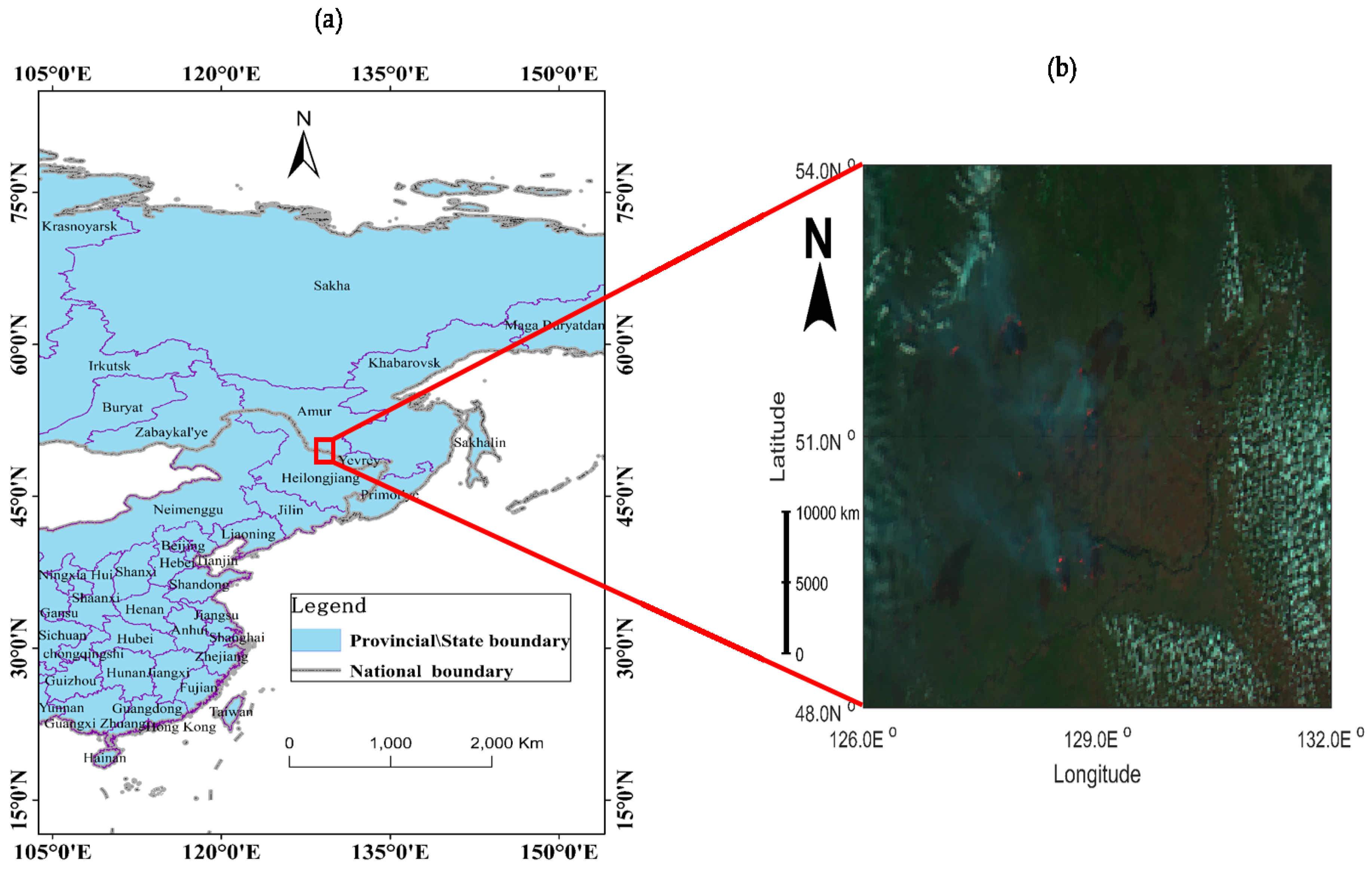
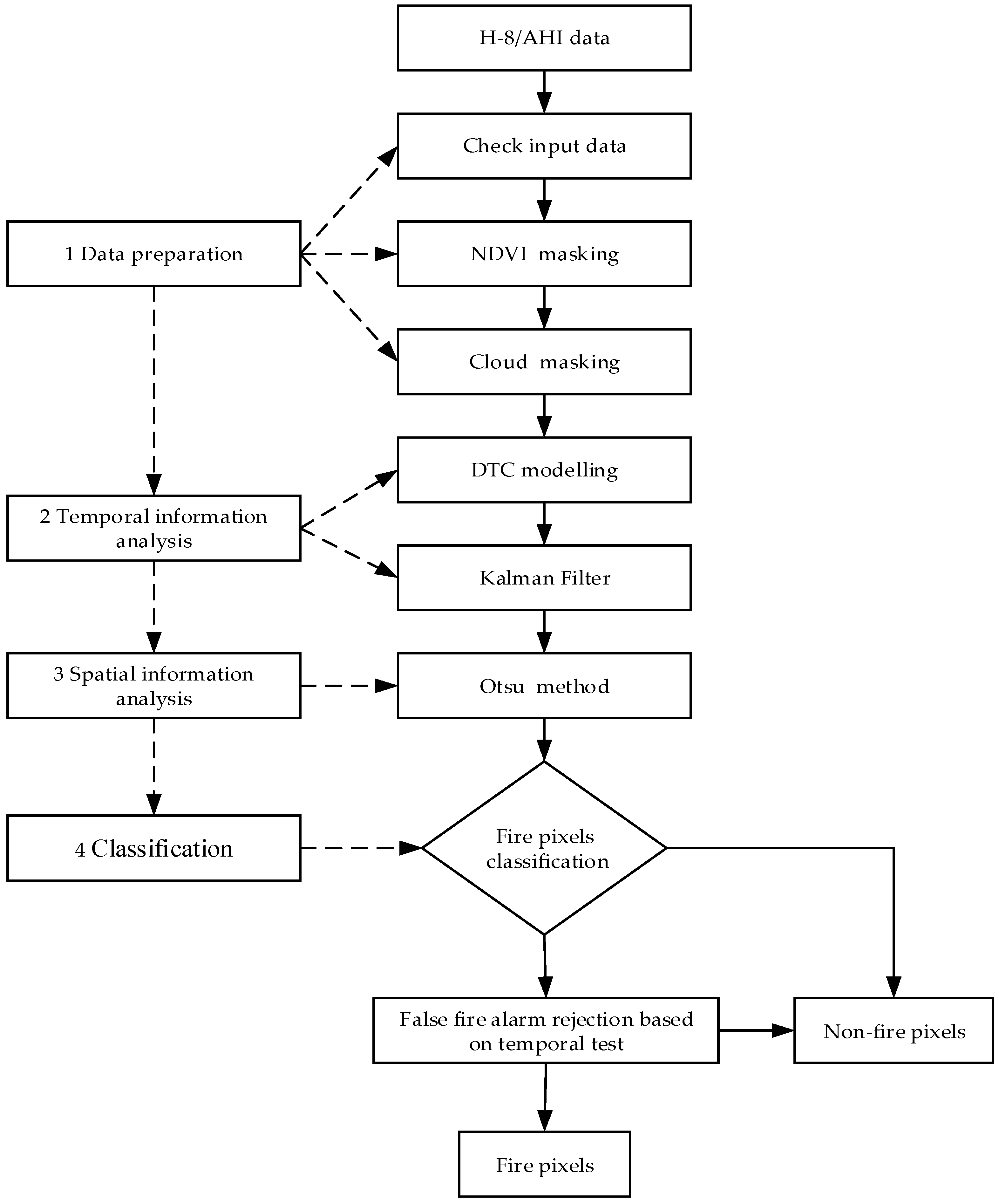
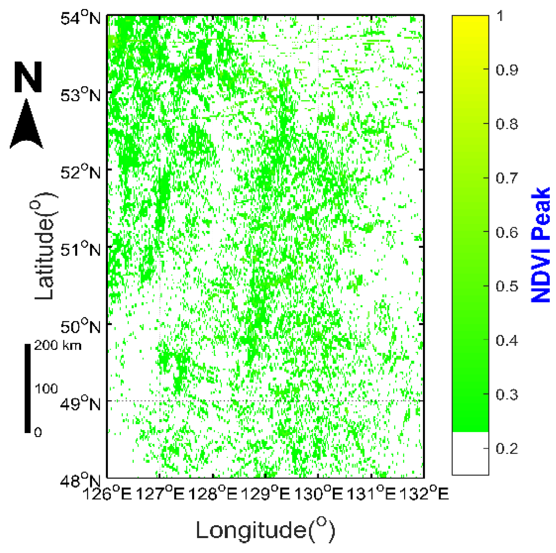
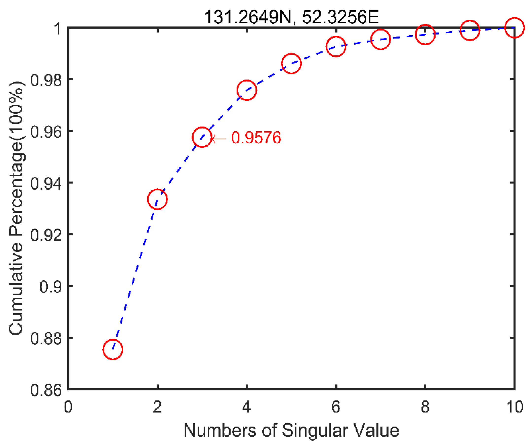
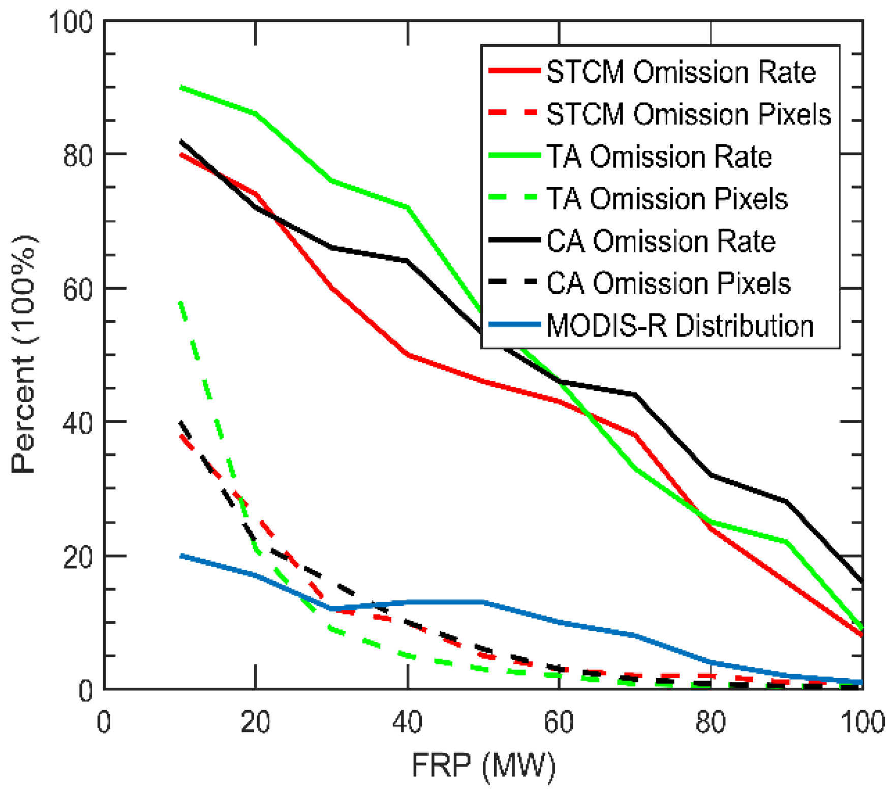
Table 1.
Case study fires used for evaluation of the spatiotemporal contextual model (STCM) algorithm.
Table 1.
Case study fires used for evaluation of the spatiotemporal contextual model (STCM) algorithm.
| Fire Case | Burned Area (km2) | Duration | Geographic Coordinate Range |
|---|---|---|---|
| Bilahe | 115 | 2 to 6 May 2016 | 49°N–50°N, 123°E–124°E |
| Cross-border | 5625 | 2 to 14 May 2016 | 48°N–54°N, 126°E–132°E |
| Adelaide | 850 | 20 to 28 November 2016 | 34°S–36°S, 138°E–140°E |
| Tasmania | 1050 | 15 to 28 January 2016 | 41°S–44°S, 145°E–148°E |
Table 2.
Bands of Himawari-8 imagery used for hotspots detection.
| Band # | Wavelength (µm) | Spatial Resolution (km) | Unit | Detection Target |
|---|---|---|---|---|
| 2 | 0.51 | 1 | Unitless | cloud |
| 3 | 0.64 | 0.5 | Unitless | cloud/night/vegetation |
| 4 | 0.86 | 1 | Unitless | cloud/night/vegetation |
| 6 | 2.3 | 2 | Unitless | cloud |
| 7 | 3.9 | 2 | Kevin | fire/cloud |
| 14 | 11.2 | 2 | Kevin | fire |
Table 3.
Evaluation of relative accuracy of each brightness temperature (BT) fitting process using root mean square (RMS) error in comparision to raw BTs in middle infrared (MIR) and longwave infrared (LWIR).
Table 3.
Evaluation of relative accuracy of each brightness temperature (BT) fitting process using root mean square (RMS) error in comparision to raw BTs in middle infrared (MIR) and longwave infrared (LWIR).
| Fitting Technique | RMS Error (K) | |||||||||
|---|---|---|---|---|---|---|---|---|---|---|
| Number of Outliers | ≤30 | 30–60 | 60–90 | 90–120 | >120 | |||||
| Band | MIR | LWIR | MIR | LWIR | MIR | LWIR | MIR | LWIR | MIR | LWIR |
| RFA | 0.51 | 0.94 | 3.48 | 1.98 | 1.73 | 3.46 | 9.69 | 18.72 | 24.87 | 36.81 |
| IRFA | 0.51 | 0.33 | 0.93 | 0.87 | 1.32 | 1.03 | 3.87 | 7.98 | 14.28 | 17.96 |
| Contextual method | 0.51 | 0.48 | 0.53 | 0.45 | 0.67 | 0.56 | 0.64 | 0.64 | 0.72 | 0.83 |
| Number of samples | 38 | 2652 | 46,682 | 43,368 | 11,2596 | |||||
Table 4.
Evaluation of robustness to outliers of each BT fitting process using root mean square error in comparision to average contamination-free BTs in MIR and LWIR.
Table 4.
Evaluation of robustness to outliers of each BT fitting process using root mean square error in comparision to average contamination-free BTs in MIR and LWIR.
| Fitting Technique | RMS Error (K) | |||||||||
|---|---|---|---|---|---|---|---|---|---|---|
| Incidences of CSP < 1 | ≤30 | 30–60 | 60–90 | 90–120 | >120 | |||||
| Band | MIR | LWIR | MIR | LWIR | MIR | LWIR | MIR | LWIR | MIR | LWIR |
| RFA | 10.46 | 16.29 | 20.38 | 20.26 | 16.74 | 21.42 | 14.52 | 18.47 | 23.36 | 33.29 |
| IFRA | 8.31 | 11.74 | 18.01 | 18.54 | 13.25 | 17.28 | 14.52 | 16.20 | 14.27 | 22.36 |
| Contextual method | 22.29 | 26.88 | 20.36 | 24.88 | 36.47 | 36.90 | 38.24 | 36.27 | 29.83 | 36.87 |
Table 5.
Detection results of each fire detection method against simultanneous MODIS active fire product.
Table 5.
Detection results of each fire detection method against simultanneous MODIS active fire product.
| Fire Case | Commission Error (%) | Omission Error (%) | ||||||
|---|---|---|---|---|---|---|---|---|
| CA | TA | STCM | STCM2 | CA | TA | STCM | STCM2 | |
| Bilahe | 9.37 | 10.26 | 7.16 | 5.08 | 70.42 | 66.28 | 53.29 | 50.76 |
| Cross-border | 8.27 | 8.73 | 7.16 | 5.27 | 60.18 | 52.64 | 49.27 | 48.13 |
| Adelaide | 10.27 | 10.34 | 7.62 | 5.36 | 66.73 | 56.26 | 52.96 | 50.19 |
| Tasmania | 8.46 | 8.48 | 6.28 | 5.72 | 62.35 | 50.74 | 48.27 | 44.36 |
| Overall (A) | 9.09 | 9.45 | 7.06 | 5.36 | 64.92 | 56.48 | 50.95 | 48.36 |
| Overall (D) | 7.48 | 8.36 | 6.85 | 5.03 | 52.76 | 48.65 | 44.72 | 41.03 |
| Overall (N) | 10.7 | 10.54 | 7.27 | 5.69 | 77.08 | 64.31 | 57.18 | 55.69 |
“CA”, “TA”, “STCM”, and “STCM2” denote the results accuracy for contextual algorithm, temporal algorithm, STCM, and STCM after temporal test, respectively. “Overall (A)”, “Overall (D)”, and “Overall (N)” represent results accuracy for average, daytime, and nightime, respectively.
© 2018 by the authors. Licensee MDPI, Basel, Switzerland. This article is an open access article distributed under the terms and conditions of the Creative Commons Attribution (CC BY) license (http://creativecommons.org/licenses/by/4.0/).
Share and Cite
MDPI and ACS Style
Xie, Z.; Song, W.; Ba, R.; Li, X.; Xia, L. A Spatiotemporal Contextual Model for Forest Fire Detection Using Himawari-8 Satellite Data. Remote Sens. 2018, 10, 1992. https://0-doi-org.brum.beds.ac.uk/10.3390/rs10121992
AMA Style
Xie Z, Song W, Ba R, Li X, Xia L. A Spatiotemporal Contextual Model for Forest Fire Detection Using Himawari-8 Satellite Data. Remote Sensing. 2018; 10(12):1992. https://0-doi-org.brum.beds.ac.uk/10.3390/rs10121992
Chicago/Turabian StyleXie, Zixi, Weiguo Song, Rui Ba, Xiaolian Li, and Long Xia. 2018. "A Spatiotemporal Contextual Model for Forest Fire Detection Using Himawari-8 Satellite Data" Remote Sensing 10, no. 12: 1992. https://0-doi-org.brum.beds.ac.uk/10.3390/rs10121992
Note that from the first issue of 2016, this journal uses article numbers instead of page numbers. See further details here.