Post-Disaster Recovery Assessment with Machine Learning-Derived Land Cover and Land Use Information

Abstract

Post-disaster recovery (PDR) is a complex, long-lasting, resource intensive, and poorly understood process. PDR goes beyond physical reconstruction (physical recovery) and includes relevant processes such as economic and social (functional recovery) processes. Knowing the size and location of the places that positively or negatively recovered is important to effectively support policymakers to help readjust planning and resource allocation to rebuild better. Disasters and the subsequent recovery are mainly expressed through unique land cover and land use changes (LCLUCs). Although LCLUCs have been widely studied in remote sensing, their value for recovery assessment has not yet been explored, which is the focus of this paper. An RS-based methodology was created for PDR assessment based on multi-temporal, very high-resolution satellite images. Different trajectories of change were analyzed and evaluated, i.e., transition patterns (TPs) that signal positive or negative recovery. Experimental analysis was carried out on three WorldView-2 images acquired over Tacloban city, Philippines, which was heavily affected by Typhoon Haiyan in 2013. Support vector machine, a robust machine learning algorithm, was employed with texture features extracted from the grey level co-occurrence matrix and local binary patterns. Although classification results for the images before and four years after the typhoon show high accuracy, substantial uncertainties mark the results for the immediate post-event image. All land cover (LC) and land use (LU) classified maps were stacked, and only changes related to TPs were extracted. The final products are LC and LU recovery maps that quantify the PDR process at the pixel level. It was found that physical and functional recovery can be mainly explained through the LCLUC information. In addition, LC and LU-based recovery maps support a general and a detailed recovery understanding, respectively. It is therefore suggested to use the LC and LU-based recovery maps to monitor and support the short and the long-term recovery, respectively.

1. Introduction

Disaster risk management (DRM) comprises four distinct phases: Mitigation, preparedness, response, and recovery. Post-disaster recovery (PDR) is generally described as the process of returning to a normal condition after a period of difficulties [1]. However, recovery has been recognized as a complex and arduous process that in minor cases can be evaluated in months or years, and in extreme cases in decades, mainly because of the involvement of various stakeholders and the multi-phase nature of the PDR process [2]. Recovery comprises four distinct aspects that partially overlap: The built environment that recovery is often reduced to, but also the social, natural, and economic aspects, of which each includes further subdomains [3].

Although large-scale natural disasters can extensively damage an affected area and community, disasters and the subsequent recovery processes also bring opportunities for disaster-stricken communities. Within a recovery process, pre-existing vulnerabilities can be identified and addressed, with the post-disaster window of opportunity allowing the central Sendai Framework pillar of Building-Back-Better to be realized [4]. The priority of the Sendai Framework in the recovery phase is enhancing disaster preparedness for an effective response to “Build Back Better” (BBB). BBB is the concept that uses the recovery process not only to build back an affected area to the pre-disaster situation through physical rebuilding, but also to improve living and environmental conditions through risk reduction measures, resulting in more resilient and sustainable communities [5,6]. BBB provides a holistic recovery framework that considers both physical and functional recovery, while conventional thinking of recovery is based on Building Back (BB) areas to the pre-disaster level, considering only the physical recovery. The additional functional recovery describes how a community is functioning after a disaster, which can only be observed indirectly in remote sensing imagery, e.g., the change of functionality of (critical) buildings.

After large disasters, a considerable amount of money from donors and governments is often made available to finance the recovery to reach the recovery goals [2]. During the recovery, its progress needs to be monitored to assess what has been achieved and where readjustment is required. Thus, recovery assessment is vital for policymakers and donors, while it also improves the transparency of the process, the capability of executing agencies for on-going works, and it supports auditing efforts and accountability [7]. Furthermore, the quality and the speed of the recovery process can be used as indicators of the resilience of an affected community [8]. Resilience can be assessed via the residual functionality after a disaster (robustness), and by the speed of functional recovery to a normal situation; i.e., pre-disaster norm or a new equilibrium. Besides, monitoring of risks is essential and is a continual process, since risks continually change. One of the main purposes of post-disaster risk assessment is to identify any secondary risks. Therefore, recovery assessment can also be used as a basis for effective post-disaster risk assessment [9].

Although a systematic assessment of the recovery process is important for all stakeholders, it has been described as the least understood phase of disaster management [10]. No comprehensive models exist to measure recovery over time [11]. Conventional recovery assessment studies focus on the built-up environment and short-term evaluation of damaged buildings and their recovery status, or on the community level through social audit methods [7]. The latter cover ground-based techniques such as household survey, which cannot cover all aspects of integrated recovery, specifically over large areas, while also being time- and money-consuming and prone to subjectivity [8]. Social audits are mainly used to collect and combine the data regarding the timing and the quality of the process, as well as people’s perception of the process. The result of those types of recovery assessment methods is normally qualitative reports with limited practical usability for decision makers [12,13].

Remote Sensing (RS) has been shown to be a cost-effective source of spatial information for all aspects of disaster risk [14]. The availability of remotely sensed datasets before and after an event, as well as growing image archives, also allows for an increasingly effective use of RS in recovery assessment. However, the utility of RS to support and monitor the recovery is the least developed application in the DRM cycle [15]. RS can greatly contribute to monitor and assess the recovery process through facilitating time-series analysis over large areas and at short intervals.

In RS-based recovery assessment most of the developed methods and data-types have focused on the physical recovery [15]. For instance, video data allow us to analyze the accessibility problems of remote places [16]. Brown et al. [7] used indicator-based methods based on Very High Resolution (VHR) satellite imagery combined with social audits for recovery assessment. Their indicators are mostly at building-level and thus expensive and time-consuming to collect, due to manual extraction from RS images, while lacking practicality, e.g., clean or dirty swimming pools. Although those indicators can be helpful to a limited extent, they do not reveal recovery information on a practical scale. Besides, the image analysis technique used (maximum likelihood classification) assumes a normal data distribution, which is not appropriate for VHR images [17]. Hoshi et al. [18] used a ground survey in combination with remote sensing, employing visual interpretation and binary classification methods to monitor post-disaster urban recovery.

Recent studies have focused on post-fire recovery using vegetation indices to evaluate greenness recovery from satellite imagery [19,20,21]. Thus, the few image analysis methods used for recovery assessment tend to be rather dated, not suitable for VHR imagery, and do not use suitable image processing developments (e.g., machine learning techniques). Also most of the current literature tends to be limited to a particular and relatively small area [22], which can limit the strength of the scientific findings since there is no consideration of spatial extrapolation or transferability of the method, while recovery information is commonly required for large areas, and generic rather than country-specific assessment methods are needed. Hence, there is a need to develop a more comprehensive RS-based methodology using recent image analysis methods.

Artificial Neural Network (ANN) and more recent Convolutional Neural Network (CNN) [23,24] has the ability to retrieve complex patterns and learning features from the data. CNN has shown advantages over other ML methods [25]; however, its hidden layer is a black box and the overall accuracy is highly dependent on the amount of training data. Moreover, CNN is not easy to use and computationally is expensive, that normally needs dedicated hardware to handle the process. On the other hand, recent studies show state-of-the-art Machine Learning (ML) methods such as SVM, a relatively easily implementable method, can handle learning tasks with a small training dataset (i.e., is the case of disaster situations), yet shows competitive results with CNNs [26]. The performance of SVM is good for complex datasets; such as urban-rural setting in developing countries, where the performance of random forest (RF) is data-dependent and mainly performs well for non-complex datasets [25,27].

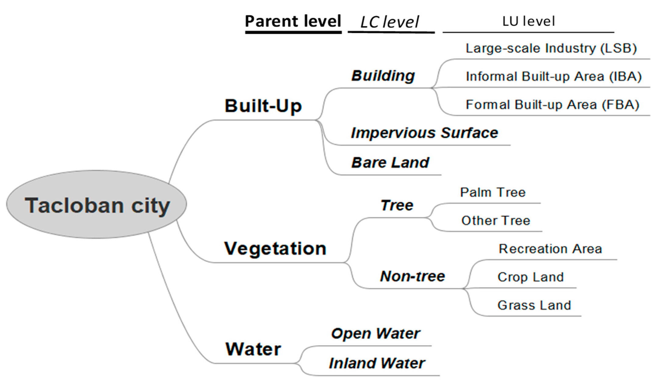
Disasters and recovery processes significantly influence land cover (LC) and land use (LU) [28]. LCLU information has been widely explored in different fields of remote sensing; however, the value of LCLU information has not been studied well in the recovery literature. Land cover and land use change (LCLUC) is a robust indicator with high explanatory power across the disaster-stricken area and over time, which also can be used to assess how well the affected area is recovered [10].

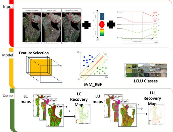
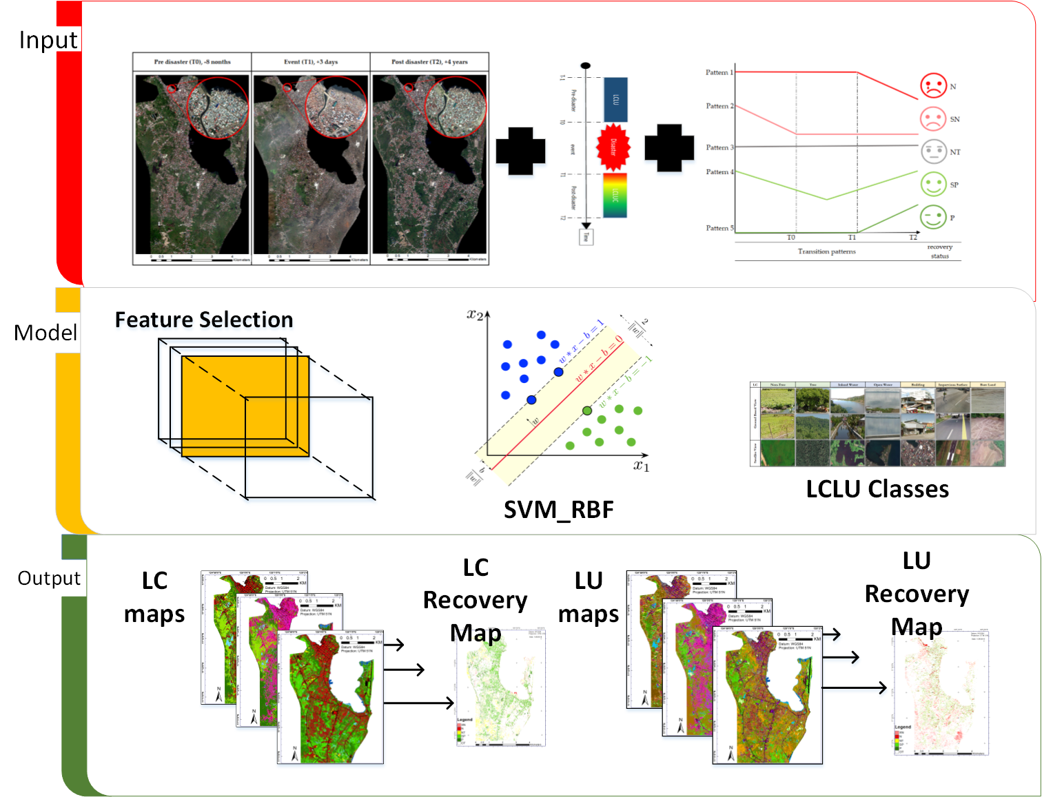
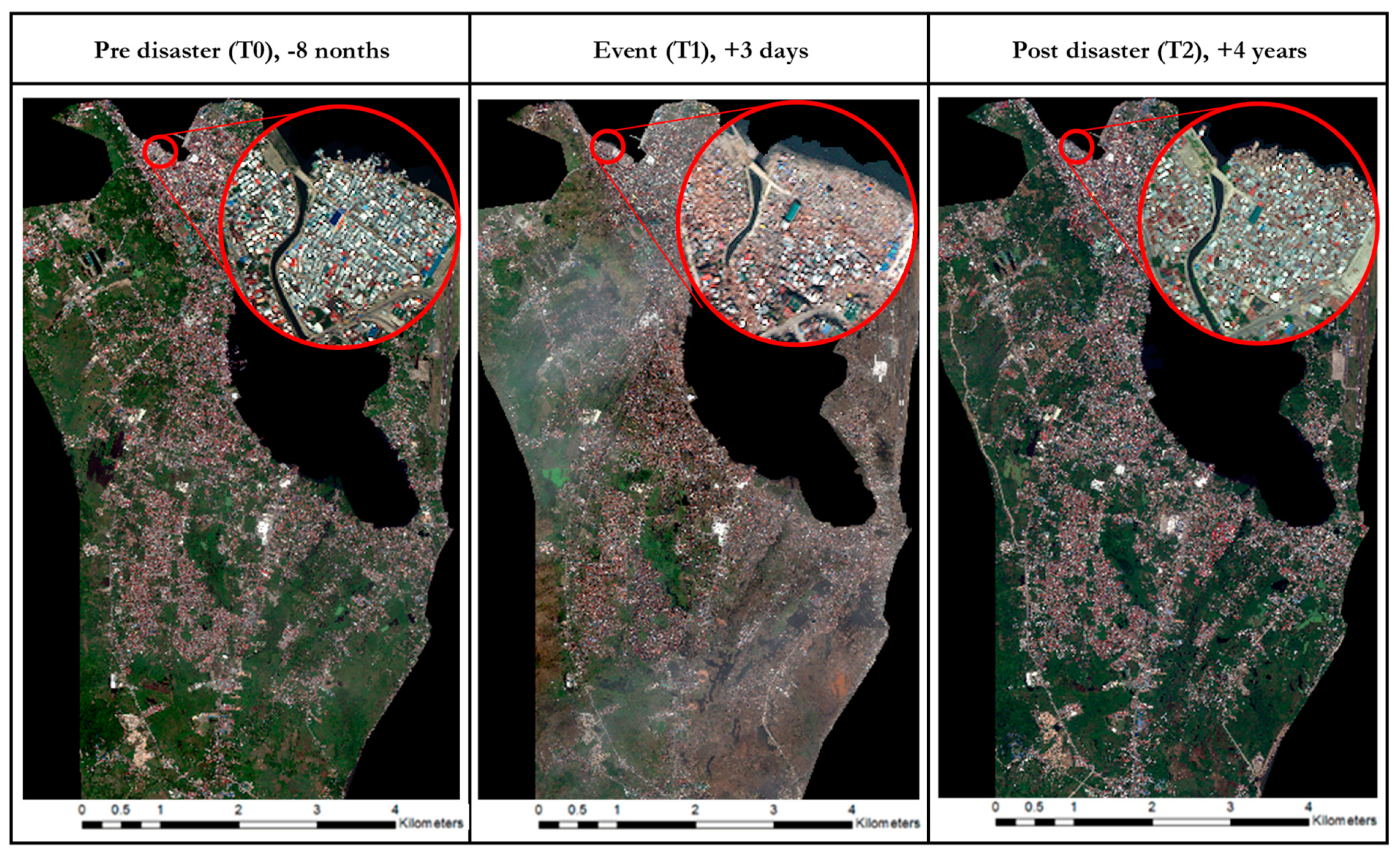
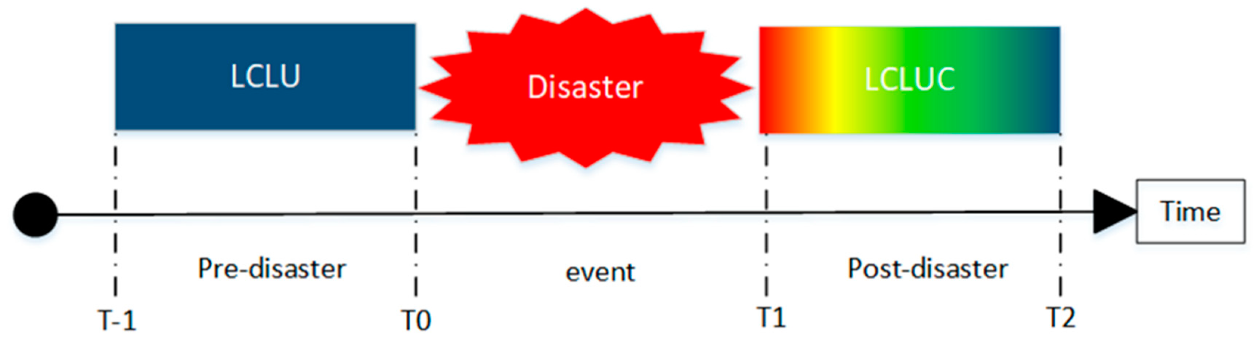
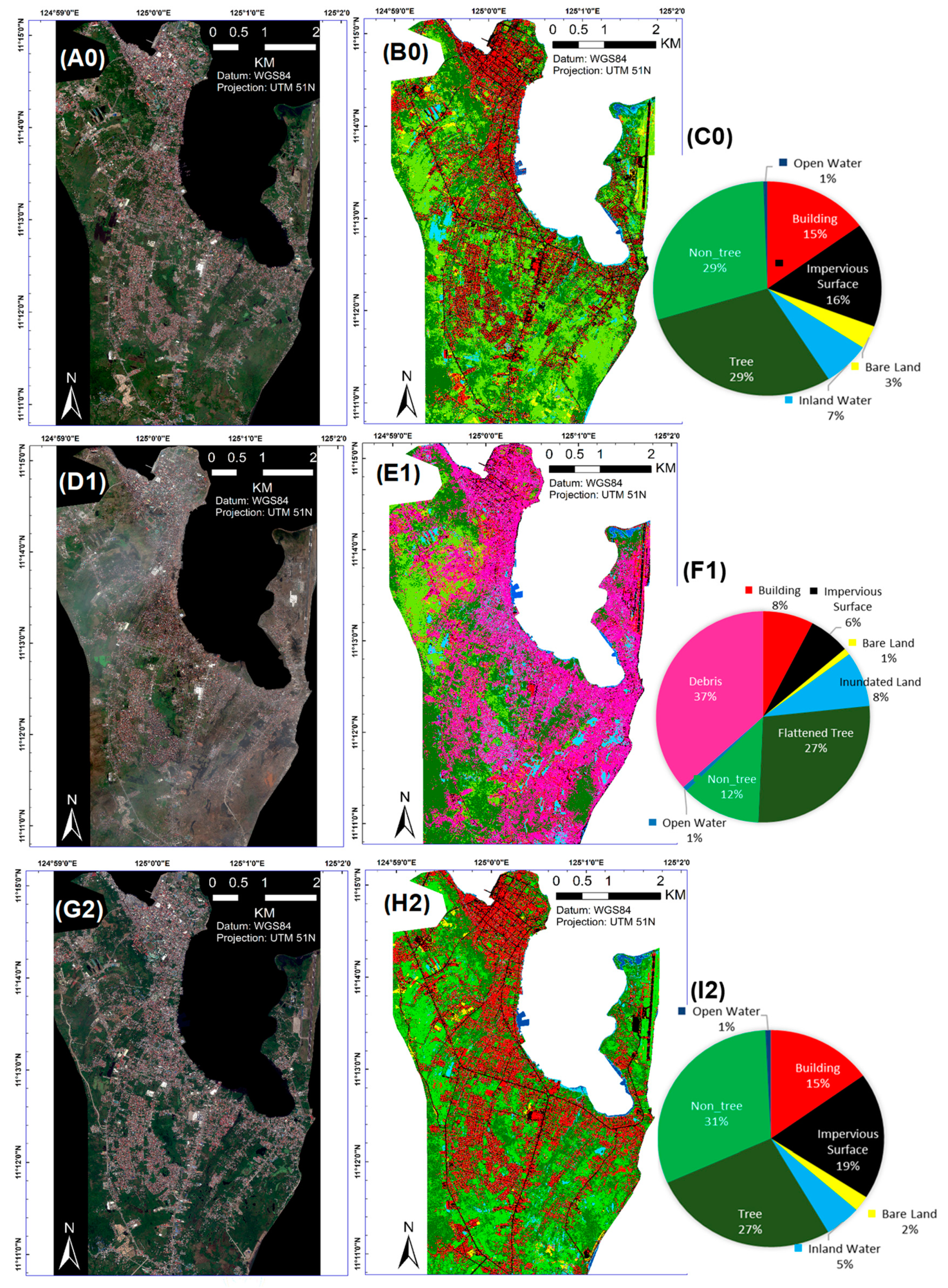
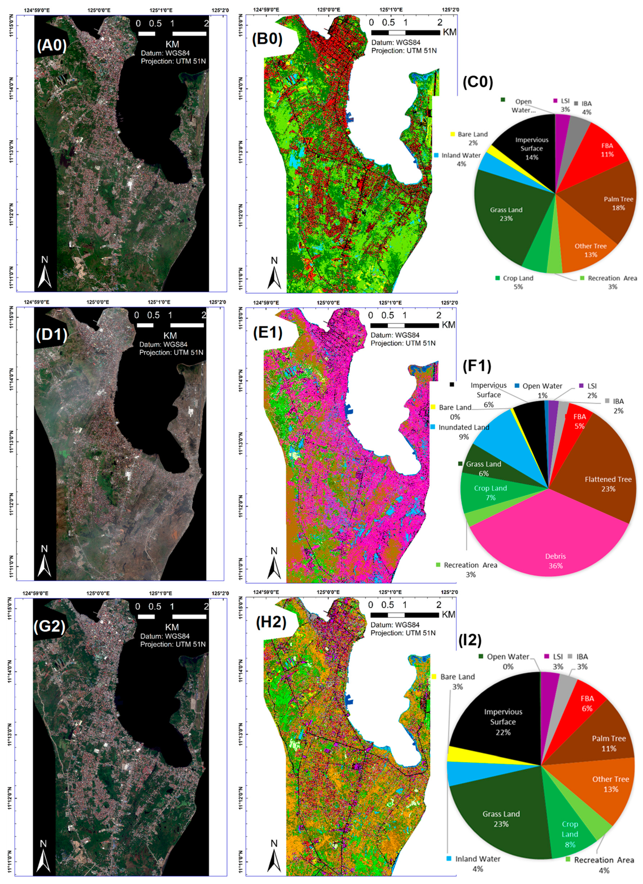
The aim of this paper is to investigate the utility of LCLUC information to assess PDR, using VHR satellite images and machine learning. For this, a new RS-based methodology was developed that gives value judgments on unique trajectories of changes; e.g., positive and negative recovery. Support Vector Machine (SVM) was used for the classification of three WorldView-2 images. The suitability of image features was investigated and those with high discriminative power were selected for the LC and LU classification task. A code was developed for the post-classification change assessment, based on which meaningful changes during the PDR process were mapped, i.e., LC- and LU-based recovery maps. Subsequently, the usefulness of LCLU information was discussed. The urban and rural area of Tacloban city in the Philippines was selected as a test, and PDR was assessed in the context of typhoon Haiyan, over a period of 5 years. Tacloban city was hit by Super Typhoon Haiyan on 8 November 2013, the strongest ever typhoon recorded worldwide that officially caused more than 5000 fatalities [29]. Tacloban city was selected for this purpose as it includes relatively complex land cover and land use patterns that are suitable to characterize PDR sectors (social, natural, economic, and built environment).

2. Materials and Methods

2.1. Test Area and Remote Sensing Data

Tacloban city is located in the Eastern Visayas (Figure 1). The eye of the typhoon passed just South of Tacloban city, causing massive destruction. Based on official news, just in the city itself 2678 people died (45% of the total number of fatalities in the country), and approximately 40,000 homes, representing 88% of all households, were demolished or damaged with the majority being informal coastal communities [30]. Three WorldView-2 images (see

Table 1. Description of data used.

ID	Acquired Date	Timeline	Satellite	MS Resolution	Description
T0	17 March 2013	8 months before Haiyan	Worldview-2, 8 bands {C, B, G, Y, R, RE, NIR1, NIR2}	2 m	Tacloban city, in the Philippines, Area~26 ${\mathrm{km}}^2$
T1	11 November 2013	3 days after Haiyan
T2	18 March 2017	4 years after Haiyan

) were used, acquired over Tacloban, 8 months before (pre), 3 days after (event), and 4 years after typhoon Haiyan (post), to study PDR assessment, based on the local knowledge of the two authors of this research (Figure 2).

2.2. Recovery Framework Based On LCLUC

To create the Conceptual Framework (CF), first a simple interaction of LCLU and disaster and subsequent recovery process was created (Figure 3). The underlying premise is that LC information predominantly relates to physical recovery, while LU change is more closely associated with changes in functionality of buildings and neighborhoods. The CF is based on common changes in a disaster-stricken area that can be described by LCLU, called Transition Patterns (TPs).

TPs are grounded in multi-temporal image analysis and are trajectories of changes, related to identical pixels in an n-timespan image set, where “n” in this research is 3 (the number of images). The state of the pixels is defined by predicted (LC/LU) labels. TPs trace the state of the pixels which implies a change; i.e., there are at least two different labels in one transition pattern; e.g., building (T0)—debris (T1)—building (T2).

The existing literature mainly considers a conventional perspective of recovery assessment via two simplistic recovery directions: Positive and negative recovery. Positive recovery occurs when a damaged structure is rebuilt to the pre-disaster level, whereas negative recovery is when it does not (e.g., an area is abandoned) [15]. Nevertheless, the recovery process is more complex, and needs a more comprehensive framework for a more nuanced and contextualized interpretation of recovery, when it comes to image-based recovery assessment. Hence, this paper considers five recovery classes, which are based on observation of most common changes related to before and after disaster (T0 and T1, respectively) that are linked through damage classes in the event time, all translated into TPs (Figure 4):

The definition of these classes is based on the most relevant LC- and LU-based TPs within three epoch spans; e.g., building-debris-building, and is based on the land use plan of the study area and the BBB perspective. Neutral recovery NT refers to those TPs that are not informative enough, as the classes are in the same parent level (Figure 5). For example, the TP building-building-impervious surface represents a change from building to another impervious surface from T1–T2, with both classes having the same parent class (built-up). Negative recovery (N) and positive recovery (P) refer to those TPs where the pixel-label at T1 remains the same as in T0, while showing change in T2. These changes, therefore, determine if the TP is negative or positive. Moreover, this definition is based on the assumption that if a pixel-label, e.g., building, can retain its state at the time of the event; e.g., building (T0)–building (T1), and survived the disaster, this signifies limited vulnerability to that specific hazard type, meaning that the class is either located in a safe zone or is well-adapted to that specific hazard. For example, building-building-bare land and grassland-grassland-impervious surface represent N and P (the classification of positive and negative changes is based on the land use plan of the study area), respectively. Classes SN and SP are the intermediary classes with inherent uncertainty. More information, such as additional satellite images, (multi) hazard maps of the area, or in-situ data, is required for SN and SP to be further accurately defined as N and or P. However, in the absence of such information, class SN tends to be negative, and SP tends to be positive. For instance, the patterns building-debris-bare land and building-debris-building exemplify the SN and SP, respectively. The last class, other transition (OT) comprises either minor and/or rare TPs (e.g., building-building-open water) or no change TPs (e.g., building-building-building), that is not the focus of this study. Using RS alone can impose uncertainty on the developed CF. For instance, building-debris-bare land (or impervious) may be seen as negative (no resources to rebuild, or people who moved away), but it can also be positive in the BBB sense, with the government preventing rebuilding in high-risk zones. However, the developed CF minimizes the inherent uncertainty by taking the land use plan of the study area into account.

2.3. LCLU Class Definition

Defining relevant classes is the basis for implementing the CF, as well as further classification and production of recovery maps. The most relevant classes were selected and categorized into three parent groups: Built-up, vegetation, and water. LC level and LU level classes were hierarchically defined based on the parent groups in the context of Tacloban city (Figure 5). Regarding class tree, those having a tree form are colloquially called palm trees, both in the study area and in the remote sensing domain [31].

In addition to LC and LU classes, it was necessary to study damage classes separately for the situation right after a disaster. Natural forces, e.g., heavy winds and a storm surges, heavily destroyed existing urban elements (almost all structures were washed away along the coastline). Therefore, there was a need to characterize the post-event damage classes. Regarding buildings, mainly two damage classes can be distinguished: Rubble and debris (Figure 6). However, at the city scale and with the spatial resolution of 2m, it was not possible to distinguish debris from rubble, as there are certain ambiguities between the classes due to structural debris and washed-up or wind-blown materials (Figure 6). Therefore, these two classes were merged into one class, debris, which consists of damage patterns related to a mix of wind-water borne objects, e.g., rubble, debris, woods, galvanized roof materials, etc. There are two other damage classes: Inundated land and flattened trees. Flattened trees are the trees in T0 and T2; however, they are mostly either inclined or flattened in T1 (Figure 7).

2.4. Framework Implementation

From a list of all possible TPs for the LC and the LU changes in the context of post-Haiyan recovery, the most relevant TPs were selected and illustrated in LC- and a LU-based CF (

Table 2. The LC-based conceptual framework for the post-Haiyan recovery process in Tacloban.

T0	T1	T2	Recovery Status
Non-tree (veg)	Non-tree (veg)	Inland water	N
Tree	Flattened tree	Inland water
Impervious surface	Debris	Tree	SN
Building	Debris	Tree
Tree	Flattened tree	Non-tree	NT
Impervious surface	Impervious surface	Building
Building	Debris	Building	SP
Impervious surface	Debris	Building
Impervious surface	Debris	Impervious surface	P
Non-tree (veg)	Non-tree (veg)	Impervious surface

and

Table 3. LU-based conceptual framework for the post-Haiyan recovery process in Tacloban.

T0	T1	T2	Recovery Status
Informal built-up area	Debris	Informal built-up area	N
Formal built-up area	Debris	Informal built-up area
Grass land	Flattened tree	Palm tree
Palm tree	Flattened tree	Palm tree	SN
Crop land	Flattened tree	Crop land
Formal built-up area	Debris	Bare land
Formal built-up area	Debris	Impervious surface	NT
Formal built-up area	Formal built-up area	Impervious surface
Other tree	Flattened tree	Palm tree
Formal built-up area	Debris	Formal built-up area	SP
Impervious surface	Debris	Formal built-up area
Formal built-up area	Inundated land	Formal built-up area
Crop land	Debris	Recreation area	P
Informal built-up area	Debris	Formal built-up area
Large-Scale industry	Debris	Large-Scale industry

, respectively). The recovery statuses were defined based on the land use plan of the study area in Tacloban after Typhoon Haiyan, which is scheduled to be completed in 2025 [33].

2.5. LCLU Mapping by Support Vector Machine

A Support Vector Machine (SVMs) is a non-parametric classifier that has been used to handle complex multi-class learning tasks with a small amount of training samples, and which produces competitive results [34], while also being capable of handling high dimensional data [35]. The wide use of the SVM classifier has been apparent in urban and vegetation related studies both in LC and LU classifications [35], making it one of the most suitable classifiers in the urban-rural context.

The variability of urban-rural setting in Tacloban’s landscape required a classification algorithm equipped to deal with complex relationships between spectral information and land surface conditions, while being robust with a small training data set. SVM is also known to be specifically well-suited for applications of multispectral imagery [36]. It is less data intensive compared to other machine learning algorithms such as Neural Networks, which require a large amount of training data [35]. In comparison with other methods such as backpropagation neural networks, SVMs can yield competitive accuracy [35].

For nonlinear decision surfaces, a kernel function was introduced by [37]. The present paper examined RBF (Radial Basis Function), linear kernels, and related parameters (C and γ) [38]. A grid-search using a cross-validation approach has been suggested as the most effective method to optimize the RBF parameters [39]. To facilitate the procedure, R package ‘e1071′, which was implemented in the LIBSVM library by Chang and Lin [40], was employed. Exponentially growing sequences of C and γ was used to identify the best parameters, for linear and RBF kernels along 2d, where d = {−5, −4, …} for γ and d = {5, 6, …} for C (

Table 4. The definition of grid search space for tuning the hyper-parameters support vector machine (SVM).

Classifier	Parameters	Grid-Search Space		Description
SVM	C	$2^5 to 2^{10}$		Regularization parameter which has a high impact on the generalization performance of the classifier.
		logarithmically spaced
	γ	2−5	to 20	Regularization parameter in RBF kernel with a high impact on the performance of the kernel.
		logarithmically spaced

).

2.6. Utilization of Image Features and Spectral Indices

Since some of the LU classes need a high semantic definition (e.g., informal built-up area), and also to decrease the spectral complexity of some similar classes (e.g., impervious surface and bare land), image-features, i.e., grey-level co-occurrence matrix (GLCM) and local binary pattern (LBP), as well as spectral indices such as NDVI were extracted. The GLCM and LBP, due to their discriminative power and computational simplicity, have been reported as the most useful features for urban studies [34]. Texture features were extracted with different lag distances and windows sizes (

Table 5. Extracted features from the multispectral image.

Type of Feature	Features Count	Description
Original bands	8	reflectance values of multispectral image (b1: b8)
Spectral indices	18	spectral indices
Local Binary Pattern	186	LBPR=2:4,P=6:12
GLCM	256	GLCM textural measures calculated for multispectral bands

). There are eight types of GLCM features (mean, contrast, angular second moment, variance, dissimilarity, correlation, homogeneity, and entropy), of which not all are useful and some are highly correlated, resulting in redundancy [41]. In addition, 18 different types of spectral indices from the most recent literature (mostly using WorldView-2 imagery) were used to help the classification task.

To reduce redundancy and to increase the effectiveness of the classification task, feature selection (Hilbert–Schmidt independence criterion (HSIC)) was employed. HSIC selects the most informative image-features, reduces computational costs and avoids over-fitting [42].

The overall, user, and producer accuracy (OA, UA, and PA, respectively) of the classification task were calculated. A common strategy for sampling methods was used based on a stratified random sampling and implemented by CARET package in R. 75% of the data was used for training the classifier and 25% for testing the accuracy of the classifier. Reference data were obtained using visual interpretation [43]. Seven LC and twelve LU classes were considered for the accuracy assessment with the minimum of 500 sample pixels of each class [44]. Visual interpretation was used based on multi-source data: Google Earth Pro, OpenStreetMap (OSM), Google Street View (GSV), and panchromatic bands of WV-2 imagery, to obtain training and test samples.

2.7. Recovery Maps

The recovery maps were based on the implemented CF and the LCLU classified maps. To create the recovery maps, first LC and LU maps from three time-spans (T0, T1, and T2) were stacked and then, for each map, the state of identical pixels was investigated. The same was done for all pixels in the classified images, and all possible TPs were identified. In this study, a code in R was developed to identify all possible TPs and to further select TPs based on the implemented conceptual framework (see Table 2 and Table 3).

3. Results and Analysis

3.1. Utility of Selected Features for LCLU Classification Tasks

As the result of feature selection, a combination of SVM+GLCM+NDVI2 (19 out of 302 features) and SVM+LBP+NDVI2 (23 out of 282 features), with an RBF kernel was selected to be applied to the study area to produce the LC and LU classification maps, respectively. From 18 different spectral indices, NDVI2 was selected as the most important spectral index. To differentiate non-built up areas from vegetation areas, NDVI2 showed a good discriminative power. An experiment to explore the effect of varying the window size of the extracted GLCM features on the LC classification result was conducted (windows sizes: 3 × 3, 5 × 5, 7 × 7, 9 × 9, and 15 × 15) and the most important GLCM measures were selected. For the LC task, increasing the window size results in a corresponding decrease in the overall accuracy. This is sensible, as detection of simple LC classes does not require abstract definition like informal built-up area from a large context [34]. Here, the GLCM variance and contrast measures of the first five bands of WV2 imagery with the window size of 3 × 3 were selected for the LC classification task. For LU classification, $LB{P}_{R=3,P=12}$, among many combinations (see: Table 5), was selected as the most informative feature set. The selected LBP in combination with NDVI2 was applied in the study area for LU classification task.

3.2. LCLU Accuracy Assessment

In general, for both LC and LU classification, SVM performed better for pre- and post-disaster compared to the event time. Regarding LC, the overall accuracies (OA) for T0 and T2 were 89.4% and 90.8%, respectively, while for T1 it was 82.2% (

Table 6. Comparison of LC classification accuracies for pre-event and post-disaster situations. User and producer accuracies and corresponding errors are computed across the study area by combining the confusion matrices of T0, T1, and T2.

Class	Pre Disaster (T0)			Event (T1)			Post Disaster (T2)
	Accuracy			Accuracy			Accuracy
	UA%	PA%	OA%	UA%	PA%	OA%	UA%	PA%	OA%
Building	95.5	83.8	89.4	68.0	55.0	82.2	82.2	94.2	90.8
Impervious Surface	83.8	96.3		82.0	68.8		84.3	99.5
Bare	88.0	83.4		76.9	50.2		98.0	62.3
Inland Water	87.3	90.3		95.2	94.2		98.8	99.9
(Flattened) Tree	77.9	88.9		83.1	96.1		96.5	92.9
Non_tree	93.5	85.2		89.5	61.0		92.7	90.9
Debris	-	-		64.4	87.7		-	-
Open Water	99.8	96.5		98.5	100.0		98.3	98.9

). The UA of the classes building and debris are comparatively low at 68% and 64.4%, respectively, which highlighted the error of commission in these two classes and the related uncertainties. There was also a relatively high commission error for the building and impervious classes, ranging from 4.5% and 16.2% in T0, and 32% and 18% in T1, to 17.8% and 15.7% in T2, respectively. This confusion was unavoidable due to the presence of concrete and asphalt roads, making it difficult to be differentiated. SVM + LBP + NDVI2 was applied to the whole study area to create LU classification maps with the OA of 76.3%, 69.9%, and 77.8% for T0, T1, and T2, respectively (

Table 7. Comparison of land use classification accuracies, user and producer accuracies, and corresponding errors are computed across the study area. LSI: Large scale industry; IBA: Informal built-up area; FBA: formal built-up area; PT: Palm tree; OT: Other tree; RA: Recreational area; CL: Crop land; GL: Grass land; IL: Inundated land; BL: Bare land; IS: Impervious surface; OP: Open water: Debris.

T0, T2 Class	Pre Disaster (T0)			Post Disaster (T2)			Event (T1)			T1 Class
	Accuracy			Accuracy			Accuracy
	UA%	PA%	OA%	UA%	PA%	OA%	UA%	PA%	OA%
LSI	88.28	59.68	76.3	84.18	86.59	77.8	77.7	77.2	69.9	LSI
IBA	76.74	81.04		93.66	59.7		97.6	37.0		IBA
FBA	53.74	90.83		69.83	72.71		68.3	39.1		FBA
PT	66.08	93.43		58.05	56.56		84.6	83.5		FT
OT	64.36	42.06		75.26	82.83		38.3	86.5		D
RA	91.82	68.83		97.15	73.77		64.4	19.1		RA
CL	72.83	73.16		80.7	43.21		50.1	85.0		CL
GL	66.75	65.62		58.22	86.16		40.5	33.4		GL
IW	97.19	92.35		96.2	99.14		84.4	94.5		IL
BL	94.98	75.11		94.46	73.71		87.4	45.9		BL
IS	79.47	82.7		62.65	95.69		74.5	69.6		IS
OP	100	98.92		99.26	98.53		98.6	99.1		OW

). Table 6 and Table 7 present the UA and PA for LC and LU over three epoch spans, respectively.

3.3. Visualization of Classified Maps

Figure 8 shows the LC maps and related pie charts. Buildings covers 15%, 8%, and 15% of the area in T0, T1, and T2, respectively. This implies that almost all buildings are reconstructed within 4 years after the typhoon, which also can be seen by visual interpretation of the imagery. The above-mentioned rebuilding can be considered a positive sign of recovery. However, more information is needed to better characterize the recovery status. Impervious surface shows an increase of 3% in T2 compared with T0. This also can be visually seen in the imagery, where, for instance, a new national road is constructed in T2 in the Western part of the city. For the vegetation category, the area covered by trees decreased by 2% in T2 as opposed to T0 while, conversely the area of non-tree vegetation increased by 2% in T2 against T0. Considering the damage classes in the disaster situation (T1), 37% of the area is occupied by different types of debris, while 8% of the land is inundated, and 27% of the land is covered by flattened tree. The damage classes show extensive destruction in Tacloban city, leading to a massive human and property loss [31].

Figure 9, on the other hand, shows the LU related pie charts. In the sub-building category, the size of LSI (large scale industry) remained the same in T2 compared to T0 (3%), though it shows a very small decrease of only 1% to 2% in T1, which could be an indication of good business recovery [33]. The area covered by IBA (informal built-up area) declined from 4% (T0) to 2% (T1). The typhoon completely destroyed some of the informal areas in Tacloban city [12]. Although the IBA increased again from 2% to 3% by 2017 (T2), it is not a good sign of the recovery process, since it re-establishes the pre-event high risk situation. The FBA (formal built-up area) shows a decrease of 5% in T2 as compared to T0. This is related to some areas that have been abandoned, and could also be partially related to the uncertainty in the classification of FBA in T2 as discussed earlier (Section 2.3). The size of covered land by palm trees shows a decrease from 18% in T0 to 11% in T2. This is in accordance with the comprehensive land use plan (CLP) of Tacloban city that called for a reduction in palm trees by almost half, and the time required for the growing of a new palm tree [12]. With regards to non-tree subclasses at LC level, the recreational area increased from 3% in 2013 to 4% in 2017. Moreover, the images show an approximately 3% increase in cropland between 2013 and 2017. The increase in recreational area is a good sign of recovery, as the size of the recreational area is also planned to be increased in the CLP [33]. However, the increase in cropland is not necessarily a sign of positive recovery, since the CLP called for a reduction in cropland. On the other hand, palm farmers have to replace the destroyed palm trees with other crops in order to generate income (cash crop).

3.4. Recovery Maps

Figure 10 shows the LC and LU recovery maps. The LC recovery map (Figure 10A) is dominated by green (positive recovery), while the LU recovery map (Figure 10B) overall contains more red (negative recovery). This difference is mainly related to the transition class SP (green) in the LC recovery map, while in LU recovery map transition class SP is mostly transformed into N and SN (red). For instance, TP building-debris-building (green) in LC is transformed to IBA-debris-IBA (red). Furthermore, the different TPs are selected in the LU CF compared to the LC CF (Section 2.4), and thus in the related recovery maps. When it comes to areas covered by transition classes SP and SN, the result of the LU recovery map is more specific and represents a more realistic recovery status as LU provides a more accurate information in those transitions compared to LC information.

Moreover, LC information is sufficient to characterize some classes and related TPs. For instance, the new national road in the Western part of the area is well-captured by the LC-based recovery map, see Figure 11F. Usefulness of LC information is also exemplified in Figure 11E, where a parking lot is added to a commercial building. Additionally, Figure 11D shows a potential positive recovery that has not been captured by both recovery maps, where a road is under construction, highlighting lack of image data, e.g., image data from 2018, to track some specific TPs which cannot be grasped by only a 3-epoch recovery map. Thus, a careful selection of satellite images is needed when it comes to RS-based recovery assessment.

4. Discussion

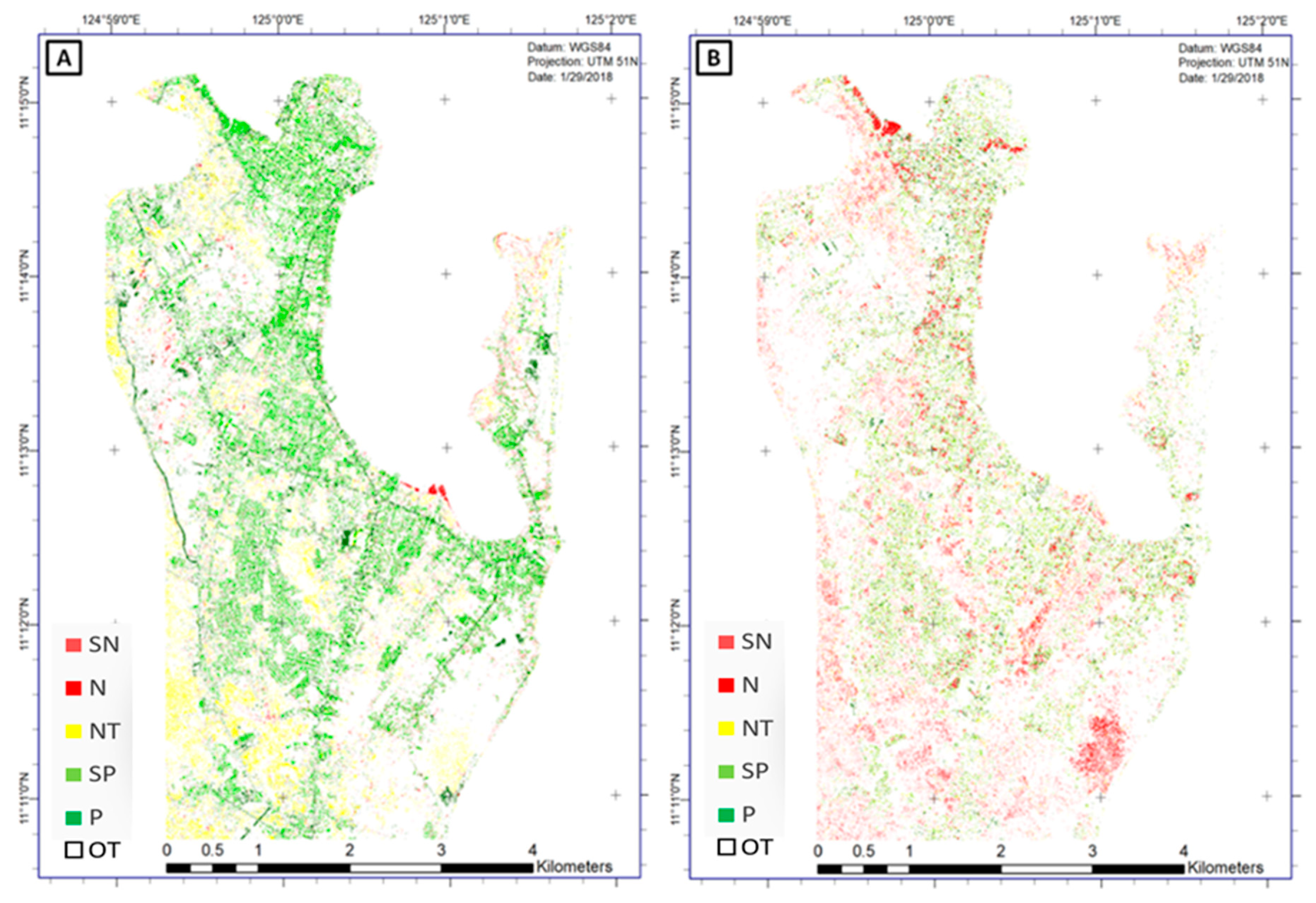
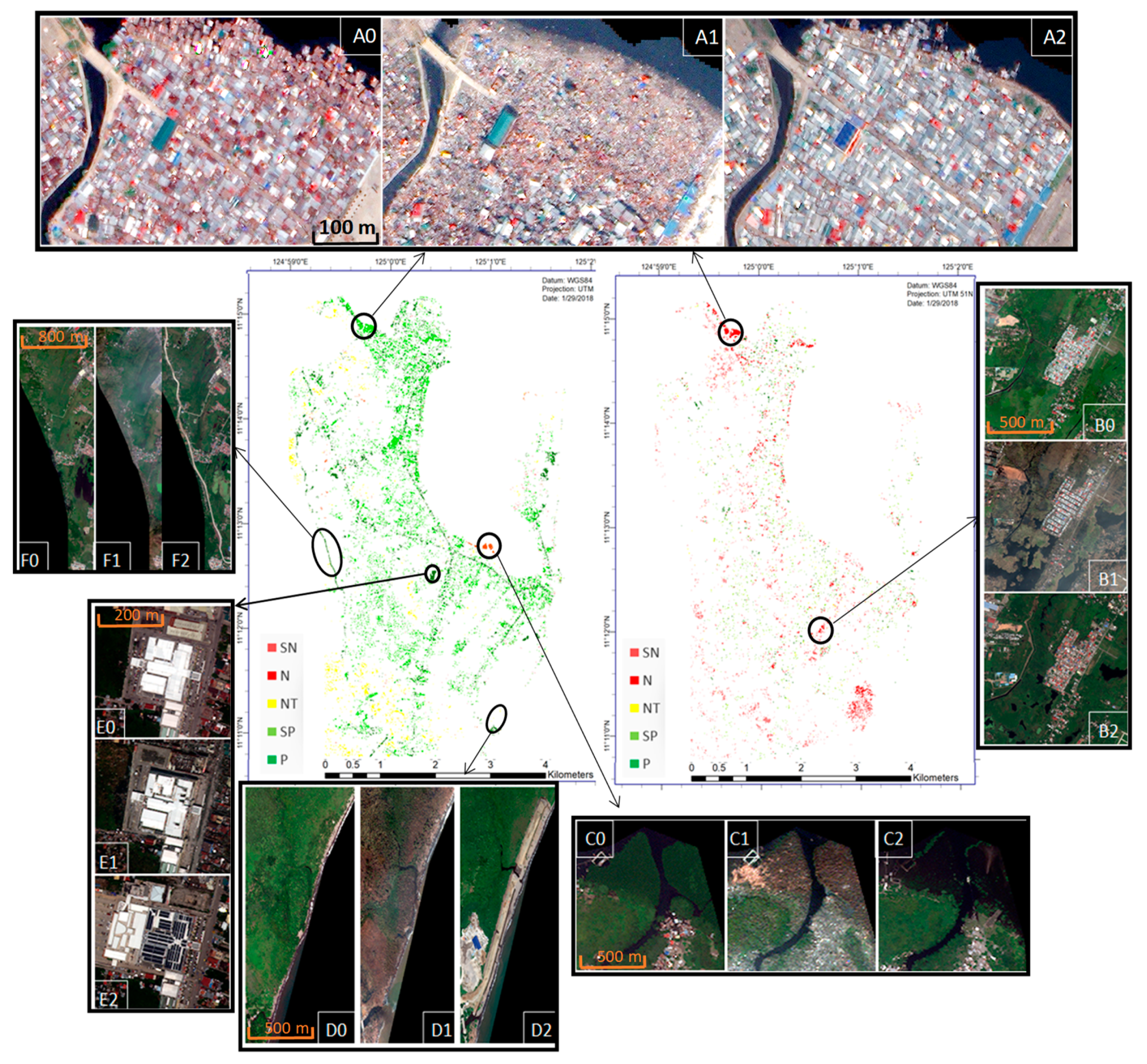
This research investigated the usefulness of LCLUC information through an RS-based CF for post-disaster recovery assessment. The developed CF largely captures the recovery process within three time steps. The CF is helpful for understanding the recovery processes and also for generating associated change maps. In the light of the CF, both physical and functional recovery were explored, leading to a holistic understanding of the recovery process. This study confirmed the initial hypothesis and showed that the LC-based recovery map primarily reveals physical aspects of recovery, while also being capable of generating a quick and reliable recovery insight over large areas. The LU-based recovery map, on the other hand, is more closely linked with the functional recovery assessment, where for instance changes in cash crop types (palm tree to crop land) and the state of residential areas (IBA to FBA) are influential factors to characterize PDR. However, in order to increase the generalization capacity and to support a deeper understanding of the recovery process, the CF could be refined by additional contextual factors (e.g., socio-economic data) of the affected area corresponding to each image.

Since providing LC information is easier and cheaper than LU, LC can serve as a basic layer that provides insights in the early stage of recovery process, with accurate results over large areas. LU-derived information can then be more effectively used in areas of uncertainty, or where more detailed information is required. Moreover, in the LC recovery map it is observed that the areas belonging to the classes SP and SN are the areas of extensional uncertainty, which ultimately need to be defined as N and or P. Overall, LC information is helpful for large areas, providing information on short-term recovery, while LU information is more helpful in a focused target classification for some specific aspects of recovery (e.g., economic recovery) and for some specific regions, allowing for detection of medium to long-term recovery activities.

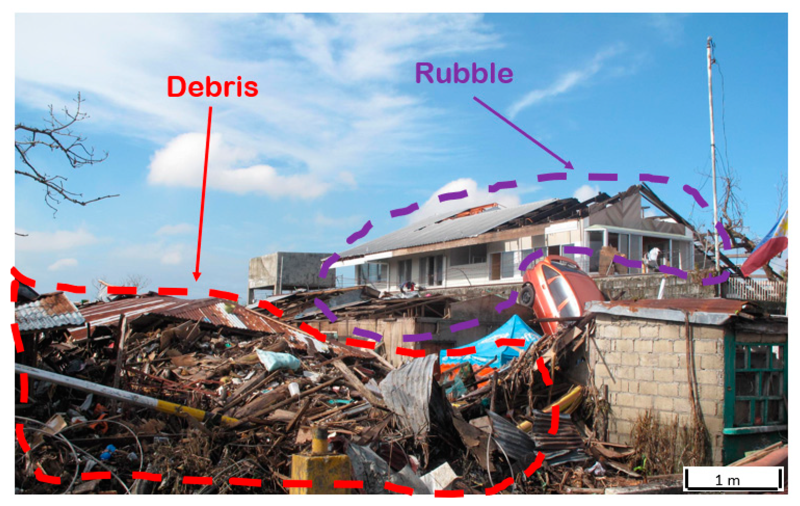
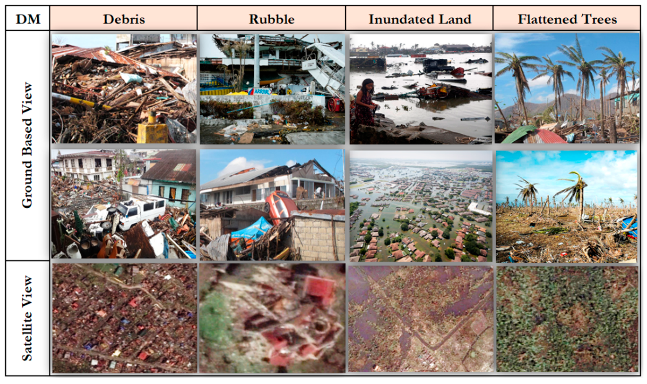
Damage estimation is critical in the relief and recovery process, and understanding and measuring damage types (structural and nonstructural damage) is an important step towards understanding and measuring the recovery process. Although the classifications of the T1 image showed high accuracy, complexity, and heterogeneity of the scene 3 days after Super Typhoon Haiyan [45], combined with the large and diverse number of classes involved in the LC and LU maps (7 and 12 classes, respectively) [46] and the relatively modest spatial resolution of the images (specifically for detailed urban mapping; 2 m) to differentiate the rate and type of damage [47], led to an overestimation of the area covered by debris (almost 37% of the area in T1). The uncertainty affected all TPs in the recovery maps that contain debris which might suggest a higher level of damage than in reality, and in turn a better recovery assessment. The most important TP, building, debris, building, played a significant role in the LC recovery map, resulting in a more greenish map (indicating positive recovery), which partly reflected the real recovery situation in Tacloban. It is recommended for future studies to differentiate better between structural damage and other objects next to buildings or on top of streets (in this case objects such as moved cars, vegetation matter, etc., moved and deposited by heavy wind and water). Using a higher spatial resolution and adding oblique images of buildings (for example acquired by UAV), [48] in combination with deep learning methods can improve the classification of event image and eventually the recovery maps [25,49]. Damage degrees (severity of damage) vary across space and time, yet the corresponding uncertainty was not fully captured in the developed framework, i.e., in T1 and T2, where the degree of damage and rebuilding are assumed to be discrete. Nevertheless, different levels of damage exist, ranging from complete collapse to cracks in the building roof or façades [50,51], as well as different degrees of rebuilding [52].

CNN, in the work of Mboga et al. [34], leads a better classification of built-up classes as compared to SVM, where accuracies were competitive but the computational costs differed substantially. Besides, CNN requires huge training data, which are difficult to supply in a case where ground truth data are limited (e.g., in disaster situation for damage classes), and also it is computationally very expensive without dedicated hardware (e.g., GPU) [24], makes it less suitable as a classifier compared to SVM in the current research. Regarding the vegetation-related classes, the results of SVM confirmed those of Ozdogan et al. [53] over a large area, while not corresponding well with the results of Mathur et al. [54] at a more local scale. Uncertainty due to mixed-unit classes in the LU level is conditional upon the temporal and spatial variability of the spectral signature of the classes in question. Thus, a careful definition of mixed-unit classes at LU level would improve mapping of the heterogeneous scene, as mentioned in the work of Herold et al. [55]. Moreover, appropriate images must be available for the temporal approach to provide a complete vegetation phenology of the focus crop types, before, and delayed vegetation phenology, after a disaster [53]. Therefore, understanding vegetation-related changes after a disaster requires an understanding of the regular vegetation phenology prior to the disaster. Hence, considering more than the 3-time steps used in this study would greatly benefit vegetation recovery assessment. Moreover, to capture a fuller view of recovery assessment, this study suggests using of another image within a range of 3-months after a disaster. This would effectively support quick monitoring needs of stakeholders and allows a better estimation of debris volume and removal [56].

Recovery information is specific for a disaster-stricken area and is related to a certain period. Thus, recovery is a geographic phenomenon that is made up of transition patterns tied to geographic objects [57]. When recovery information about coverage, capacity, and connectedness is needed at a city level, recovery information can be aggregated. It is also clear that with the high potential and flexibility of TPs to create recovery maps, the mapping approach could potentially be misused and manipulated. As shown with the divergent LC and LU-based recovery maps, it is possible to create assessments that emphasize the positive side of recovery, such as by focusing on physical recovery.

The LCLU and recovery maps are necessary to support decision making, planning in support of post disaster recovery, and eventually post-disaster risk management [11]. For instance, the maps can be used to decide if a highly exposed informal settlement should be relocated to a less hazardous area. This information could be used to guide municipalities and local authorities to properly allocate resources, including funding and technology for recovery projects in the long term within the concept of BBB, while they could also be used to evaluate land use plans in a timely manner [7]. Image-based recovery maps are also far less expensive tools compared to fully ground-based surveys and social audits. Image-based recovery maps provide detailed insights for donors to track the impact of their investments in the affected areas. Besides, recovery maps can indicate where ground-based techniques might be relevant to gain more detailed insights (e.g., areas of uncertainties).

5. Conclusions

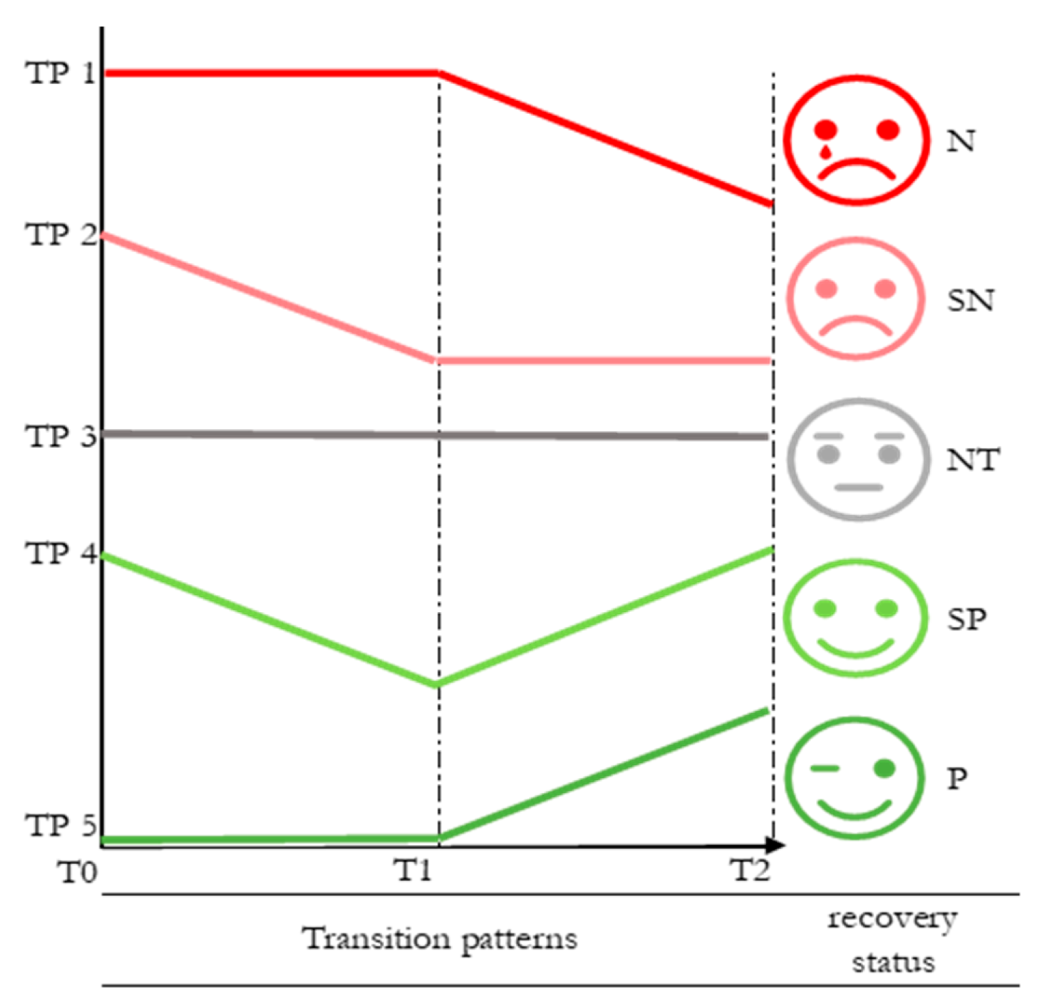
We lack standard methods for recovery assessment, where existing methods are either (i) limited to physical reconstruction detection, or (ii) qualitative/anecdotal. The contribution of the paper is to provide a conceptual framework for a rigorous LCLU-based recovery assessment. The developed CF for image-based recovery assessment introduces a nuanced definition of recovery based on TPs, which are categorized into five groups: Positive, slightly positive, neutral, slightly negative, and negative recovery. It was found that some TPs can specifically characterize short- and some long-term recovery. A general understanding of the recovery can be provided by the LC-based recovery map alone, which is cheaper and easier to produce and normally has a higher accuracy than LU information. The ML method was used (SVM) and could be simply implemented by local authorities and does not require huge computational resources (as compared to deep learning methods).The LC-based recovery map can provide planners with basic information about the ongoing recovery, and reconstruction planning could entirely consider the pre-disaster situation and deal with the dramatically changed situation after the event. However, the amount of uncertainty in the LC- based recovery map (SN, SP) requires more detailed information to be further characterized (as N or P). LU information and the LU recovery map are not necessarily effective in the early stage of the recovery process. However, target-use of LU information can significantly improve the understanding of the recovery during the medium- to the long-term. It is recommended not to generate LU information for the whole study area, but only in the area of uncertainty (which is a derivative of LC-based recovery map), since creating it is costly in terms of VHR imagery and computational resources to obtain high accuracies, specifically over large areas. In doing so, a robust recovery map can be created. However, such information cannot cover all aspects of recovery. Therefore, LCLU should be combined with other data types (e.g., ground-based data) for specific recovery aspects (e.g., social recovery) to provide a full view of the recovery process. Future work may consider a detailed definition of damage classes related to disasters in combination with finer spatial resolution imagery. Other machine learning methods (also combined with the object-based approach) would be valuable to explore. Besides, TPs should be dependently contextualized along with planning and development policy of an affected area.

References

1. Chang, S.E. Urban Disaster Recovery: A Measurement Framework and Its application To the 1995 Kobe Earthquake. Disasters 2010, 34, 303–327. [Google Scholar] [CrossRef] [PubMed]
2. Lindell, M.K. Recovery and Reconstruction After Disaster. In Encyclopedia of Natural Hazards; Bobrowsky, P.T., Ed.; Springer: Dordrecht, The Netherlands, 2013; pp. 812–824. ISBN 978-1-4020-4399-4. [Google Scholar]
3. CDEM (Ministry of Civil Defence & Emergency Management). A Holistic Framework for Recovery in New Zealand; CDEM: Wellington, New Zealand, 2005. [Google Scholar]
4. Olshansky, R.B. Planning after Hurricane Katrina. J. Am. Plan. Assoc. 2006, 72, 147–153. [Google Scholar] [CrossRef]
5. UNISDR. Sendai Framework for Disaster Risk Reduction 2015–2030. In Proceedings of the Third World Conf. Disaster Risk Reduction, Sendai, Japan, 14–18 March 2015. [Google Scholar]
6. Brundiers, K.; Eakin, H.C. Leveraging post-disasterwindows of opportunities for change towards sustainability: A framework. Sustainability 2018, 10, 1390. [Google Scholar] [CrossRef]
7. Brown, D.; Saito, K.; Liu, M.; Spence, R.; So, E.; Ramage, M. The use of remotely sensed data and ground survey tools to assess damage and monitor early recovery following the 12.5.2008 Wenchuan earthquake in China. Bull. Earthq. Eng. 2012, 10, 741–764. [Google Scholar] [CrossRef]
8. Platt, S.; Brown, D.; Hughes, M. Measuring resilience and recovery. Int. J. Disaster Risk Reduct. 2016, 19, 447–460. [Google Scholar] [CrossRef]
9. Office for the Coordination of Humaniarian Affairs (OCHA). Transitional Settlement and Reconstruction after Natural Disasters, Field ed.; Shelter Centre: Geneva, Switzerland, 2008. [Google Scholar]
10. Banba, M.; Shaw, R. Land Use Management in Disaster Risk Reduction; Springer: Kobe, Japan, 2017; ISBN 9784431564409. [Google Scholar]
11. Hettige, S.; Haigh, R.; Amaratunga, D. Community level indicators of long term disaster recovery. Procedia Eng. 2018, 212, 1287–1294. [Google Scholar] [CrossRef]
12. Yi, C.J.; Suppasri, A.; Kure, S.; Bricker, J.D.; Mas, E.; Quimpo, M.; Yasuda, M. Storm surge mapping of typhoon Haiyan and its impact in Tanauan, Leyte, Philippines. Int. J. Disaster Risk Reduct. 2015, 13, 207–214. [Google Scholar] [CrossRef]
13. Huang, L.; Wang, L.; Song, J. Post-Disaster Business Recovery and Sustainable Development: A Study of 2008 Wenchuan Earthquake. Sustainability 2018, 10, 651. [Google Scholar] [CrossRef]
14. Kerle, N. Disasters: Risk Assessment, Management, and Post-Disaster Studies Using Remote Sensing. In Remote Sensing of Water Resources, Disasters, and Urban Studies; Thenkabail, P.S., Ed.; Taylor & Francis: Enschede, The Netherlands, 2016; pp. 455–477. [Google Scholar]
15. Ghaffarian, S.; Kerle, N.; Filatova, T. Remote Sensing-Based Proxies for Urban Disaster Risk Management and Resilience: A Review. Remote Sens. 2018, 10, 1760. [Google Scholar] [CrossRef]
16. Curtis, A.; Duval-Diop, D.; Novak, J. Identifying Spatial Patterns of Recovery and Abandonment in the Post-Katrina Holy Cross Neighborhood of New Orleans. Cartogr. Geogr. Inf. Sci. 2010, 37, 45–56. [Google Scholar] [CrossRef]
17. Lu, D.; Weng, Q. A survey of image classification methods and techniques for improving classification performance. Int. J. Remote Sens. 2007, 28, 823–870. [Google Scholar] [CrossRef] [Green Version]
18. Hoshi, T.; Murao, O.; Yoshino, K.; Yamazaki, F.; Estrada, M. Post-disaster urban recovery monitoring in pisco after the 2007 peru earthquake using satellite image. J. Disaster Res. 2014, 9, 1059–1068. [Google Scholar] [CrossRef]
19. Fernández-García, V.; Quintano, C.; Taboada, A.; Marcos, E.; Calvo, L.; Fernández-Manso, A. Remote sensing applied to the study of fire regime attributes and their influence on post-fire greenness recovery in pine ecosystems. Remote Sens. 2018, 10, 733. [Google Scholar] [CrossRef]
20. Ryu, J.H.; Han, K.S.; Hong, S.; Park, N.W.; Lee, Y.W.; Cho, J. Satellite-Based Evaluation of the Post-Fire Recovery Process from the Worst Forest Fire Case in South Korea. Remote Sens. 2018, 10, 918. [Google Scholar] [CrossRef]
21. Yang, B.; Jahan, I. Comprehensive assessment for post-disaster recovery process in a tourist town. Sustainability 2018, 10, 1842. [Google Scholar] [CrossRef]
22. Pitts, D.A.D.A.; So, E. Enhanced change detection index for disaster response, recovery assessment and monitoring of accessibility and open spaces camp. Int. J. Appl. Earth Obs. Geoinf. 2017, 57, 49–60. [Google Scholar] [CrossRef]
23. Xu, X.; Li, W.; Ran, Q.; Lianru, G.; Zhang, B. Multisource Remote Sensing Data Classification Based on Convolutional Neural Network. IEEE Trans. Geosci. Remote Sens. 2018, 56, 937–949. [Google Scholar] [CrossRef]
24. Mahdianpari, M.; Salehi, B.; Rezaee, B.; Mohammadimanesh, F.; Zhang, Y. Very Deep Convolutional Neural Networks for Complex Land Cover Mapping Using Multispectral Remote Sensing Imagery. Remote Sens. 2018, 10, 1119. [Google Scholar] [CrossRef]
25. Vetrivel, A.; Gerke, M.; Kerle, N.; Vosselman, G. Identification of structurally damaged areas in airborne oblique images using a Visual-Bag-of-Words approach. Remote Sens. 2016, 8, 231. [Google Scholar] [CrossRef]
26. Hussain, M.; Chen, D.; Cheng, A.; Wei, H.; Stanley, D. Change detection from remotely sensed images: From pixel-based to object-based approaches. ISPRS J. Photogramm. Remote Sens. 2013, 80, 91–106. [Google Scholar] [CrossRef]
27. Zafari, A.; Zurita-milla, R. Evaluating the Performance of a Random Forest Kernel for Land Cover Classification. Remote Sens. 2019, 11, 575. [Google Scholar] [CrossRef]
28. Van Westen, C.J. Where to Build-Back-Better ? Analyzing Changing Risk for Post-Disaster Reconstruction Planning. In Proceedings of the The 5th International Symposium on Mega Earthquake Induced Geo-Disasters and Long Term Effects, Chengdu, China, 11–16 May 2018. [Google Scholar]
29. Tacloban Recovery and Sustainable Development Group. Proposed Tacloban Recovery and Rehabilitation Plan; EVSU: Tacloban, Philippines, 2014.
30. Mejri, O.; Menoni, S.; Matias, K.; Aminoltaheri, N. Crisis information to support spatial planning in post disaster recovery. Int. J. Disaster Risk Reduct. 2017, 22, 46–61. [Google Scholar] [CrossRef]
31. Mas, E.; Bricker, J.; Kure, S.; Adriano, B.; Yi, C.; Suppasri, A.; Koshimura, S. Field survey report and satellite image interpretation of the 2013 Super Typhoon Haiyan in the Philippines. Nat. Hazards Earth Syst. Sci. 2015, 15, 805–816. [Google Scholar] [CrossRef]
32. Donati, H. A Car Up-Ended Amid the Wreckage of Buildings Destroyed by Typhoon Haiyan in Tacloban, Philippines. Available online: https://www.flickr.com/photos/dfid/11290331544 (accessed on 18 September 2018).
33. CLP (Comprehensive Land Use Plan). The Comprehensive Land Use Plan of the City of Tacloban; Municipality of Tacloban City: Tacloban, Philippines, 2016; Volume I. [Google Scholar]
34. Mboga, N.; Persello, C.; Bergado, J.; Stein, A. Detection of Informal Settlements from VHR Images Using Convolutional Neural Networks. Remote Sens. 2017, 9, 1106. [Google Scholar] [CrossRef]
35. Mountrakis, G.; Im, J.; Ogole, C. Support vector machines in remote sensing: A review. ISPRS J. Photogramm. Remote Sens. 2011, 66, 247–259. [Google Scholar] [CrossRef]
36. Eggen, M.; Ozdogan, M.; Zaitchik, B.; Simane, B. Land Cover Classification in Complex and Fragmented Agricultural Landscapes of the Ethiopian Highlands. Remote Sens. 2016, 8, 1020. [Google Scholar] [CrossRef]
37. Vapnik, V.N. The nature of statistical learning theory. IEEE Trans. Neural Netw. 1995, 8, 1564. [Google Scholar] [CrossRef]
38. Foody, G.M.; Mathur, A. Toward intelligent training of supervised image classifications: Directing training data acquisition for SVM classification. Remote Sens. Environ. 2004, 93, 107–117. [Google Scholar] [CrossRef]
39. Hamedianfar, A.; Zulhaidi, H.; Shafri, M.; Mansor, S. Improving detailed rule-based feature extraction of urban areas from WorldView-2 image and lidar data. Int. J. Remote Sens. 2014, 35, 1876–1899. [Google Scholar] [CrossRef]
40. Chang, C.; Lin, C. LIBSVM—A Library for Support Vector Machines. Available online: https://www.csie.ntu.edu.tw/~cjlin/libsvm/ (accessed on 8 January 2018).
41. Graesser, J.; Cheriyadat, A.; Vatsavai, R.R.; Chandola, V.; Long, J.; Bright, E. Image based characterization of formal and informal neighborhoods in an urban landscape. IEEE J. Sel. Top. Appl. Earth Obs. Remote Sens. 2012, 5, 1164–1176. [Google Scholar] [CrossRef]
42. Song, L.; Smola, A.; Gretton, A.; Bedo, J.; Borgwardt, K. Feature selection via dependence maximization. J. Mach. Learn. Res. 2012, 13, 1393–1434. [Google Scholar] [CrossRef]
43. Sliuzas, R.R.V. Managing Informal Settlements: A Study Using Geo-Information in Dar es Salaam, Tanzania. Ph.D. Thesis, Faculty of Geo Information Science and Earth Observation, University of Twente, Enschede, The Netherlands, 2004. [Google Scholar]
44. Foody, G.M. Status of land cover classification accuracy assessment. Remote Sens. Environ. 2002, 80, 185–201. [Google Scholar] [CrossRef]
45. Kahraman, F.; Imamoglu, M.; Ates, H.F. Disaster Damage Assessment of Buildings Using Adaptive Self-Similarity Descriptor. IEEE Geosci. Remote Sens. Lett. 2016, 13, 1188–1192. [Google Scholar] [CrossRef]
46. Herold, M.; Clarke, K.C.; Hoppen, S.; Gaydos, L.; Marcotullio, P.J.; Hughes, S.; Sarzynski, A.; Pincetl, S.; Peña, L.S.; Romero-lankao, P.; et al. The role of spatial metrics in the analysis and modeling of urban land use change. Comput. Environ. Urban Syst. 2014, 24, 369–399. [Google Scholar] [CrossRef]
47. Dong, L.; Shan, J. A comprehensive review of earthquake-induced building damage detection with remote sensing techniques. ISPRS J. Photogramm. Remote Sens. 2013, 84, 85–99. [Google Scholar] [CrossRef]
48. Gerke, M.; Kerle, N. Automatic Structural Seismic Damage Assessment with Airborne Oblique Pictometry © Imagery. Photogramm. Eng. Remote Sens. 2011, 77, 885–898. [Google Scholar] [CrossRef]
49. Duarte, D.; Nex, F.; Kerle, N.; Vosselman, G. Satellite image classification of building bamages using airborne and satellite image samples in a deep learning approach. ISPRS Ann. Photogramm. Remote Sens. Spat. Inf. Sci. 2018, IV, 4–7. [Google Scholar]
50. Vetrivel, A.; Duarte, D.; Nex, F.; Gerke, M.; Kerle, N.; Vosselman, G. Potential of Multi-Temporal Oblique Airborne Imagery for Structural Damage Assessment. ISPRS Ann. Photogramm. Remote Sens. Spat. Inf. Sci. 2016, III–3, 355–362. [Google Scholar] [CrossRef]
51. Kerle, N.; Hoffman, R.R. Collaborative damage mapping for emergency response : The role of Cognitive Systems Engineering. Nat. Hazards Earth Syst. Sci. 2013, 13, 97–113. [Google Scholar] [CrossRef]
52. Coppola, D.P. Recovery. In Introduction to International Disaster Management; Elsevier Inc.: Amsterdam, The Netherlands, 2011; pp. 377–423. [Google Scholar]
53. Ozdogan, M.; Yang, Y.; Allez, G.; Cervantes, C. Remote sensing of irrigated agriculture: Opportunities and challenges. Remote Sens. 2010, 2, 2274–2304. [Google Scholar] [CrossRef]
54. Mathur, A.; Foody, G.M. Crop classification by support vector machine with intelligently selected training data for an operational application. Int. J. Remote Sens. 2008, 29, 2227–2240. [Google Scholar] [CrossRef] [Green Version]
55. Herold, M.; Mayaux, P.; Woodcock, C.E.; Baccini, A.; Schmullius, C. Some challenges in global land cover mapping: An assessment of agreement and accuracy in existing 1 km datasets. Remote Sens. Environ. 2008, 112, 2538–2556. [Google Scholar] [CrossRef]
56. Szantoi, Z.; Malone, S.; Escobedo, F.; Misas, O.; Smith, S.; Dewitt, B. A tool for rapid post-hurricane urban tree debris estimates using high resolution aerial imagery. Int. J. Appl. Earth Obs. Geoinf. 2011, 18, 548–556. [Google Scholar] [CrossRef]
57. Tolpkein, V.A.; Stein, A. The core Of GIScience: A Process-Based Approach; University of Twente Faculty of Geo-Information and Earth Observation (ITC): Enschede, The Netherlands, 2013; ISBN 9788578110796. [Google Scholar]
Figure 1. The red line shows the track of Typhoon Haiyan (map on the left), overview of Tacloban city; blue objects show the distribution of land use samples (training and validation) for the event time (map on the right).
Remotesensing 11 01174 g001
Figure 2. Three WorldView-2 images of the study area; red circles show the status of the slum areas, which were heavily devastated by Haiyan within Tacloban city.
Remotesensing 11 01174 g002
Figure 3. The relationship between the post-disaster recovery process and land cover and land use (LCLU).
Remotesensing 11 01174 g003
Figure 4. Conceptual framework of the recovery process in a 3-time frame; 1. Negative recovery (N); 2. Slightly negative recovery (SN); 3. Neutral recovery (NT); 4. Slightly positive recovery (SP); 5. Positive recovery (P).
Remotesensing 11 01174 g004
Figure 5. Hierarchy definition of LC and LU classes for test area Tacloban city.
Remotesensing 11 01174 g005
Figure 6. Damage classes: Examples of rubble and debris at the building level in Tacloban [32].
Remotesensing 11 01174 g006
Figure 7. Illustration of damage classes, both ground and satellite views; DM: Damage class, sources: Satellite view from World-View2 and Google Earth; ground-based view from Google Street View, Flicker, Wikipedia, Wikimedia.
Remotesensing 11 01174 g007
Figure 8. (A0,D1,G2): WorldView-2 images acquired over Tacloban city from 8 months before, right after, and 4 years after Typhoon Haiyan, respectively; (B0,E1,H2): LC classification maps from SVM relying on GLCM features and NDVI2 for the three-time epoch; (C0,F1,I2): Corresponding pie charts show class distribution of LC classes in Tacloban city.
Remotesensing 11 01174 g008
Figure 9. (A0,D1,G2): WorldView-2 images acquired over Tacloban city from 8 months before, right after, and 4 years after Typhoon Haiyan, respectively; (B0,E1,H2): LU classification maps from SVM relying on LBP features and NDVI2 for the three-time epoch; (C0,F1,I2): Corresponding pie charts show class distribution of LU classes in Tacloban city. LSI: Large scale industry; IBA: Informal built up area; FBA: Formal built up area.
Remotesensing 11 01174 g009
Figure 10. (A) LC-based recovery map; (B) LU-based recovery map; data source: WorldView-2 images (T0, T1, and T2). Main observation: The striking difference between A and B is mainly due to 2 issues: (1) Class slightly positive recovery (SP) in (A), where the area is covered by TP building-debris-building, is transformed to negative recovery (N) or slightly negative recovery (SN) in (B), such as informal built-up area-debris-informal built-up area (N); and (2) due to different TPs used in (A,B).
Remotesensing 11 01174 g010
Figure 11. Visual examples of LC and LU-based recovery maps. (A) Two different recovery classes for the same area: Building-debris-building in the LC-based recovery map, and “IBA-debris-IBA” in the LU-based recovery map; (B) negative recovery at LU level (build back): “Crop/grass-inundated land/debris-crop/grass”; (C) negative recovery at LC level: “Tree-flattened tree-inland water”; (D) potential positive recovery that was not captured by the present recovery maps, highlighting the importance of the timing of imagery in RS-based recovery assessment; (E) positive recovery at the LC level: “Building/impervious surface-debris-building/ impervious surface”; (F) positive recovery at the LC level: “Non-tree vegetation-non tree vegetation-impervious surface, a national road that was constructed 4 years after typhoon Haiyan”.
Remotesensing 11 01174 g011