Improving the Accuracy of Fine-Grained Population Mapping Using Population-Sensitive POIs


1
Institute of Remote Sensing and Digital Earth, Chinese Academy of Sciences, No. 20 Datun Road, Chaoyang District, Beijing 100101, China
2
University of Chinese Academy of Sciences, Beijing 100049, China
*
Author to whom correspondence should be addressed.
Remote Sens. 2019, 11(21), 2502; https://0-doi-org.brum.beds.ac.uk/10.3390/rs11212502
Submission received: 21 September 2019
/
Revised: 18 October 2019
/
Accepted: 24 October 2019
/
Published: 25 October 2019
(This article belongs to the Special Issue Applications of RS and GIS Integration in Natural Resources and Environmental Science)
Abstract
:Many methods have been used to generate gridded population maps by downscaling demographic data. As one of these methods, the accuracy of the dasymetric model depends heavily on the covariates. Point-of-interest (POI) data, as important covariates, have been widely used for population estimation. However, POIs are often used indiscriminately in existing studies. A few studies further used selected categories of POIs identified based only on the nonspatial quantitative relationship between the POIs and population. In this paper, the spatial association between the POIs and population distribution was considered to identify the POIs with a strong spatial correlation with the population distribution, i.e., population-sensitive POIs. The ability of population-sensitive POIs to improve the fine-grained population mapping accuracy was explored by comparing the results of random forest dasymetric models driven by population-sensitive POIs, all POIs, and no POIs, along with the same sets of multisource remote sensing and social sensing data. The results showed that the model driven by population-sensitive POI had the highest accuracy. Population-sensitive POIs were also more effective in improving the population mapping accuracy than were POIs selected based only on their quantitative relationship with the population. The model built using population-sensitive POIs also performed better than the two popular gridded population datasets WorldPop and LandScan. The model we proposed in this study can be used to generate accurate spatial population distribution information and contributes to achieving more reliable analyses of population-related social problems.
1. Introduction
Accurate population maps represent the spatiotemporal patterns of population distributions. Traditional population maps are derived from demographic data and generated at administrative scales (e.g., provinces and counties). Detailed population variations within the administrative units are unobservable in such maps. Therefore, high-resolution gridded population maps are essential for effective urban planning [1,2,3], disaster prevention and rescue [4,5,6], environmental and ecological protection [7,8] and public health monitoring [9,10].
In the past decades, various methods have been developed to generate gridded population maps via the spatial disaggregation of demographic data, such as areal weighting [1,11,12,13], geographically weighted regression [14,15,16], and dasymetric mapping [17,18,19]. A few well-known global or regional gridded population datasets have been produced using these methods. The areal weighting method was used to produce the Gridded Population of the World (GPW) and the Global Rural-Urban Mapping Project (GRUMP) datasets [20,21] with spatiotemporal resolutions of 1 km and 5 years. Dasymetric mapping, on the other hand, was used to generate the 1-km LandScan [5] and the 100-m WorldPop [18] annual population datasets.
Dasymetric mapping is a well-known cartographic approach for generating high-resolution population maps [22,23,24]. The idea of dasymetric mapping is to generate a weighting layer using different kinds of covariates. This layer will then be used to redistribute the demographic data. Dasymetric mapping has been demonstrated to be more effective in generating more accurate population estimates than other approaches [25,26]. In the context of dasymetric mapping, the accuracy of the population estimates depends greatly on the covariates used [27]. Remote sensing products and geospatial big data are the most commonly used covariates in dasymetric mapping [1,3,18,28,29,30,31,32,33,34,35]. Remotely sensed population-related products, such as land use/land cover (LULC) data and nighttime light (NTL) data, could show the actual surface conditions that reflect the physical factors that affect the population distribution. However, these data often lack semantic information. Semantic information can be used to describe the relationship between geographic attributes and geographic features, such as different human activities occurring at accurate geographic locations. With the development of location-aware devices and the emergence and popularization of Web 2.0, the concept of volunteered geographic information (VGI) comes into being. In this case, each citizen can act as a sensor by contributing a small portion that pertains to their local knowledgebase [36,37], and provide a global, easy-to-access, and current geospatial data to meet the needs of global development in military, diplomatic, economic, and environmental protection fields. With the creation of VGI, many geospatial big data were produced, such as mobile phone data and point-of-interest data, contain the corresponding semantic information that can be used to analyze human activities and population distributions. Therefore, a schema that integrates remotely sensed products and geospatial big data could effectively improve the accuracy of dasymetric mapping.
Point-of-interest (POI) data are a typical kind of geospatial big data. Each POI record contains information such as name, coordinates, and categories. The rapid development of network information technology and mobile localization technology resulted in a large amount of POI data while different POI categories attract the population to different degrees. Some POI categories are closely related to human activities and more attractive to population, while other categories of POIs are less attractive to the population and even have a reject effect. This allows POIs to analyze the social lifestyle of humans and estimate population distribution [29,38,39,40,41,42,43,44,45]. In recent years, many studies have demonstrated the usefulness of POI data in generating fine-grained population maps. However, most of these studies used all categories of POIs indiscriminately [41,46]. This introduces great uncertainty in population mapping because many POI categories have no effect on the population distribution. Some studies have considered specific POI categories, although the categories were filtered solely based on their quantitative relationships instead of their spatial correlation with the population [1,3], limiting the ability of POIs to effectively improve the population mapping accuracy. Hence, we believe that all POI records can be divided into two categories: Population-sensitive POIs (PSPs) and population-insensitive POIs (PIPs). The PSPs have a strong spatial association with the population distribution and are expected to improve the accuracy of the population estimation, while PIPs may introduce noise or uncertainty and impede the accuracy improvement.
The objective of this paper is to develop a method to effectively classify POI records into PSPs and PIPs and to test the positive promotion of the use of PSPs in dasymetric mapping. Easygo heat map data were chosen to identify the PSPs by finding the spatial association rules between the POIs and population distribution. PSPs were then used to construct a dasymetric model together with other remote sensing products and geospatial big data. The dasymetric model was finally used to generate a fine-grained population map in Beijing-Tianjin-Hebei (BTH) at a 100-m scale. The accuracy of the finally obtained population map was compared with that of the WorldPop and LandScan datasets.
2. Experimental Area and Data
2.1. Experimental Area
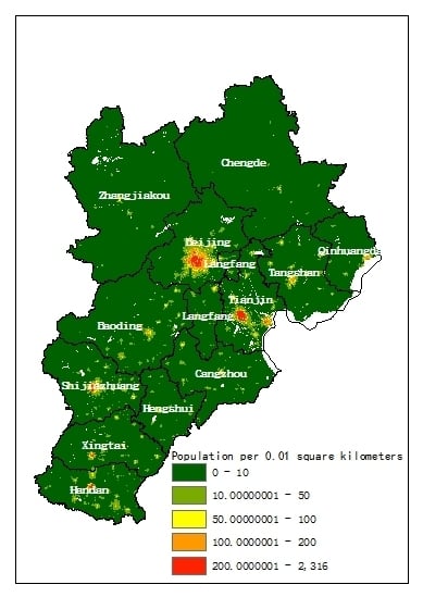
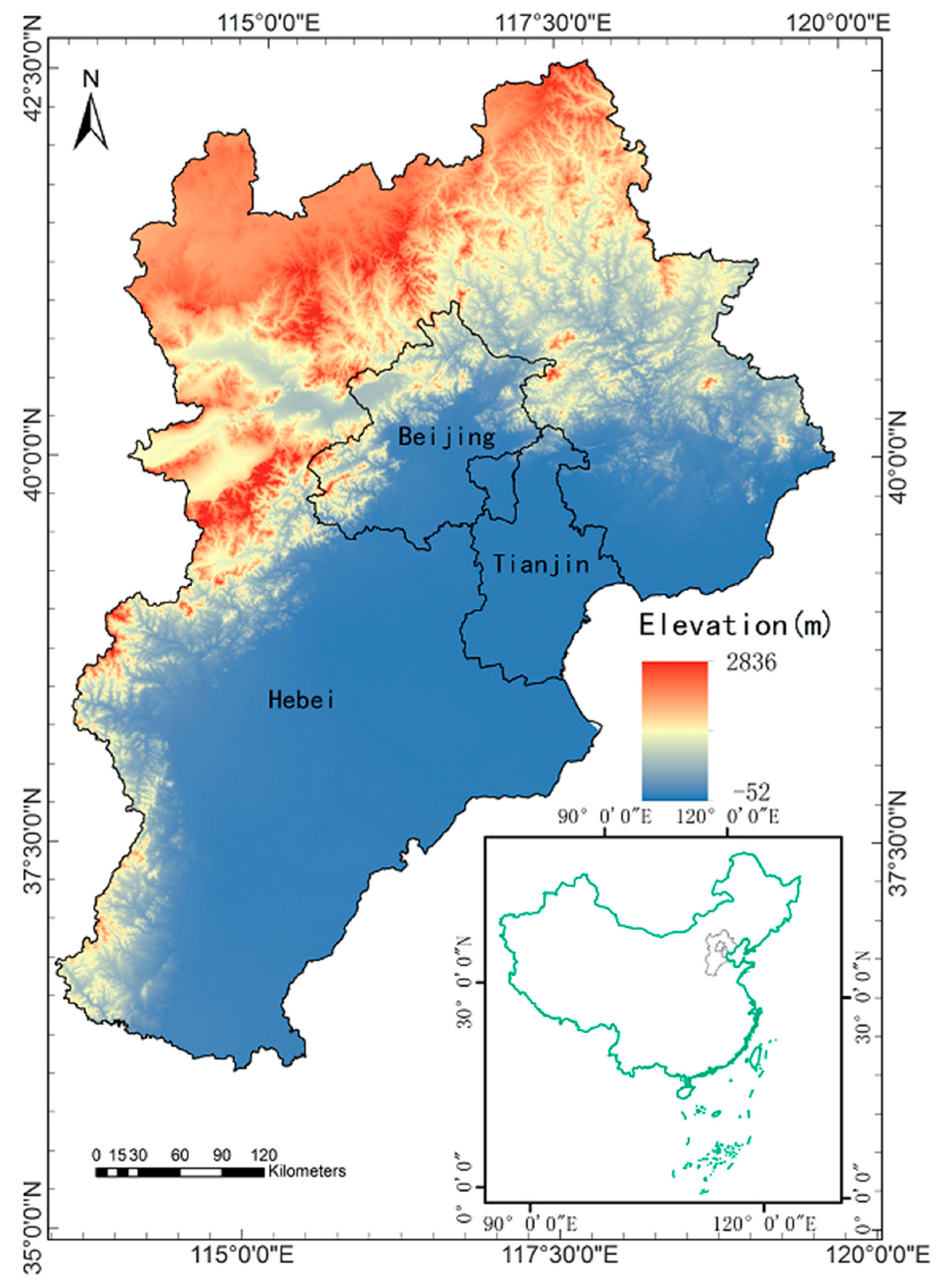
The Beijing-Tianjin-Hebei urban agglomeration consists of the municipalities of Beijing and Tianjin and Hebei province, which is located at 42°40’ N~36°03’ N, 113°27’ E~119°50’ E. It is the largest urbanized megalopolis region in northern China and the capital region of China. Figure 1 showed the elevation map of the experimental area, the overall topography of it shows high in the northwest and low in the southeast. The terrain and geomorphology of the BTH are heterogeneous, gradually transforming from grasslands to mountains and to plains from the northwest to southeast. The BTH is the "capital economic circle" of China and has the largest economy in northern China. The region covers an area of 218,000 square kilometers, including 2 municipalities and 11 prefecture-level cities. In 2016, the GDP of the BTH totaled 7461.26 billion RMB, accounting for 10% of the national total. The total population reached approximately 112.48 million in 2017, accounting for more than 8% of the national total. The BTH extends over areas with high (e.g., Beijing) and low population density (e.g., the Bashang Grasslands). This makes the BTH a suitable experimental area for exploring the influence of the population-sensitive POI types in the dasymetric mapping.
2.2. Data and Preprocessing
Remotely sensed products and geospatial big data (Table 1) were collected for the development of the dasymetric model and the generation of a fine-grained population map. All the input data were processed to raster layers with a consistent resolution of 100-m and used as covariates in the dasymetric model.
2.2.1. Demographic Data
The demographic data were obtained for Beijing, Tianjin and Hebei from the China Statistical Yearbook published by the National Bureau of Statistics of China. The demographic data were collected at two scales. The demographic data of all 204 counties in the BTH (16 in Beijing, 16 in Tianjin and 172 in Hebei) were used for the development of the dasymetric models. Finer-scale demographic data were further obtained for all 292 towns in Beijing. These data were used to evaluate the accuracy of the fine-grained population map and other datasets. These towns cover a variety of land cover types and consist of both urban and rural areas, with population densities ranging from 16 to 41,979 people per square kilometer. Therefore, it is believed that the accuracy estimated using these finer-scale demographic data in Beijing can represent the overall accuracy in the BTH.
2.2.2. Geospatial Big Data
POI data, the influence of which is to be explored in this study, are among the most important covariates in population dasymetric mapping. The POI data were retrieved from NavInfo, the leading provider of navigation maps, navigation software, dynamic traffic information, location big data, and customized vehicle networking solutions for passenger cars and commercial vehicles in China. The study included a total of 1,789,292 POI records in 15 categories of the BTH (Table 2). Moreover, two raster layers were produced for each POI category. Kernel density estimation (KDE) was applied to each category to generate a smooth and continuous POI density layer [34,47]. KDE is a well-known method to estimate the probability density function of a random variable. KDE uses a quadratic formula to disperse the surface around each point and output pixel with the cumulative value of every surface. In addition, the distance to the nearest POI was also calculated for each POI category.
The Easygo heat map is a high-resolution real-time population density map; it is produced by Tencent, one of the largest internet-based technology and cultural enterprises in China. The Easygo heat map data were used in combination with POI data in this study to identify the population-sensitive POIs. Each record in Easygo heat map contains three parts, longitude, latitude, and count, representing the location and number of users of the Tencent products, such as QQ, WeChat and Tencent Maps. The number of active Tencent users reached 9 billion in 2016, making the Easygo heat map a reliable data source to examine the overall population distribution. In this study, a web crawler was developed to acquire Easygo heat map data from May 6th to May 11th, 2019, at 20:00, 21:00 and 22:00 during after-work hours on workdays. The population density of these time periods was averaged to represent the permanent population distribution [35].
The road network, river network, and water body data were obtained from OpenStreetMap (OSM) (https://www.openstreetmap.org/). OSM is a collaborative project to create a free editable map of the world. The OSM data are crowdsourced and characterized by fast updates. The road network, river network, and waterbody data from OSM were obtained to generate the covariates for population mapping. Seven covariates were generated from the OSM data, including the road density, the length of different types of road networks (railway, motorway, primary way and secondary way), the distances to the waterbody and the density of the river networks.
2.2.3. Remotely Sensed Products
Many studies have found that night-time light data have strong associations with the population distribution [47,48]. Thus, night-time light data can be used as a basic covariate for generating a population map. The Visible Infrared Imaging Radiometer Suite (VIIRS) (https://ncc.nesdis.noaa.gov/VIIRS/) on board the Suomi National Polar-orbiting Partnership spacecraft could produce a suite of average radiance composite images using night-time light data from the VIIRS Day/Night Band (DNB). These data can identify weak light sources, which can be used in the study of the atmosphere, surface processes, and human activities. The VIIRS products have a spatial resolution of approximately 500 m and are produced on a monthly and annual basis. In this study, the VIIRS nighttime light composites were obtained and preprocessed to filter out lights from fires, boats, the aurora, and other temporal lights.
The land use and land cover data were obtained from the MODIS Land Cover Type Product (MCD12Q1) (https://lpdaac.usgs.gov/), which supplies global maps of land cover at annual time steps and 500-m spatial resolution from 2001 to present. The MCD12Q1 product was downloaded, and the International Geosphere-Biosphere Program (IGBP) classification scheme was adopted, classifying the land surface into 17 land cover types. The urban and built-up land cover class were extracted to generate the covariate of distance to built-up lands.
The Shuttle Radar Topography Mission (SRTM) digital elevation data (https://www2.jpl.nasa.gov/srtm/) were also collected to generate the covariates of elevation and slope. The resolution of the SRTM dataset is 1 arc second (approximately 30-m). Most parts of the world have been covered by this dataset, which ranges from 54°S to 60°N latitude, including Africa, Europe, North America, South America, Asia, and Australia.
2.2.4. Datasets for Accuracy Comparison
The two gridded population datasets, WorldPop (https://www.worldpop.org/) and LandScan (https://landscan.ornl.gov/), were acquired; their accuracy was then compared with that of the PSP-based population maps. The global per country datasets from WorldPop provide a 100-m resolution annual worldwide gridded population maps from 2000 to 2020. It is among the finest spatial resolution population maps produced for China. The LandScan dataset is a global gridded population dataset with a spatial resolution of approximately 1 km produced annually from 2000 to 2017. Both of these datasets were popular and have been widely used in monitoring population changes [49,50]. Both the WorldPop and LandScan data for 2017 were obtained to compare with the PSP-based population map.
3. Methods
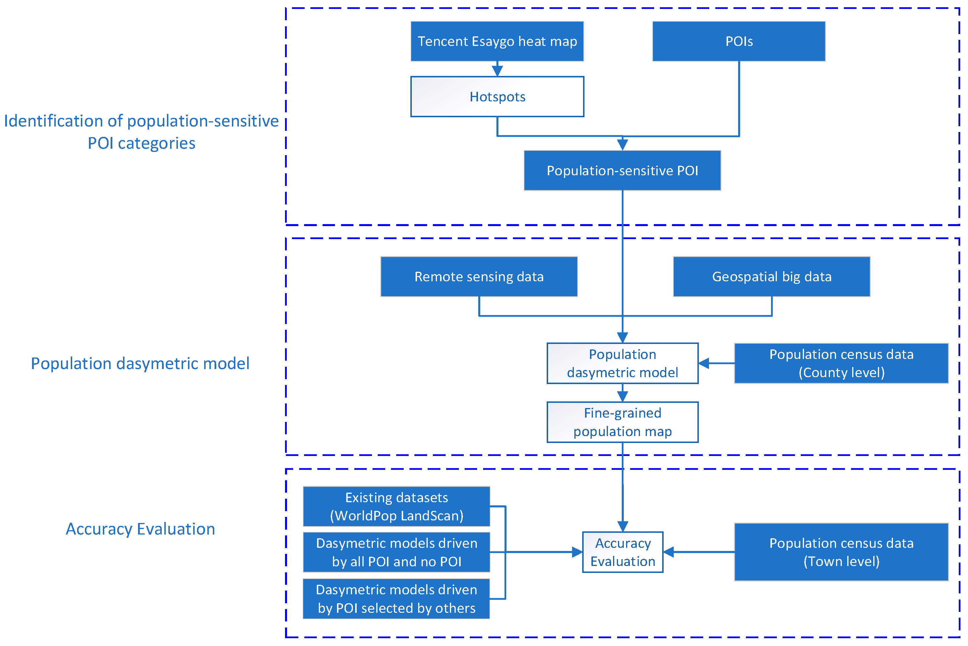
In this study, Easygo heat map data were used to extract the population hotspots and to identify population-sensitive POIs. The thereby identified PSPs were further fed into a random forest model to downscale the county-level population, together with population-related remotely sensed products and geospatial big data. Finally, the fine-grained population map resulting from the PSP-driven dasymetric model was compared with the WorldPop and LandScan datasets and the population map generated by dasymetric models with all POIs, no POIs, and POI categories selected by other studies. The accuracy of these datasets was evaluated using population census data at the subdistrict scale. The entire flowchart of the study is outlined in Figure 2 and described below.
3.1. Identification of Population-Sensitive POI Categories
Many studies have made large improvements that have considered introducing POIs to training population downscaling models; however, these models have trouble been hampered by ignoring the uncertainties of some categories of POIs in their models. This study aims to solve this problem by identifying the PSPs using spatial association mining. The PSPs were identified as the POIs that were spatially associated with population hotspots.
The population hotspots were extracted by applying the Anselin Local Moran’s I index on the permanent population distribution map derived from Tencent Easygo heat map. The Anselin Local Moran’s I index has been demonstrated to be an effective tool to identify hotspots, cold spots, and spatial outliers with statistical significance [51,52]. The Cluster and Outlier Analysis tool using default parameters from ArcMap 10.5 was used to calculate the Anselin Local Moran’s I value of each record of Tencent Easygo heat map data and identify the population hotspots in this study.
The PSP categories were then determined through spatial association rule mining. The spatial association rule represents the relationship between spatial features [53]. In this study, the distance metric was relied on to quantitatively describe the relationship between the population hotspots and POIs. To obtain all the spatial association rules between population hotspots and POI records, an adjacency table between POIs and each population hotspot was generated. Each adjacency table was treated as an item that was the basic unit of input data for an association rule mining algorithm. As an association rule mining algorithm, the FP-growth algorithm was used to find the strong association rules between population gathering points and POIs. The FP-growth algorithm is one of the most widely used association rule mining algorithms [54]. The idea of this algorithm is to construct a compressed data structure, the FP-tree, to store all the transaction items. Then, the association rules were achieved from FP-tree. An association rule can be shown as follows:
where X is the antecedent and Y is the consequent of the spatial association rules. The association rule is evaluated by two parameters of support and confidence [55] as follows:
where support is an importance measure of association rules, while confidence is an accuracy measure of association rules. The degree of support indicates how representative the rule is among all spatial objects. Strong association rules were identified as those with both high support and confidence. This guarantees that these rules are important and accurate.
3.2. Population-Sensitive POI Driven Dasymetric Model
The dasymetric model has been demonstrated to be effective in fine-grained gridded population mapping. In this study, a new dasymetric model was established to generate a fine-grained population map by introducing PSPs. The random forest (RF) model [56] was selected to construct the dasymetric model using the log-transformed population density as the response variable and the mean value of each covariate as the independent variables. The RF model is a nonparametric model that has been widely used in classification or regression problems by growing a “forest” of individual classification or a set of regression trees. The bootstrap sampling technique was used to select some of the samples randomly from the original training sample to generate a training decision tree and to repeat this process many times to form a forest. The results were determined by all the trees in the forest. Data not selected in the bootstrap process are called out-of-bag (OOB) data. According to previous studies [57,58,59], the OOB error estimation is an error estimation method that can replace that using the test set. Moreover, the RF model has the advantage of not having to filter features when processing multidimensional data, and having fewer adjustment parameters. These makes RF an ideal model for this study.
In this study, the response variable of the RF model was set as the log-transformed population density in each county or district to create more normal and evenly distributed density values with respect to the covariates [18]. Model estimation, fitting, and prediction were performed using the statistical environment R 3.5.2 [60] and the randomForest package [61]. The model has two adjusted parameters, mtry and ntree. The former parameter determines the number of randomly selected covariates for each tree, and the latter determines the number of trees in the forest. After many experimental training repetitions, we finally decided [60] that a 500 tree forest with 4 covariates for each tree could obtain a stable, minimized OOB error of prediction. This RF model was finally applied to the raster layers of the covariates to predict the log population densities for each pixel. The per-pixel raster was used as a weight layer, according to which the population of a county could be distributed to each pixel.
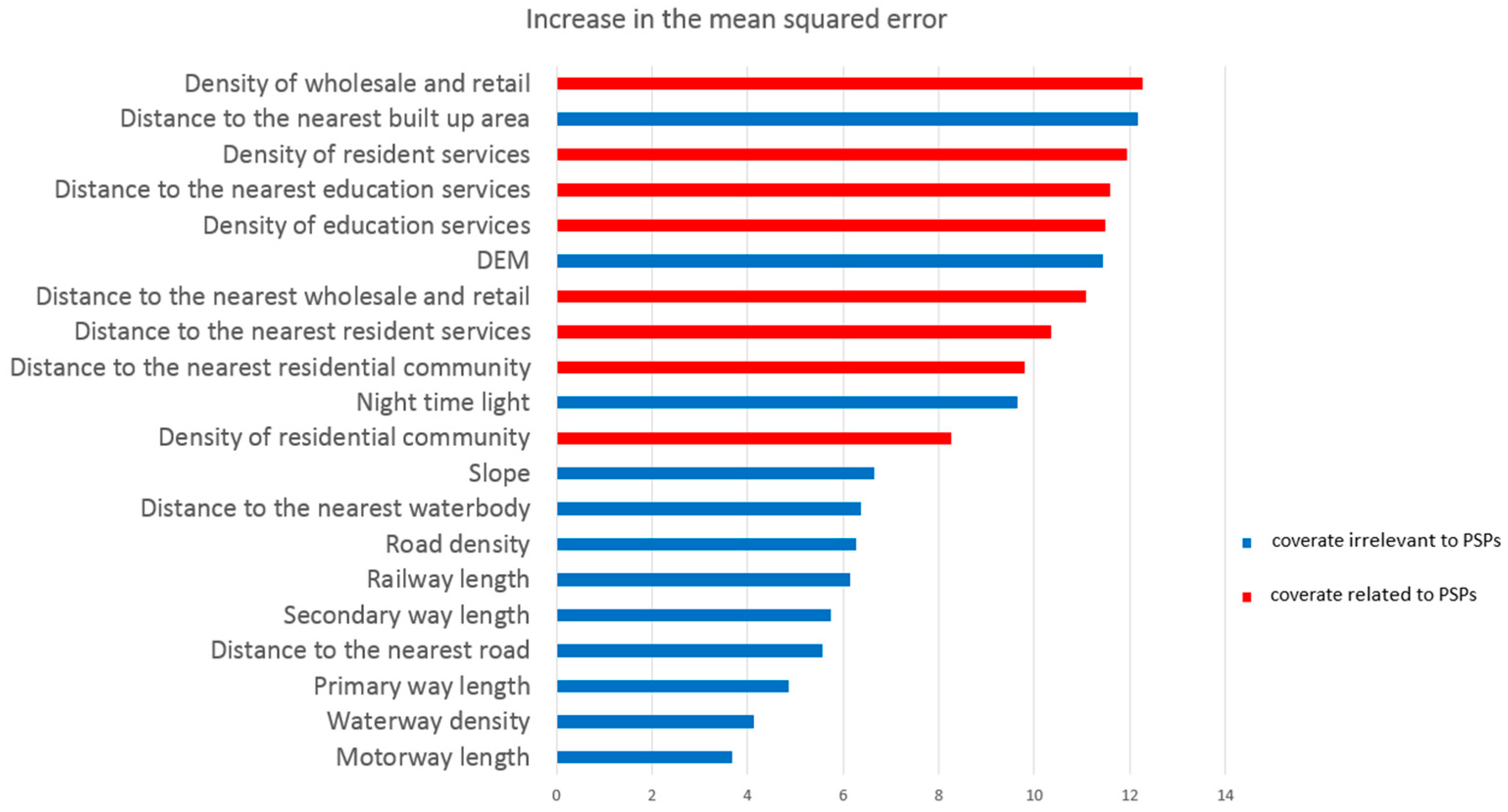
The importance of each covariate can be evaluated in R based on the increase in the mean squared error (%IncMSE). %IncMSE represents the increase in MSE with a change in the covariate. The importance of the variable for the RF regression was presented as the mean decrease in the residual sum of squares when the tree containing this variable was split [18], so %IncMSE could express the importance of variables. %IncMSE is based on the OOB error, which represents the change in error after modification; the larger %IncMSE is, the more important the value.
The pixel level map calculated by the RF model above is not the actual population distribution map; it is just the weighting layer for the log-transformed population density. There are a few additional steps required to obtain the final population distribution map. The first step is to back-transform the log and obtain the population density for each pixel. Next, pixels in areas with no population distribution, such as water bodies, need to be assigned a value of zero. Finally, the per-pixel population density calculated by the RF model is the estimate of population density and covariate values in every administrative unit; therefore, the actual population density distribution needs to control the total population of each county using the following equation:
where is the population in grid , is the population of the county where grid is located, is the weight associated with grid as predicted by the random forests model, and is the sum of weights of all pixels within county .
3.3. Accuracy Assessment and Comparison with Other Population Datasets
The fine-grained population map produced in this study was based on the county-level demographic data. A finer-level population demographic dataset was needed to evaluate its accuracy. In this study, the demographic data of all 292 towns in Beijing were used for this purpose by validating the sum of the predicted population of all grids within a town against the population of that town reported in the yearbook. All towns were divided into three categories according to their population densities. The towns with the largest 30% of the population densities were defined as high population density areas, those with the smallest 30% of the population densities were defined as low population density areas, and the remaining towns were defined as medium population density areas. Among these, 88 towns were classified as high population density areas (more than 10,896 people per kilometer), 116 towns were classified as medium population density areas (more than 473 people per square kilometer and less than 10,896 people per square kilometer) and 88 towns were classified as low population density areas (less than 473 people per square kilometer). To evaluate the accuracy of the PSP-driven dasymetric model, three sets of comparative experiments were designed. First, the results of this study were compared with the WorldPop 2017 and LandScan 2017 datasets. Second, the results were compared with population maps generated by the dasymetric models driven by all POI records and no POI records. Finally, the results were compared with the population maps generated by the dasymetric model driven by the POI categories selected in other studies that did not consider the spatial association between the POIs and population. The accuracy of these data was evaluated by three measurements, namely, mean absolute error (MAE), root mean square error (RSME), and relative root mean square error (%RMSE) as follows:
where represents the estimated population value of town i, is the reference population of town i obtained from demographic data, and N represents the number of towns.
4. Results and Analysis
4.1. Population-Sensitive POI Categories
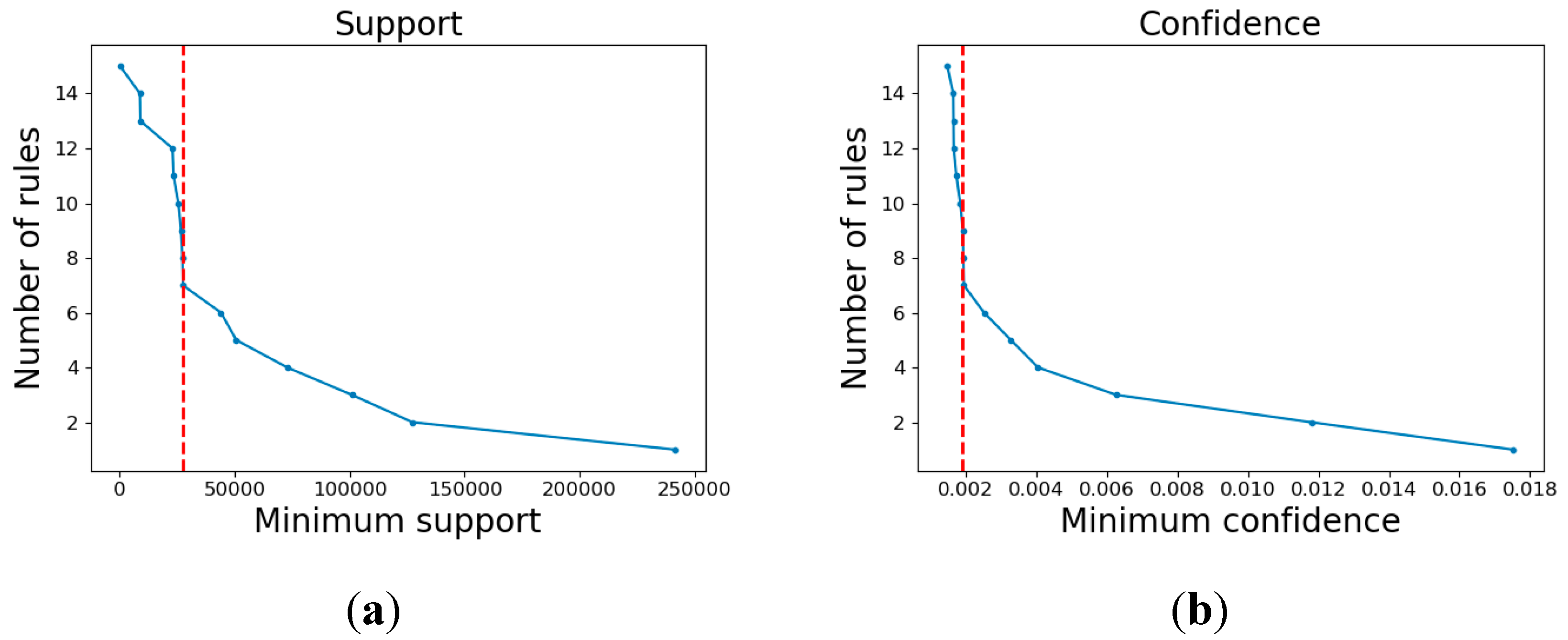
The PSP categories were selected by spatial association rule mining (see Section 3.1), which has a strong spatial association with the population hotspots extracted from Easygo heat map data. The two parameters of the spatial association rules between the POI categories and the population hotspots are shown in Table 3. Various categories had significant differences in the support and confidence of the association rule between the population hotspots and the POI categories. A total of 3092 hotspots were extracted to establish the two-dimensional association rules between population hotspots and POI records. The minimum support (min_sup) and minimum confidence (min_conf) values were determined to analyze the relationship between the number of association rules and different min_sup and min_conf values.
The number of association rules corresponding to the different min_sup and min_conf values showed obvious regularity (Figure 3). With increasing min_sup and min_conf values, the number of rules decreased. By analyzing the support values and confidence values, it was that some association rules contained certain categories of POIs, such as catering and corporation, that had high support but low confidence. This was because many of those POIs had a low proportion of spatial association rules with population aggregation points, which means that those association rules were important but not accurate. Other rules, such as the rules containing financial services and scientific research and technical services, had high confident and low support. Those categories of POIs were more likely to have association rules with population gathering points, but the number was small, which means that those association rules were accurate but not important. To obtain sufficient association rules that were important and improve the accuracy, the values of min_sup and min_conf should be set to be as large as possible and to obtain as many rules as possible at the same time. In this study, the value of min_sup was set to 27,450 and the value of min_conf was set to 0.0019, which is the abscissa of inflection points of Figure 3a,b. Finally, four categories were selected as PSPs, including residential community, wholesale and retail, education services, and resident services. The PSPs accounted for only 52% of the total POI records. This means that the other 48% were PIPs that would have inevitably introduced noise into the dasymetric model if all POIs were used.
The residential community contained POIs representing residential buildings, apartments, and hotels, where people lived and gathered. Wholesale and retail, education service, and resident service were the three categories of POI that were most relevant to people’s daily life, and they were also the attraction factors for residents. Therefore, all the PSP categories selected through the spatial association rule mining were closely related to the spatial distribution of the population and can be used in dasymetric mapping.
4.2. Population Map from the PSP-Driven Model
A RF-based dasymetric model was built with all the covariates described in Section 3.2. This model was used to downscale the log-transformed population density in each county. The fine-grained population map was built by back-transforming the result of the dasymetric model.
Figure 4 shows the value of %IncMSE for each covariate in the RF model. The importance of covariates to the PSPs was significantly higher than those of most other the covariates, which shows that PSP had a great impact on the accuracy of the dasymetric mapping. In addition to the covariates related to the PSPs, the distance to the nearest build-up area, DEM and NTL also has a large impact on the dasymetric modelling. This result is consistent with those of previous studies [16,18,47].
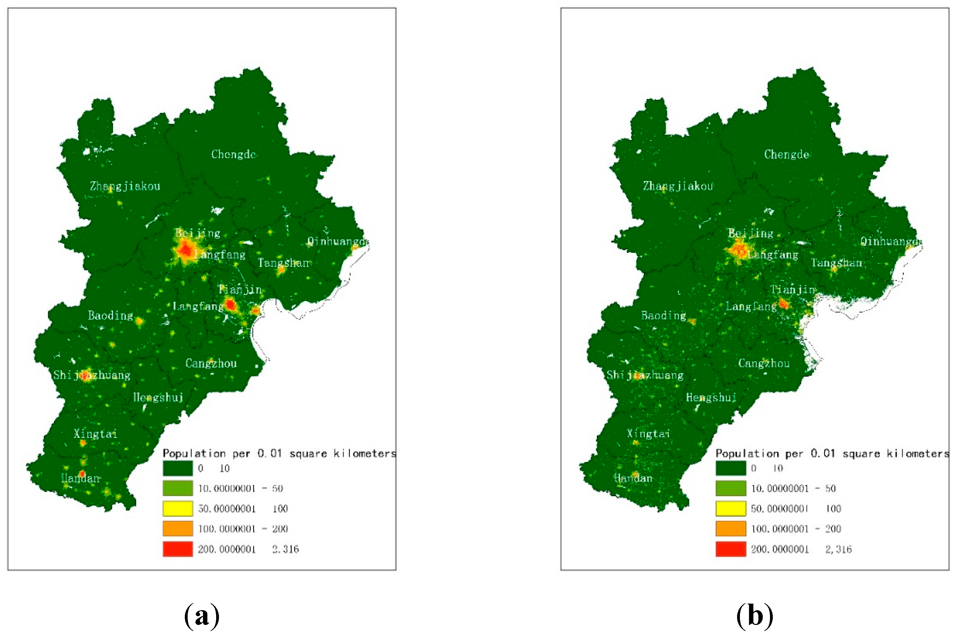
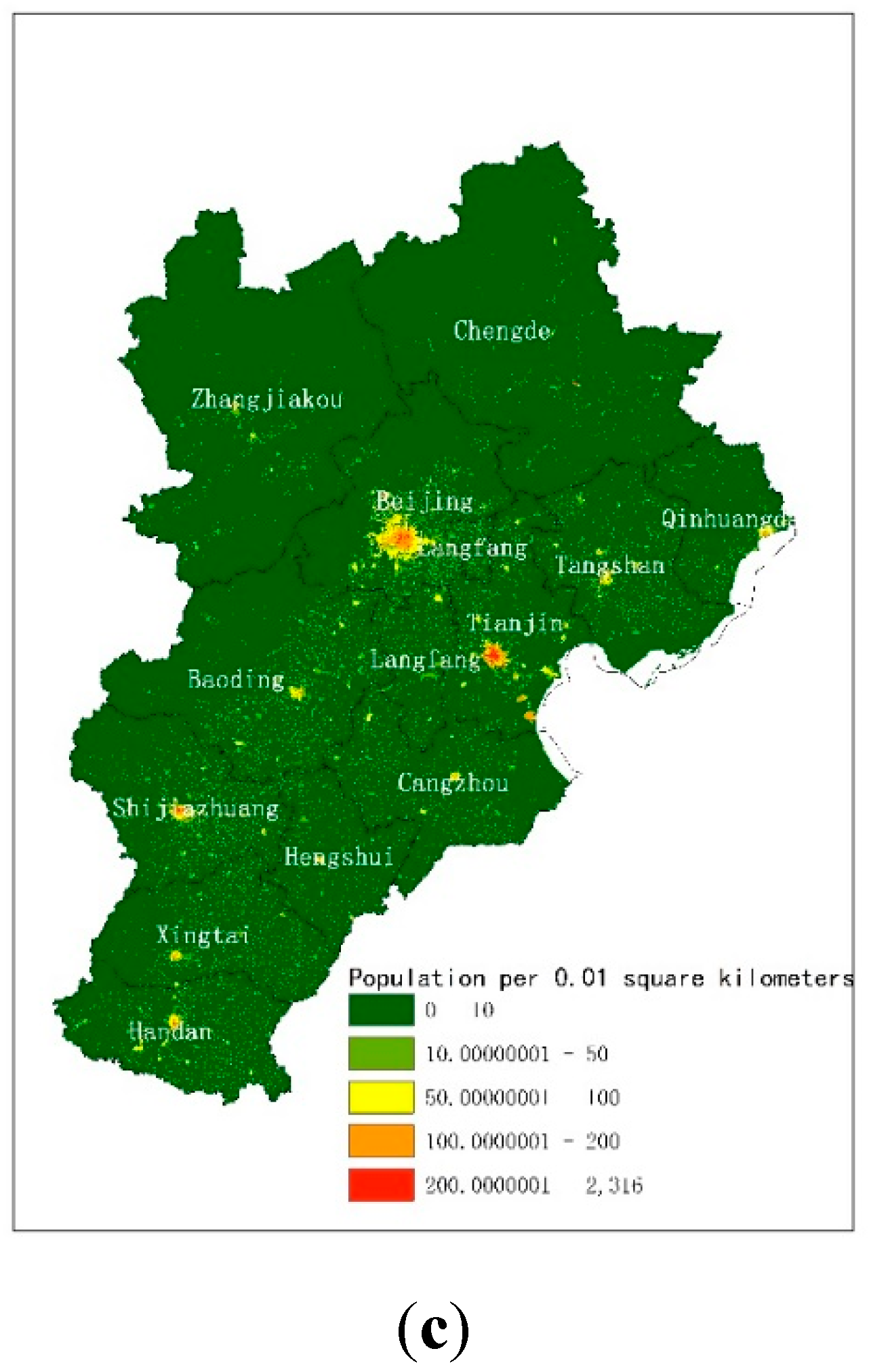
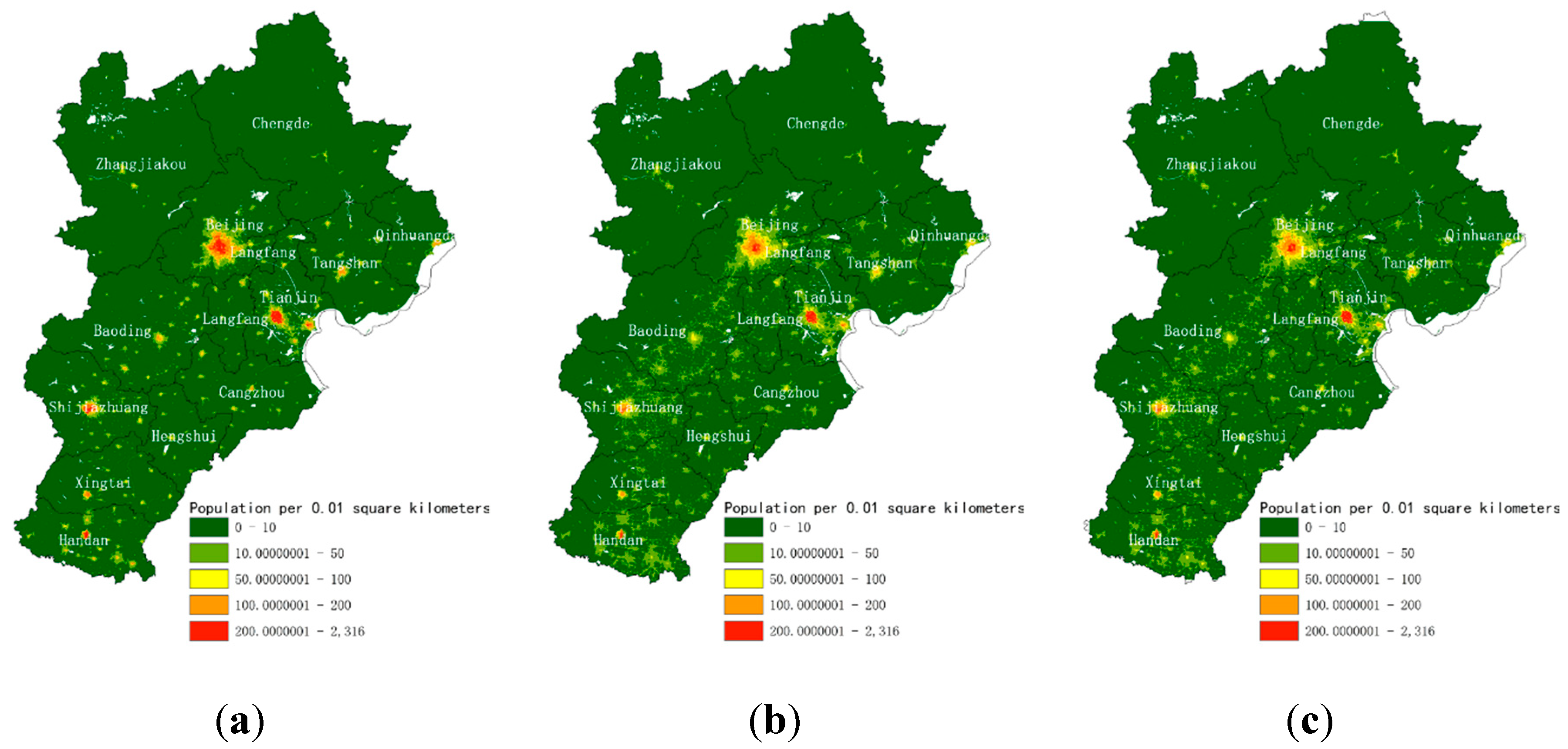
The fine-gridded population map at a 100-m spatial scale in the experiment showed visually satisfactory results (Figure 5). Figure 5a shows the population distribution map generated by the PSP-driven dasymetric model proposed in Section 3.2. As a comparison, the WorldPop (Figure 5b) and the LandScan (Figure 5c) datasets from the same region were also shown. Generally, the distributions of the population from three datasets were similar and agreed with the actual topography. The population of the plains and urban areas in the southeast was significantly higher than those in the mountains and grasslands in the northwest. The population was concentrated in the two municipalities of Beijing and Tianjin and aggregated in second-tier cities such as Shijiazhuang and Tangshan, which is consistent with the actual population distribution. Nevertheless, the results from the proposed methods also highlight the population gradient around small towns and villages.
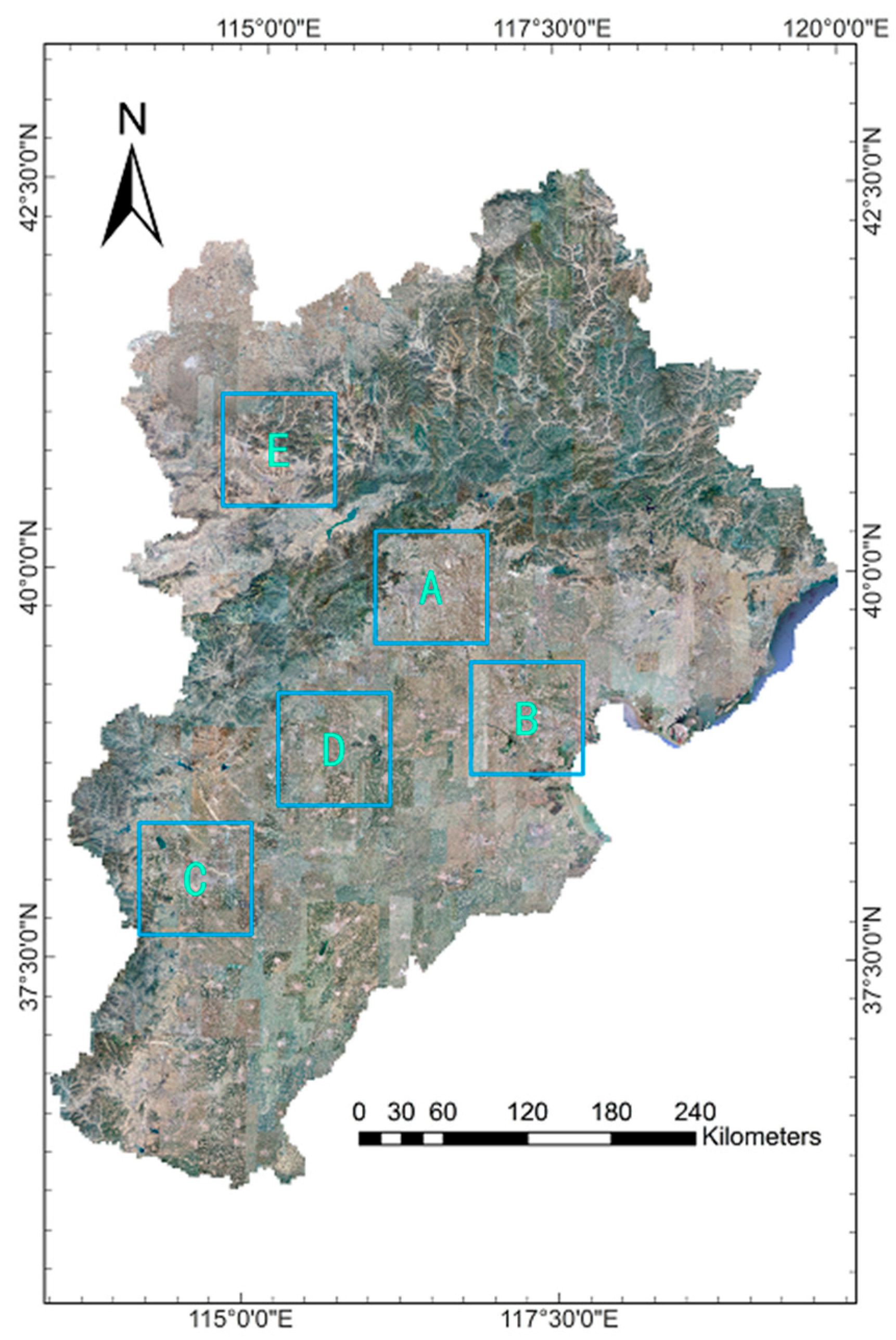
To further illustrate the effects of the population distribution map in this study, five regions were selected for a comparison of the results of the study with the other two datasets. Five different regions with different population densities were selected for further analysis (Figure 6). Beijing, as the capital city of China and one of the most populous cities in China (A), represented the region with the highest population density in our experimental area. Tianjin (B) was also selected to represent regions with high population density because the population reached 15.6 million at the end of 2017. Shijiazhuang (C) and Baoding (D), as the two most populous cities in Hebei province, were selected because of their high population density in urban areas and medium population density in the areas surrounding Shijiazhuang and Baoding. Zhangjiakou (E) was selected to represent a region with low population density located in the northwest of Hebei province (the southern edge of Inner Mongolia plateau with an altitude of 1300–1600 m).
The population distribution maps proposed in this study more closely reflected the real distribution than the other two datasets in all five regions. The high-resolution gridded population map of the study presented high spatial heterogeneity and few boundary effects, which could reflect the abundant population distribution information. According to the visual analysis of Figure 7a,b, the results of the PSP-driven dasymetric model reflected not only the concentration of the population in the city areas but also more details of the population distribution within the city, such as the distribution of different types of roads. Moreover, the population map from this study showed a weak boundary effect, and the population changes at the urban boundaries were smooth and natural. In Figure 7c,d, the results from this study reflected not only the population aggregation of various towns and villages but also the differences in the population densities of villages of different sizes. The northeast area in Figure 7e is located in a highland area with a low population density. Compared with the other two datasets, the result of PSP-driven dasymetric model showed that there was a smaller population in this area than the other two datasets. The difference between these datasets indicated that with the assistance of PSPs, the dasymetric mapping could weaken the direct impact of the DEM.
4.3. Accuracy Assessment
The fine-grained population map produced by the PSP-driven dasymetric model was produced based on the county-level demographic data. To evaluate the accuracy of these data, a finer level of demographic data (town level) was used. The accuracy assessment used the following steps. First, the administrative boundary data were used to statistically analyze the populations estimated by different population maps in each town and compared with the demographic data. Second, all the towns were divided into three groups according to population densities. Finally, the accuracy of the overall area and the three groups of towns was assessed using three measurements: MAE, RMSE, and %RMSE.
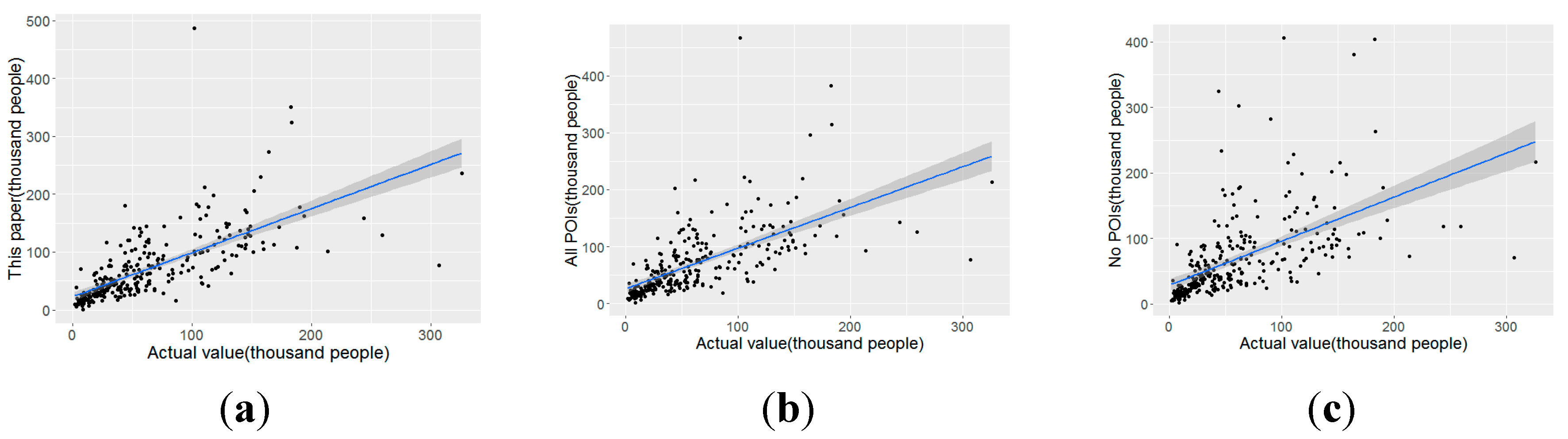
Table 4, Figure 8 and Figure 9 show the results of the population maps generated by the dasymetric model driven by PSP records, all POI records, and no POI records. The population map produced by the PSP-driven dasymetric model had the highest accuracy not only in all areas but also for each category. The accuracy of the model with all POI records was higher than that of the model with no POI record in most areas except for areas with low population densities. The reason for this phenomenon may be that population-insensitive POI categories are not associated with the population distribution, and introducing these data would interfere with dasymetric mapping.
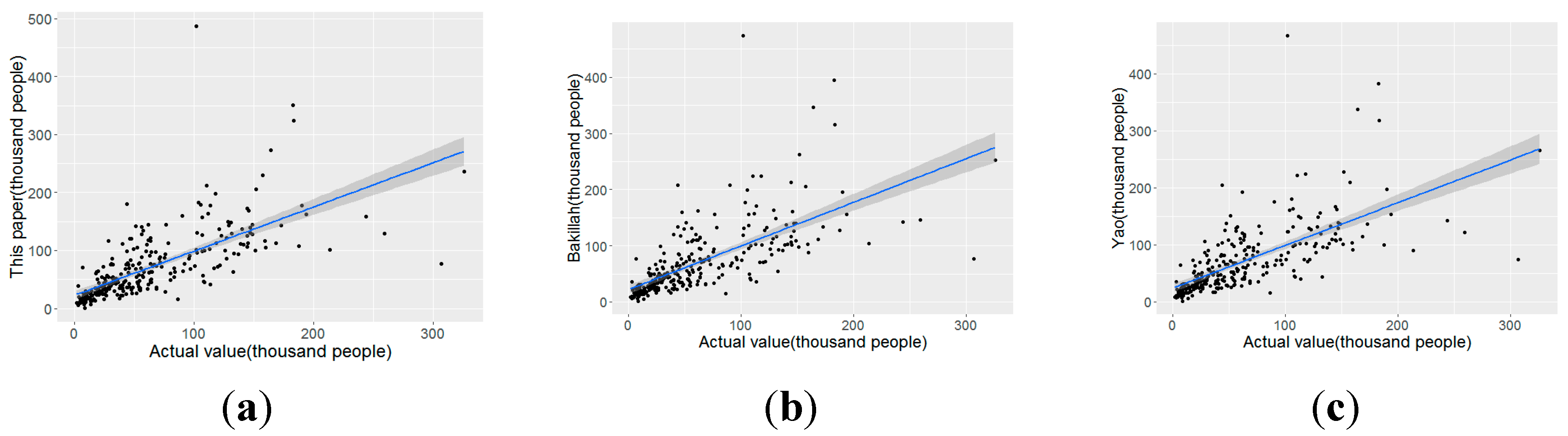
The PSP categories in this study were selected by spatial association rule mining between POI records and population gathering points. To our knowledge, all previous studies have used POIs separately and have only considered the quantitative relationship between the POIs and population. To compare the impact of the POI categories selected by different methods on dasymetric modelling, the models were built with different POI categories. The PSP categories selected in this study were residential community, wholesale and retail, education services, and resident services. Reference data were obtained from the studies of Bakillah [1] and Yao [3]. Bakillah used Spearman’s correlation coefficient to calculate the correlation between the occurrences of a category of POI and the population density in administrative blocks and found that the “high-density indicator” (HDI) POI categories were education services and transportation and storage. Yao used term frequency-inverse document frequency (TF-IDF) to filter the meaningless high-frequency POIs, such as the name tags of roads and districts, determined that the HDI POI categories were medical institution, residential community, and education services. Figure 10 shows the different population map generated by dasymetric model driven by different categories POIs. Table 5 and Figure 11 shows that the accuracy of the PSP-driven dasymetric model was higher than those of the models driven by the HDI POIs selected by Bakillah and Yao in almost every area, except in low population density areas, where the accuracy was slightly lower than that of the model driven by the HDI POIs selected by Bakillah. By comparing the results from the models with no POI records, it is evident that both sets of HDI POI categories can improve the accuracy of dasymetric mapping, but not as much as the accuracy can be improved by the PSP categories.
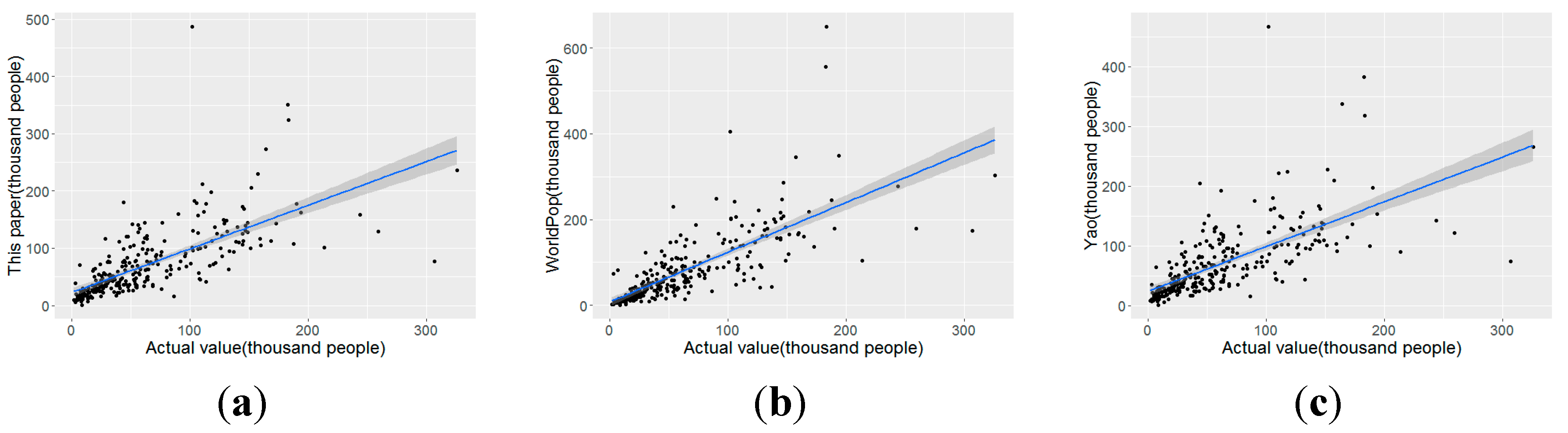
Table 6 and Figure 12 show the accuracy assessment results of this study and the WorldPop and LandScan datasets. Overall, the accuracy of the fine-grained population map generated in this study was significantly higher than those of the WorldPop and LandScan maps, especially in areas with high and medium population densities. However, the accuracy of the population map was slightly lower than those of the other two datasets. According to these data, we find that the accuracy of the PSP-driven dasymetric model increases with increasing population density. The reason may be as follows. The numbers of categories and quantities of POIs in low population density areas are lower than those in other areas, which meant that the covariates of this model were not sufficiently accurate. The statistics of the POIs in areas with low population densities are incomplete, and many new POIs may not be marked. The population attractiveness of the POIs in areas with low population density may differ from those in areas with high population density.
5. Conclusions and Discussion
With the rapid development of society and the acceleration of population flow, the traditional population maps cannot meet the needs of urban planning, disaster prevention, and environmental protection. In this case, an accurate population map is essential. Dasymetric mapping has been widely used to downscale demographic data in recent decades, and the accuracy of dasymetric mapping depends on the selection of covariates. As the product of the development of network information technology and mobile positioning technology, POIs have become important covariates in dasymetric mapping. However, the use of POIs to downscale demographic data is associated with certain problems arising from the indiscriminate use of POI records. This study innovatively used spatial association rule mining to identify PSPs and achieved improved population mapping accuracy using the PSP-driven dasymetric model. The accuracy of the fine-grained population map that used the proposed model in this study was more accurate than those of the WorldPop and LandScan maps for population estimation, especially in high-density regions. By comparing the accuracy of the dasymetric models driven by different POI categories, the following conclusions can be drawn by this study.
POI records, especially PSPs, can improve the accuracy of dasymetric mapping. The improved accuracy from by using PSPs in dasymetric mapping was verified by the comparison of the two dasymetric models driven by all POI records and no POI records. Although the dasymetric model driven by all POI records could also improve the accuracy of population estimation, it did not improve the accuracy as much as the PSP-driven dasymetric model. Therefore, it can be concluded that PSPs have a strong spatial association with the population distribution and can improve the accuracy of the population estimation in dasymetric mapping.
Spatial association rule mining can effectively identify PSP categories. The two groups of POIs obtained by other scholars through quantitative relationship screening were modelled separately, and the accuracy of those models was compared with that of the model proposed in this study. The accuracy of the PSP-driven dasymetric model was higher than those of the other two models. Based on these comparisons, a conclusion can be drawn that the PSP categories selected in this study have a more positive effect on population estimation because the spatial collocation between the POIs and population distribution was considered.
However, there are still limitations of using POIs to reflect the population distribution. As shown before, the accuracy of population map generated by PSP driven dasymetric model is less accurate in areas with low population density. The main reason of this phenomenon is the quality of POI records in these areas is instability [1]. The renewal speed and completeness of the POIs in rural areas are not as good as those in urban areas. This makes the quality of POIs unstable. Mocnick gives four measures to assess the data quality [62]. We use the data-based grounding measure by comparing POIs we used with Baidu Map and found that the data quality of POIs in rural area is lower than urban area. Another reason is that POIs in different population density areas may have different abilities to attract population. We found that the population size of the low population area is often overestimated in models using POI data, this may be because POIs in these areas are less attractive to the population than other regions. To further improve the accuracy of the low population density area, different population areas can be modeled separately to change the weight of POI-related variables in different areas. Moreover, we only found the two-dimensional association rules between population hotspots and different types of POIs, and the population distribution may have been influenced by multiple POI categories. With the continuous expansion of cities, the social life of human beings will be more abundant, and the POI categories of will be further refined and increased. In future research, the combined effects of multiple types of POIs on population distribution will be considered to further improve the accuracy of the population distribution estimations.
The results of this study may provide ideas or be a reference for many other studies. Since POIs can be used in analyzing the population distribution, many other distribution patterns of information associated with the population could also be analyzed, such as age, gender, income level, and purchasing power. By analyzing the distribution of PSPs, housing prices could be analyzed and reference can be provided for residential site selection. For city managers, PSPs can help to divide the urban functional area and to analyze regional development.
Author Contributions
Conceptualization, Y.Z. (Yuncong Zhao), Q.L. and Y.Z. (Yuan Zhang); methodology, Y.Z. (Yuncong Zhao); software, Y.Z. (Yuncong Zhao); data curation, Y.Z. (Yuncong Zhao); writing—original draft preparation, Y.Z. (Yuncong Zhao); writing—review and editing, Y.Z. (Yuncong Zhao), Q.L., Y.Z. (Yuan Zhang), and X.D.; supervision, Q.L.
Funding
This research was funded by Strategic Priority Research Program of Chinese Academy of Sciences, grant number XDA 20030302.
Acknowledgments
Great thanks to the anonymous reviewers whose comments and suggestions significantly improved the manuscript.
Conflicts of Interest
The authors declare no conflict of interest.
References
- Bakillah, M.; Liang, S.; Mobasheri, A.; Arsanjani, J.J.; Zipf, A. Fine-resolution population mapping using OpenStreetMap points-of-interest. Int. J. Geogr. Inf. Sci. 2014, 28, 1940–1963. [Google Scholar] [CrossRef]
- Jia, P.; Qiu, Y.; Gaughan, A.E. A fine-scale spatial population distribution on the high-resolution gridded population surface and application in Alachua County, Florida. Appl. Geogr. 2014, 50, 99–107. [Google Scholar] [CrossRef]
- Yao, Y.; Liu, X.; Li, X.; Zhang, J.; Zhaotang, L.; Mai, K.; Zhang, Y. Mapping fine-scale population distributions at the building level by integrating multisource geospatial big data. Int. J. Geogr. Inf. Sci. 2017, 31, 1220–1244. [Google Scholar] [CrossRef]
- Ahola, T.; Virrantaus, K.; Krisp, J.M.; Hunter, G.J. A spatio-temporal population model to support risk assessment and damage analysis for decision-making. Int. J. Geogr. Inf. Sci. 2007, 21, 935–953. [Google Scholar] [CrossRef]
- Dobson, J.E.; Bright, E.A.; Coleman, P.R.; Durfee, R.C.; Worley, B.A. LandScan: A global population database for estimating populations at risk. Photogramm. Eng. Remote Sens. 2000, 66, 849–857. [Google Scholar]
- Zeng, J.; Zhu, Z.Y.; Zhang, J.L.; Ouyang, T.P.; Qiu, S.F.; Zou, Y.; Zeng, T. Social vulnerability assessment of natural hazards on county-scale using high spatial resolution satellite imagery: A case study in the Luogang district of Guangzhou, South China. Environ. Earth Sci. 2012, 65, 173–182. [Google Scholar] [CrossRef]
- Aubrecht, C.; Ozceylan, D.; Steinnocher, K.; Freire, S. Multi-level geospatial modeling of human exposure patterns and vulnerability indicators. Nat. Hazards 2013, 68, 147–163. [Google Scholar] [CrossRef]
- Cutter, S.L.; Boruff, B.J.; Shirley, W.L. Social vulnerability to environmental hazards. Soc. Sci. Q. 2003, 84, 242–261. [Google Scholar] [CrossRef]
- Hay, S.I.; Noor, A.M.; Nelson, A.; Tatem, A.J. The accuracy of human population maps for public health application. Trop. Med. Int. Health 2005, 10, 1073–1086. [Google Scholar] [CrossRef]
- Jia, P.; Sankoh, O.; Tatem, A.J. Mapping the environmental and socioeconomic coverage of the INDEPTH international health and demographic surveillance system network. Health Place 2015, 36, 88–96. [Google Scholar] [CrossRef] [Green Version]
- Holt, J.B.; Lo, C.; Hodler, T.W. Dasymetric estimation of population density and areal interpolation of census data. Cartogr. Geogr. Inf. Sci. 2004, 31, 103–121. [Google Scholar] [CrossRef]
- Langford, M. Rapid facilitation of dasymetric-based population interpolation by means of raster pixel maps. Comput. Environ. Urban Syst. 2007, 31, 19–32. [Google Scholar] [CrossRef]
- Reibel, M.; Agrawal, A. Areal interpolation of population counts using pre-classified land cover data. Popul. Res. Policy Rev. 2007, 26, 619–633. [Google Scholar] [CrossRef]
- Lo, C. Population estimation using geographically weighted regression. GISci. Remote Sens. 2008, 45, 131–148. [Google Scholar] [CrossRef]
- Tobler, W.; Deichmann, U.; Gottsegen, J.; Maloy, K. World population in a grid of spherical quadrilaterals. Int. J. Popul. Geogr. 1997, 3, 203–225. [Google Scholar] [CrossRef]
- Wang, L.; Wang, S.; Zhou, Y.; Liu, W.; Hou, Y.; Zhu, J.; Wang, F. Mapping population density in China between 1990 and 2010 using remote sensing. Remote Sens. Environ. 2018, 210, 269–281. [Google Scholar] [CrossRef]
- Sorichetta, A.; Hornby, G.M.; Stevens, F.R.; Gaughan, A.E.; Linard, C.; Tatem, A.J. High-resolution gridded population datasets for Latin America and the Caribbean in 2010, 2015, and 2020. Sci. Data 2015, 2, 150045. [Google Scholar] [CrossRef] [Green Version]
- Stevens, F.R.; Gaughan, A.E.; Linard, C.; Tatem, A.J. Disaggregating census data for population mapping using random forests with remotely-sensed and ancillary data. PLoS ONE 2015, 10, e0107042. [Google Scholar] [CrossRef]
- Wardrop, N.A.; Jochem, W.C.; Bird, T.J.; Chamberlain, H.R.; Clarke, D.; Kerr, D.; Bengtsson, L.; Juran, S.; Seaman, V.; Tatem, A.J. Spatially disaggregated population estimates in the absence of national population and housing census data. Proc. Natl. Acad. Sci. USA 2018, 115, 3529–3537. [Google Scholar] [CrossRef] [Green Version]
- Balk, D.; Yetman, G. The Global Distribution of Population: Evaluating the Gains in Resolution Refinement; Center for International Earth Science Information Network (CIESIN), Columbia University: New York, NY, USA, 2004. [Google Scholar]
- Tobler, W.; Uwe, D.; Jone, G.; Kelly, M. The Global Demography Project (95-6); National Center for Geographic Information and Analysis Department of Geography: Santa Barbara, CA, USA, 1995. [Google Scholar]
- Eicher, C.L.; Brewer, C.A. Dasymetric mapping and areal interpolation: Implementation and evaluation. Cartogr. Geogr. Inf. Sci. 2001, 28, 125–138. [Google Scholar] [CrossRef]
- Mennis, J. Generating surface models of population using dasymetric mapping. Prof. Geogr. 2003, 55, 31–42. [Google Scholar]
- Mennis, J. Dasymetric mapping for estimating population in small areas. Geogr. Compass 2009, 3, 727–745. [Google Scholar] [CrossRef]
- Mennis, J.; Hultgren, T. Intelligent dasymetric mapping and its application to areal interpolation. Cartogr. Geogr. Inf. Sci. 2006, 33, 179–194. [Google Scholar] [CrossRef]
- Mrozinski, R.D.; Cromley, R.G. Singly-and doubly-constrained methods of areal interpolation for vector-based GIS. Trans. GIS 1999, 3, 285–301. [Google Scholar] [CrossRef]
- Nagle, N.N.; Buttenfield, B.P.; Leyk, S.; Spielman, S. Dasymetric modeling and uncertainty. Ann. Assoc. Am. Geogr. 2014, 104, 80–95. [Google Scholar] [CrossRef]
- Azar, D.; Engstrom, R.; Graesser, J.; Comenetz, J. Generation of fine-scale population layers using multi-resolution satellite imagery and geospatial data. Remote Sens. Environ. 2013, 130, 219–232. [Google Scholar] [CrossRef]
- Cai, J.; Huang, B.; Song, Y. Using multi-source geospatial big data to identify the structure of polycentric cities. Remote Sens. Environ. 2017, 202, 210–221. [Google Scholar] [CrossRef]
- Deville, P.; Linard, C.; Martin, S.; Gillbert, M.; Stevens, F.; Gaughan, A.; Blondel, V.; Tatem, A. Dynamic population mapping using mobile phone data. Proc. Natl. Acad. Sci. USA 2014, 111, 15888–15893. [Google Scholar] [CrossRef] [Green Version]
- Li, K.; Chen, Y.; Li, Y. The Random Forest-Based Method of Fine-Resolution Population Spatialization by Using the International Space Station Nighttime Photography and Social Sensing Data. Remote Sens. 2018, 10, 1650. [Google Scholar] [CrossRef]
- Li, X.; Zhou, W. Dasymetric mapping of urban population in China based on radiance corrected DMSP-OLS nighttime light and land cover data. Sci. Total Environ. 2018, 643, 1248–1256. [Google Scholar] [CrossRef]
- Yang, X.; Huang, Y.; Dong, P.; Jiang, D.; Liu, H. An Updating System for the Gridded Population Database of China Based on Remote Sensing, GIS and Spatial Database Technologies. Sensors 2009, 9, 1128–1140. [Google Scholar] [CrossRef] [PubMed] [Green Version]
- Yang, X.; Ye, T.; Zhao, N.; Chen, Q.; Yue, W.; Qi, J.; Zeng, B.; Jia, P. Population Mapping with Multisensor Remote Sensing Images and Point-Of-Interest Data. Remote Sens. 2019, 11, 574. [Google Scholar] [CrossRef]
- Zhang, Y.; Li, Q.; Wang, H.; Du, X.; Huang, H. Community scale livability evaluation integrating remote sensing, surface observation and geospatial big data. Int. J. Appl. Earth Obs. Geoinform. 2019, 80, 173–186. [Google Scholar] [CrossRef]
- Canavosio-Zuzelski, R.; Agouris, P.; Doucette, P. A photogrammetric approach for assessing positional accuracy of OpenStreetMap© roads. ISPRS Int. J. Geo-Inf. 2013, 2, 276–301. [Google Scholar] [CrossRef]
- Touya, G.; Antoniou, V.; Olteanu-Raimond, A.; Damme, M. Assessing crowdsourced POI quality: Combining methods based on reference data, history, and spatial relations. ISPRS Int. J. Geo-Inf. 2017, 6, 80. [Google Scholar] [CrossRef]
- Gao, S.; Janowicz, K.; Couclelis, H. Extracting urban functional regions from points of interest and human activities on location-based social networks. Trans. GIS 2017, 21, 446–467. [Google Scholar] [CrossRef]
- Hu, T.; Yang, J.; Li, X.; Gong, P. Mapping urban land use by using landsat images and open social data. Remote Sens. 2016, 8, 151. [Google Scholar] [CrossRef]
- Jiang, S.; Alves, A.; Rodrigues, F.; Ferreira, J.; Pereira, F. Mining point-of-interest data from social networks for urban land use classification and disaggregation. Comput. Environ. Urban Syst. 2015, 53, 36–46. [Google Scholar] [CrossRef] [Green Version]
- Liu, X.; He, J.; Yao, Y.; Zhang, J.; Liang, H.; Wang, H.; Hong, Y. Classifying urban land use by integrating remote sensing and social media data. Int. J. Geogr. Inf. Sci. 2017, 31, 1675–1696. [Google Scholar] [CrossRef]
- McKenzie, G.; Janowicz, K.; Gao, S.; Yang, J.; Hu, Y. POI pulse: A multi-granular, semantic signature–based information observatory for the interactive visualization of big geosocial data. Cartogr. Int. J. Geogr. Inf. Geovis. 2015, 50, 71–85. [Google Scholar] [CrossRef]
- Wang, Y.; Gu, Y.; Dou, M.; Qiao, M. Using spatial semantics and interactions to identify urban functional regions. ISPRS Int. J. Geo-Inf. 2018, 7, 130. [Google Scholar] [CrossRef]
- Yoshida, D.; Song, X.; Raghavan, V. Development of track log and point of interest management system using Free and Open Source Software. Appl. Geomat. 2010, 2, 123–135. [Google Scholar] [CrossRef] [Green Version]
- Zhang, Y.; Li, Q.; Huang, H.; Wu, W.; Du, X.; Wang, H. The combined use of remote sensing and social sensing data in fine-grained urban land use mapping: A case study in Beijing, China. Remote Sens. 2017, 9, 865. [Google Scholar] [CrossRef]
- Zhang, C.; Qiu, F. A point-based intelligent approach to areal interpolation. Prof. Geogr. 2011, 63, 262–276. [Google Scholar] [CrossRef]
- Ye, T.; Zhao, N.; Yang, X.; Ouyang, Z.; Liu, X.; Chen, Q.; Hu, K.; Yue, W.; Qi, J.; Li, Z.; et al. Improved population mapping for China using remotely sensed and points-of-interest data within a random forests model. Sci. Total Environ. 2019, 658, 936–946. [Google Scholar] [CrossRef]
- Sutton, P.; Sutton, D.; Elvidge, C.; Baugh, K. Census from Heaven: An estimate of the global human population using night-time satellite imagery. Int. J. Remote Sens. 2001, 22, 3061–3076. [Google Scholar] [CrossRef]
- Jordan, L. Applying Thiessen Polygon Catchment Areas and Gridded Population Weights to Estimate Conflict-Driven Population Changes in South Sudan. ISPRS Ann. Photogramm. Remote Sens. Spat. Inf. Sci. 2017, 4, 23. [Google Scholar] [CrossRef]
- Zvoleff, A.; Rosa, M.; Ahumada, J. Monitoring Population and Land Use Change in Tropical Forest Protected Areas. In Proceedings of the AGU Fall Meeting Abstracts, San Francisco, CA, USA, 15–19 December 2014. [Google Scholar]
- Zhang, C.; Zhang, C.; Luo, L.; Xu, W.; Ledwith, V. Use of local Moran’s I and GIS to identify pollution hotspots of Pb in urban soils of Galway, Ireland. Sci. Total Environ. 2008, 398, 212–221. [Google Scholar] [CrossRef]
- Li, W.; Li, W.; Xu, B.; Song, Q.; Liu, X.; XU, J.; Brookes, P. The identification of ‘hotspots’ of heavy metal pollution in soil–rice systems at a regional scale in eastern China. Sci. Total Environ. 2014, 472, 407–420. [Google Scholar] [CrossRef]
- Koperski, K.; Han, J. Discovery of Spatial Association Rules in Geographic Information Databases, in International Symposium on Spatial Databases; Springer: Burnaby, BC, Canada, 1995. [Google Scholar]
- Han, J.; Pei, J.; Yin, Y. Mining Frequent Patterns without Candidate Generation. ACM Sigmod Rec. 2000, 29, 1–12. [Google Scholar] [CrossRef]
- Hornik, K.; Grun, B.; Hahsler, M. Arules-A computational environment for mining association rules and frequent item sets. J. Stat. Softw. 2005, 14, 1–25. [Google Scholar]
- Breiman, L. Random forests. Mach. Learn. 2001, 45, 5–32. [Google Scholar] [CrossRef]
- Breiman, L. Bagging predictors. Mach. Learn. 1996, 24, 123–140. [Google Scholar] [CrossRef] [Green Version]
- Tibshirani, R. Bias, Variance and Prediction Error for Classification Rules; Citeseer, Department of Preventive Medicine and Biostatistics and Department of Statistics, University of Toronto: Toronto, ON, Canada, 1996. [Google Scholar]
- Wolpert, D.H.; Macready, W.G. An efficient method to estimate bagging’s generalization error. Mach. Learn. 1999, 35, 41–55. [Google Scholar] [CrossRef]
- R Core Team. R: A Language and Environment for Statistical Computing; R Foundation for Statistical Computing: Vienna, Austria, 2013. [Google Scholar]
- Liaw, A.; Wiener, M. Classification and regression by randomForest. R News 2002, 2, 18–22. [Google Scholar]
- Mocnik, F.-B.; Mobasheri, A.; GriesBaum, L.; Eckle, M.; Jacobs, C.; Klonner, C. A grounding-based ontology of data quality measures. J. Spat. Inf. Sci. 2018, 2018, 1–25. [Google Scholar] [CrossRef]
Figure 1.
The elevation map of the experimental area and its location in China.

Figure 2.
The flowchart for the method in this study.

Figure 3.
The number of association rules corresponding to different (a) minimum support (min_sup) and (b)minimum confident (min_conf).
Figure 3.
The number of association rules corresponding to different (a) minimum support (min_sup) and (b)minimum confident (min_conf).

Figure 4.
The value of the increase in the mean squared error (%IncMSE) for each covariate in the random forest model.
Figure 4.
The value of the increase in the mean squared error (%IncMSE) for each covariate in the random forest model.

Figure 5.
Gridded population map in the Beijing-Tianjin-Hebei (BTH) region from (a) population-sensitive POIs (PSP)-driven dasymetric model, (b) WorldPop, (c) LandScan.
Figure 5.
Gridded population map in the Beijing-Tianjin-Hebei (BTH) region from (a) population-sensitive POIs (PSP)-driven dasymetric model, (b) WorldPop, (c) LandScan.


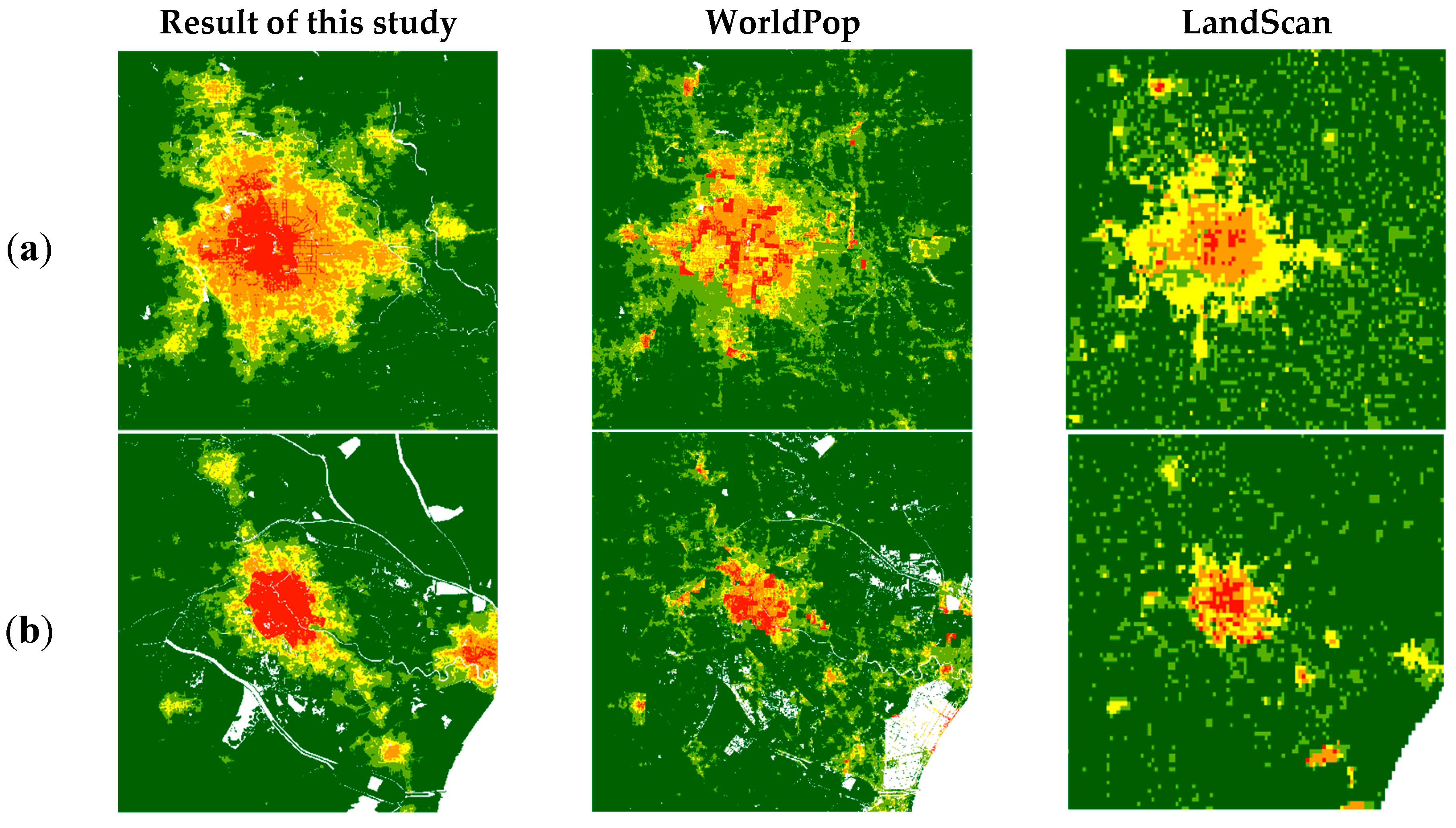
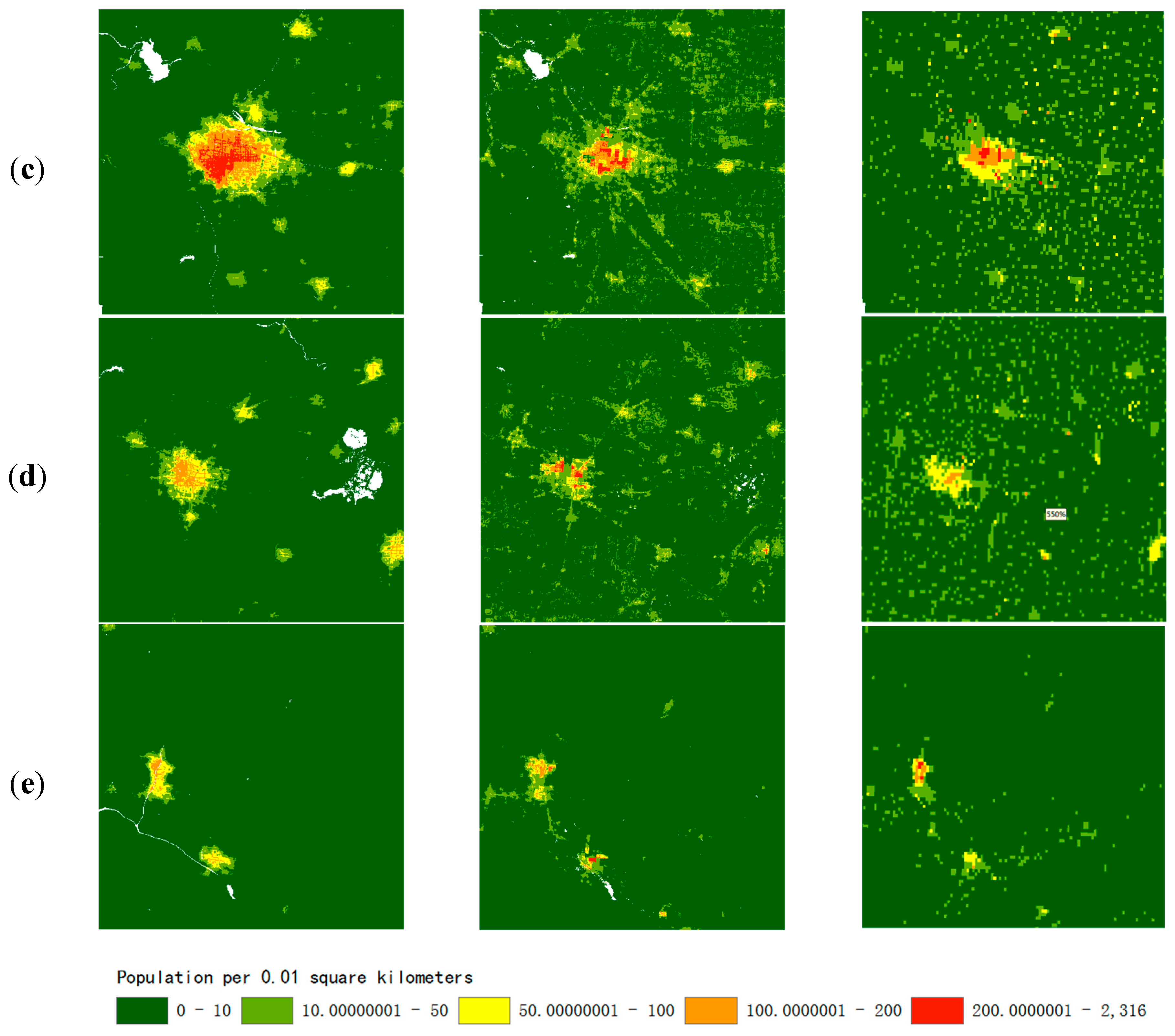
Figure 6.
Five regions with different population density in experimental area. (a) Beijing, (b) Tianjin, (c) Shijiazhuang, (d) Baoding, and (e) Zhangjiakou.
Figure 6.
Five regions with different population density in experimental area. (a) Beijing, (b) Tianjin, (c) Shijiazhuang, (d) Baoding, and (e) Zhangjiakou.

Figure 7.
Comparison of different datasets in typical areas. (a) Beijing, (b) Tianjin, (c) Shijiazhuang, (d) Baoding, and (e) Zhangjiakou.
Figure 7.
Comparison of different datasets in typical areas. (a) Beijing, (b) Tianjin, (c) Shijiazhuang, (d) Baoding, and (e) Zhangjiakou.


Figure 8.
Fine-grained population map driven by the dasymetric model driven by PSP, all POI records, and no POI. (a) PSP (b) All POI (c) no POI.
Figure 8.
Fine-grained population map driven by the dasymetric model driven by PSP, all POI records, and no POI. (a) PSP (b) All POI (c) no POI.

Figure 9.
Scatter plots of the dasymetric model driven by PSP, all POI records and no POI. (a) PSP (b) All POI (c) no POI.
Figure 9.
Scatter plots of the dasymetric model driven by PSP, all POI records and no POI. (a) PSP (b) All POI (c) no POI.

Figure 10.
Fine-grained population map driven by the dasymetric model driven by PSP and HDI POI select by others (a) PSP (b) Bakillah (c) Yao.
Figure 10.
Fine-grained population map driven by the dasymetric model driven by PSP and HDI POI select by others (a) PSP (b) Bakillah (c) Yao.

Figure 11.
Scatter plots of dasymetric model driven by PSP and HDI POI select by others (a) PSP (b) Bakillah (c) Yao.
Figure 11.
Scatter plots of dasymetric model driven by PSP and HDI POI select by others (a) PSP (b) Bakillah (c) Yao.

Figure 12.
Scatter plots of results in this study and existing datasets. (a) Result of the PSP-driven dasymetric model, (b) the WorldPop dataset, and (c) the LandScan dataset.
Figure 12.
Scatter plots of results in this study and existing datasets. (a) Result of the PSP-driven dasymetric model, (b) the WorldPop dataset, and (c) the LandScan dataset.


Table 1.
Datasets used in this study.
| Covariate | Dataset | Year | Source |
|---|---|---|---|
| Covariates for dasymetric model | POI | 2018 | NavInfo |
| Demographic data | 2017 | National Bureau of Statistics of China | |
| Road/river network | 2017 | OpenStreetMap | |
| Water body | 2017 | OpenStreetMap | |
| VIIRS night-time lights | 2017 | National Oceanic and Atmospheric Administration | |
| Land use/land cover | 2017 | MODIS land cover product | |
| DEM | Shuttle Radar Topography Mission | ||
| Supplementary data for identification of PSP | Easygo population heat map | 2019 | Tencent |
| Comparison data for accuracy evaluation | WorldPop global per country dataset | 2017 | WorldPop |
| LandScan dataset | 2017 | Oak Ridge National Laboratory |
Table 2.
The number of point-of-interests (POIs) in each of the 15 categories.
| Category | Count |
|---|---|
| Catering | 212,584 |
| Residential community | 105,708 |
| Wholesale and retail | 537,495 |
| Automobile sales and service | 61,918 |
| Financial service | 57,929 |
| Education service | 89,922 |
| Health and social security | 58,975 |
| Sport and leisure | 71,295 |
| Communal facilities | 80,584 |
| Commercial facilities and services | 31,567 |
| Resident services | 203,470 |
| Corporation enterprises | 169,974 |
| Transportation and storage | 94,744 |
| Scientific research and technical services | 5934 |
| Agriculture, forestry, animal husbandry and fishery | 7193 |
Table 3.
The support and confidence of the association rule between population gathering points and each category of POI.
Table 3.
The support and confidence of the association rule between population gathering points and each category of POI.
| Category | Support | Confidence | POI Category |
|---|---|---|---|
| Catering | 127,317 | 0.0018 | PIP |
| Residential community | 44,036 | 0.0019 | PSP |
| Wholesale and retail | 241,575 | 0.0024 | PSP |
| Automobile sales and service | 8756 | 0.0032 | PIP |
| Financial service | 26,667 | 0.0175 | PIP |
| Education service | 48,680 | 0.0021 | PSP |
| Medical institution | 25,460 | 0.0019 | PIP |
| Sport and leisure | 27,215 | 0.0017 | PIP |
| Communal facilities | 23,399 | 0.0016 | PIP |
| Commercial facilities and services | 22,909 | 0.0014 | PIP |
| Resident services | 92,936 | 0.0019 | PSP |
| Corporation enterprises | 55,846 | 0.0016 | PIP |
| Transportation and storage | 27,453 | 0.0016 | PIP |
| Scientific research and technical services | 8982 | 0.0037 | PIP |
| Agriculture, forestry, animal husbandry and fishery | 179 | 0.0023 | PIP |
Table 4.
Accuracy assessment of the dasymetric model driven by PSP, all POI records, and no POI.
| Dataset | MAE | RMSE | %RMSE | |
|---|---|---|---|---|
| All areas | PSP | 27,184.41 | 45,224.44 | 0.73 |
| All POIs | 30,306.07 | 48,357.27 | 0.78 | |
| No POIs | 34,714.98 | 56,541.58 | 0.92 | |
| Areas with high population density (>10,896 people per square kilometer) | PSP | 25,062.33 | 37,805.92 | 0.4 |
| All POIs | 29,250.78 | 41,437.18 | 0.43 | |
| No POIs | 33,976.64 | 46,853.96 | 0.50 | |
| Areas with medium population density (473–10,896 people per square kilometer) | PSP | 39,419.90 | 61,436.59 | 0.87 |
| All POIs | 42,798.99 | 64,913.49 | 0.92 | |
| No POIs | 50,623.59 | 77,315.64 | 1.11 | |
| Areas with low population density (<473 people per square kilometer) | PSP | 13,486.79 | 20,125.82 | 1.13 |
| POI | 15,175.16 | 22,573.78 | 1.27 | |
| No POIs | 14,241.86 | 22,156.93 | 1.26 |
Table 5.
Accuracy assessment of the dasymetric model driven by PSP and HDI POIs selected by others.
| Dataset | MAE | RMSE | %RMSE | |
|---|---|---|---|---|
| All areas | this study | 27,184.41 | 45,224.44 | 0.73 |
| Bakillah | 29,354.45 | 48,477.28 | 0.79 | |
| Yao | 29,486.41 | 47,722.09 | 0.78 | |
| Areas with high population density (>10,896 people per square kilometer) | this study | 25,062.33 | 37,805.92 | 0.4 |
| Bakillah | 28,381.24 | 40,762.10 | 0.44 | |
| Yao | 26,925.14 | 39,663.29 | 0.43 | |
| Areas with medium population density (473–10,896 people per square kilometer) | this study | 39,419.90 | 61,436.59 | 0.87 |
| Bakillah | 42,411.09 | 66,267.28 | 0.95 | |
| Yao | 41,991.12 | 64,591.05 | 0.93 | |
| Areas with low population density (<473 people per square kilometer) | this study | 13,486.79 | 20,125.82 | 1.13 |
| Bakillah | 12,918.79 | 17,798.96 | 1.02 | |
| Yao | 15,374.73 | 21,342.01 | 1.22 |
Table 6.
Accuracy assessment of PSP-driven dasymetric model results in various regions and comparison with the two reference datasets.
Table 6.
Accuracy assessment of PSP-driven dasymetric model results in various regions and comparison with the two reference datasets.
| Dataset | MAE | RMSE | %RMSE | |
|---|---|---|---|---|
| All areas | this study | 27,184.41 | 45,224.44 | 0.73 |
| WorldPop | 30,166.15 | 57,371.96 | 0.93 | |
| LandScan | 27,718.18 | 47,808.29 | 0.78 | |
| Areas with high population density (>10,896 people per square kilometer) | this study | 25,062.33 | 37,805.92 | 0.4 |
| WorldPop | 32,071.36 | 46,726.39 | 0.49 | |
| LandScan | 29,959.35 | 42,793.74 | 0.45 | |
| Areas with medium population density (473–10,896 people per square kilometer) | this study | 39,419.90 | 61,436.59 | 0.87 |
| WorldPop | 44,770.49 | 80,585.57 | 1.15 | |
| LandScan | 37,524.14 | 63,854.93 | 0.91 | |
| Areas with low population density (<473 people per square kilometer) | this study | 13,486.79 | 20,125.82 | 1.13 |
| WorldPop | 9,934.12 | 17,355.83 | 0.97 | |
| LandScan | 12,883.17 | 20,111.55 | 1.13 |
© 2019 by the authors. Licensee MDPI, Basel, Switzerland. This article is an open access article distributed under the terms and conditions of the Creative Commons Attribution (CC BY) license (http://creativecommons.org/licenses/by/4.0/).
Share and Cite
MDPI and ACS Style
Zhao, Y.; Li, Q.; Zhang, Y.; Du, X. Improving the Accuracy of Fine-Grained Population Mapping Using Population-Sensitive POIs. Remote Sens. 2019, 11, 2502. https://0-doi-org.brum.beds.ac.uk/10.3390/rs11212502
AMA Style
Zhao Y, Li Q, Zhang Y, Du X. Improving the Accuracy of Fine-Grained Population Mapping Using Population-Sensitive POIs. Remote Sensing. 2019; 11(21):2502. https://0-doi-org.brum.beds.ac.uk/10.3390/rs11212502
Chicago/Turabian StyleZhao, Yuncong, Qiangzi Li, Yuan Zhang, and Xin Du. 2019. "Improving the Accuracy of Fine-Grained Population Mapping Using Population-Sensitive POIs" Remote Sensing 11, no. 21: 2502. https://0-doi-org.brum.beds.ac.uk/10.3390/rs11212502
Note that from the first issue of 2016, this journal uses article numbers instead of page numbers. See further details here.