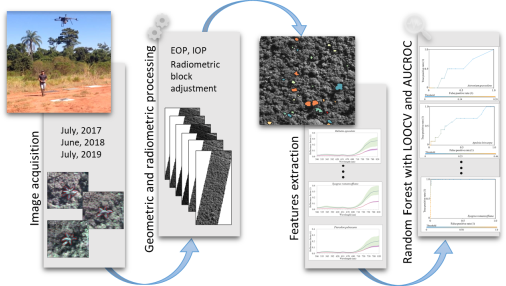
Article

Evaluation of Hyperspectral Multitemporal Information to Improve Tree Species Identification in the Highly Diverse Atlantic Forest

by
Gabriela Takahashi Miyoshi
1,*,
Nilton Nobuhiro Imai
1,2,
Antonio Maria Garcia Tommaselli
1,2,
Marcus Vinícius Antunes de Moraes
1 and
Eija Honkavaara
3
1
Graduate Program in Cartographic Sciences, São Paulo State University (UNESP), Roberto Simonsen 305, Presidente Prudente SP 19060-900, Brazil
2
Department of Cartography, São Paulo State University (UNESP), Roberto Simonsen 305, Presidente Prudente SP 19060-900, Brazil
3
Finnish Geospatial Research Institute, National Land Survey of Finland, Geodeetinrinne 2, 02430 Masala, Finland
*
Author to whom correspondence should be addressed.
Submission received: 13 November 2019 / Revised: 6 January 2020 / Accepted: 7 January 2020 / Published: 10 January 2020
(This article belongs to the Special Issue Mapping Tree Species Diversity)

Abstract

:
The monitoring of forest resources is crucial for their sustainable management, and tree species identification is one of the fundamental tasks in this process. Unmanned aerial vehicles (UAVs) and miniaturized lightweight sensors can rapidly provide accurate monitoring information. The objective of this study was to investigate the use of multitemporal, UAV-based hyperspectral imagery for tree species identification in the highly diverse Brazilian Atlantic forest. Datasets were captured over three years to identify eight different tree species. The study area comprised initial to medium successional stages of the Brazilian Atlantic forest. Images were acquired with a spatial resolution of 10 cm, and radiometric adjustment processing was performed to reduce the variations caused by different factors, such as the geometry of acquisition. The random forest classification method was applied in a region-based classification approach with leave-one-out cross-validation, followed by computing the area under the receiver operating characteristic (AUCROC) curve. When using each dataset alone, the influence of different weather behaviors on tree species identification was evident. When combining all datasets and minimizing illumination differences over each tree crown, the identification of three tree species was improved. These results show that UAV-based, hyperspectral, multitemporal remote sensing imagery is a promising tool for tree species identification in tropical forests.

Graphical Abstract

1. Introduction

Forests play an important role in biodiversity, carbon stocks, the water cycle, and feedstock, but they are rapidly being degraded. Knowledge about the tree species of a forest is fundamental information. Tree species mapping can be performed through fieldwork campaigns, but generally, this practice has limitations, since it is expensive and laborious. Remote sensing, together with automatic analysis techniques, has become a prominent tool for tree species mapping.
Satellite sensors [1] and airborne passive and/or active sensors [2,3], combined with the use of field spectroscopy [4], provide valuable information for the identification of tree species. Support vector machine (SVM) [5] and random forest (RF) [6] are examples of machine learning algorithms that have been successfully applied to identify tree species in urban environments [7], savannas [2], and different types of forests, including northern, boreal, temperate, and tropical forests [1,8,9,10,11,12]. Recently, these algorithms, with images acquired using unmanned aerial vehicles (UAVs), have become a powerful tool for forest monitoring [13,14,15].
UAVs enable fast information acquisition, and despite their constraints regarding the trade-off between resolution and coverage, they are low-cost alternatives for capturing information in areas that are endangered or need constant monitoring, such as mines or agricultural crops. UAVs can fly over many areas that are challenging for field data acquisition, such as water surfaces or dense forest areas. UAV missions can be quickly configured according to the user’s needs. Furthermore, in the past few years, UAVs have been rapidly developed to fly for several hours; an example of such a platform is the fixed-wing Batmap II UAV, which is able to fly for more than 2 h [16]. UAVs can capture very high or ultrahigh spatial resolution data with ground sampling distances (GSD) ranging from centimeters to decimeters [17,18,19,20] using small-format multispectral or hyperspectral cameras, such as MicaSense RedEdge-MX [21], Rikola hyperspectral imager [22], and Cubert FireflEYE [21]. Beyond that, UAVs can repeatedly acquire information through surface targets, such as trees, which is a highly promising option in forest monitoring, since it can measure dynamic phenological behavior according to seasons and tree characteristics.
Although most of the previous studies conducted with multiseasonal information have not employed UAVs, they have shown spectral differences within tree species and reported whether the tree species classification was improved [7,23,24,25,26,27,28,29,30]. Moreover, most of them have been performed in northern forests [31]. There is a lack of studies in forests such as the Brazilian Atlantic forest, which encompasses different ecosystems, such as mixed ombrophilous, dense ombrophilous, open ombrophilous, semideciduous seasonal, and deciduous seasonal forests [32]. Sothe et al. [14] studied a mixed ombrophilous forest whose characteristics differ from those of other types of Brazilian Atlantic forest, especially the semideciduous and deciduous seasonal forests. Their floristic compositions and forest structure are different [32], which highlights the importance of studying them separately.
In addition to their application in northern forests in which coniferous tree species are predominant, most studies have investigated well-developed forests or forests in which trees with different heights are spatially distinguished. Plots containing tree species in different development stages can present similar heights, and thereby cause spectral mixing due to leaf mixture and the effect of neighborhood spectra, since the number of emergent trees is smaller. Notwithstanding the importance of monitoring mature forests, monitoring fragments that are in the initial regeneration process is considered a key element in the connection of forest patches, and contributes to the maintenance of biodiversity [33,34].
The objective of this study was to develop and assess UAV-based remote sensing techniques to improve tree species identification in Brazilian Atlantic forest areas with vegetation stages that range from initial to advanced restoration. A further objective was to study whether multitemporal spectral information acquired over multiple years in the same season but under different moisture conditions could improve tree species classification. UAV-based hyperspectral images were acquired over three years during the winter season. Additionally, the classification performance of two different spectral features was compared. The findings in this paper are expected to provide information about the use of spectral features with minimized effects from illumination differences to classify tree species in the highly diverse Brazilian Atlantic forest, and demonstrate the use of hyperspectral multitemporal information.

2. Materials and Methods

2.1. Study Site

The transect forest sample used in this study is centered at 22°23′55.21″S, 52°31′18.31″W, in the municipality of Euclides da Cunha Paulista, western part of São Paulo State, Brazil (Figure 1). The transect has an approximate length and width of 500 m × 130 m, and comprises a variety of tree species in different successional stages. The study area was established inside the Ponte Branca forest fragment, a protected area belonging to the Black Lion Tamarin Ecological Station. According to the Brazilian Institute for Geography and Statistics (IBGE), it is an area of the submontane, semideciduous seasonal forest [35]. The regional climate is considered a tropical zone with dry winters (Aw), according to the Köppen classification [36]. The mean temperature during the dry season is 21 °C, with less than 60 mm of total precipitation [37]. The weather patterns differed between the years 2017, 2018, and 2019 and the flight campaigns (Figure 2). The season was wetter in 2017, with precipitation of 69 mm before the flight campaign, whereas the precipitation was 18.6 mm before the flight campaign of 2018 and 51 mm before the flight campaign of 2019; however, rain did not occur for at least 8 days before image acquisition [37].

2.2. Reference Data

More than 25 tree species with a diameter at breast height (DBH) greater than 3.8 cm were detected during fieldwork [38]. Tree species were in different successional stages, with the northernmost part of the study area containing trees in the initial stage of succession and the southernmost in a more advanced stage [
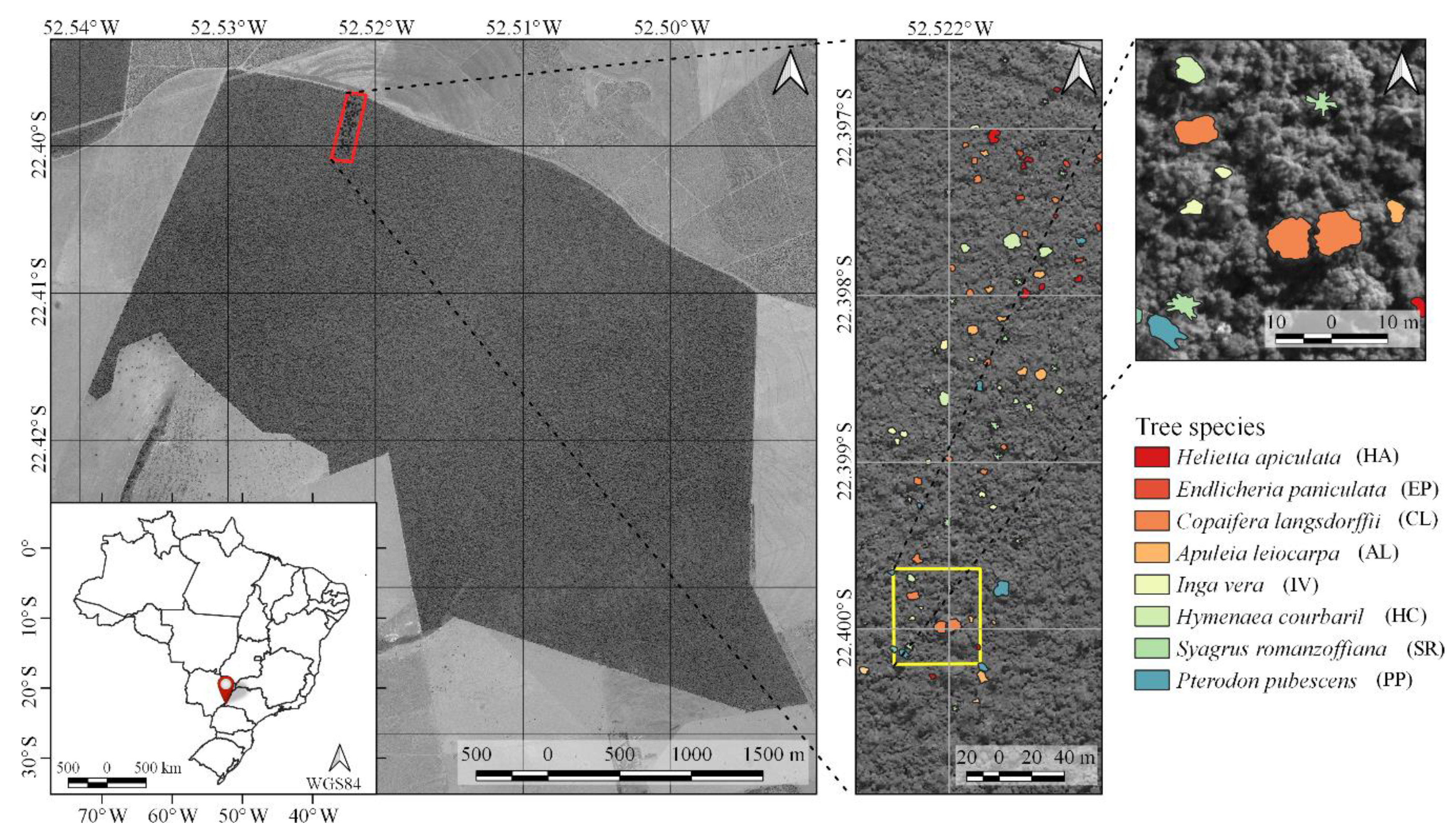
39]. Moreover, we located 90 trees of eight species that emerged from the canopy (Table 1 and 
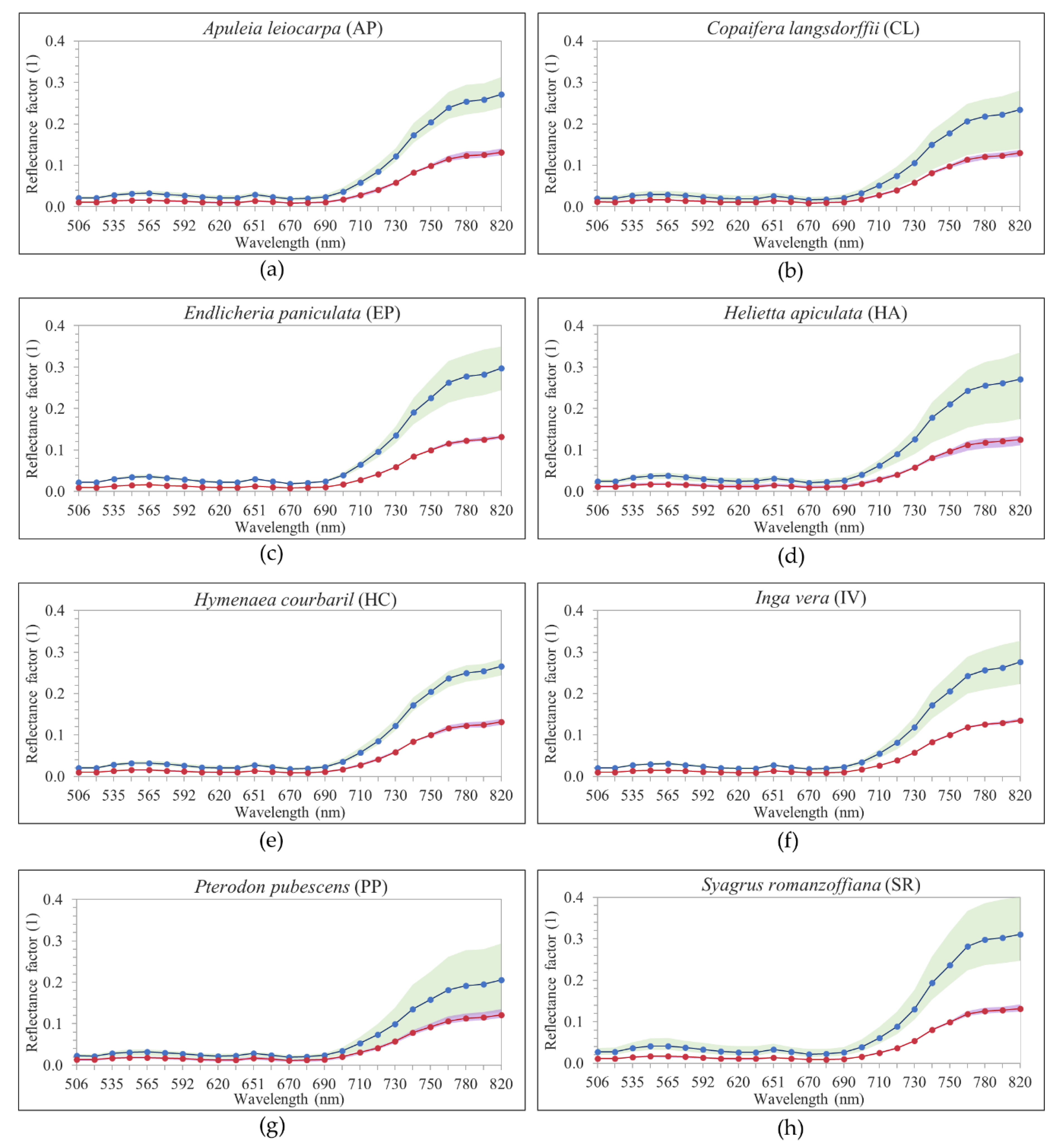
Table 2). Their crowns were manually delineated through visual interpretation of RGB image composites of each dataset (R: 628.73 nm; G: 550.39 nm; B: 506.22 nm). 
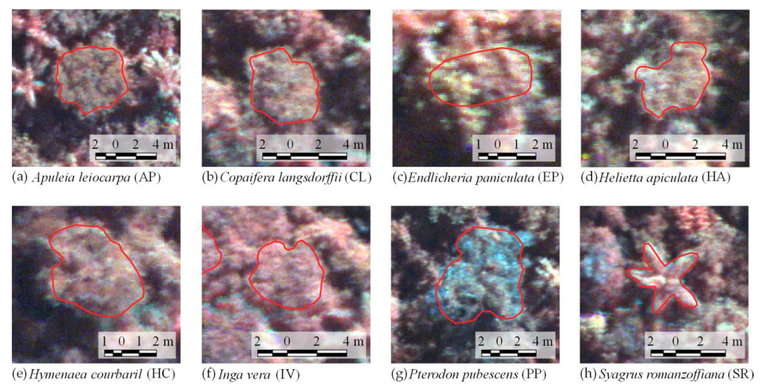
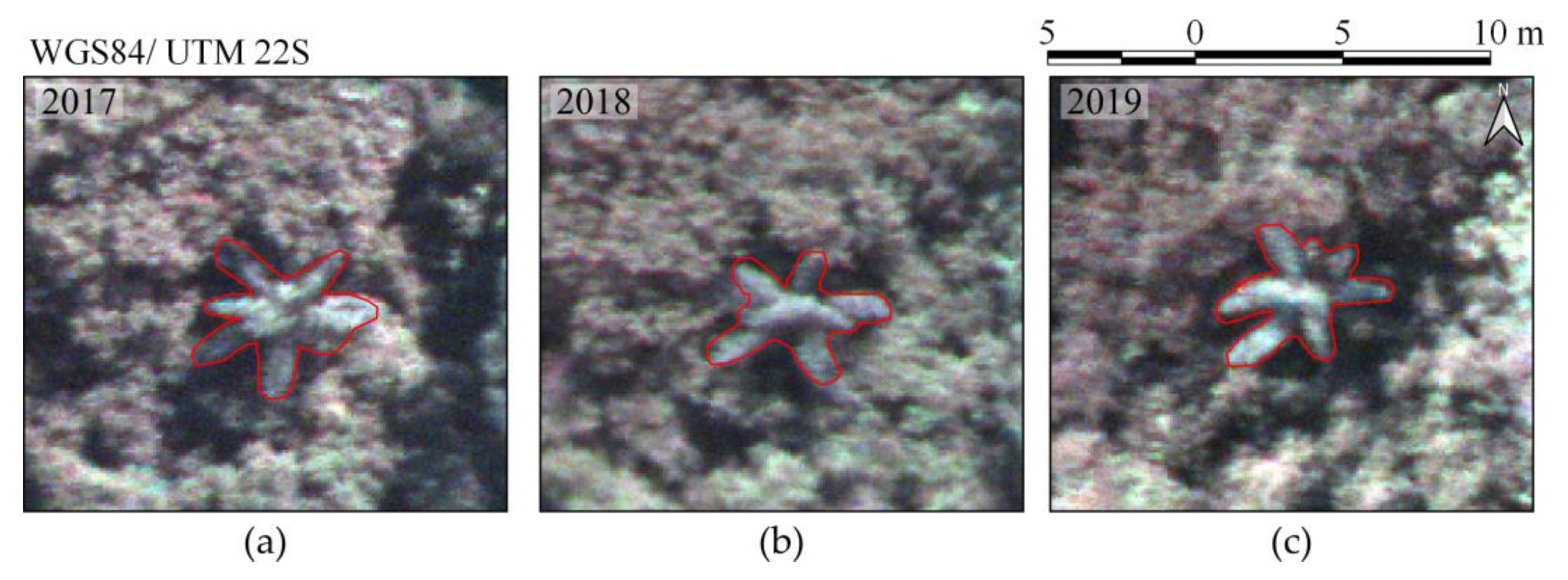
Figure 1 shows examples of delineated individual tree crown (ITC) polygons in the 2017 dataset, and 
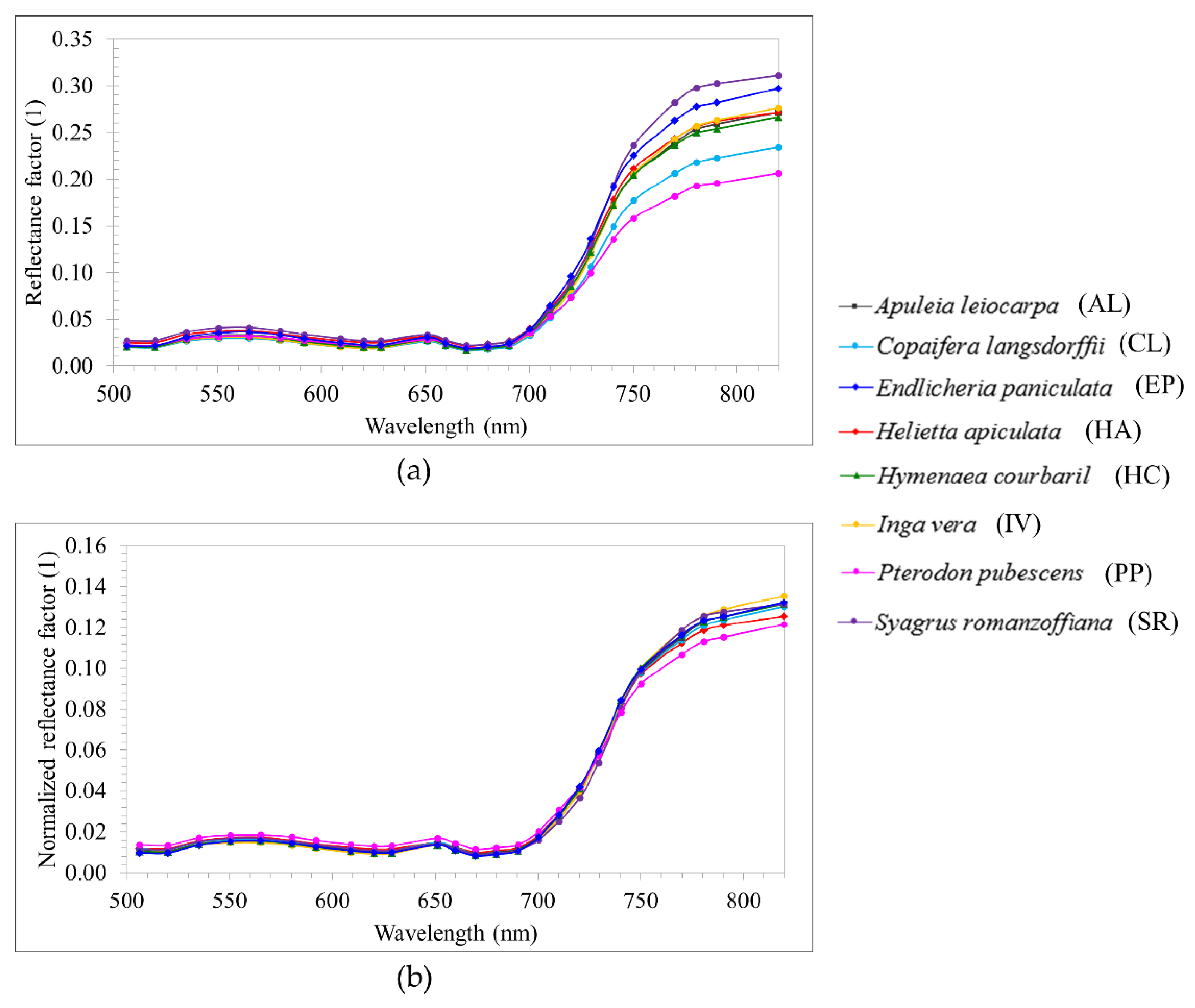
Figure 3 shows canopy examples of each tree species in the mosaic of images acquired during the 2017 flight campaign. These tree species were chosen because they are important for characterizing the successional stage of the forest, e.g., Syagrus romanzoffiana (SR), which can be associated with the faunal composition [40]. It is important to note that smaller tree species were excluded from analysis because the lianas that cover and mix among individuals negatively affect the classification accuracy. From now on, tree species will be called by their abbreviations from Table 1 and Table 2.
The number of samples was low for some species because of challenges in acquiring reference data. First, our study area comprised different successional stages; thus, the species composition varied over the area. Second, we used tree samples that emerged from the canopy. In tropical forests, the tree heights can be modeled by the DBH, which can be related to the number of trees per hectare [43,44,45]. According to Lima et al. [44] and d’Oliveira et al. [45], the relationship between the DBH and the frequency of trees in tropical forests has an “inverted J shape”, because the number of trees per hectare decreases substantially as the DBH increases, so the number of taller trees also decreases.

2.3. Remote Sensing Data

Hyperspectral images were acquired with a 2D-format camera based on the tunable Fabry–Pérot Interferometer (FPI) from Senop Ltd, model DT-0011 [46,47,
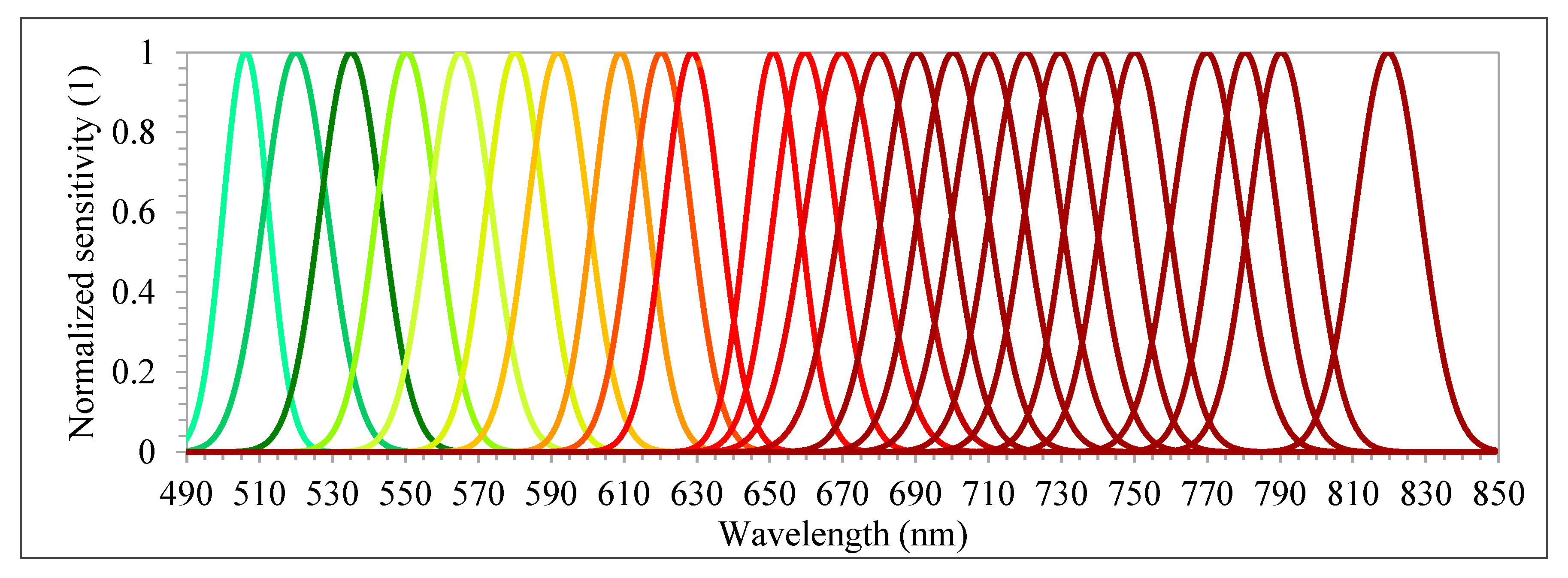
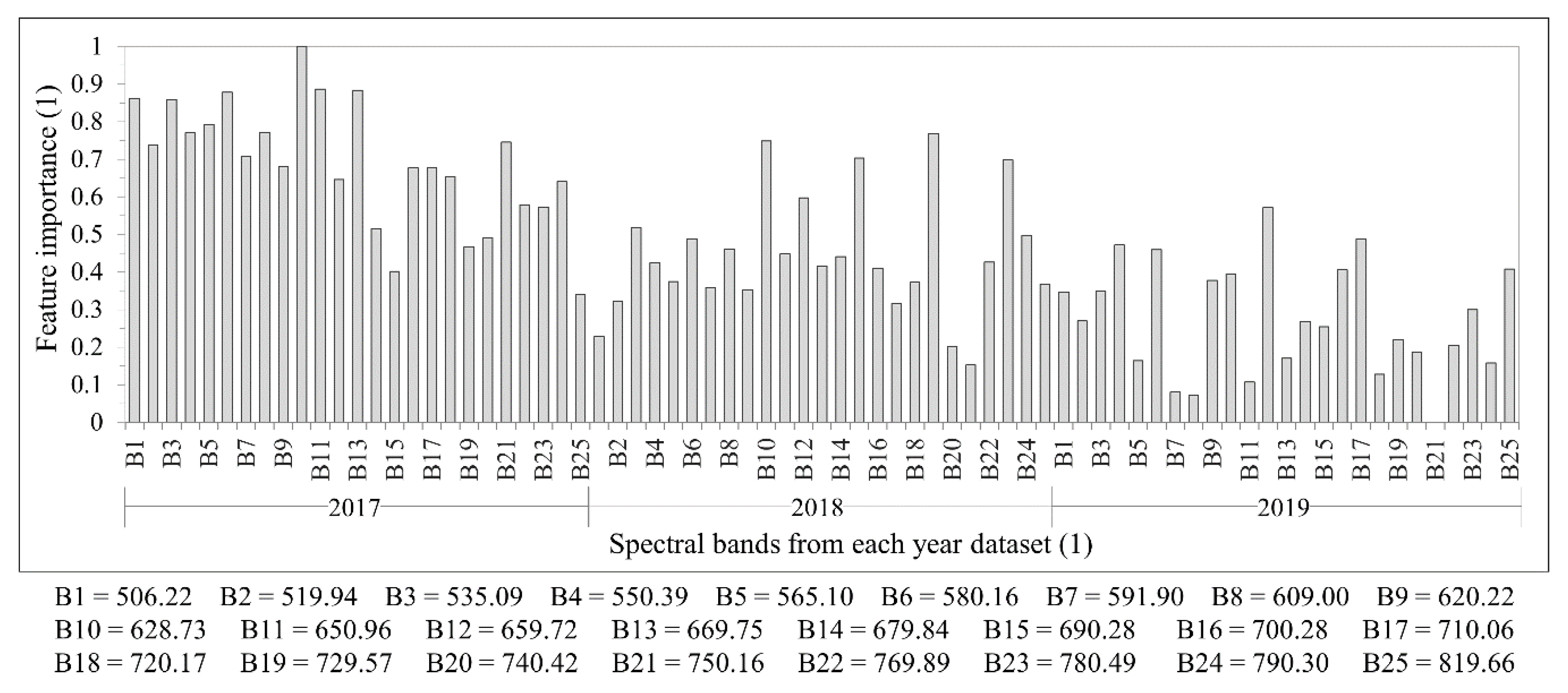
48]. The camera has two sensors, both of which have 1017 × 648 pixels with a pixel size of 5.5 µm. The total weight of the camera is around 700 g with its accessories, which include an irradiance sensor and a Global Positioning System (GPS) receiver. Spectral bands can be selected from the visible (VIS) to near-infrared (NIR) region (500–900 nm), which are acquired sequentially, i.e., the air gap of the FPI moves to acquire the different spectral bands of the same image. The spectral range of the first and second sensors are 647–900 nm and 500–635 nm, respectively. A total of 25 spectral bands were chosen, with the Full-Width at Half Maximum (FWHM) varying from 12.44 to 20.45 nm (Table 3 and Figure 4). For this spectral setting, each image cube needs 0.779 s to be acquired. The exposure time was set to 5 ms, and the image blocks were divided into two flight strips, ensuring more than 70% and 50% forward and side overlaps, respectively.
The FPI camera was mounted onboard the UX4 UAV, which is a rotary-wing quadcopter developed by the company Nuvem UAV. The UX4 UAV is almost 90 cm in diameter and 30 cm in height without counting the GPS antenna, which is approximately 15 cm. It is controlled by a PixHawk autopilot. The energy source for the UAV system and its sensors is one six-cell battery of 22 volts and one smaller three-cell battery of 11 volts, which allow the UAV to fly for up to 30 min, depending on payload, battery, and weather conditions. A flight speed of 4 m/s was used to limit the maximum gap between the first and last band of the hyperspectral imager to 3.1 m in a single cube.
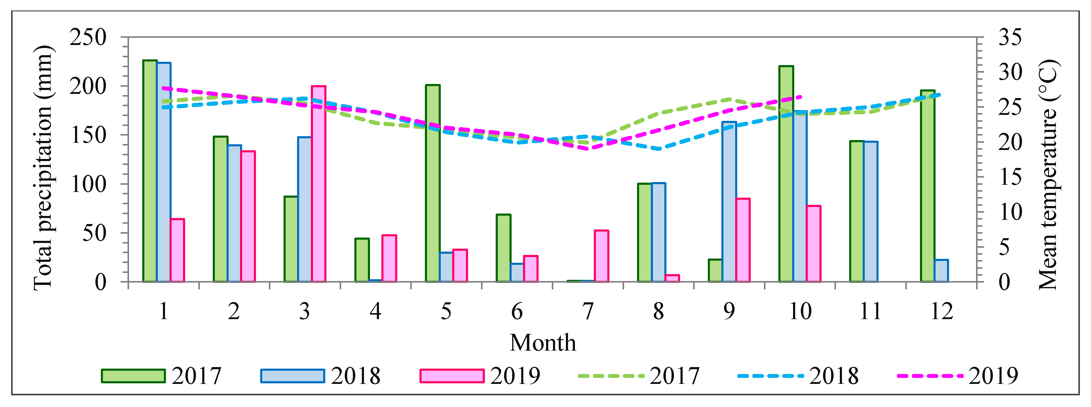
During the field campaigns, three radiometric reference targets were placed in the area to enable reflectance calibration. Flight campaigns were performed over the study area (Figure 1) on 1 July 2017, 16 June 2018, and 13 July 2019, with an above-ground flight height of approximately 160 m and flight speed of 4 m/s. The flight height was selected so that a GSD of 10 cm was obtained. This ensured a good representation of tree crowns that were predominantly over 3 m in diameter. Table 4 provides more details about the flight time of each campaign and the mean zenith and azimuth angles of the Sun during the image acquisitions.
Images were geometrically and radiometrically processed to obtain hyperspectral image orthomosaics. First, the images were radiometrically corrected from the dark current and nonuniformity of sensors using a dark image acquired before each flight and laboratory parameters [47,49].
The geometric processing was performed using the Agisoft PhotoScan software (version 1.3) (Agisoft LLC, St. Petersburg, Russia). In the orientation process, for each year, the exterior orientation parameters (EOPs) of four reference bands (band 3: 550.39 nm; band 8: 609.00 nm; band 14: 679.84 nm; and band 22: 769.89 nm) were estimated in the same Agisoft PhotoScan project in order to reduce misregistration between the datasets. The EOPs of the other bands were calculated using the method developed in [49,50]. Positions from the camera GPS were used as initial values and refined using a bundle block adjustment (BBA) and ground control points (GCPs). The number of GCPs varied between datasets, with 3, 3, and 4 used in 2017, 2018, and 2019, respectively. GCPs were placed outside the forest since it was not possible to see the ground from imagery acquired over the forested area. Initially, the base station was defined near the study area, and the global navigation satellite system (GNSS) observations from GCPs were collected and processed in differential mode.
A self-calibrating bundle adjustment was used to estimate the interior orientation parameters (IOPs) of each sensor and for each year of the dataset. After initial image alignment, parameter estimation was optimized with automatic outlier removal using a gradual selection of tie points based on reconstruction uncertainty and reprojection error, together with the manual removal of points. The final products of this step were the calibrated IOPs, EOPs, sparse and dense point clouds, and digital surface model (DSM) of the area with a GSD of 10 cm. These were used in the following radiometric block adjustment and mosaic generation.
Radiometric adjustment processing aims to correct the digital number (DN) of pixels of images from the bidirectional reflectance distribution function (BRDF) effects and differences caused by the different geometries of acquisition due to the UAV and Sun movements. Thus, nonuniformities among images were compensated for by the radBA software, developed at the Finnish Geospatial Research Institute (FGI) [49,50]. Equation (1) shows the model used in the software to extract the reflectance value from the DN of each pixel.
D N j k = a r e l j ( a a b s · R j k ( θ i , θ r , φ ) + b a b s ) ,
where D N j k is the digital number of pixel k in image j ; R j k ( θ i , θ r , φ ) is the corresponding reflectance factor with respect to the zenithal angle θ of the incident and reflected light, i and r , respectively, and with the relative azimuthal angle φ   ( φ r φ i ) , where φ r refers to the reflected azimuthal angle, and φ i denotes the incident azimuthal angle; a r e l j is the relative correction factor of illumination differences with respect to the reference image; and a a b s and b a b s are the empirical line parameters for the linear transformation between reflectance and DNs.
According to a previous study by Miyoshi et al. [47], for the study area, the best initial relative correction factor ( a r e l j ) was one (1), with a standard deviation equal to 0.05. It is worth noting that an exception was necessary for the dataset from 2018 because of higher density differences in cloud covering. The 2017 and 2019 flights were carried out in almost blue-sky conditions, with slight differences compensated for by the radiometric block adjustment. The radiometric block adjustment was performed in two steps for the 2018 dataset. First, an initial radiometric block adjustment was performed using initial values of a r e l j = 1. In sequence, the final values of a r e l j were used as the initial values for the second radiometric block adjustment. Then, the reflectance factor values were estimated using the empirical line method [51]. The empirical line parameters ( a a b s and b a b s ) were estimated from the linear relationship between the DN values of three radiometric reference targets with a mean reflectance of 4%, 11%, and 37%. Radiometric reference targets were 90 cm × 90 cm and composed of light-gray, gray, and black synthetic material. Thus, the mosaics of hyperspectral images for each dataset representing the reflectance factor values were obtained.
Additionally, point cloud data from airborne laser scanning (ALS) were provided by the company Fototerra. ALS data were acquired in November 2017 using a Riegl LMS-Q680i laser scanner (RIEGL, Horn, Austria) onboard a manned aircraft at a flight height of 400 m, which resulted in an average density of 8.4 points/m2. The canopy height model (CHM) was obtained by extracting the digital terrain model (DTM) from the DSM. The processing was performed using the LAStools software (Martin Isenburg, LAStools—efficient tools for LiDAR processing) [52]. First, the lasnoise tool was applied to withdraw possible noises in the point cloud. Then, the CHM was extracted using the lasheight tool to obtain tree heights in the study area.
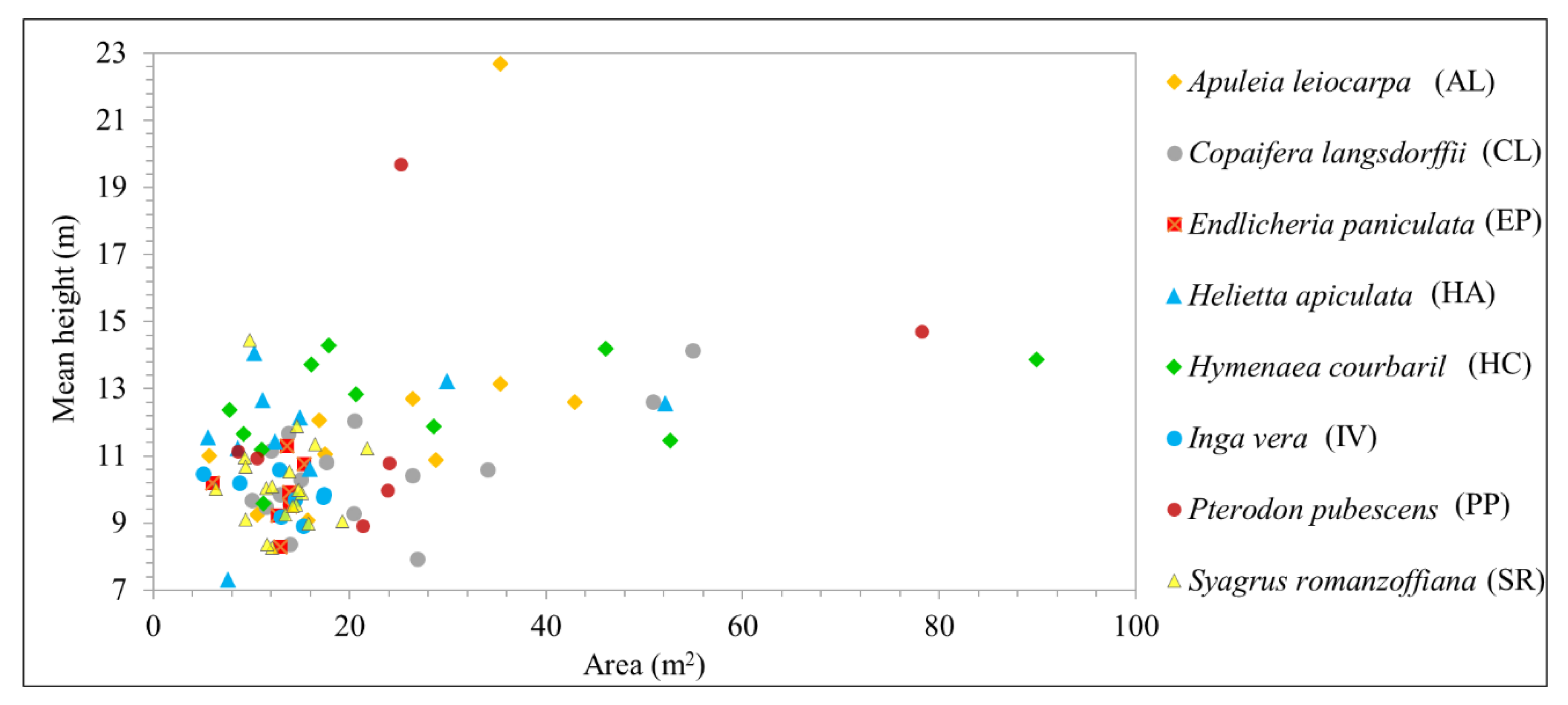
Figure 5 shows the mean height of each tree sample recognized in the field; most of the observed samples fell within a similar height range. Additionally, taller trees were found in the more developed successional stage of the area. Trees of the same species varied in age and were found in regions of different successional stages. For example, PP trees had crown areas of around 25 m2 and mean heights of 10–20 m. Similarly, HC samples had a mean height of almost 14 m, with tree crown areas ranging from 16 to 90 m2. It is important to highlight that the ALS data were not used in the classification step, since the objective of this research was to evaluate hyperspectral multitemporal data to improve tree species identification.

2.4. Extraction of Spectral Features

Spectral features were extracted using manually delineated crown polygons. We used spectral features taken from the reflectance mosaics and normalized features extracted after pixel normalization. The normalization reduced the differences between the sunlit and shadowed pixels, assuming a uniform distribution across the crown [13,53]. The normalization process was performed to reduce the spectral variability of spectra from the same tree species (within-species). The normalized pixel value was calculated by dividing the pixel value of a band by the sum of values of this pixel in all bands [53]. The mean values of normalized and nonnormalized pixels in each polygon were extracted for use in the region-based classification method. These values are referred to as MeanNorm and Mean, respectively.
Despite performing joint geometric processing, there were differences in the spatial position of trees, especially when using very high spatial resolution imagery. These differences are mainly caused by tree growth, changes in leaves with changing seasons, and weather conditions or projection differences due to the characteristics of the surface used. Figure 6 shows the slight difference in the spatial distribution of the leaves of SR trees.

2.5. Tree Species Identification with RF

The RF method was used for tree species identification using only the spectral information, since the objective was to verify whether the use of temporal information could improve tree species detection. This method is based on multiple decision trees, and the class is determined by the most popular vote [6]. Decision trees are composed of different samples, which are drawn with replacement, i.e., one sample can belong to more than one tree [54]. The RF has been successfully applied for image classification when working with high-dimensional data [8,13], and it is less sensitive to feature selection [54]. The RF was applied using the default parameters of the Weka software version 3.8.3 (The University of Waikato, Hamilton, New Zealand) [55].
The classification process was carried out five times with four different datasets: (i) the 2017 spectral information (D17); (ii) the 2018 spectral information (D18); (iii) the 2019 spectral information (D19); (iv) the combination of the 2017, 2018, and 2019 spectral information (Dall). For the D17, D18, and D19 datasets, we used the normalized pixel values to extract the spectral features, which are referred to as cases D17_MeanNorm, D18_MeanNorm, and D19_MeanNorm, respectively. Additionally, in the case of the combined dataset (item (iv) in the previously described datasets), the classification was performed using both the normalized and nominal values, referred to as Dall_MeanNorm and Dall_Mean, respectively. Table 5 summarizes the number of features used in each case.
The number of samples of different species is relatively low and also unbalanced. The leave-one-out cross-validation (LOOCV) method was used to circumvent this problem. LOOCV is a particular case of k-fold cross-validation, where k is equal to the total number of samples of the dataset [13,56]. The classification model is trained k times, followed by testing with one subset and training with the remaining subsets. In each iteration, the model is trained using k − 1 samples and tested with the remaining sample. The final accuracy values are obtained by averaging the accuracy values of each iteration [56]. LOOCV has been successfully applied in tree species classification studies with a small sample size (e.g., less than 10 samples per class [14]) or an unbalanced number of samples per class [13].
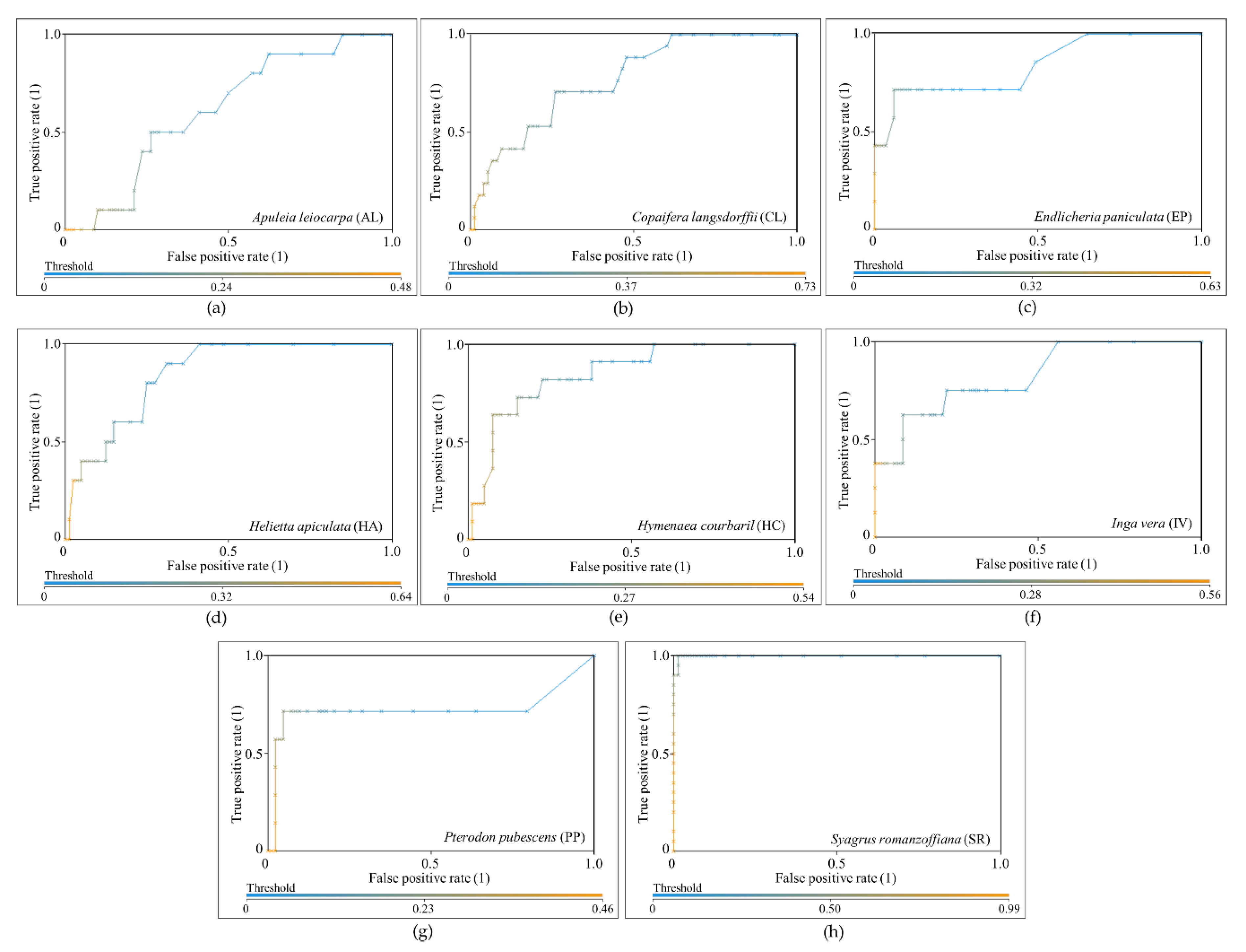
The results were evaluated through the area under the receiver operating characteristic curve, known as AUC (area under the curve) ROC (receiver operating characteristics) or AUCROC [57,58,59]. ROC is the relationship between the false positive rate (FPR), or “1-specificity”, and the true positive rate (TPR), or sensitivity, and it is useful when working with unbalanced classes because it is independent of the class distribution [59,60]. When using classifiers such as RF that provide probabilities or scores, thresholds can be applied to acquire different points in the ROC space to form an ROC curve [60]. AUCROC is the area under the ROC curve, and represents the probability of the classification model correctly classifying a random sample in a specific class. AUCROC varies from 0 to 1 for each class, where a value of 0.5 indicates that the specific classification model is no better than a random assignment, and a value of 1 represents perfect discrimination of a class from the remaining ones [59]. To the best classification (i.e., the one with highest value of average AUCROC value), the overall accuracy (i.e., the percentage of correctly classified instances of the total number of samples), the user accuracy, and the producer accuracy [61] were calculated as well.

3. Results

3.1. Spectral Response of Each Tree Species Recognized in the Field

The spectral variability within samples of the same tree species was verified through the mean, minimum, and maximum values of Mean and MeanNorm (defined in Section 2.3). The mean values are presented in Figure 7, showing similar spectral responses in the VIS region for both Mean and MeanNorm. In the NIR region, the Mean spectra are visually similar between IV, HA, HC, and AL. Despite smaller differences among the MeanNorm spectra, which may lead to higher classification confusion, the spectral variability within the samples of Mean had a higher range (Figure 8). In Figure 8, the range between the minimum and maximum values is visually the same for both the Mean and MeanNorm spectra of all tree species in the VIS part of the electromagnetic spectrum. It is noted that the number of samples of each tree species can affect this range of variation, as observed for SR with 20 samples. However, this behavior was not observed for AL (10 samples) and HC (11 samples). The range variation in the Mean values from the red-edge (700 nm) to near-infrared region (820 nm) had a higher variability when compared with the MeanNorm values, leading to the conclusion that a higher variability may influence classifier performance. Moreover, in Figure 7, an unusual peak may be noticed at the spectral response at 650 nm, probably due to the fact that this spectral band is located near the edge of the first sensor from the FPI, which acquires information from 647 nm to 900 nm.

3.2. Identification of Tree Species Results

Table 6 provides the AUCROC values after applying the RF with LOOCV to each dataset. Dall_MeanNorm presented the highest average AUCROC value (0.807), and thus, it can be considered the best dataset with which to identify the tree species. Average AUCROC values for Dall_Mean, D17_MeanNorm, D18_MeanNorm, and D19_MeanNorm were 0.783, 0.746, 0.754, and 0.682, respectively. Next, a more detailed analysis was performed using AUCROC values of Dall_MeanNorm.
Compared with the other datasets, Dall_MeanNorm had the highest AUCROC values for three of the eight tree species, namely, EP, HC, and SR. HA was better modeled in the D19_MeanNorm dataset, with an AUCROC value of 0.899, and it was worst modeled in the D18_MeanNorm dataset (AUCROC = 0.576). In contrast, IV was best and worst identified in D18_MeanNorm and D19_MeanNorm, respectively. Additionally, no significant differences were obtained when using normalized pixels compared with unnormalized ones for this tree species since the AUCROC values were 0.837 for Dall_Mean and 0.824 for Dall_MeanNorm. The identification of CL was similar between Dall_Mean (AUCROC = 0.742) and Dall_MeanNorm (AUCROC = 0.768), and it was best modeled in D17_MeanNorm (AUCROC = 0.821). AL had the lowest AUCROC value in D19_MeanNorm (0.313), which probably affected its identification in the Dall_MeanNorm dataset, in which its AUCROC was 0.613.
Since Dall_MeanNorm generated the best results in general, its ROC curves are shown in Figure 9, and its confusion matrix and user and producer accuracies are presented in Table 7. Figure 9 reveals different threshold values for each tree species, which are related to predictive probabilities [62]. For AL, which had the lowest AUCROC value (0.613), the FPR was higher than 0 (0.088), even when the TPR was equal 0, which indicates that the RF performed poorly in identifying this tree species, as confirmed by the confusion matrix, since none of AL were correctly identified. PP had the second lowest AUCROC value (0.723), and its threshold varied from 0 to 0.46, i.e., similar to AL. As shown in Figure 9 and in the confusion matrix of Table 7, only one tree species was correctly identified, and the TPR was only higher than 0 (TPR = 0.143) when the FPR was 0.024 to a threshold of 0.4. The highest AUCROC value, 0.999 for SR, corresponded to the tree species with the fewest false positives; that is, it was less frequently confused with the other tree species. The ROC curve of SR in Figure 9 shows that a TPR of 1 was obtained when the FPR was 0.014. This fact indicates that samples of this tree species will always be correctly identified; however, even with a low degree of variation, they could be confused with other tree samples, even in small proportions. Interestingly, for IV, that was not among the highest AUCROC values, the FPR is equal to 0 until a threshold of 0.44, when the TPR is 0.375. This fact is associated with the confusion matrix of Table 7, which has few false positives for this tree species.

Spectral Feature Importance

The feature importance in the Dall_MeanNorm dataset, which had the best classification results, is given in Figure 10. The feature importance was scaled from 0 to 1, where 0 represents the least important feature, and 1 represents the most important feature. The least important feature was band 21, centered at 750.16 nm, in the 2019 dataset, and the most important was band 10, centered at 628.73 nm, in the 2017 dataset. Additionally, in general, the most important features in the 2017 dataset were from the VIS part to the beginning of the red-edge part of the electromagnetic spectrum. In the 2018 dataset, an exception in feature importance may be observed at bands 15, 19, and 23, centered at 690.28 nm, 729.57 nm, and 780.49 nm. These bands were more important than most of the NIR bands in the 2018 dataset. In the 2019 dataset, bands 3, 6, and 12, centered at 535.09 nm, 580.16 nm, and 659.72 nm, respectively, were highlighted because of the peak in the feature importance value when compared with the other bands from 2019. These bands are in the VIS part of the electromagnetic spectrum; this is related to the leaves’ pigment, e.g., chlorophyll and carotenoids, content.

4. Discussion

Our study area is located in the highly diverse Brazilian Atlantic forest and comprises a great number of tree species at varying successional stages, which makes tree species identification in the field challenging. Most of the study area is in the initial stage of regeneration [39], which indicates that the tree heights have a low degree of variation, as verified in Figure 5. The southernmost part of the study area is more preserved and exhibits a medium degree of regeneration [39], as supported by the existence of taller trees in Figure 5. Monitoring this type of vegetation is a feasible way to increase the knowledge of forest composition and development, especially when the structural data do not have enough variation among classes to identify the tree species. The importance of regenerating forest paths is directly related to the maintenance of biodiversity.
The use of joint spectral normalized features (i.e., Dall_MeanNorm) increased the AUCROC values of three tree species (EP, HC, and SR). In general, when using the mean spectral features together (i.e., Dall_Mean), variations in the AUCROC values were more apparent compared with the use of spectral information from each dataset separately. The exception in the Dall_Mean results is to AL, whose AUCROC value increased with the use of temporal spectral information without normalization. Moreover, it was observed that weather conditions directly affected most of the trees’ phenology and, consequently, their spectral response, thus affecting RF performance on each dataset.
All the AUCROC values for SR were higher than 0.90, leading to the conclusion that the identification of this tree species did not depend on multitemporal information or the use of normalized spectra. A similar analysis can be applied to HC, which had similar AUCROC values in all tests, without counting the normalized spectra. CL had similar AUCROC values in Dall_Mean and Dall_MeanNorm and was better identified in D17_MeanNorm. Therefore, the weather pattern in 2017 was related to the identification accuracy of CL. There was a higher volume of rain before the 2017 flight campaign (Figure 2). Similarly, the weather influenced the detection of other tree species when using a single spectral dataset. The dry weather before the 2018 and 2019 flight campaigns hindered the ability to identify the AL tree species when using the spectral data of these years.
These tree species have different structures, such as the leaf format, and they have different blossom and fruit sets [41,42]. SR is a palm tree with leaves that are 2–3 m in length and spadices that are 80–120 cm in length [41]. HC has pinnate leaves and requires sunlight to grow and emerge from the canopy; blooming occurs in the dry season, and fruit appears after 3–4 months [42]. AL blooms without leaves, usually in September, and its flowers are white [42]. Thus, the use of multitemporal data influenced the detection of tree species. Of the previous works in the literature, the research of Ferreira et al. [28] is highlighted. They acquired WorldView images during the wet and dry seasons of a well-developed Brazilian semideciduous forest to classify tree species; no improvement in the classification results was observed when using the combined data. On the other hand, Somers and Asner [24], Deventer et al. [25], and Hill et al. [26] found that tree species classification improved when using multitemporal data because of the different spectral changes in the data.
As supported by previous research, VIS bands were among the most important features in tree species classification at the crown scale [10,13,63,64]. Vegetation spectra are characterized by the peak and absorption in the green and red parts of the electromagnetic spectrum, which is helpful for differentiating tree species. Similarly, the use of CHM has been shown to improve classification accuracies [13,14,65]. CHM data were not applied in our study since the focus was on the usefulness of temporal spectral information. The use of CHM data, combined with the use of tree crown segments, is highly recommended for future studies on the classification of tree species in the area.
This study was the first to investigate tree species classification using multitemporal hyperspectral UAV data acquired over the Atlantic forest. The previous studies that used multitemporal data acquired datasets from different seasons, and they did not use UAVs or consider a semideciduous forest with different development stages. Deventer et al. [25] simulated WorldView and RapidEye data from the leaf spectra of a subtropical forest in South Africa. Hill et al. [26] used the Daedalus 1268 AirborneThematic Mapper (ATM) sensor to acquire data over a deciduous forest in England. Using WorldView images, Li et al. [7] studied the multitemporal information of tree species in urban environments. When using UAVs, image acquisition depends on several factors (such as wind conditions since a UAV is a lightweight platform), and there are safety requirements to fulfill. During the spring and summer, when some trees may be blooming, the rainfall is higher; for example, summer rains may occur every day. Although images were acquired in the same season in this study, annual differences in tree phenology provided additional information and enhanced the classification accuracy.
The utilization of multitemporal data introduces some challenges to the data processing and classification processes. As shown in Figure 6, there are small differences in tree positions due to tree growth and probably also due to geometric projection characteristics; thus, trees were delineated separately in each dataset. When using structural features, the use of different polygons in the same point cloud might affect the classifier. Furthermore, these variations are challenging when working with very high spatial resolution imagery. Ferreira et al. [28] used resampled WorldView images at 0.30 and 1.2 m and needed to adjust the polygons of each ITC. Special attention must be paid to the radiometric processing of multitemporal spectral datasets. In this study, the datasets from each year were first processed to ensure that reflectance mosaics were uniform using the radiometric block adjustment, and further normalization of the shadows was shown to be advantageous.
Classification accuracies are always affected by the forest characteristics, the existence of several classes, and dataset characteristics, which should be considered for a reliable comparison of studies. Tuominen et al. [65] used multisource data to classify 26 different tree species of a Finnish forest into species and genus. They had more than 650 samples and achieved accuracies from 59.9% (when classifying tree species using the RF classifier and DN values of the shortwave infrared range) to 86.9% (when using selected features and the k-NN algorithm to classify the genus). Dalponte et al. [66] classified three types of trees in a boreal forest with more than 2300 samples and obtained an overall accuracy of 93.5% using manually delimited ITCs. Sothe et al. [14] used hyperspectral imagery and structural features to classify 12 tree species of a mixed ombrophilous forest, and achieved a maximum overall accuracy of 72.4%.
The number of samples affects the classification results and, thus, the analysis results, especially when using an unbalanced number of samples and statistics that consider the overall accuracy rather than the class accuracy. Therefore, the use of LOOCV followed by AUCROC analysis is extremely important because AUCROC values are specific to each class. In this study, the number of samples was quite low because of challenges in detecting the training data of a complex forest.
The delineation of the tree crown is equally important. When working with different successional stages and, thus, trees of potentially similar heights, correct spatial identification and tree crown delineation are crucial to the performance of any classifier. Since the region-based classification method provides better classification accuracy of tree species, future studies will be performed to fulfill this need. Approaches using ALS data have been successfully applied in boreal forests or pulpwood forests [67]. Wagner et al. [11] segmented the semideciduous Atlantic forest in a well-developed stage using imagery information only. Automating the delineation of the tree crown with acceptable accuracy would enhance the production of tree species maps to supplement forest monitoring.

5. Conclusions

The objective of this investigation was to develop hyperspectral unmanned aerial vehicle (UAV) imaging-based methods for tree species classification in an area of the Brazilian Atlantic forest that has great species diversity and a multitude of successional stages. An objective further was to assess the contribution of temporal spectral information to classification accuracy.
Temporal spectral information improved random forest performance for three of the eight tree species analyzed, indicating that promising accuracy could be obtained when using temporal spectral information. Separately analyzing single-date datasets showed that the weather patterns directly influenced the classification performance of some of the tree species. The analysis of datasets from several years of the same season showed that differences in weather conditions in different years resulted in some changes in the species spectra; these changes were useful for differentiating between tree species. The use of multitemporal spectra did not improve the identification of Inga vera, which had the highest area under the receiver operating characteristic curve (AUCROC) value when using only the dataset from 2018, and for Copaifera langsdorffii, which was better identified when using only the dataset from 2017. However, it is important to note that the AUCROC value for Apuleia leiocarpa resulting from the use of all the datasets (i.e., Dall_MeanNorm) might have been affected by the poor identification resulting from the use of the 2018 and 2019 datasets (AUCROC values equal 0.438 and 0.313, respectively). Weather conditions were observed to directly affect the tree species bloom because some species, such as Apuleia leiocarpa, bloom only in the dry season in trees that are completely without leaves. The normalization of spectra was necessary.
To the authors’ knowledge, this is the first work to use hyperspectral UAV images acquired over several years to classify the highly diverse Atlantic Forest. Improvements should be applied regarding the number of samples per class and the automated segmentation of individual tree crowns to enhance the applicability of the methodology, in addition to the use of tree height information. Moreover, care should be taken when using very high spatial resolution and automatic tree crown segmentation because of the slightly different positions of tree leaves caused by tree development.

Author Contributions

Conceptualization, G.T.M., N.N.I., and A.M.G.T.; data collection, G.T.M., N.N.I., A.M.G.T., M.V.A.d.M.; methodology, G.T.M., N.N.I., A.M.G.T., M.V.A.d.M., E.H.; writing—original draft preparation, G.T.M.; writing—review and editing, G.T.M., N.N.I., A.M.G.T., M.V.A.d.M., E.H.; supervision: N.N.I.; funding acquisition, N.N.I., A.M.G.T., E.H. All authors have read and agreed to the published version of the manuscript.

Funding

This study was financed in part by the Coordenação de Aperfeiçoamento de Pessoal de Nível Superior—Brasil (CAPES)—Finance Code 001 (process number 88881.187406/2018-01); in part by the National Council for Scientific and Technological Development (CNPq), grant number 153854/2016-2; in part by the São Paulo Research Foundation (FAPESP), grant number 2013/50426-4; and in part by the Academy of Finland, grant number 327861.

Acknowledgments

The authors would like to thank the company Fototerra S.A., through the individual César Francisco de Paula, for providing the ALS point cloud from the study area, as well as Valter Ribeiro Campos and the members of the Photogrammetry group from São Paulo State University (UNESP) who helped us during the fieldwork.

Conflicts of Interest

The authors declare no conflict of interest.

References

  1. Immitzer, M.; Atzberger, C.; Koukal, T. Tree Species Classification with Random Forest Using Very High Spatial Resolution 8-Band WorldView-2 Satellite Data. Remote Sens. 2012, 4, 2661–2693. [Google Scholar] [CrossRef] [Green Version]
  2. Colgan, M.S.; Baldeck, C.A.; Féret, J.-B.; Asner, G.P. Mapping Savanna Tree Species at Ecosystem Scales Using Support Vector Machine Classification and BRDF Correction on Airborne Hyperspectral and LiDAR Data. Remote Sens. 2012, 4, 3462–3480. [Google Scholar] [CrossRef] [Green Version]
  3. Heinzel, J.; Koch, B. Investigating multiple data sources for tree species classification in temperate forest and use for single tree delineation. Int. J. Appl. Earth Obs. Geoinf. 2012, 18, 101–110. [Google Scholar] [CrossRef]
  4. Zhang, C.; Chen, K.; Liu, Y.; Kovacs, J.M.; Flores-Verdugo, F.; de Santiago, F.J.F. Spectral response to varying levels of leaf pigments collected from a degraded mangrove forest. J. Appl. Remote Sens. 2012, 6, 063501. [Google Scholar]
  5. Melgani, F.; Bruzzone, L. Classification of hyperspectral remote sensing images with support vector machines. IEEE Trans. Geosci. Remote Sens. 2004, 42, 1778–1790. [Google Scholar] [CrossRef] [Green Version]
  6. Breiman, L. Random forests. Mach. Learn. 2001, 45, 5–32. [Google Scholar] [CrossRef] [Green Version]
  7. Li, D.; Ke, Y.; Gong, H.; Li, X. Object-Based Urban Tree Species Classification Using Bi-Temporal WorldView-2 and WorldView-3 Images. Remote Sens. 2015, 7, 16917–16937. [Google Scholar] [CrossRef] [Green Version]
  8. Maschler, J.; Atzberger, C.; Immitzer, M. Individual Tree Crown Segmentation and Classification of 13 Tree Species Using Airborne Hyperspectral Data. Remote Sens. 2018, 10, 1218. [Google Scholar] [CrossRef] [Green Version]
  9. Matsuki, T.; Yokoya, N.; Iwasaki, A. Hyperspectral Tree Species Classification of Japanese Complex Mixed Forest with the Aid of Lidar Data. IEEE J. Sel. Top. Appl. Earth Obs. Remote Sens. 2015, 8, 2177–2187. [Google Scholar] [CrossRef]
  10. Ferreira, M.P.; Zortea, M.; Zanotta, D.C.; Shimabukuro, Y.E.; de Souza Filho, C.R. Mapping tree species in tropical seasonal semi-deciduous forests with hyperspectral and multispectral data. Remote Sens. Environ. 2016, 179, 66–78. [Google Scholar] [CrossRef]
  11. Wagner, F.H.; Ferreira, M.P.; Sanchez, A.; Hirye, M.C.M.; Zortea, M.; Gloor, E.; Phillips, O.L.; Filho, C.R.; de Souza Filo, C.; Shimabukuro, Y.E.; et al. Individual tree crown delineation in a highly diverse tropical forest using very high resolution satellite images. ISPRS J. Photogramm. Remote Sens. 2018, 145, 362–377. [Google Scholar] [CrossRef]
  12. Feret, J.; Asner, G.P. Tree Species Discrimination in Tropical Forests Using Airborne Imaging Spectroscopy. IEEE Trans. Geosci. Remote Sens. 2013, 51, 73–84. [Google Scholar] [CrossRef]
  13. Nevalainen, O.; Honkavaara, E.; Tuominen, S.; Viljanen, N.; Hakala, T.; Yu, X.; Hyyppä, J.; Saari, H.; Pölönen, I.; Imai, N.N.; et al. Individual Tree Detection and Classification with UAV-Based Photogrammetric Point Clouds and Hyperspectral Imaging. Remote Sens. 2017, 9, 185. [Google Scholar] [CrossRef] [Green Version]
  14. Sothe, C.; Dalponte, M.; de Almeida, C.M.; Schimalski, M.B.; Lima, C.L.; Liesenberg, V.; Miyoshi, G.T.; Tommaselli, A.M.G. Tree Species Classification in a Highly Diverse Subtropical Forest Integrating UAV-Based Photogrammetric Point Cloud and Hyperspectral Data. Remote Sens. 2019, 11, 1338. [Google Scholar] [CrossRef] [Green Version]
  15. Otero, V.; Kerchove, R.V.D.; Satyanarayana, B.; Martínez-Espinosa, C.; Fisol, M.A.B.; Ibrahim, M.R.B.; Sulong, I.; Mohd-Lokman, H.; Lucas, R.; Dahdouh-Guebas, F. Managing mangrove forests from the sky: Forest inventory using field data and Unmanned Aerial Vehicle (UAV) imagery in the Matang Mangrove Forest Reserve, peninsular Malaysia. For. Ecol. Manag. 2018, 411, 35–45. [Google Scholar] [CrossRef]
  16. Nuvem UAV Batmap. Available online: http://nuvemuav.com/batmap (accessed on 5 December 2019).
  17. Aasen, H.; Honkavaara, E.; Lucieer, A.; Zarco-Tejada, P.J. Quantitative Remote Sensing at Ultra-High Resolution with UAV Spectroscopy: A Review of Sensor Technology, Measurement Procedures, and Data Correction Workflows. Remote Sens. 2018, 10, 1091. [Google Scholar] [CrossRef] [Green Version]
  18. Sanchez-Azofeifa, A.; Antonio Guzmán, J.; Campos, C.A.; Castro, S.; Garcia-Millan, V.; Nightingale, J.; Rankine, C. Twenty-first century remote sensing technologies are revolutionizing the study of tropical forests. Biotropica 2017, 49, 604–619. [Google Scholar] [CrossRef]
  19. Colomina, I.; Molina, P. Unmanned aerial systems for photogrammetry and remote sensing: A review. ISPRS J. Photogramm. Remote Sens. 2014, 92, 79–97. [Google Scholar] [CrossRef] [Green Version]
  20. Paneque-Gálvez, J.; McCall, M.K.; Napoletano, B.M.; Wich, S.A.; Koh, L.P. Small Drones for Community-Based Forest Monitoring: An Assessment of Their Feasibility and Potential in Tropical Areas. Forests 2014, 5, 1481–1507. [Google Scholar] [CrossRef] [Green Version]
  21. Cubert UAV Mapping with FireflEYE—Cubert. Available online: https://cubert-gmbh.com/applications/uav-mapping-with-firefleye/ (accessed on 25 October 2019).
  22. Senop Datasheet. Available online: https://senop.fi/files/rikola/pdf/Hyperspectral+Camera_Datasheet.pdf (accessed on 25 October 2019).
  23. Key, T.; Warner, T.A.; McGraw, J.B.; Fajvan, M.A. A Comparison of Multispectral and Multitemporal Information in High Spatial Resolution Imagery for Classification of Individual Tree Species in a Temperate Hardwood Forest. Remote Sens. Environ. 2001, 75, 100–112. [Google Scholar] [CrossRef]
  24. Somers, B.; Asner, G.P. Tree species mapping in tropical forests using multi-temporal imaging spectroscopy: Wavelength adaptive spectral mixture analysis. Int. J. Appl. Earth Obs. Geoinf. 2014, 31, 57–66. [Google Scholar] [CrossRef]
  25. Van Deventer, H.; Cho, M.A.; Mutanga, O. Improving the classification of six evergreen subtropical tree species with multi-season data from leaf spectra simulated to WorldView-2 and RapidEye. Int. J. Remote Sens. 2017, 38, 4804–4830. [Google Scholar] [CrossRef]
  26. Hill, R.A.; Wilson, A.K.; George, M.; Hinsley, S.A. Mapping tree species in temperate deciduous woodland using time-series multi-spectral data. Appl. Veg. Sci. 2010, 13, 86–99. [Google Scholar] [CrossRef]
  27. Castro-Esau, K.L.; Sánchez-Azofeifa, G.A.; Rivard, B.; Wright, S.J.; Quesada, M. Variability in leaf optical properties of Mesoamerican trees and the potential for species classification. Am. J. Bot. 2006, 93, 517–530. [Google Scholar] [CrossRef]
  28. Ferreira, M.P.; Wagner, F.H.; Aragão, L.E.O.C.; Shimabukuro, Y.E.; de Filho, C.R.S. Tree species classification in tropical forests using visible to shortwave infrared WorldView-3 images and texture analysis. ISPRS J. Photogramm. Remote Sens. 2019, 149, 119–131. [Google Scholar] [CrossRef]
  29. Karasiak, N.; Dejoux, J.-F.; Fauvel, M.; Willm, J.; Monteil, C.; Sheeren, D. Statistical Stability and Spatial Instability in Mapping Forest Tree Species by Comparing 9 Years of Satellite Image Time Series. Remote Sens. 2019, 11, 2512. [Google Scholar] [CrossRef] [Green Version]
  30. Immitzer, M.; Neuwirth, M.; Böck, S.; Brenner, H.; Vuolo, F.; Atzberger, C. Optimal Input Features for Tree Species Classification in Central Europe Based on Multi-Temporal Sentinel-2 Data. Remote Sens. 2019, 11, 2599. [Google Scholar] [CrossRef] [Green Version]
  31. Fassnacht, F.E.; Latifi, H.; Stereńczak, K.; Modzelewska, A.; Lefsky, M.; Waser, L.T.; Straub, C.; Ghosh, A. Review of studies on tree species classification from remotely sensed data. Remote Sens. Environ. 2016, 186, 64–87. [Google Scholar] [CrossRef]
  32. Available online: http://www.planalto.gov.br/ccivil_03/_Ato2004-2006/2006/Lei/L11428.htm (accessed on 10 September 2019).
  33. Ribeiro, M.C.; Metzger, J.P.; Martensen, A.C.; Ponzoni, F.J.; Hirota, M.M. The Brazilian Atlantic Forest: How much is left, and how is the remaining forest distributed? Implications for conservation. Biol. Conserv. 2009, 142, 1141–1153. [Google Scholar] [CrossRef]
  34. Lira, P.K.; Tambosi, L.R.; Ewers, R.M.; Metzger, J.P. Land-use and land-cover change in Atlantic Forest landscapes. For. Ecol. Manag. 2012, 278, 80–89. [Google Scholar] [CrossRef]
  35. Ibge Manual técnico da vegetação brasileira. Available online: https://biblioteca.ibge.gov.br/visualizacao/livros/liv63011.pdf (accessed on 25 May 2019).
  36. Alvares, C.A.; Stape, J.L.; Sentelhas, P.C.; de Moraes Gonçalves, J.L.; Sparovek, G. Köppen’s climate classification map for Brazil. Meteorol. Z. 2013, 22, 711–728. [Google Scholar] [CrossRef]
  37. INMET—Instituto Nacional de Meteorologia Estações Automáticas—Gráficos. Available online: http://www.inmet.gov.br/portal/index.php?r=home/page&page=rede_estacoes_auto_graf (accessed on 8 November 2019).
  38. Berveglieri, A.; Tommaselli, A.M.G.; Imai, N.N.; Ribeiro, E.A.W.; Guimarães, R.B.; Honkavaara, E. Identification of Successional Stages and Cover Changes of Tropical Forest Based on Digital Surface Model Analysis. IEEE J. Sel. Top. Appl. Earth Obs. Remote Sens. 2016, 9, 5385–5397. [Google Scholar] [CrossRef]
  39. Berveglieri, A.; Imai, N.N.; Tommaselli, A.M.G.; Casagrande, B.; Honkavaara, E. Successional stages and their evolution in tropical forests using multi-temporal photogrammetric surface models and superpixels. ISPRS J. Photogramm. Remote Sens. 2018, 146, 548–558. [Google Scholar] [CrossRef]
  40. Da Silva, F.R.; Begnini, R.M.; Lopes, B.C.; Castellani, T.T. Seed dispersal and predation in the palm Syagrus romanzoffiana on two islands with different faunal richness, southern Brazil. Stud. Neotropical Fauna Environ. 2011, 46, 163–171. [Google Scholar] [CrossRef]
  41. Lorenzi, H. Árvores brasileiras. In Plant. Nova Odessa, 1st ed.; Editora Plantarum: Nova Odessa, SP, Brazil, 1992; Volumes 1–2. [Google Scholar]
  42. Lorenzi, H. Árvores brasileiras. In Plant. Nova Odessa, 2nd ed.; Editora Plantarum: Nova Odessa, SP, Brazil, 1992; Volume 1. [Google Scholar]
  43. Da Scaranello, M.A.S.; Alves, L.F.; Vieira, S.A.; de Camargo, P.B.; Joly, C.A.; Martinelli, L.A. Height-diameter relationships of tropical Atlantic moist forest trees in southeastern Brazil. Sci. Agric. 2012, 69, 26–37. [Google Scholar] [CrossRef] [Green Version]
  44. Lima, R.B.; Bufalino, L.; Alves Junior, F.T.; da Silva, J.A.A.; Ferreira, R.L.C. Diameter distribution in a Brazilian tropical dry forest domain: Predictions for the stand and species. Anais Acad. Bras. Ciênc. 2017, 89, 1189–1203. [Google Scholar] [CrossRef] [Green Version]
  45. D’Oliveira, M.V.N.; Alvarado, E.C.; Santos, J.C.; Carvalho, J.A. Forest natural regeneration and biomass production after slash and burn in a seasonally dry forest in the Southern Brazilian Amazon. For. Ecol. Manag. 2011, 261, 1490–1498. [Google Scholar] [CrossRef]
  46. Miyoshi, G.; Imai, N.; Tommaselli, A.; Honkavaara, E. Comparison of Pixel and Region-Based Approaches for Tree Species Mapping in Atlantic Forest Using Hyperspectral Images Acquired by Uav. ISPRS-Int. Arch. Photogramm. Remote Sens. Spat. Inf. Sci. 2019, 4213, 1875–1880. [Google Scholar] [CrossRef] [Green Version]
  47. Miyoshi, G.T.; Imai, N.N.; Tommaselli, A.M.G.; Honkavaara, E.; Näsi, R.; Moriya, É.A.S. Radiometric block adjustment of hyperspectral image blocks in the Brazilian environment. Int. J. Remote Sens. 2018, 39, 4910–4930. [Google Scholar] [CrossRef] [Green Version]
  48. De Oliveira, R.A.; Tommaselli, A.M.G.; Honkavaara, E. Geometric Calibration of a Hyperspectral Frame Camera. Photogramm. Rec. 2016, 31, 325–347. [Google Scholar] [CrossRef]
  49. Honkavaara, E.; Saari, H.; Kaivosoja, J.; Pölönen, I.; Hakala, T.; Litkey, P.; Mäkynen, J.; Pesonen, L. Processing and Assessment of Spectrometric, Stereoscopic Imagery Collected Using a Lightweight UAV Spectral Camera for Precision Agriculture. Remote Sens. 2013, 5, 5006–5039. [Google Scholar] [CrossRef] [Green Version]
  50. Honkavaara, E.; Rosnell, T.; Oliveira, R.; Tommaselli, A. Band registration of tuneable frame format hyperspectral UAV imagers in complex scenes. ISPRS J. Photogramm. Remote Sens. 2017, 134, 96–109. [Google Scholar] [CrossRef]
  51. Smith, G.M.; Milton, E.J. The use of the empirical line method to calibrate remotely sensed data to reflectance. Int. J. Remote Sens. 1999, 20, 2653–2662. [Google Scholar] [CrossRef]
  52. Isenburg, M. Available online: http://lastools.org/ (accessed on 21 November 2018).
  53. Dalponte, M.; Frizzera, L.; Gianelle, D. Individual tree crown delineation and tree species classification with hyperspectral and LiDAR data. PeerJ 2019, 6, e6227. [Google Scholar] [CrossRef] [PubMed]
  54. Belgiu, M.; Drăguţ, L. Random forest in remote sensing: A review of applications and future directions. ISPRS J. Photogramm. Remote Sens. 2016, 114, 24–31. [Google Scholar] [CrossRef]
  55. Hall, M.; Frank, E.; Holmes, G.; Pfahringer, B.; Reutemann, P.; Witten, I.H. The WEKA data mining software: An update. SIGKDD Explor. 2009, 11, 10–18. [Google Scholar] [CrossRef]
  56. Brovelli, M.A.; Crespi, M.; Fratarcangeli, F.; Giannone, F.; Realini, E. Accuracy assessment of high resolution satellite imagery orientation by leave-one-out method. ISPRS J. Photogramm. Remote Sens. 2008, 63, 427–440. [Google Scholar] [CrossRef]
  57. Fan, J.; Upadhye, S.; Worster, A. Understanding receiver operating characteristic (ROC) curves. Can. J. Emerg. Med. 2006, 8, 19–20. [Google Scholar] [CrossRef]
  58. Bradley, A.P.; Duin, R.P.W.; Paclik, P.; Landgrebe, T.C.W.; Bradley, A.P.; Duin, R.P.W.; Paclik, P.; Landgrebe, T.C.W. Precision-recall operating characteristic (P-ROC) curves in imprecise environments. In Proceedings of the 18th International Conference on Pattern Recognition (ICPR’06), Hong Kong, China, 20–24 August 2006; Volume 4, pp. 123–127. [Google Scholar]
  59. Evangelista, P.H.; Stohlgren, T.J.; Morisette, J.T.; Kumar, S. Mapping Invasive Tamarisk (Tamarix): A Comparison of Single-Scene and Time-Series Analyses of Remotely Sensed Data. Remote Sens. 2009, 1, 519–533. [Google Scholar] [CrossRef] [Green Version]
  60. Fawcett, T. An introduction to ROC analysis. Pattern Recognit. Lett. 2006, 27, 861–874. [Google Scholar] [CrossRef]
  61. Li, W.; Guo, Q.; Jakubowski, M.K.; Kelly, M. A New Method for Segmenting Individual Trees from the Lidar Point Cloud. Photogramm. Eng. Remote Sens. 2012, 78, 75–84. [Google Scholar] [CrossRef] [Green Version]
  62. Witten, I.H.; Frank, E. Data Mining: Practical Machine Learning Tools and Techniques, 2nd ed.; Morgan Kaufmann Series in Data Management Systems; Morgan Kaufmann: San Francisco, CA, USA, 2005. [Google Scholar]
  63. Michez, A.; Piégay, H.; Lisein, J.; Claessens, H.; Lejeune, P. Classification of riparian forest species and health condition using multi-temporal and hyperspatial imagery from unmanned aerial system. Environ. Monit. Assess. 2016, 188, 146. [Google Scholar] [CrossRef] [PubMed] [Green Version]
  64. Clark, M.L.; Roberts, D.A.; Clark, D.B. Hyperspectral discrimination of tropical rain forest tree species at leaf to crown scales. Remote Sens. Environ. 2005, 96, 375–398. [Google Scholar] [CrossRef]
  65. Tuominen, S.; Näsi, R.; Honkavaara, E.; Balazs, A.; Hakala, T.; Viljanen, N.; Pölönen, I.; Saari, H.; Ojanen, H. Assessment of Classifiers and Remote Sensing Features of Hyperspectral Imagery and Stereo-Photogrammetric Point Clouds for Recognition of Tree Species in a Forest Area of High Species Diversity. Remote Sens. 2018, 10, 714. [Google Scholar] [CrossRef] [Green Version]
  66. Dalponte, M.; Ørka, H.O.; Ene, L.T.; Gobakken, T.; Næsset, E. Tree crown delineation and tree species classification in boreal forests using hyperspectral and ALS data. Remote Sens. Environ. 2014, 140, 306–317. [Google Scholar] [CrossRef]
  67. Kaartinen, H.; Hyyppä, J.; Yu, X.; Vastaranta, M.; Hyyppä, H.; Kukko, A.; Holopainen, M.; Heipke, C.; Hirschmugl, M.; Morsdorf, F.; et al. An International Comparison of Individual Tree Detection and Extraction Using Airborne Laser Scanning. Remote Sens. 2012, 4, 950–974. [Google Scholar] [CrossRef] [Green Version]
Figure 1. Study area and tree species recognized in the field in the 2017 dataset. The red rectangle represents the imaged area, and the yellow rectangle is a zoom of the study area.
Remotesensing 12 00244 g001
Figure 2. Climograph of Paranapoema station from the National Institute of Meteorology. Bars represent the accumulated rainfall per month (mm), and dashed lines represent the mean monthly temperature (°C).
Remotesensing 12 00244 g002
Figure 3. Canopy examples of each tree species identified in the field and delineated in the images acquired in 2017 (R: 780.49 nm; G: 565.10 nm; B: 506.22 nm; automatic contrast from QGIS software, version 3.0.0). (a) Apuleia leiocarpa (AP), (b) Copaifera langsdorffii (CL), (c) Endlicheria paniculata (EP), (d) Helietta apiculata (HA), (e) Hymenaea courbaril (HC), (f) Inga vera (IV), (g) Pterodon pubescens (PP), (h) Syagrus romanzoffiana (SR).
Remotesensing 12 00244 g003
Figure 4. Normalized sensitivities of each spectral band set in the FPI camera. Responses were calculated from the central wavelength and FWHM.
Remotesensing 12 00244 g004
Figure 5. Mean tree height versus the tree crown area for all samples identified in the field. Data are from the 2017 dataset.
Remotesensing 12 00244 g005
Figure 6. The spatial difference in the leaves of one sample of SR tree in each dataset (R: 690.28 nm; G: 565.10 nm; B: 519.94 nm; automatic contrast from QGIS software, version 3.0.0): (a) 2017, (b) 2018, and (c) 2019.
Remotesensing 12 00244 g006
Figure 7. Mean spectra of each tree species considering the: (a) Mean, and the (b) MeanNorm.
Remotesensing 12 00244 g007
Figure 8. Values for each tree species considering the mean reflectance factor spectra (Mean) and the mean normalized spectra (MeanNorm) calculated using pixels in the delineated crown polygons. The blue line represents the Mean, the red line represents the MeanNorm, and the shaded area represents the minimum and maximum values. (a) Apuleia leiocarpa (AP), (b) Copaifera langsdorffii (CL), (c) Endlicheria paniculata (EP), (d) Helietta apiculata (HA), (e) Hymenaea courbaril (HC), (f) Inga vera (IV), (g) Pterodon pubescens (PP), (h) Syagrus romanzoffiana (SR).
Remotesensing 12 00244 g008
Figure 9. ROC curves of the identification of each tree species from the application of RF to all imagery datasets (Dall_MeanNorm). (a) Apuleia leiocarpa (AP), (b) Copaifera langsdorffii (CL), (c) Endlicheria paniculata (EP), (d) Helietta apiculata (HA), (e) Hymenaea courbaril (HC), (f) Inga vera (IV), (g) Pterodon pubescens (PP), (h) Syagrus romanzoffiana (SR).
Remotesensing 12 00244 g009
Figure 10. Feature importance when using the RF for 8 tree species and all datasets (Dall_MeanNorm). The x-axis represents the spectral bands in each year. Wavelengths in nm.
Remotesensing 12 00244 g010
Table 1. Tree species identified in the field and their characteristics 1.
AbbreviationSpeciesFamilyHeight (m)/Trunk Diameter (cm)Characteristics
ALApuleia leiocarpaFabaceae: Caesalpinioideae25–35/60–90Deciduous and heliophyte. Blooms with the tree completely without leaves, usually in August–September
CLCopaifera langsdorffiiFabaceae: Caesalpinioideae10–15/50–80Semideciduous, heliophyte, xerophyte selective. Blooms between December to March, fruits ripen in August–September with the tree almost without leaves
EPEndlicheria paniculataLauraceae5–10/30–50Evergreen, cyophyte, and hygrophyte selective. Blooms during the summer, January–March, and fruits ripen in May–July depending on the season
HAHelietta apiculataRutaceae10–18/30–50Evergreen, heliophyte, and hygrophytic selective. Blooms between November–December and fruits ripen in March to May, outside the dry season
HCHymenaea courbarilFabaceae: Caesalpinioideae15–20/up to 100Semideciduous, heliophyte, xerophyte selective. Blooms in October–December and fruits ripen from July
IVInga veraFabaceae: Mimosoideae5–10/20–30Semideciduous, heliophyte, pioneer, and hygrophyte selective. Blooms in August–November and fruits ripen during the Summer, December to February
PPPterodon pubescensFabaceae: Faboideae8–16/30–40Deciduous, heliophyte, xerophyte selective. Blooms between September to October and the fruits ripen with the tree almost without leaves
SRSyagrus romanzoffianaArecaceae10–20/30–40Evergreen, heliophyte, and hygrophyte selective. Blooms almost during the entire year and fruits ripen mainly in February to August
1 Information extracted from [41,42].
Table 2. The number of samples recognized in the field and the average number of pixels per crown for each tree species and its sum.
AbbreviationSpecieITCsAverage Pixels/CrownSum of Pixels
ALApuleia leiocarpa10232823,278
CLCopaifera langsdorffii17214836,520
EPEndlicheria paniculata712548776
HAHelietta apiculata10166916,689
HCHymenaea courbaril11280030,799
IVInga vera8128810,302
PPPterodon pubescens7271519,007
SRSyagrus romanzoffiana20131526,293
Table 3. Spectral settings of an FPI camera, model DT-0011, with the respective FWHM, both in nm (λ represents the central wavelength of the band).
Bandλ (nm)FWHM (nm)Bandλ (nm)FWHM (nm)Bandλ (nm)FWHM (nm)Bandλ (nm)FWHM (nm)
1506.2212.448609.0015.0814679.8420.4520740.4217.98
2519.9417.389620.2216.2615690.2818.8721750.1617.97
3535.0916.8410628.7315.3016700.2818.9422769.8918.72
4550.3916.5311650.9614.4417710.0619.7023780.4917.36
5565.1017.2612659.7216.8318720.1719.3124790.3017.39
6580.1615.9513669.7519.8019729.5719.0125819.6617.84
7591.9016.61
Table 4. Details of the image acquisition in each flight campaign.
Flight CampaignTime (UTC-3)Sun ZenithSun Azimuth
1 July 201710:14–10:2456.35°38.46°
16 June 201811:47–11:5446.75°12.55°
13 July 201914:27–14:3452.32°325.61°
Table 5. The number of features used in each test.
CasesSpectral Data FromNumber of Features
201720182019
D17_MeanNormX 25
D18_MeanNorm X 25
D19_MeanNorm X25
Dall_MeanXXX75
Dall_MeanNormXXX75
Table 6. AUCROC values for each tree species identified in each dataset. AUCROC values are from imagery data of (i) only 2017 (D17_MeanNorm); (ii) only 2018 (D18_MeanNorm); (iii) only 2019 (D19_MeanNorm); (iv) all years and the mean spectral values (Dall_Mean); and (v) all years and the mean normalized values (Dall_MeanNorm).
Tree Species 1AUCROC
D17_MeanNormD18_MeanNormD19_MeanNormDall_MeanDall_MeanNorm
AL 0.6080.4380.3130.7540.613
CL0.8210.6780.5170.7420.768
EP0.8180.8270.6640.7430.836
HA0.5940.5760.8990.7980.846
HC0.8000.8090.8470.6990.847
IV0.6270.8860.6220.8370.824
PP0.7130.8170.6800.7580.723
SR0.9860.9970.9150.9360.999
Average AUCROC0.7460.7540.6820.7830.807
1 AL: Apuleia Leiocarpa; CL: Copaifera Langsdorffii; EP: Endlicheria Paniculata; HA: Helietta Apiculata; HC: Hymenaea Courbaril; IV: Inga Vera; PP: Pterodon Pubescens; SR: Syagrus Romanzoffiana.
Table 7. Confusion matrix of the classification of 8 tree species and all datasets (Dall_MeanNorm) and its user accuracy and producer accuracy.
Tree Species 1ALCLEPHAHCIVPPSRUser Accuracy (%)
AL020130000
CL3823022040
EP0141100057.1
HA2203002033.3
HC4210622035.3
IV0200030060
PP0002001033.3
SR10001102087
Producer accuracy (%)047.157.13054.537.514.3100Overall Accuracy = 50%
1 AL: Apuleia Leiocarpa; CL: Copaifera Langsdorffii; EP: Endlicheria Paniculata; HA: Helietta Apiculata; HC: Hymenaea Courbaril; IV: Inga Vera; PP: Pterodon Pubescens; SR: Syagrus Romanzoffiana.

