Identification of Seed Maize Fields With High Spatial Resolution and Multiple Spectral Remote Sensing Using Random Forest Classifier

Abstract

Seed maize and common maize plots have different planting patterns and variety types. Identification of seed maize is the basis for seed maize growth monitoring, seed quality and common maize seed supply. In this paper, a random forest (RF) classifier is used to develop an approach for seed maize fields’ identification, using the time series vegetation indexes (VIs) calculated from multispectral data acquired from Landsat 8 and Gaofen 1 satellite (GF-1), field sample data, and texture features of Gaofen 2 satellite (GF-2) panchromatic data. Huocheng and Hutubi County in the Xinjiang Uygur Autonomous Region of China were chosen as study area. The results show that RF performs well with the combination of six VIs (normalized difference vegetation index (NDVI), enhanced vegetation index (EVI), triangle vegetation index (TVI), ratio vegetation index (RVI), normalized difference water index (NDWI) and difference vegetation index (DVI)) and texture features based on a grey-level co-occurrence matrix. The classification based on “spectrum + texture” information has higher overall, user and producer accuracies than that of spectral information alone. Using the “spectrum + texture” method, the overall accuracy of classification in Huocheng County is 95.90%, the Kappa coefficient is 0.92, and the producer accuracy for seed maize fields is 93.91%. The overall accuracy of the classification in Hutubi County is 97.79%, the Kappa coefficient is 0.95, and the producer accuracy for seed maize fields is 97.65%. Therefore, RF classifier inputted with high-resolution remote-sensing image features can distinguish two kinds of planting patterns (seed and common) and varieties types (inbred and hybrid) of maize and can be used to identify and map a wide range of seed maize fields. However, this method requires a large amount of sample data, so how to effectively use and improve it in areas lacking samples needs further research.

1. Introduction

Accurate crop-type distribution data is a prerequisite for monitoring crop growth and yield forecasting [1,2,3,4,5,6]. At present, satellite-based remote sensing has been widely used in the identification and mapping of different land-use types and crop types, by selecting the appropriate classification features and methods [7,8].

For different classification targets, the accuracy differs by using a certain spectral reflectance, vegetation index, texture feature, or a combination of multiple features at different time. More and more researches combine multiple features [9,10,11] of multiple time phases [12,13,14,15,16,17,18,19,20,21,22,23] to improve classification accuracy. For the use of multi-vegetation indexes, Peña-Barragán et al. [9] used green, red, near-infrared (NIR) and all the six shortwave infrared (SWIR) in the total cropland area of Yolo County, California to obtain maps of 12 major crops. Using ratio vegetation index (RVI), normalized difference vegetation index (NDVI), Visible Atmospherically Resistant Index (VARI) and Normalized Difference Greenness Index (NDGI), Su et al. [11] identified mangrove species in the mangrove forest of Tieshan port, Guangxi, China, with an overall accuracy of 95.37%. For multi-temporal features using, Jakubauskas [12] and Geerken [15] identify crop types and calculate coverage based on the NDVI time series. Ma [19] compared the classification results of single-phase and multi-phase and found that the information obtained from multi-phase remote sensing data can greatly improve the classification accuracy. Liu [20] and Hao [23] studied the methods of crop classification based on monthly and 14 time-phased time series data of NDVI in Hengshui City, Hebei Province, and the three northeast provinces, respectively. Huang [24], Wang [25,26], Zhong [27] studied the extraction of maize and soybean based on multi-temporal and multi-feature. Increasingly, characteristic variables can be used for crop classification [28,29], however, you may not get better results with more feature variables. Sometimes compared with the use of complex multivariate feature methods, the accuracy of variables subset is equivalent or even higher [30]. Wang [31], taking Sihong County, Jiangsu Province as the research area, quantitatively evaluated the importance of the feature variables and the optimal number of features, and obtained a good classification result using a random forest classifier. Brown et al. [32] used two vegetation indexes (VIs) that were extracted from Moderate-resolution Imaging Spectroradiometer (MODIS) time series to identify cotton, soybean and maize in Brazil. Therefore, the selection of characteristic variables is a very critical issue in crop classification. Selecting appropriate classification characteristics can not only improve the calculation efficiency, but also obtain higher classification accuracy.

Texture features are also frequently used in land-use and land-cover (LULC) classification, and crop classification based on high-resolution remote sensing images. There are many types of texture feature extraction methods based on high-resolution remote sensing images [33,34,35,36,37,38], including the gray-level co-occurrence matrix (GLCM), Fourier power spectrum, first-order statistics of gray level differences and multifractal mode, etc. Bai et al. [33] used GLCM for wood texture analysis. Zhang et al. [34] used GLCM to extract texture features to identify grains. Cao et al. [35] identified weeds in wheat field based on the color co-occurrence matrix. In addition, texture analysis methods based on mathematical transformation have also been widely studied and applied. Wu et al. [37] used the improved Hough transform to detect crop lesion targets, and quickly and effectively detected round-like lesion targets. Majumdar et al. [38] used the green band texture feature model to classify grains effectively. The partial canopy differences of different planting patterns or variety types of the same crop can also be reflected in the texture information.

The screening of classification methods is to compare the accuracy differences among methods. Commonly used algorithms include maximum likelihood (ML) method, neural network, support vector machine (SVM), decision tree (DT) and random forest (RF) algorithms [39]. Among them, the random forest classifier proposed by Breiman [39] is a classifier that is widely used and has higher classification accuracy. It has a good tolerance for outliers and noise, and is not prone to overfitting [40]. Ghosh et al. [41] used the random forest classifier to classify the LULC of Delhi, the capital of India, in 1998, 2002 and 2011, and the overall accuracy is about 80% for the annual map at level I. Liu et al. [42] compared the classification accuracy of LULC by ML, SVM and RF classifiers based on Environmental and Disaster Monitoring and Forecasting Small Satellite Constellation (HJ-1) and Beijing-1 (BJ-1) images in Xuzhou City, Jiangsu Province, China, and found that the overall accuracy of RF was the highest in the two data sets, 89.08% and 88.62%, respectively. Based on the RF, Hao et al. [43] used MODIS data to test the effect of different time series length on classification accuracy of alfa, corn, sorghum, soybean and winter wheat in Kansas, USA, and the result showed that the accuracy reached 88.45% when the time series length was 5 months. Based on landsat7 Enhanced Thematic Mapper Plus (ETM+) images, Tatsumi [44] used a RF classifier in Peru to explore ways to extract a variety of crops, such as cotton, grape, maize, soybean, and wheat.

The typical example of different planting patterns of the same crop are grazing and moving of pastures, which are often distinguished by the change detection algorithm based on the information of reflectance, height and biomass of herbage, as well as spatial geometric pattern of pastures. Remote sensing identification research of different varieties of the same crop is mainly aimed at perennial crops with few main planting varieties, such as grape, sugarcane and citrus, and auxiliary information such as distribution map, meteorology and geography of the crop is needed to distinguish the varieties [45]. Despite the advances in remote-sensing classification of different crops, however, there is still a lack of in-depth research on whether satellite remote sensing can further identify different planting patterns or variety types of the same crop, which is crucial for large-scale staple crops such as maize, rice and wheat. First, the acreage of a particular pattern or type of these staple crops may be much larger than that of many smaller crops. Second, there are huge regional differences in agronomic traits, stress resistance and yield per unit area between different planting patterns or cultivar types of a staple crop. If it cannot be distinguished accurately, it is difficult to accurately calibrate quantitative remote sensing parameters of this crop, resulting in the accuracy decrease of crop growth, risk and yield monitoring based on this. Therefore, it has become a key scientific problem to identify different planting patterns or varieties of the same crop.

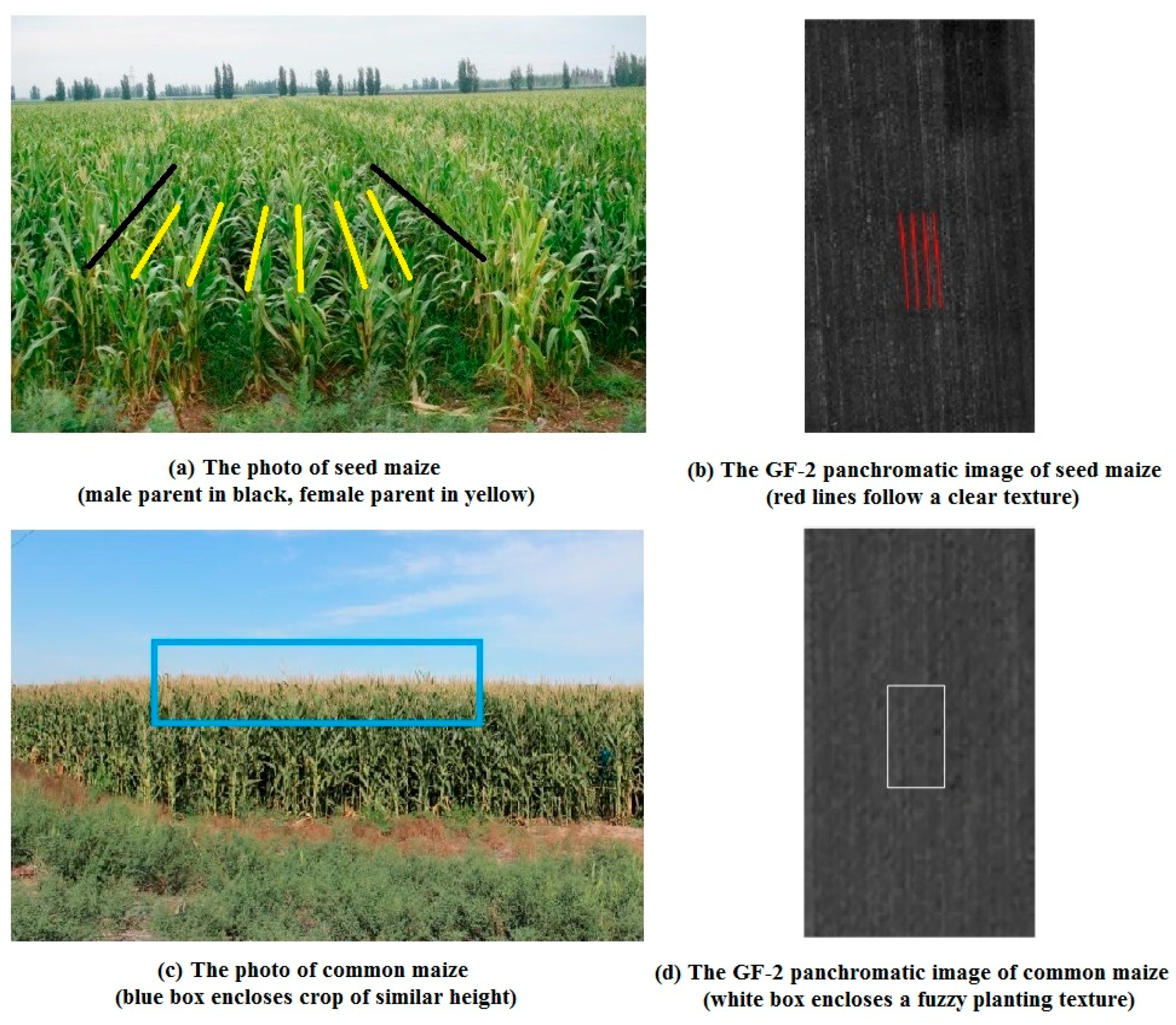
The maize seed-producing area provides us with a similar remote-sensing recognition research scenario. In addition, other crops, even common maize, are grown around the seed maize fields. Therefore, in order to accurately identify the seed maize fields in these kind of areas, it is necessary to be able to distinguish the seed maize fields from common maize, as well as maize from other crops. These differences between seed maize, common maize and other crops are mainly reflected in the spectral reflectance, texture and other information differences of plant population canopy between plots, as well as the temporal changes in different growth periods [46]. The selection of suitable classification characteristics and methods can help identify the subtle differences between different planting patterns and varieties of the same crop. Liu et al. [46] and Zhang et al. [47] respectively took remote-sensing identification of seed maize and common maize in Linze County, Gansu Province, and Qitai County, Xinjiang Autonomous Region, China, as examples to explore the classification method of decision trees using time-series spectra and high-resolution texture characteristics.

Based on the above analysis, it can be seen that vegetation index such as enhanced vegetation index (EVI), RVI, gray-level co-occurrence matrix and other texture features of high-resolution satellite remote sensing image data, as well as their temporal variation information, have the potential to identify crops with slight differences. Random forest classifier has a good tolerance for outliers and noise and is not easy to overfit, so it can be used to build a classification model for seed maize field detection.

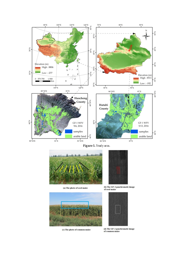
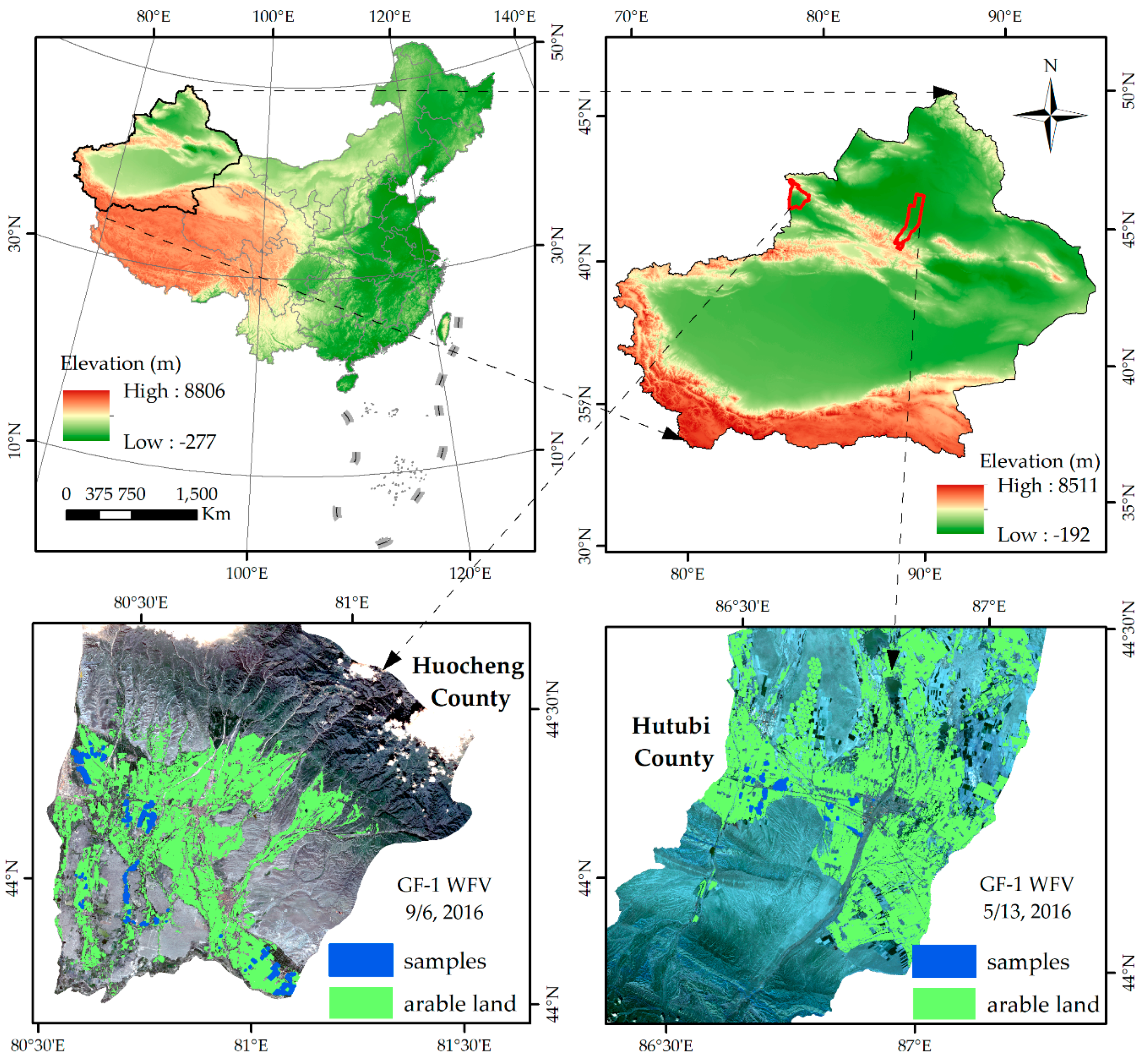
In order to explore the identification method for two kinds of planting patterns (seed and common) and variety types (inbred and hybrid) of the same crop (maize). This paper selected two maize seed production bases in Huocheng County and Hutubi County in Xinjiang Uygur Autonomous Region of China as the study area, and took Landsat 8, China Gaofen 1 satellite (GF-1) and Gaofen-2 satellite (GF-2) as the data source. Using random forest classifier, we propose a seed maize identification method that combines multi-temporal spectral features and texture features. It provides a reference for the large-scale mapping of seed maize field and fine classification of other crops by remote sensing.

2. Materials

2.1. Study Area

The study areas are Huocheng County and Hutubi County in the Xinjiang Uygur Autonomous Region, which belong to different ecological zones and are the major seed maize production areas in Xinjiang, China (Figure 1). Huocheng County is a border region of China with a geographical range of longitude 80.18–80.40E and latitude 43.65–44.83N. Agriculture is one of the mainstays of Huocheng County. There are approximately 964,500 acres of arable land in this region, which is in a temperate semi-arid climate, and it receives full sunlight throughout the year, significant temperature variations between winter and summer, and significant temperature variations between day and night. In this climate, the amount of precipitation tends to be low. The average annual precipitation and average temperature in the area are 140–460 mm and 8.2–9.4 °C, respectively. The annual sunshine hours are 2550–3500 h, and the frost-free period is 167–187 days. This area provides a good planting environment for major crops such as seed maize, common maize, rice, cotton, grapes, wheat, sugar beets and soybeans. It is also the most important planting area for seed maize in Ili Kazak Autonomous Prefecture. Hutubi County is located in the middle of the northern slope of Tianshan, Junggar Basin south rim, between 86°05′~87°07′E and 43°16′~45°20′N. The alluvial plain in the central area is the main planting area of crops in Hutubi County, which has a temperate continental climate with high variation between the four seasons. The annual average precipitation is 167 mm, the frost-free period lasts for 180 days, and the average temperatures of the coldest and hottest months are –17.1 °C and 26.4 °C, respectively. From May to August, during the season for strong crop growth in the plains, the average daily sunshine hours reach more than 10 h, and in July, they reach more than 11 h. The following categories were included in this study: cotton, seed maize, common maize, grapes, pumpkins, tomatoes, and watermelons.

2.2. Data Sources

2.2.1. Remote-Sensing Data

The data used in this study consist of a time series of GF-1 wide field view (WFV) imagery, Landsat8 OLI imagery from March to September, 2016 and GF-2 panchromatic sensor (PMS) imagery. The specific parameters are shown in

Table 1. Satellite parameters.

	Parameter	Value	Image Dates in Huocheng (Month/Day)	Image Dates in Hutubi (Month/Day)
Gaofen-1 wide field view (GF-1 WFV)	Band 1-Blue (μm)	0.45~0.52	3/9, 4/19, 5/30, 6/13, 7/10, 8/12, 9/1, 9/6,	4/19, 5/1, 5/13, 6/7, 6/24, 6/27, 7/2, 7/10, 8/3, 8/12
	Band 2-Green (μm)	0.52~0.59
	Band 3-Red (μm)	0.63~0.69
	Band 4-NIR (μm)	0.77~0.89
	Spatial resolution (m)	16
	Revisit time (day)	4
Gaofen-2 wide field view (GF-2 PMS)	Panchromatic (μm)	0.45~0.90	7/26	7/5, 7/10
	Spatial resolution (m)	1
	Revisit time (day)	5
Landsat8 Operational Land Imager (Landsat-8 OLI)	Band 2-Blue (μm)	0.45~0.51	6/20, 6/29, 9/17, 9/23
	Band 3-Green (μm)	0.52~0.60
	Band 4-Red (μm)	0.63~0.68
	Band 5-NIR (μm)	0.85~0.88
	Spatial resolution (m)	30
	Revisit time (day)	5

. The GF-1 satellite is the first satellite in China’s high-resolution Earth observation system. Since the study area is large and relatively homogeneous, Landsat8 Operational Land Imager (OLI) data with path147/row 29 were selected as a supplement. The multi-temporal GF-1 WFV and Landsat 8 OLI image series were then used to describe the changes in the spectral characteristics of the agricultural crop conditions. The GF-2 satellite is the first civil optical remote sensing satellite with spatial resolution better than 1 m that was independently developed by China and has high radiation accuracy, high positioning accuracy, and rapid posture maneuverability.

In the seed maize-producing fields, two inbred lines (as female and male parent respectively) are planted in different rows, usually every 4–8 rows of female parents have 1 row of male parent, with row spacing of 0.6–0.8m. The male parent supplies pollen to the female parent, on which hybrid seeds are harvested. This heterogeneous population structure can be reflected in the spectral reflectance and canopy texture differences in remote sensing images. Usually, the maternal tassels are removed during tasseling in mid-July, and the paternal line is cut off after pollination at the beginning of August. Thus, the stripe texture unit size in the high spatial resolution remote-sensing images is between 3.6 m and 4.8 m. This texture feature should be available at a 1 m spatial resolution in the GF-2 panchromatic images. Because of the difference in planting patterns, the texture characteristics of common maize are not noticeable. Figure 2 shows the photo and GF-2 panchromatic image acquired on 26 July 2016 of seed maize and common maize. In Figure 2, we can see texture features clearly in both the photo and GF-2 image of seed maize. Therefore, GF-2 panchromatic images from the middle of July to the beginning of August were selected to analyze the feature contours and texture features.

2.2.2. Field Sample Data

A total of 162 samples were obtained in Huocheng County from the field survey, and included rice, seed maize, cotton, grapes, wheat, sugar beets, common maize, and soybeans. These samples were polygons, with an average of 148 GF-1 WFV 16 m pixels per polygon sample, and they were primarily distributed in the southern half of the county, the primary seed maize-planting area. In Hutubi County, there are 80 samples of cotton, seed maize, grapes, pumpkins, common maize, tomatoes and watermelons. On average, each polygon sample covered 139 pixels of GF-1 WFV 16 m, and the samples were evenly distributed in the central crop planting area in the middle of the county. The attribute table of the samples includes the crop type, plot area, geographic coordinates, and crop growth period. According to the national standardized planting mode and management of seed maize, the geographical location of the field was relatively stable over a short period of time. Therefore, the arable land data from 2014 were used, which were derived from the results of the country’s annual land change survey, are in raster format, and they were the field boundary of the study area. These reference data were used for crop classification and validation.

3. Methods

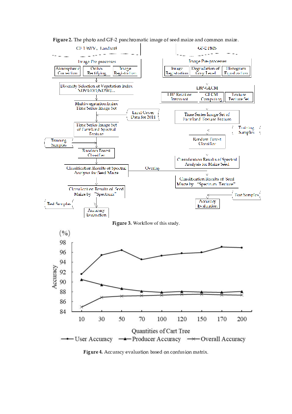
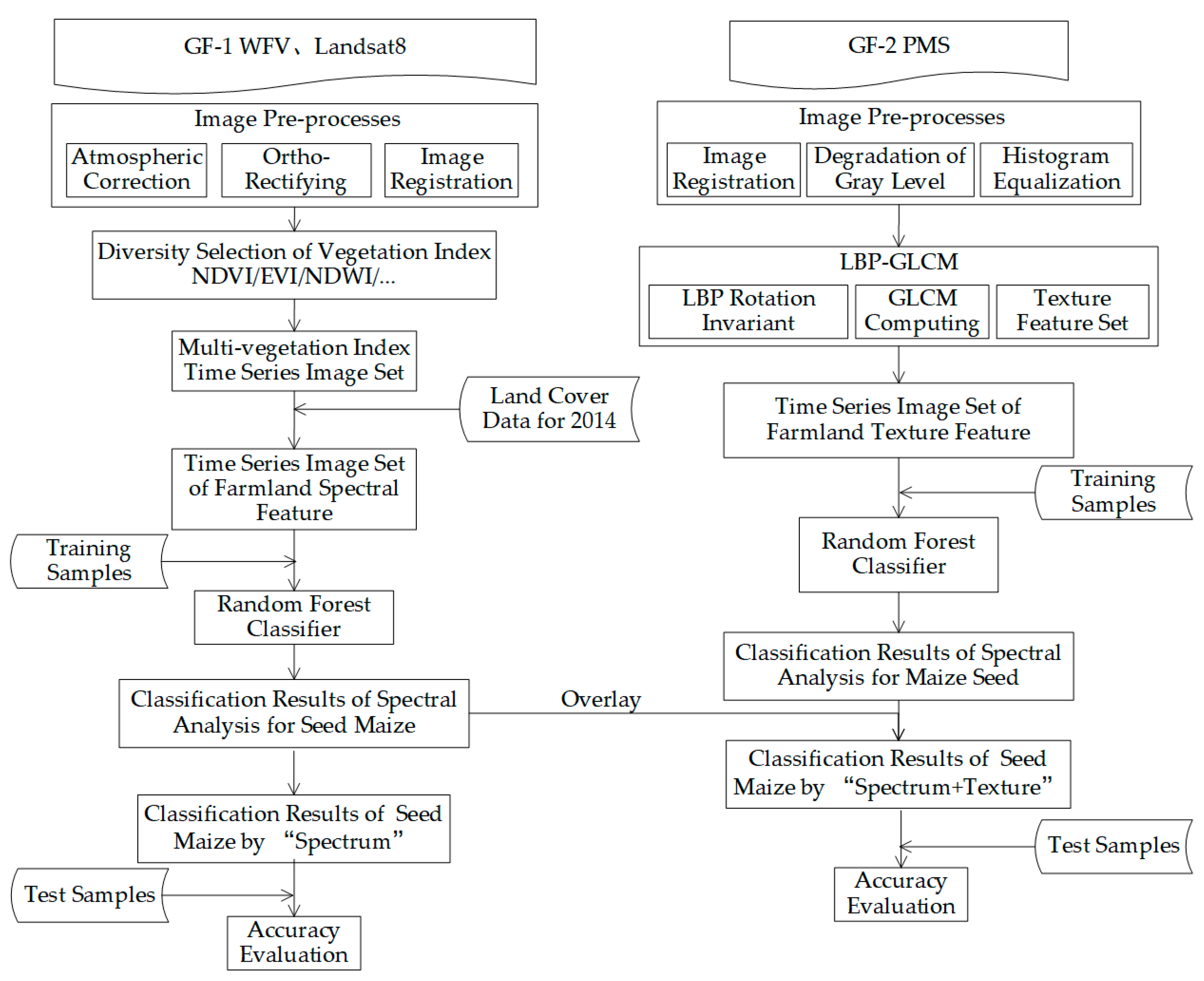
The research workflow is shown in Figure 3. It mainly includes five parts: data preprocessing, spectral feature optimization, texture feature calculation, random forest classification, and accuracy assessment. First, preprocess the remote sensing data based on the automatic processing platform developed by our team. The second step is to use the correlation coefficient to optimize the spectral characteristics. The third step is to calculate the texture features. The fourth step is to classify only the spectral features and fusion spectrum and texture features in the regions covered by GF-2 image respectively. Finally, the land cover data in 2014 were used to mask and evaluate the accuracy separately.

3.1. Data Preprocessing

Both the GF-1 images and the field samples were stored using the Raster Dataset Clean and Reconstitution Multi-Grid (RDCRMG) grid system developed by China Agricultural University [48]. Based on C # combined with the Geospatial Data Abstraction Library (GDAL), procedures such as radiometric calibration, ortho-rectification, and the image registration of their products were performed for all the data. Atmospheric correction and radiometric calibration were performed using Fast Line-of-Site Atmospheric Analysis of Spectral Hypercube (FLAASH) tools [49]. According to the mid-latitude location and the image capturing time of the study area, a suitable atmospheric model was selected. Since the urban area in the study area is relatively small, a rural aerosol model was selected to correct the effects of the aerosol factors. The GF satellite image products used in this study were provided with rational polynomial coefficient (RPC) files. In addition, the parameters provided in the RPC files were used to perform ortho-rectification on high-resolution remote sensing images. In this paper, multi-source remote sensing images and multi-temporal remote sensing images were well geo-referenced.

3.2. Spectral Feature Optimization

In this paper, a correlation coefficient calculated by Python was used to select the better VIs. Correlation coefficient is a statistical indicator designed by statistician Carl Pearson and is a measure of the degree of linear correlation between study variables. All the field survey samples were analyzed in this paper.

The VI quantifies the vegetation properties by helping transform the reflectance of two or more spectral bands [50]. Considering the differences in phenology, seasonal differences, as well as the significance and anti-saturation degree of different VIs, the commonly used VIs can be divided into four categories: (1) To reflect the comprehensive change in crop growth: normalized difference vegetation index (NDVI), enhanced vegetation index (EVI). (2) To reflect crop greenness: triangle vegetation index (TVI), ratio vegetation index (RVI), green normalized difference vegetation index (GNDVI). (3) To reflect crop soil background: difference vegetation index (DVI), soil regulation vegetation index (SAVI). (4) To reflect the canopy moisture content of crops: normalized difference water index (NDWI) [8]. The formula is in

Table 2. Vegetation indices tested in this study.

Vegetation Index (VI)	VI Adapted to GF1/L8	Implication
Normalized Difference Vegetation Index (NDVI) [8]	NDVI = (NIR − R)/(NIR + R)	Vegetation status, canopy structure
Enhance Vegetation Index (EVI) [8]	EVI = 2.5*(NIR − R)/(NIR + 6R − 7.5B + 1)	Vegetation status, canopy structure
Ratio Vegetation Index (RVI) [8]	RVI = NIR/R	Vegetation status, canopy structure, leaf pigments
Green Normalized Difference Vegetation Index (GNDVI) [51]	GNDVI = (NIR − G)/(NIR + G)	Leaf pigments, vegetation status
Triangle Vegetation Index (TVI) [8]	TVI = 60*(NIR − G) − 100*(R − G)	Leaf pigments, vegetation status
Difference Vegetation Index (DVI) [8]	DVI = NIR − R	Vegetation status, soil background
Soil-Adjusted Vegetation Index (SAVI) [51]	SAVI = (1 + L)1(NIR − R)/(NIR + R + L)	Vegetation status, soil background
Normalized Difference Water Index (NDWI) [8]	NDWI = (G − NIR)/(G + NIR)	Canopy structure, water content

as follows:

In the above formula, B, G, R, NIR are the reflectance of blue, green, red and near-infrared bands, respectively. L is the soil conditioning parameter and the value is 0.5.

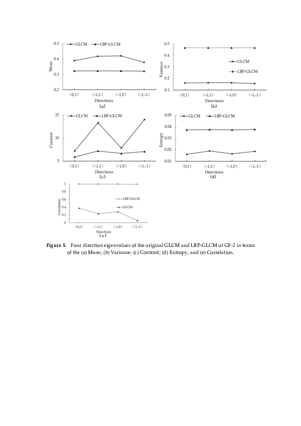
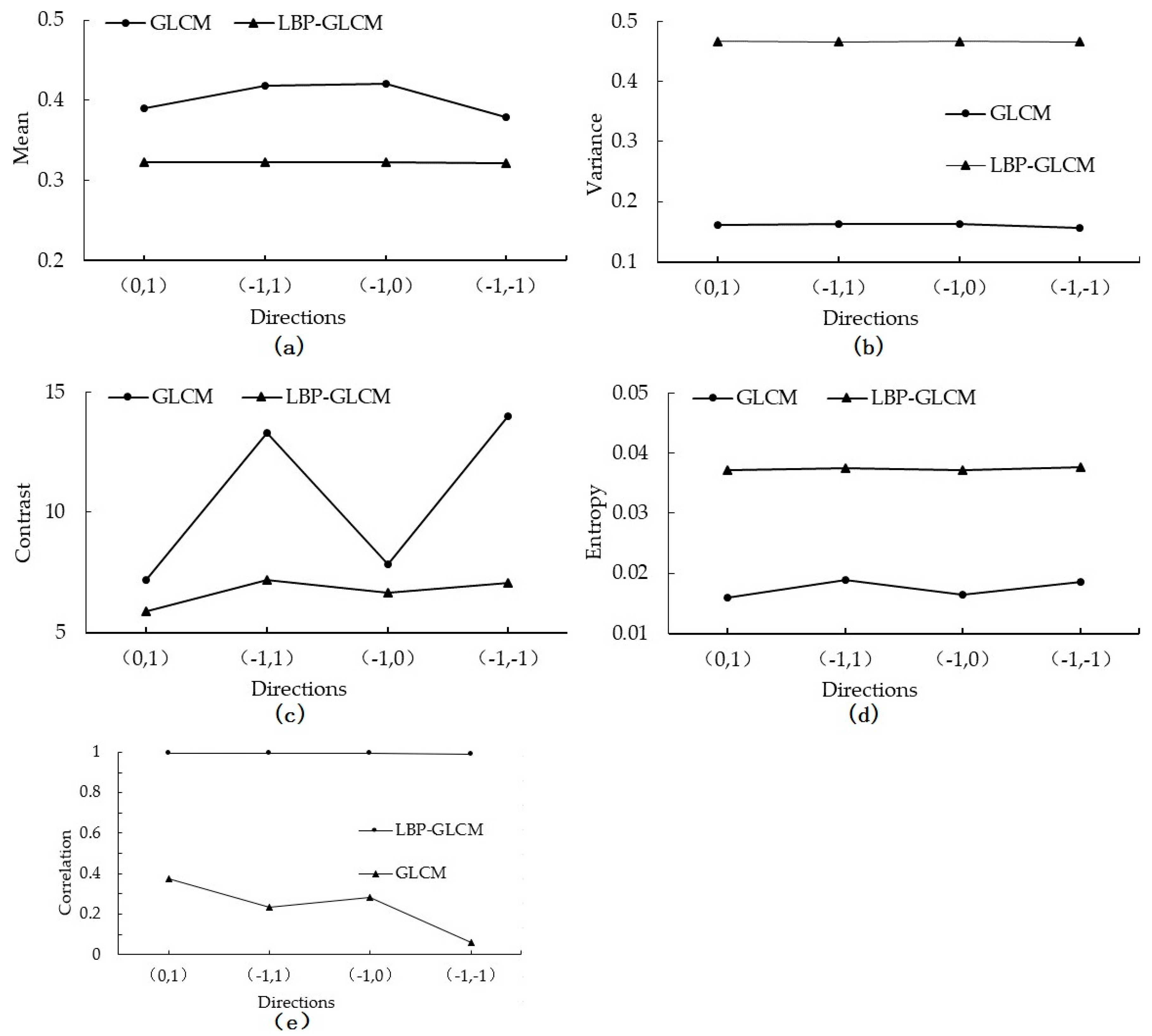
3.3. LBP-GLCM

GLCM was first proposed by Haralick [52] in 1973, which is one of the most common and widely used texture statistical analysis methods. The element values in the matrix represent the joint conditional probability density between the gray levels, which means that given the spatial distance d and the direction θ, the probability (i.e., frequency) of gray level j occurring when the gray level i is the starting point. It can calculate 14 texture features, such as angular second-order moment, entropy, contrast, and correlation. In this study, five features calculated by Python are selected for experiment, namely mean, variance, contrast, entropy, and correlation. Although the strip texture information exists on the same structure for the seed maize fields, the texture direction varies in the same remote sensing images. To eliminate the influence of the crop planting direction, before the GLCM is calculated, the image is first transformed into a local binary pattern (LBP) with rotation invariance. The LBP is an operator that is used to describe local texture features of images. It has significant advantages such as rotation invariance and gray invariance.

Specifically, the minimum and the most central pixel values in the binary pattern of 8 domains around the pixel points are taken, and the LBP image with rotation invariance is obtained. There are three extensions to the original operator to describe texture features, namely rotation invariant patterns. $LB{P}_{P,R}^{ri}$, uniform patterns $U\left(LB{P}_{P,R}\right)$, and rotation invariant uniform patterns $LB{P}_{P,R}^{riu2}$, which can be calculated using the following equation:

$$LB{P}_{P,R}^{riu2}=\left\{\begin{array}{c}{\displaystyle \sum }_{P=0}^{P-1}s\left(g_p-g_c\right),\left(U\left(LB{P}_{P,R}\right)\le 2\right)\\ P+1, \left(U\left(LB{P}_{P,R}\right)>2\right)\end{array}\right.,$$

(1)

The calculation formula for LBP uniform patterns is

$$U\left(LB{P}_{P,R}\right)=\left|s\left(g_{p-1}-g_c\right)-s\left(g_0-g_c\right)\right|+{\displaystyle \sum }_{p=1}^{p-1}\left|s\left(g_{p-1}-g_c\right)-s\left(g_0-g_c\right)\right|,$$

(2)

where $R$ is the neighborhood radius, $P$ is the number of pixels in the circular neighborhood of the LBP algorithm, the $g_c$ is the grayscale of the neighborhood center cell, and the $g_p$ is the grayscale of all the other cells except the central cell in the domain.

The threshold formula is

$$S\left(x\right)=\left\{\begin{array}{c}1, \left(x\ge 0\right)\\ 0, \left(x<0\right)\end{array}\right.,$$

(3)

where $x$ is the difference between the central pixel $g_c$ and the pixel $g_{p-1}$. Comparing the $g_{p-1}$ of P -1 gray in the circular neighborhood with the center gray $g_c$, subblocks larger than the center size are represented by 1, otherwise by 0.

3.4. Random Forest Classification

Random forest (RF) is an integrated algorithm, which belongs to the Bagging type. By combining multiple weak classifiers, the final result is obtained by voting, which gives the overall model result a higher precision and generalization ability [8].

Random forests can process high-dimensional data well, and this method has significant advantages when there are many samples and features. In this study, multi-temporal single-band VI image series were compiled into a multi-layer data cube for further analysis. In Huocheng County, 8 planting indexes were calculated for 12 scene data, so this data cube has 96 bands, and correspondingly, there are 80 bands in Hutubi County.

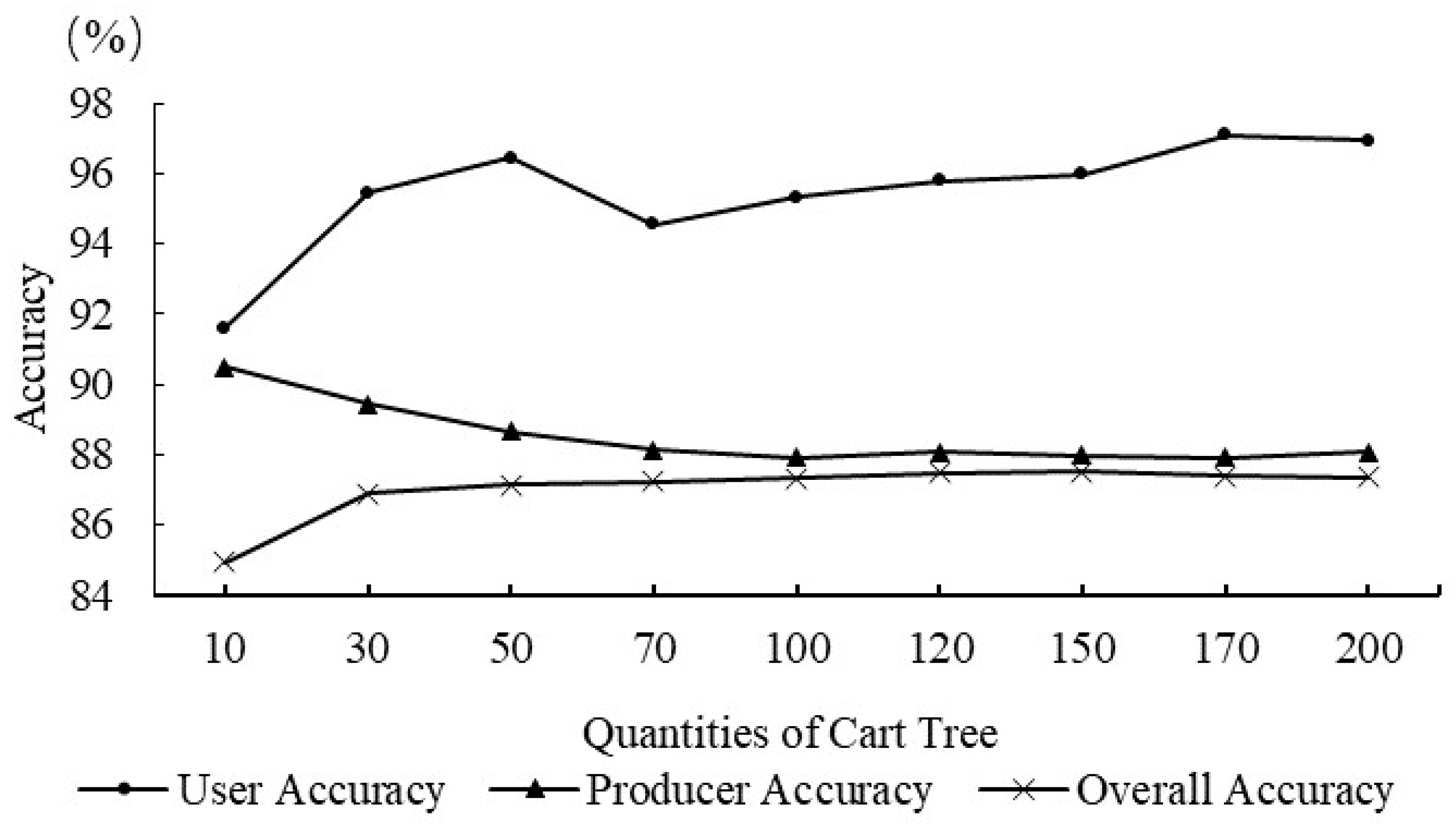
In principle, the more decision trees there are in the RF classifier, the better the prediction. However, there is a trade-off between the classification accuracy and the time efficiency. In this paper, we tested different numbers of trees, including 10, 30, 50, 70, 100, 120, 150, 170, and 200 (Figure 4), and we selected 150 trees to classify the seed maize fields when considering both the classification accuracy and time efficiency.

Crop classification based on remote sensing data is essentially based on the similarity of pixels. In this article, we combined C# with Waikato Environment for Knowledge Analysis (weka), which is an open source machine learning and data mining software based on JAVA environment, to build data sets and classification models. First of all, the characteristics of the samples were extracted from remote sensing image data. Then, the comprehensive characteristics of long phase data, generate the sample set, as the input data of RF classifier, used in the model of training. Finally, the same time-phase remote sensing data were put into the classifier to obtain the crop classification results.

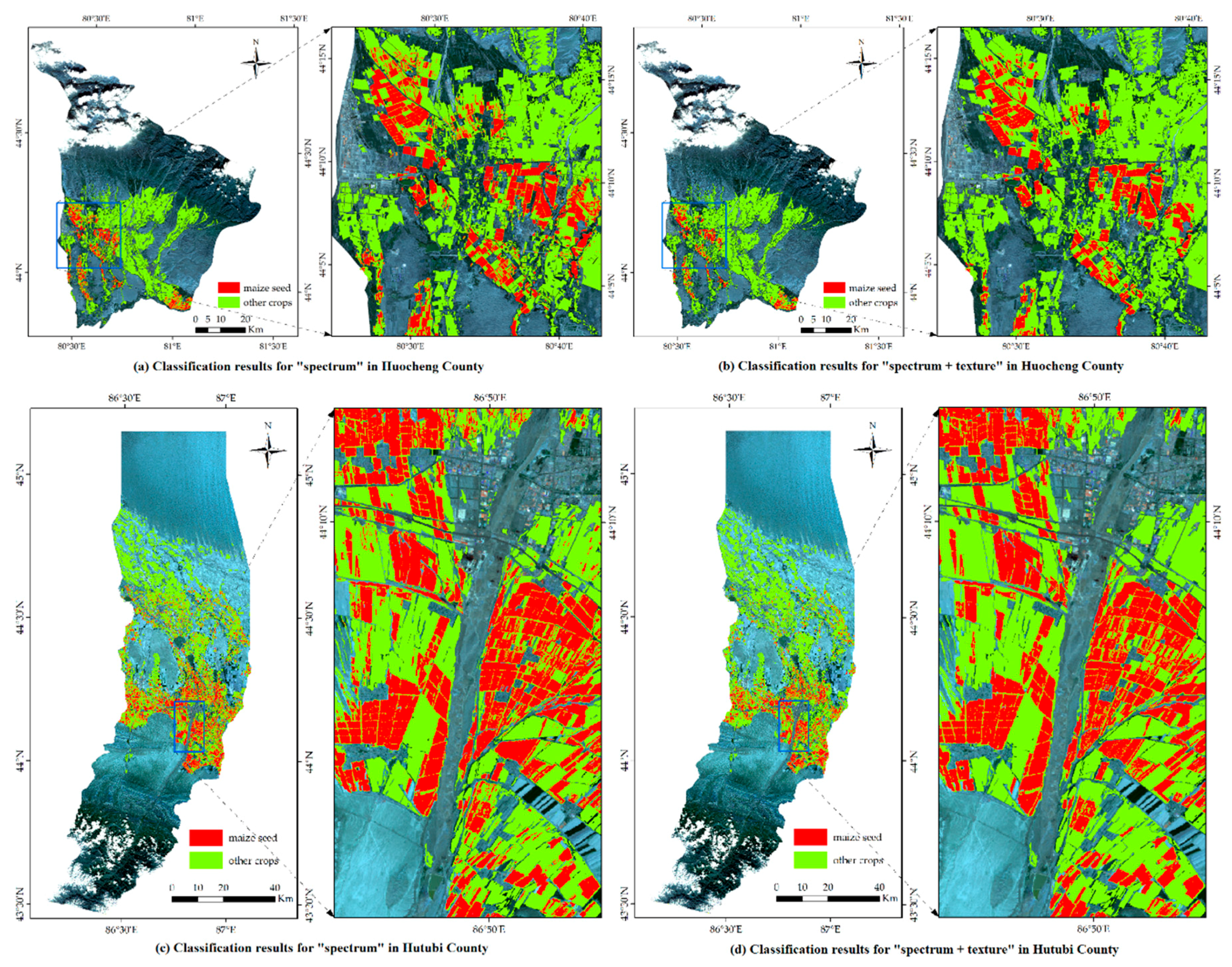
In this paper, two experiments are designed, which are based solely on spectral data and fuse spectrum and texture data. First of all, according to the phenological calendar and the planting system used for the primary crops in the study area, the vegetation index system was constructed, the multi-temporal spectral characteristics were analyzed, and the seed maize was preliminarily identified using the spectral characteristics. Then, in the regions covered by GF-2 image, the classification results were further recognized by a texture analysis of high spatial resolution remote sensing images. In this way, two classification results of seed maize can be obtained.

3.5. Accuracy Assessment

In this paper, the arable land data of 2014 were firstly used for masking, then a random selection resulting in 114 samples (70%) as training samples, with the remaining samples (30%) as verification samples, and the confusion matrix based on Python was used to assess the classification results. By constructing a confusion matrix, four accuracy assessment indexes can be obtained: overall accuracy (OA), producer accuracy (PA), user accuracy (UA), kappa coefficient (K). Kappa analysis provided a measure of the magnitude of agreement between the predicted and actual class membership [53]. A kappa value of 0 represents a total random classification, while a kappa value of 1 corresponds to a perfect agreement between the reference and classification data. The calculation formula for each indicator is as follows:

$$\mathrm{OA}=\frac{TP+TN}{N},$$

(4)

$$\mathrm{PA}=\frac{TP}{TP+FN},$$

(5)

$$\mathrm{UA}=\frac{TP}{TP+FP},$$

(6)

$$\mathrm{K}=\frac{OA-P_e}{1-P_e},$$

(7)

$$P_e=\frac{\left(TP+FN\right)\left(TP+FP\right)+\left(FP+TN\right)\left(FN+TN\right)}{N^2},$$

(8)

where TP and FN, respectively, refer to the true category of samples as positive examples, and the model prediction results as positive examples and negative examples. TN and FP refer to the negative examples of the true category of samples, which are predicted by the model as negative examples and positive examples. N is the total number of real samples.

4. Results

4.1. Feature Optimization Result

Data from Huocheng County were used to evaluate the VI correlation of seed maize and to apply the same rules to both regions. The correlation indices of VIs during different growing stages are shown in

Table 3. Correlation of VI characteristics in Huocheng County on April 19.

	NDVI	EVI	GNDVI	TVI	RVI	NDWI	SAVI	DVI
NDVI	1	0.996	0.995	0.994	0.977	−0.995	1	0.993
EVI		1	0.991	0.999	0.987	−0.991	0.996	0.999
GNDVI			1	0.987	0.968	−1	0.995	0.99
TVI				1	0.984	−0.987	0.994	0.998
RVI					1	−0.968	0.977	0.985
NDWI						1	−0.995	−0.99
SAVI							1	0.993
DVI								1

,

Table 4. Correlation of VI characteristics in Huocheng County on May 30.

	NDVI	EVI	GNDVI	TVI	RVI	NDWI	SAVI	DVI
NDVI	1	0.984	0.995	0.979	0.934	−0.995	1	0.969
EVI		1	0.979	0.998	0.95	−0.979	0.984	0.995
GNDVI			1	0.973	0.932	−1	0.995	0.966
TVI				1	0.936	−0.973	0.979	0.998
RVI					1	−0.932	0.934	0.936
NDWI						1	−0.995	−0.966
SAVI							1	0.969
DVI								1

,

Table 5. Correlation of VI characteristics in Huocheng County on June 13.

	NDVI	EVI	GNDVI	TVI	RVI	NDWI	SAVI	DVI
NDVI	1	0.909	0.986	0.841	0.928	−0.986	1	0.827
EVI		1	0.91	0.982	0.864	−0.91	0.909	0.978
GNDVI			1	0.844	0.92	−1	0.986	0.839
TVI				1	0.81	−0.844	0.841	0.999
RVI					1	−0.92	0.928	0.802
NDWI						1	−0.986	−0.839
SAVI							1	0.827
DVI								1

and

Table 6. Correlation of VI characteristics in Huocheng County on June 29.

	NDVI	EVI	GNDVI	TVI	RVI	NDWI	SAVI	DVI
NDVI	1	0.904	0.987	0.855	0.857	−0.987	1	0.815
EVI		1	0.889	0.994	0.802	−0.889	0.904	0.983
GNDVI			1	0.836	0.887	−1	0.987	0.8
TVI				1	0.756	−0.836	0.855	0.996
RVI					1	−0.887	0.857	0.727
NDWI						1	−0.987	−0.8
SAVI							1	0.815
DVI								1

. We can find that there is a high correlation among the various VIs. The lowest value was the correlation coefficient between RVI and DVI on June 29, with a value of 0.727. The correlation coefficients of vegetation index in other phases were all greater than 0.8. Among them, the largest correlation coefficients are NDVI and SAVI, NDWI and GNDVI, and their absolute correlation coefficients are all 1. Since the NDWI is quantifying different aspects of vegetation (a water-related property) from other VIs, the correlation indices between the NDWI and other VIs are negative.

Table 7. T-test result of vegetation index with absolute correlation coefficient of 1.

	19-Apr	30-May	13-Jun	29-Jun
NDVI vs. SAVI	0.12	<0.01	<0.01	<0.01
NDWI vs. GNDVI	<0.01	<0.01	<0.01	<0.01

is the T-test result of the vegetation index with an absolute correlation coefficient of 1. It can be seen from the figure that, except NDVI and SAVI with low significance on April 19, the other t-test results all show extremely significant correlations. The increase in the number of features will greatly increase the calculation dimension and reduce the calculation efficiency. So we discarded SAVI and GNDVI, the NDVI, EVI, TVI, RVI, NDWI, DVI were selected as the input data in the final classification.

4.2. Local Binary Pattern-Gray-Level Co-Occurrence Matrix (LBP-GLCM) Analysis

The GLCM in this paper is determined by using two parameters, the distance and the direction. According to the field investigation, the tassels in the female parent row are removed from the maize planting field in the study area at a specific time, while the male parent row retains its tassels. In the GF-2 panchromatic image at a 1-meter resolution, the parents of seed-producing maize had obvious gray contrast in the neighborhood. Simultaneously, because the line ratio of the parents is 1:6 and the row spacing is 60 cm, the texture structure of the seed maize field is based on approximately one pixel, so the distance parameter of the GLCM is based on one pixel. In large-scale crop planting, it is difficult to ensure the same crop planting direction.

Figure 5 shows five texture features of GLCM in the (0, 1), (−1, 1), (−1, 0), and (−1, −1) directions without LBP rotation invariant processing and five texture features after calculating the LBP invariant rotation. The texture features of GLCM in different directions are computed separately from the images transformed by rotation-invariant LBP. The variation in the quantization values for the same feature in different directions is relatively small, so it can be used as a classification feature to reflect the texture structure.

4.3. Accuracy Assessment and Analysis

The overall accuracy verification results based on the spectrum in Huocheng County and Hutubi County are shown in

Table 8. Confusion matrix based on the “spectrum” in Huocheng County.

User Classes	Ground-Truth Classes (Pixels)
	Winter Wheat	Seed Maize	Rice	Grapes	Common Maize	Cotton	Total	User Accuracy (UA, %)
Winter wheat	60	57	3	63	0	0	183	32.79
Seed maize	281	9717	75	90	33	52	10,248	94.82
Rice	0	301	2352	1	10	17	2681	87.73
Grapes	0	7	123	2160	5	0	2295	94.12
Common maize	0	596	17	25	401	0	1039	38.59
Cotton	0	519	0	0	2	171	692	24.71
Total	341	11,197	2570	2339	451	240	17,138
Producer accuracy (PA, %)	17.60	86.78	91.52	92.35	88.97	71.25		86.71

and

Table 9. Confusion matrix based the “spectrum” in Hutubi County.

User Classes	Ground-Truth Classes (Pixels)
	Water-Melons	Tom-Atoes	Seed Maize	Pump-Kins	Grapes	Common Maize	Cotton	Total	UA (%)
Water-melons	419	6	81	77	0	6	43	632	66.30
Tomatoes	0	4	11	0	0	0	0	15	26.67
Seed maize	60	44	2066	15	0	20	90	2295	90.02
Pumpkins	30	0	2	86	0	0	38	156	55.13
Grapes	15	0	30	2	292	0	26	365	80.00
Common maize	0	0	6	3	0	97	4	110	88.18
Cotton	0	26	0	19	0	0	2034	2079	97.84
Total	524	80	2196	202	292	123	2235	5652
PA (%)	79.96	5.00	94.08	42.57	100.00	78.86	91.01		88.43

. The overall accuracies are 86.71% and 88.43%, and the Kappa coefficients are 0.76 and 0.83, meeting the accuracy requirements of crop classification. The user accuracy and the producer accuracy of Huocheng County’s seed maize are 94.82% and 86.78%, respectively. These results means that other crops are rarely misclassified into seed maize, but misclassified seed maize into other crops are more common, especially the mixes of seed maize fields and common maize are more serious, with 5.32% seed maize fields are mistakenly divided into common maize. In Hutubi County, both the user accuracy and the producer accuracy are higher, 90.02% and 94.08%, respectively. This is due to the fact that there are more seed maize in Hutubi County and the plots are larger, so the pepper and salt effect is lighter. So, we can find that the average overall accuracy and the Kappa coefficient of the two counties were 87.57% and 0.80. The average user accuracy for seed maize was 92.42%, and the producer accuracy was 90.43%.

In the regions covered by GF-2, the overall accuracy verification results based on the “spectrum + texture” in Huocheng County and Hutubi County are shown in

Table 10. Confusion matrix based the “spectrum + texture” in Huocheng and Hutubi County.

Ground-Truth Classes (Pixels)
	Seed Maize	Other Crops	Total	UA (%)	Seed Maize	Other Crops	Total	UA (%)
	Huocheng County				Hutubi County
	OA: 95.90%, Kappa: 0.92				OA: 97.79%, Kappa: 0.95
Seed maize	3811	33	3844	99.14%	2162	69	2231	96.91%
Other crops	247	2737	2984	91.72%	52	3181	3233	98.39%
Total	4058	2770	6828		2214	3250	5464
PA(%)	93.91%	98.81%		95.90%	97.65%	97.88%		97.79%

. For Huocheng County, the overall accuracy and Kappa coefficient for “spectrum + texture” are higher than that of "spectrum", which are 9.19% and 0.16, respectively. The omission rate is 7.13% lower than that of the “spectrum”. For Hutubi County, the overall accuracy and Kappa coefficient based on “spectrum + texture” are 9.36% and 0.12 higher than those based on "spectrum", respectively. In addition, the user accuracy and producer accuracy of “spectrum + texture” are better, since the commission rate and the omission rate are lower than that of “spectrum”. The average overall crop accuracy and the Kappa coefficient of the two counties were improved to 96.85% and 0.94, respectively. The average user accuracy of the seed maize field was improved to 98.03% and the average producer accuracy was 95.78%. Therefore, the classification method of “spectrum + texture” can obtain higher accuracy.

A confounding matrix based on field samples is not sufficiently comprehensive to evaluate classification accuracy. It is necessary to evaluate the classification results by combining crop mapping. Figure 6 shows the seed maize distribution in the Huocheng and Hutubi County. In this Figure, a and b are based on the “spectrum” and “spectrum + texture”, respectively, in Huocheng County, c and d are that of Hutubi County. We can find that the distribution of seed maize can be obtained based on both schemes, but the classification results based on “spectrum + texture” have clearer land boundaries, this is in line with the characteristics of seed maize fields such as large plot, good contiguous property and concentrated planting. So the identification of seed maize is more accurate. At the same time, comparing Huocheng County and Hutubi County, we can find that the plot in Hutubi County is larger and more orderly, which also corresponds to the higher accuracy of Hutubi County mentioned above. Therefore, the method of fusing spectrum and texture to identify seed maize is feasible.

5. Discussion

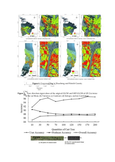
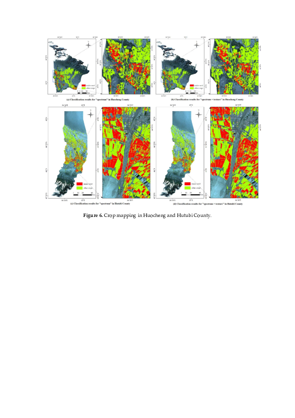
The purpose of this research was to explore the identification method for different planting patterns and varieties of the same crop. According to the differences in the planting methods and varieties of seed maize and common maize, based on Landsat 8 and GF-1 WFV multispectral sequence images, and GF-2 PMS panchromatic images with a spatial resolution of 1 m, six spectral vegetation indexes and LBP-GLCM texture features were extracted, and a random forest classification model was constructed to distinguish seed maize from common maize and other crops. The mapping accuracy of two typical seed maize producing counties was 95.90% and 97.79%, respectively. Compared with the “spectral method”, the classification accuracy was improved by 9.19 and 9.36 percentage points by adding texture features.

Another example of different planting patterns of the same crop is grazing and mowing in pastures. Grazing and mowing can cause changes in biomass and crop height, in addition, mowing can also result in soil exposure [45]. Lopes et al. [54] distinguish mowing, grazing, and mixed practices, using an object-based classification of grasslands from high-resolution satellite image time series (Formosat-2) and Gaussian mean map kernels. In a case study in Brittany, France, Dusseux et al. [55] derived the NDVI and two biophysical variables (leaf area index and fraction of vegetation cover) from a series of three SPOT images and field data to monitor pasture mowing and grazing. Compared with the above methods, the method proposed in this paper integrates texture information and spectral information to identify the two planting patterns of maize, and makes better use of the apparent differences between the two patterns. However, this study does not consider the biomass differences between seed maize and common maize. Therefore, the calculation of biomass can be used in a future study to improve the identification accuracy.

Compared with previous exploratory studies on remote-sensing identification of seed maize, the technical scheme adopted in this paper (the combination of data source, spectral feature, texture feature and classification method) has better universality. For example, the decision tree method based on multi-temporal NDVI and high-resolution texture adopted by Liu et al. [46] in the study of Linze County, Gansu Province, China, has a mapping accuracy of 83%, which is more suitable for identifying the seed-producing maize areas covered with plastic film before sowing. The decision tree method based on multi-temporal EVI and GLCM texture adopted by Zhang et al. [47] in Qitai County, Xinjiang, China, has a mapping accuracy of about 90%, but the subjective influence of artificial threshold set by the decision tree method is greater. Zhang et al. [51] adopted the random forest method based on 8 vegetation indexes and LBP-GLCM texture in Huocheng County, Xinjiang, China, with many input parameters and mapping accuracy of about 86%. In terms of texture feature extraction, the results of this study show that GF-2 panchromatic band images with 1-meter spatial resolution can also extract texture information satisfying the identification of seed production plots. Compared with the 0.3 m Geoeye-1 [46] and 0.7 m Compsat-3 [47] used in previous studies, the effective coverage of high-resolution data sources of GF-2 can be significantly improved.

Although the method presented in this paper has high accuracy in identifying seed maize, there are still some omissions and misclassification of seed maize. In the spectroscopy-based classification, the seed maize in Huocheng County had a relatively high error of omissions, and the miscounting errors of seed maize as common maize, cotton and rice were 5.32%, 4.63% and 2.69%, respectively. In Hutubi County, the misclassification error was higher. Cotton, watermelon and tomato were misclassified into seed maize, with errors of 3.92%, 2.61% and 1.92%, respectively. This is mainly because the phenological calendar and biomass of these crops are similar, and the sample size of seed maize in Huocheng County is relatively large, accounting for 65.33% of the total sample size. This unbalanced sample structure tends to increase the error of model training, making the classification results more inclined to the category with a large sample size. Therefore, in the following research, it is necessary to consider the subtle differences of these crops and explore the characteristics that are more suitable to distinguish them. At the same time, we will increase the sample sizes of fewer classes and optimize the distribution of samples, so as to make the number of samples and spatial structure more balanced.

The identification accuracy of the method in two seed maize production counties in Xinjiang is relatively high, which can be used for the statistics and mapping of annual seed maize acreage in well-known seed production areas, and the accurate estimation of seed yield based on this. However, this method requires data input from a large number of ground survey samples and full-growth season images. Therefore, it is necessary to further improve the algorithm and identification scheme for areas lacking samples and for obtaining seed production acreage in early growth season.

6. Conclusions

The aim of this paper is to explore the feasibility of high-resolution remote-sensing satellite images in identifying different planting patterns and varieties of the same crop, and expand the connotation of crop precise classification by remote sensing. The result shows that the random forest classifier constructed based on the temporal spectra and texture information extracted from high-resolution remote-sensing satellite images, combined with ground samples, can distinguish two kinds of planting patterns (seed and common) and variety types (inbred and hybrid) of maize. Moreover, the method had high precision in two representative maize seed-producing areas in Xinjiang, China, and can be used for remote-sensing mapping of large-scale maize seed-producing fields. The key findings are as follows:

By comparing and screening the vegetation indices involved in the modeling, we found that SAVI and GNDVI are redundant features for the classification of the seed maize, common maize and other crops, and only the six indices of NDVI, EVI, TVI, RVI, NDWI and DVI are required. Compared with the method using EVI as the spectral feature, the recognition accuracy was improved.

Another seed maize identification model was built based on the fusion of spectrum and texture characteristics. It was found that the texture parameters calculated based on 1-meter panchromatic band of GF-2 can also accurately express the internal differences between seed maize and common maize. There is a significant improvement in accuracy compared to using only spectral information. In addition, compared with other high-resolution images, GF-2 has a wider image width, making this method more scalable.

In this study, remote-sensing identification of seed maize was taken as an example to explore the discrimination method of different planting patterns and varieties of the same crop, which is of great reference significance for fine identification of similar crops. In addition, on this basis, the statistics and mapping of maize area for seed production can be carried out, and the growth, quality and yield of maize seeds can be calculated by combining crop nutrient, disease and yield estimation models. However, this method still has certain limitations, because it requires a large amount of sample data. Therefore, how to effectively use and improve this method in areas lacking samples is a work that needs further research.

References

1. Huang, J.; Zhuo, W.; Li, Y.; Huang, R.; Sedano, F.; Su, W.; Dong, J.; Tian, L.; Huang, Y.; Zhu, D.; et al. Comparison of three remotely sensed drought indices for assessing the impact of drought on winter wheat yield. Int. J. Digit Earth 2018, 3, 1–23. [Google Scholar] [CrossRef]
2. Zhuo, W.; Huang, J.; Li, L.; Zhang, X.; Ma, H.; Gao, X.; Huang, H.; Xu, B.; Xiao, X. Assimilating Soil Moisture Retrieved from Sentinel-1 and Sentinel-2 Data into WOFOST Model to Improve Winter Wheat Yield Estimation. Remote Sens. 2019, 11, 1618. [Google Scholar] [CrossRef] [Green Version]
3. Doraiswamy, P.C.; Hatfield, J.L.; Jackson, T.J.; Akhmedov, B.; Prueger, J.; Stern, A. Crop condition and yield simulations using Landsat and MODIS. Remote Sens. Environ. 2004, 92, 548–559. [Google Scholar] [CrossRef]
4. Huang, R.; Huang, J.; Zhang, C.; Ma, H.; Zhuo, W.; Chen, Y.; Zhu, D.; Wu, Q.; Lamin, R.M. Soil temperature estimation at different depths, using remotely sensed data. J. Integr. Agric. 2020, 19, 277–290. [Google Scholar] [CrossRef]
5. Lu, C.; Fan, L. Winter wheat yield potentials and yield gaps in the North China Plain. Field Crop. Res. 2013, 143, 98–105. [Google Scholar] [CrossRef] [Green Version]
6. Luciano, A.C.D.S.; Picoli, M.C.A.; Rocha, J.V.; Franco, H.C.J.; Sanches, G.M.; Leal, M.R.L.V.; le Maire, G. Generalized space-time classifiers for monitoring sugarcane areas in Brazil. Remote Sens. Environ. 2018, 215, 438–451. [Google Scholar] [CrossRef]
7. Yang, N.; Liu, D.; Feng, Q.; Xiong, Q.; Zhang, L.; Ren, T.; Zhao, Y.; Zhu, D.; Huang, J. Large-Scale Crop Mapping Based on Machine Learning and Parallel Computation with Grids. Remote Sens. 2019, 11, 1500. [Google Scholar] [CrossRef] [Green Version]
8. Zhang, L.; Liu, Z.; Liu, D.; Xiong, Q.; Yang, N.; Ren, T.; Zhang, C.; Zhang, X.; Li, S. Crop Mapping Based on Historical Samples and New Training Samples Generation in Heilongjiang Province, China. Sustainability 2019, 11, 5052. [Google Scholar] [CrossRef] [Green Version]
9. Peña-Barragán, J.M.; Ngugi, M.K.; Plant, R.E.; Six, J. Object-based crop identification using multiple vegetation indices, textural features and crop phenology. Remote Sens. Environ. 2011, 115, 1301–1316. [Google Scholar] [CrossRef]
10. Li, Y.; Zhu, Y.; Dai, T.; Tian, Y.; Cao, W. Quantitative relationships between leaf area index and canopy reflectance spectra of wheat. Chin. J. Appl. Ecol. 2006, 17, 1443–1447. [Google Scholar]
11. Su, X.; Geng, J.; Ma, R.; Wang, H.; Wang, X. Mangrove species classification based on multiple vegetation index extraction and joint sparse representation. Mar. Environ. Sci. 2017, 36, 114–120. [Google Scholar]
12. Jakubauskas, M.E.; Legates, D.R.; Kastens, J.H. Crop identification using harmonic analysis of time-series AVHRR NDVI data. Comput. Electron. Agr. 2002, 37, 127–139. [Google Scholar] [CrossRef]
13. Young, S.S.; Wang, C.Y. Land-cover change analysis of China using global-scale Pathfinder AVHRR Landcover (PAL) data, 1982–1992. Int. J. Remote Sens. 2001, 22, 1457–1477. [Google Scholar]
14. Running, S.W.; Loveland, T.R.; Pierce, L.L.; Nemani, R.R.; Hunt, E.R. A remote sensing based vegetation classification logic for global land cover analysis. Remote Sens. Environ. 1995, 51, 39–48. [Google Scholar] [CrossRef]
15. Geerken, R.; Zaitchik, B.; Evans, J.P. Classifying rangeland vegetation type and coverage from NDVI time series using Fourier Filtered Cycle Similarity. Int. J. Remote Sens. 2005, 26, 5535–5554. [Google Scholar] [CrossRef]
16. Badhwar, G.D. Classification of corn and soybeans using multitemporal thematic mapper data. Remote Sens. Environ. 1984, 16, 175–181. [Google Scholar] [CrossRef]
17. Richards, J.A. Thematic mapping from multitemporal image data using the principal components transformation. Remote Sens. Environ. 1984, 16, 35–46. [Google Scholar] [CrossRef]
18. Jing, X. Crop classification based on temporal and spectral information. Master’s Thesis, Xi’an University of Science and Technology, Xi’an, China, 2005. [Google Scholar]
19. Ma, L.; Xu, X.; Jia, J.; Huang, W.; Liu, L.; Cheng, Y. Crop classification method using multi-temporal TM images. Trans. Chin. Soc. Agric. Eng. 2008, 24, 191–195. [Google Scholar]
20. Liu, J.; Wang, L.; Yang, F.; Yang, L.; Wang, X. Remote sensing estimation of crop planting area based on HJ time-series images. Trans. Chin. Soc. Agric. Eng. 2015, 31, 199–206. [Google Scholar]
21. Miao, C.; Jiang, N.; Peng, S.; Lv, H.; Li, Y.; Zhang, Y.; Wang, N.; Li, J. Extraction of Paddy Land Area Based on NDVI Time-series Data: Taking Jiangsu Province as an Example. J. Geo-Inf. Sci. 2011, 13, 273–280. [Google Scholar] [CrossRef]
22. Zhang, J.; Cheng, Y.; Zhang, F.; Yue, D.; Guo, X.; Dong, H.; Wang, J.; Tang, H. Crops planting information extraction based on multi-temporal remote sensing images. Trans. Chin. Soc. Agric. Eng. 2012, 28, 134–141. [Google Scholar]
23. Hao, W.; Mei, X.; Cai, X.; Du, J.; Liu, Q. Crop planting extraction based on multi-temporal remote sensing data in Northeast China. Trans. Chin. Soc. Agric. Eng. 2011, 27, 201–207. [Google Scholar]
24. Huang, J.; Hou, Y.; Su, W.; Liu, J.; Zhu, D. Mapping corn and soybean cropped area with GF-1 WFV data. Trans. Chin. Soc. Agric. Eng. 2017, 33, 164–170. [Google Scholar]
25. Wang, L.; Liu, J.; Yang, L.; Yang, F.; Fu, C. Impact of short infrared wave band on identification accuracy of corn and soybean area. Trans. Chin. Soc. Agric. Eng. 2016, 32, 169–178. [Google Scholar]
26. Wang, L.; Liu, J.; Yang, L.; Yang, F.; Fu, C. Application of Random Forest Method in Maize-soybean Accurate Identification. Acta Agron. Sin. 2018, 44, 569. [Google Scholar] [CrossRef]
27. Zhong, L.; Gong, P.; Biging, G.S. Efficient corn and soybean mapping with temporal extendability: A multi-year experiment using Landsat imagery. Remote Sens. Environ. 2014, 140, 1–13. [Google Scholar] [CrossRef]
28. Lu, D.; Weng, Q. A survey of image classification methods and techniques for improving classification performance. Int. J. Remote Sens. 2007, 28, 823–870. [Google Scholar] [CrossRef]
29. Wang, D.; Lin, H.; Chen, J.; Zhang, Y.; Zeng, Q. Application of multi-temporal ENVISAT ASAR data to agricultural area mapping in the Pearl River Delta. Int. J. Remote Sens. 2010, 31, 1555–1572. [Google Scholar] [CrossRef]
30. Drotár, P.; Gazda, J.; Smékal, Z. An experimental comparison of feature selection methods on two-class biomedical datasets. Comput. Biol. Med. 2015, 66, 1–10. [Google Scholar] [CrossRef]
31. Wang, N.; Li, Q.; Du, X.; Zhang, Y.; Zhao, L.; Wang, H. Identification of main crops based on the univariate feature selection in Subei. J. Remote Sens. 2017, 21, 519–530. [Google Scholar]
32. Brown, J.C.; Kastens, J.H.; Coutinho, A.C.; Victoria, D.D.C.; Bishop, C.R. Classifying multiyear agricultural land use data from Mato Grosso using time-series MODIS vegetation index data. Remote Sens. Environ. 2013, 130, 39–50. [Google Scholar] [CrossRef] [Green Version]
33. Bai, X.; Wang, K.; Wang, H. Research on the classification of wood texture based on Gray Level Co-occurrence Matrix. J. Harbin Inst. Technol. 2005, 12, 1667–1670. [Google Scholar]
34. Gong, Z.; Jayas, D.S.; Deyun, J. Grain Classification with Combined Texture Model. Trans. Chin. Soc. Agric. Eng. 2001, 17, 149–153. [Google Scholar]
35. Cao, J.; Wang, Y.; Mao, W.; Zhang, X. Weed Detection Method in Wheat Field Based on Texture and Position Features. Trans. Chin. Soc. Agric. Mach. 2007, 38, 107–110. [Google Scholar]
36. Ojala, T.; Pietikainen, M.; Maenpaa, T. Multiresolution gray-scale and rotation invariant texture classification with local binary patterns. IEEE T. Pattern Anal. 2002, 24, 971–987. [Google Scholar] [CrossRef]
37. Wu, L.; Ma, X.; Qi, L.; Tan, Y.; Kuang, J.; Liang, Z. A method of target detection for crop disease spots by improved hough transform. Trans. Chin. Soc. Agric. Eng. 2014, 30, 152–159. [Google Scholar]
38. Majumdar, S.; Jayas, D.S. Classification of cereal grains using machine vision: III. Texture models. Trans. ASAE 2000, 43, 1681–1687. [Google Scholar] [CrossRef]
39. Breiman, L. Random forests. Mach. Learn. 2001, 45, 5–32. [Google Scholar] [CrossRef] [Green Version]
40. Fang, K.; Wu, J.; Zhu, J.; Xie, B. A Review of Technologies on Random Forests. Stat. Inf. Forum 2011, 26, 32–38. [Google Scholar]
41. Ghosh, A.; Sharma, R.; Joshi, P.K. Random forest classification of urban landscape using Landsat archive and ancillary data: Combining seasonal maps with decision level fusion. Appl. Geogr. 2014, 48, 31–41. [Google Scholar] [CrossRef]
42. Liu, Y.; Du, P.; Zheng, H.; Xia, J.; Liu, S. Classification of China small satellite remote sensing image based on random forests. Sci. Surv. Mapp. 2012, 37, 194–196. [Google Scholar]
43. Hao, P.; Zhan, Y.; Wang, L.; Niu, Z.; Shakir, M. Feature Selection of Time Series MODIS Data for Early Crop Classification Using Random Forest: A Case Study in Kansas, USA. Remote Sens. 2015, 7, 5347–5369. [Google Scholar] [CrossRef] [Green Version]
44. Tatsumi, K.; Yamashiki, Y.; Morante, A.K.M.; Fernandes, L.R.; Nalvarte, R.A. Pixel-based crop classification in Peru from Landsat 7 ETM+ images using a Random Forest model. J. Agric. Meteorol. 2016, 72, 1–11. [Google Scholar] [CrossRef] [Green Version]
45. Bégué, A.; Arvor, D.; Bellon, B.; Betbeder, J.; de Abelleyra, D.; PD Ferraz, R.; Lebourgeois, V.; Lelong, C.; Simões, M.; Verón, S.R. Remote Sensing and Cropping Practices: A Review. Remote Sens. 2018, 10, 99. [Google Scholar] [CrossRef] [Green Version]
46. Liu, Z.; Li, Z.; Zhang, Y.; Zhang, C.; Huang, J.; Zhu, D. Seed Maize Identification Based on Time-series EVI Decision Tree Classification and High Resolution Remote Sensing Texture Analysis. Trans. Chin. Soc. Agric. Mach. 2015, 46, 321–327. [Google Scholar]
47. Zhang, C.; Qiao, M.; Liu, Z.; Jin, H.; Ning, M.; Sun, H. Texture scale analysis and identification of seed maize fields based on UAV and satellite remote sensing. Trans. Chin. Soc. Agric. Eng. 2017, 33, 98–104. [Google Scholar]
48. Ye, S.; Liu, D.; Yao, X.; Tang, H.; Xiong, Q.; Zhuo, W.; Du, Z.; Huang, J.; Su, W.; Shen, S.; et al. RDCRMG: A Raster Dataset Clean & Reconstitution Multi-Grid Architecture for Remote Sensing Monitoring of Vegetation Dryness. Remote Sens. 2018, 10, 1376. [Google Scholar]
49. Matthew, M.W.; Adler-Golden, S.M.; Berk, A.; Richtsmeier, S.C.; Levine, R.Y.; Bernstein, L.S.; Acharya, P.K.; Anderson, G.P.; Felde, G.W.; Hoke, M.L.; et al. Status of atmospheric correction using a MODTRAN4-based algorithm. In Proceedings of the Conference on Algorithms for Multispectral, Hyperspectral, and Ultraspectral Imagery VI, Orlando, FL, USA, 24–26 April 2000; pp. 199–207. [Google Scholar]
50. Jiang, H.; Yang, H.; Chen, X.; Wang, S.; Li, X.; Liu, K.; Cen, Y. Research on Accuracy and Stability of Inversing Vegetation Chlorophyll Content by Spectral Index Method. Spectrosc. Spect. Anal. 2015, 35, 975–981. [Google Scholar]
51. Zhang, C.; Qiao, M.; Liu, Z.; Liu, D.; Jin, H.; Zhu, D. Seed Maize Field Identification Based on Analysis of Remote Sensing Timing Spectrum and High Resolution Texture. Trans. Chin. Soc. Agric. Mach. 2018, 49, 218–225. [Google Scholar]
52. Haralick, R.M. Statistical and structural approaches to texture. Proc. IEEE 1979, 67, 786–804. [Google Scholar] [CrossRef]
53. Cao, X.; Li, Q.; Du, X.; Zhang, M.; Zheng, X. Exploring effect of segmentation scale on orient-based crop identification using HJ CCD data in Northeast China. IOP Conf. Ser. Earth Environ. Sci. 2014, 17, 12047. [Google Scholar] [CrossRef]
54. Lopes, M.; Fauvel, M.; Ouin, A.; Girard, S. Spectro-Temporal Heterogeneity Measures from Dense High Spatial Resolution Satellite Image Time Series: Application to Grassland Species Diversity Estimation. Remote Sens. 2017, 9, 993. [Google Scholar] [CrossRef] [Green Version]
55. Dusseux, P.; Gong, X.; Hubert-Moy, L.; Corpetti, T. Identification of grassland management practices from leaf area index time series. J. Appl. Remote Sens. 2014, 8, 083559. [Google Scholar] [CrossRef]
Figure 1. Study area.
Remotesensing 12 00362 g001
Figure 2. The photo and GF-2 panchromatic image of seed maize and common maize, among them (a) and (c) are the photo of seed maize and common maize; (b) and (d) are the GF-2 panchromatic of seed maize and common maize.
Remotesensing 12 00362 g002
Figure 3. Workflow of this study.
Remotesensing 12 00362 g003
Figure 4. Accuracy evaluation based on confusion matrix.
Remotesensing 12 00362 g004
Figure 5. Four direction eigenvalues of the original gray-level co-occurrence matrix (GLCM) and local binary pattern (LBP)-GLCM of GF-2 in terms of the (a) mean; (b) variance; (c) contrast; (d) entropy; and (e) correlation.
Remotesensing 12 00362 g005
Figure 6. Seed maize distribution in Huocheng and Hutubi County.
Remotesensing 12 00362 g006