On the Performances of Trend and Change-Point Detection Methods for Remote Sensing Data


1
Department of Statistics, Computer Science and Mathematics, Public University of Navarre, 31006 Pamplona, Spain
2
Institute of Advanced Materials and Mathematics (InaMat2), Public University of Navarre, 31006 Pamplona, Spain
3
Department of Mathematics, UNED Pamplona, 31006 Pamplona, Spain
*
Author to whom correspondence should be addressed.
Remote Sens. 2020, 12(6), 1008; https://0-doi-org.brum.beds.ac.uk/10.3390/rs12061008
Submission received: 11 February 2020
/
Revised: 6 March 2020
/
Accepted: 17 March 2020
/
Published: 21 March 2020
Abstract
:Detecting change-points and trends are common tasks in the analysis of remote sensing data. Over the years, many different methods have been proposed for those purposes, including (modified) Mann–Kendall and Cox–Stuart tests for detecting trends; and Pettitt, Buishand range, Buishand U, standard normal homogeneity (Snh), Meanvar, structure change (Strucchange), breaks for additive season and trend (BFAST), and hierarchical divisive (E.divisive) for detecting change-points. In this paper, we describe a simulation study based on including different artificial, abrupt changes at different time-periods of image time series to assess the performances of such methods. The power of the test, type I error probability, and mean absolute error (MAE) were used as performance criteria, although MAE was only calculated for change-point detection methods. The study reveals that if the magnitude of change (or trend slope) is high, and/or the change does not occur in the first or last time-periods, the methods generally have a high power and a low MAE. However, in the presence of temporal autocorrelation, MAE raises, and the probability of introducing false positives increases noticeably. The modified versions of the Mann–Kendall method for autocorrelated data reduce/moderate its type I error probability, but this reduction comes with an important power diminution. In conclusion, taking a trade-off between the power of the test and type I error probability, we conclude that the original Mann–Kendall test is generally the preferable choice. Although Mann–Kendall is not able to identify the time-period of abrupt changes, it is more reliable than other methods when detecting the existence of such changes. Finally, we look for trend/change-points in land surface temperature (LST), day and night, via monthly MODIS images in Navarre, Spain, from January 2001 to December 2018.
1. Introduction
Time-ordered satellite images are a sequence of remote sensing data during a period of time over a region of interest. The behaviour of such time-ordered data might face distributional changes over time due to external events or internal systematic changes [1,2]. Change-point and trend detection are both long-lived research questions that have been frequently raised in statistical and non-statistical communities for decades. A change-point is usually related to an abrupt or structural change in the distributional properties of data, whereas trend detection is an analysis that looks for the existence of gradual departure of data from its past [3].
Over the last few decades, many different methods have been developed to detect trend and change-points due to their important roles in model fitting and the prediction of time-ordered datasets [4,5,6,7,8,9,10,11,12]. The Mann–Kendall [13,14] and the Cox–Stuart methods [15] have been the most used non-parametric tests for trend detection. There are also other methods, based on different techniques, for detecting distributional changes in mean and/or variance. For instance, the non-parametric Pettitt’s test [16] inspired in the Mann–Whitney two sample test, and the non-parametric hierarchical E.divisive method, which identifies change-points with a divergence measure [17]. Among parametric methods, with the assumption that data are generated from a normal distribution, the Buishand range [18], Buishand U [19], standard normal homogeneity (Snh) [20], and a log-likelihood-based method search for changes in mean, variance, and multiple parameters [21,22,23,24]. In the case of multiple parameters, typically used when looking for changes in both mean and variance jointly (Meanvar), other distributions such as exponential, gamma, and Poisson may also be assumed [24]. Piecewise linear regression models are also proposed to detect changes in the coefficients of a linear regression model [25,26,27]. The method BFAST [27] decomposes the time series into trend, seasonal, and remainder components for detecting changes in both trend and seasonal components separately [28,29]. The aforesaid methods generally show a fairly high probability of detecting trend/change-points. However, in the presence of temporal autocorrelation, they show a high probability of introducing false trend/change-points [30,31,32,33,34,35]. Yet this probability, called type I error probability, varies among methods. This drawback is more noticeable in satellite imagery, wherein the temporal dependence is frequently present among consecutive time-periods. Based upon the Mann–Kendall method, several techniques are also proposed for trend detection when dealing with temporally autocorrelated data [30,31,32,33,34]. The aim of these proposals is to reduce the type I error probability of Mann–Kendall in the presence of autocorrelation, but this reduction comes with an important power diminution.
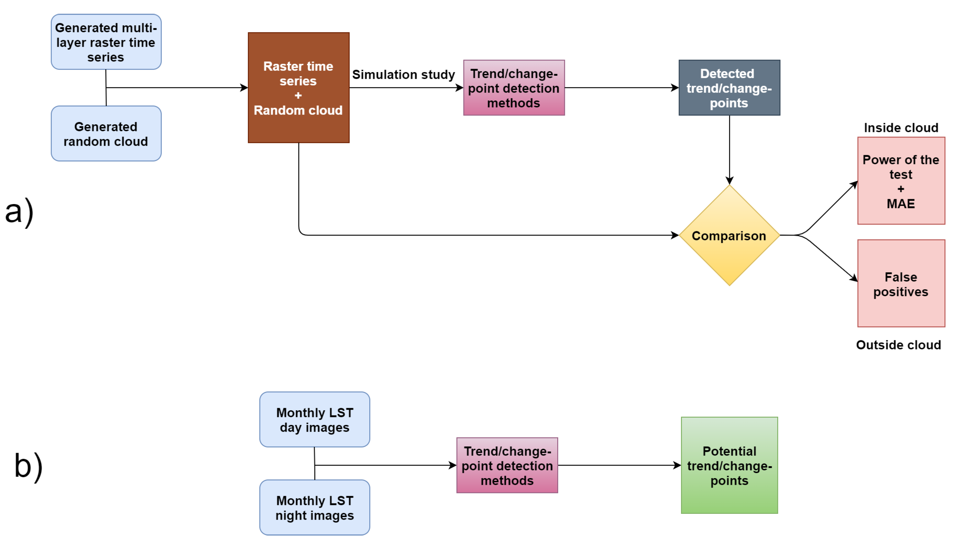
Motivated by these facts, in this paper we first provide a brief summary of the previously-mentioned trend and change-point detection methods. We then sketch out a simulation study to assess the performances of such methods, according to which we use simulated multi-layer raster time series in the absence and presence of temporal autocorrelation. We produce artificial abrupt changes at different time-periods and of different magnitudes in a randomly selected cloud; i.e., a set of joint pixels. The performances of the different methods are then assessed with the power of the test, the mean absolute error (MAE), and the type I error probability. The MAE is only calculated for the change-point detection methods, since trend detection methods are only able detect the existence of abrupt changes and not the time-period that such a change occurs in. The methods with better performances are also used to study the monthly remote sensing LST data of Navarre, Spain, from version-6 MOD11A2 product of the Moderate Resolution Imaging Spectroradiometer (MODIS) [36], from the period January 2001 to December 2018. Figure 1 shows the flowchart of the workflow of the simulation study (panel a) and the real data analysis (panel b).
The rest of the paper is organised as follows. Section 2 provides a brief summary of several trend and change-point detection methods. An example showing that abrupt changes might also provoke a monotonic trend is included. Section 3 is devoted to describing a simulation study with which to evaluate the performances of different methods in the absence and presence of temporal autocorrelation. In Section 4 we look for trend/change-points in the remote sensing LST data of Navarre, Spain. The paper ends with the conclusions and discussion in Section 5.
2. Trend and Change-Point Detection
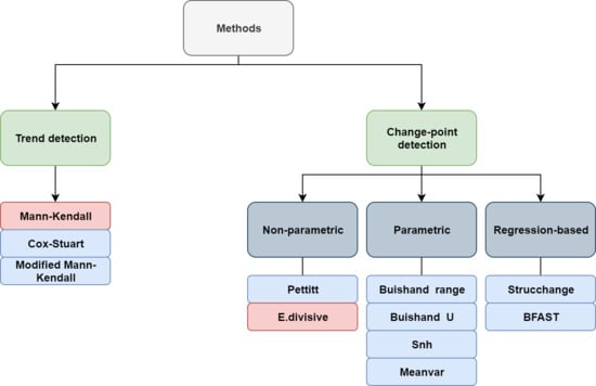
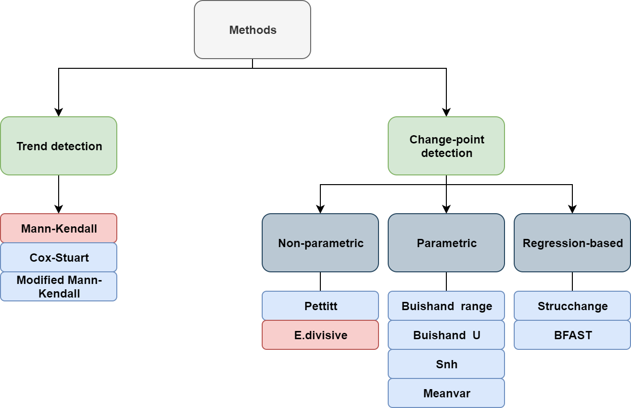
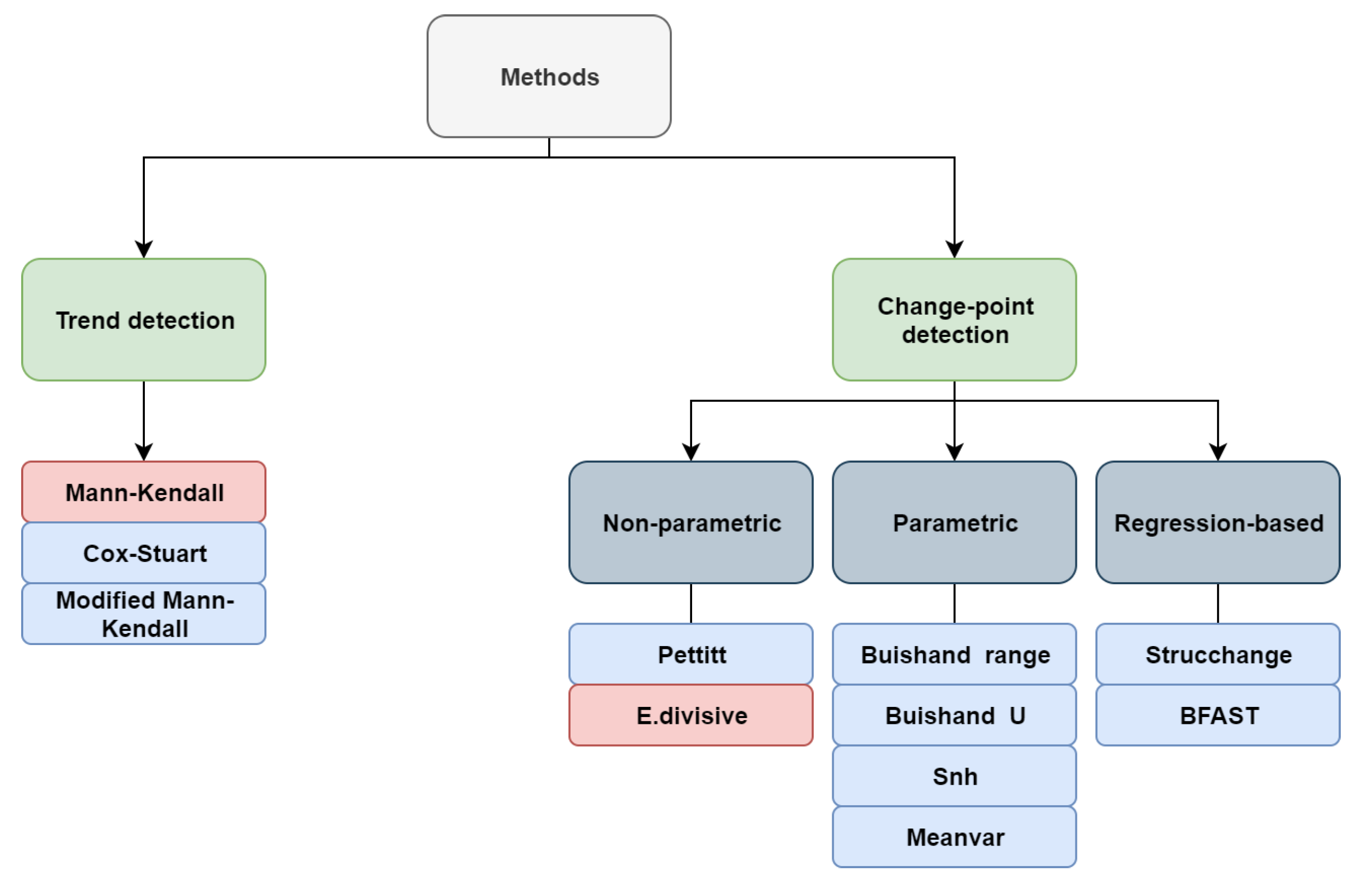
When studying time-ordered observations, it might be of interest to look for gradual and/or abrupt changes in the distribution of data over time. The process of identifying an abrupt change, usually due to distributional or structural change, is called change-point detection, in which a change-point refers to a time-period in which the behaviour of observations somehow changes. Gradual changes are, however, considered as smooth departures from past norms [3,37]. Detecting trend and change-points is generally considered for time series data, and then, it can also be used in time-ordered satellite images to look for possible locations where the behaviour of data has changed at some time. Figure 2 shows a diagram that classifies the methods we consider in this paper. They are divided into two general groups: trend and change-point detection methods. Further, we classify change-point methods into three sub-groups: non-parametric methods, which are those with no assumption about the data distribution; parametric methods, which assume that data comes from a particular distribution; and regression-based methods, which look for changes in the coefficients of a linear regression model. Modified Mann–Kendall refers to several techniques considering different modifications for the original Mann–Kendall test to deal with autocorrelated data [30,31,32,33,34].
Throughout the paper, we denote a sequence of time-ordered observations as , . We next provide a brief summary of the trend and change-point detection methods considered in this article.
2.1. Trend Detection Methods
Trend detection methods generally test the null hypothesis —where data are independently and randomly ordered so that there is no particular trend in data—against the alternative hypothesis of a monotonic trend in data existing.
2.1.1. Mann–Kendall
The test statistic of Mann–Kendall trend test is of the form
where
The test statistic is asymptotically normally distributed, and under the null hypothesis it has expectation and variance when there are no ties in data [13,14]. Having no ties in data, the well-known Kendall’s is also calculated as , which is a measure of rank correlation. For small n, the use of the standardised test statistic is common, since it provides a good approximation to the normal distribution [38,39]. The approximate p-value of such a test is then calculated as
The p-value will be then compared to a pre-selected significance level . If we accept the existence of a trend in . Looking closer to (1) we see that this test actually compares each data point to all data points appeared at a later time. Thus, for instance, when the sequence shows an upward trend, the test statistic (1) has a larger value (and consequently a smaller p-value) compared to a situation wherein data points are randomly and independently ordered. Moreover, a positive value of means that data points increase with time, whereas a negative value of indicates that decrease over time. The Mann–Kendall trend test has been the most common method for trend detection hitherto, and it is widely used in the literature. In addition, there is a multivariate version of Mann–Kendall that can be applied to several sets of time-ordered data of the same size at once [39,40,41]. This, however, only indicates whether there is at least one set with trend that can dominate the others, without identifying where the dominance occurs.
According to the literature, the performance of Mann–Kendall method is affected by the presence of autocorrelation, so its type I error probability increases noticeably. To overcome this issue, several modifications have been proposed, such as pre-whitening techniques [31,32,34,42] and variance correction approaches [30,33]. Considering such modifications, the type I error probability of the Mann–Kendall method reduces significantly. For details of these techniques, we refer the interested readers to the corresponding references.
2.1.2. Cox–Stuart
The Cox–Stuart test [15] is a non-parametric sign test for detecting a trend in independent, time-ordered data. The test statistic is given by
where denotes the maximum number of signs computed as follows.
in which is the smallest integer larger than , and is the Dirac measure. This test statistic is in fact based on a paired comparison between the first and last third of data. The test statistic (3) follows, asymptotically, a normal distribution, and it is known to have lower power than the Mann–Kendall test.
2.2. Change-Point Detection Methods
Assume a situation where there is a single change-point in . Change-point detection methods basically look for a possible time such that where and are the distributions of and respectively. In this case, the null hypothesis claims that the distribution of does not change over time, while the alternative hypothesis assumes that there is a change in the distribution of at time k. We next review some of the most used change-point detection methods.
2.2.1. Pettitt’s Test
The Pettitt’s test is a non-parametric sign test based on the Mann–Whitney two sample test (rank based) [16], and its test statistic is of the form
Under the null hypothesis and for each k, the distribution of is symmetric around zero with . It is expected to have large values for when there is a shift in data. Considering continuous observations, we then have
where is the corresponding rank of data point . The approximate p-value of the Pettitt’s test is
and the value of k provided by (4) is considered the most probable change-point [16].
2.2.2. Buishand Tests
The Buishand tests assume that comes from a normal distribution with average and a known variance . Assuming a change in the mean at time k, we can then write
where is a zero-mean normal distributed variable, and is the magnitude that shifts the average of data after time k. In other words, Buishand tests assume that there is a jump in the mean of data from time k onward. There are two types of such tests: Buishand Range and Buishand U. The test statistic of Buishand range is
where
and is the average of [18]. The test statistic of Buishand U test is
The corresponding p-values of both tests are calculated using a Monte Carlo simulation. See [18,19] for more details.
2.2.3. Standard Normal Homogeneity Test (Snh)
Similarly to Buishand tests, Snh test also assumes that is generated from a normal distribution. Here, the test statistic is given by
where
and and are the average and the standard deviation of , respectively. The p-value is also calculated using a Monte Carlo simulation. The k given as a solution of (8) is considered the most probable change-point. Note that having a change at time k means that the two variables and in (9) follow normal distributions with different means [20].
2.2.4. Identifying Changes Using Both Mean and Variance Jointly (Meanvar)
We now turn to a likelihood-based change-point detection approach that was first defined for detecting changes in the averages of normally-distributed observations [21]. Later, this technique was extended to further look for changes in the variance [43]. The multiple parameter setting is also available [22,23]. To detect changes we need to calculate the log-likelihood under both the null and alternative hypotheses. The log-likelihood under the null hypothesis is , where f is the probability density function of , and is the maximum likelihood estimate based on . Considering a change at time k, the log-likelihood under the alternative hypothesis is of the form
and the test statistics is
To make a decision whether a distributional change has happened, one needs to consider a threshold, called c, for deciding whether the null hypothesis can be accepted. The null hypothesis may not be accepted if , and this means a change at time k is detected. This technique is also able to detect multiple change-points [24].
2.2.5. Structure Change (Strucchange)
This approach assumes a linear relationship between and , given by
where is an error term. Note that is an increasing vector of time for which is fixed, usually . Thus, having a change-point at some time demands fitting different linear regression models to and . The difference between such fitted linear models appears in the coefficient so that
and
where . In other words, the regression coefficient does not remain constant, and the data follows different linear models before and after the change-point k. Hence, having no change basically means accepting the null hypothesis for any k. Different frameworks to do this test that are also able to detect multiple change-points, including F statistics and generalised fluctuation tests, have been proposed [25,26,44].
2.2.6. Breaks for Additive Seasonal and Trend (BFAST)
In real time-ordered datasets it is often the case that data experiences seasonality. BFAST is an approach to detecting change-points through an iterative decomposition of time series as
where denotes the trend component that is assumed to be linear between any two consecutive change-points, stands for the seasonal component, and is the remainder [27]. This enables detecting changes within both trend and seasonal components separately. The detected change-points of the seasonal component, however, might be different than change-points of the trend component. An iterative procedure is considered to estimate the trend and seasonal components so that it starts with estimating an initial seasonal component by taking the average of all seasonal sub-series. The ordinary least squares (OLS) residuals-based moving sum (MOSUM) test is used to check whether there are change-points in the trend component [45]. If OLS-MOSUM test indicates significant changes, change-points will be then estimated from the seasonally adjusted data; i.e., , where is the estimated initial seasonal component [44]. M-estimation [46] will be used to estimate the parameters of the trend component using robust regression. Further, if OLS-MOSUM test also indicates change-points in the seasonal component, their numbers and positions will be estimated using detrended data. Similarly to parameter estimation of the trend component, the seasonal coefficients are also estimated using robust regression based on M-estimation. This procedure is iterated until the numbers and positions of the change-points are unchanged. This technique is also able to detect multiple change-points. For additional details, see [27,29] and the references therein.
2.2.7. Hierarchical Divisive (E.divisive)
Hierarchical methods are used to identify distributional changes in the behaviour of time-ordered data. They are based on the energy statistic and a divergence measure that can determine the identicalness of two independent random vectors [17,47,48,49]. These methods assume that observations are independent and they have finite -th absolute moments for some . The E.Divisive method considers
where
and is the euclidean norm. Then, the k that maximises (13) is identified as a change-point. To determine the statistical significance of the estimated change-point k, a permutation test is considered yielding an approximate p-value. Lowering the significance level of the test might demand increasing the number of permutation. This test is also able to detect multiple change-points. See [17] for additional details.
2.3. Trend versus Change-Point
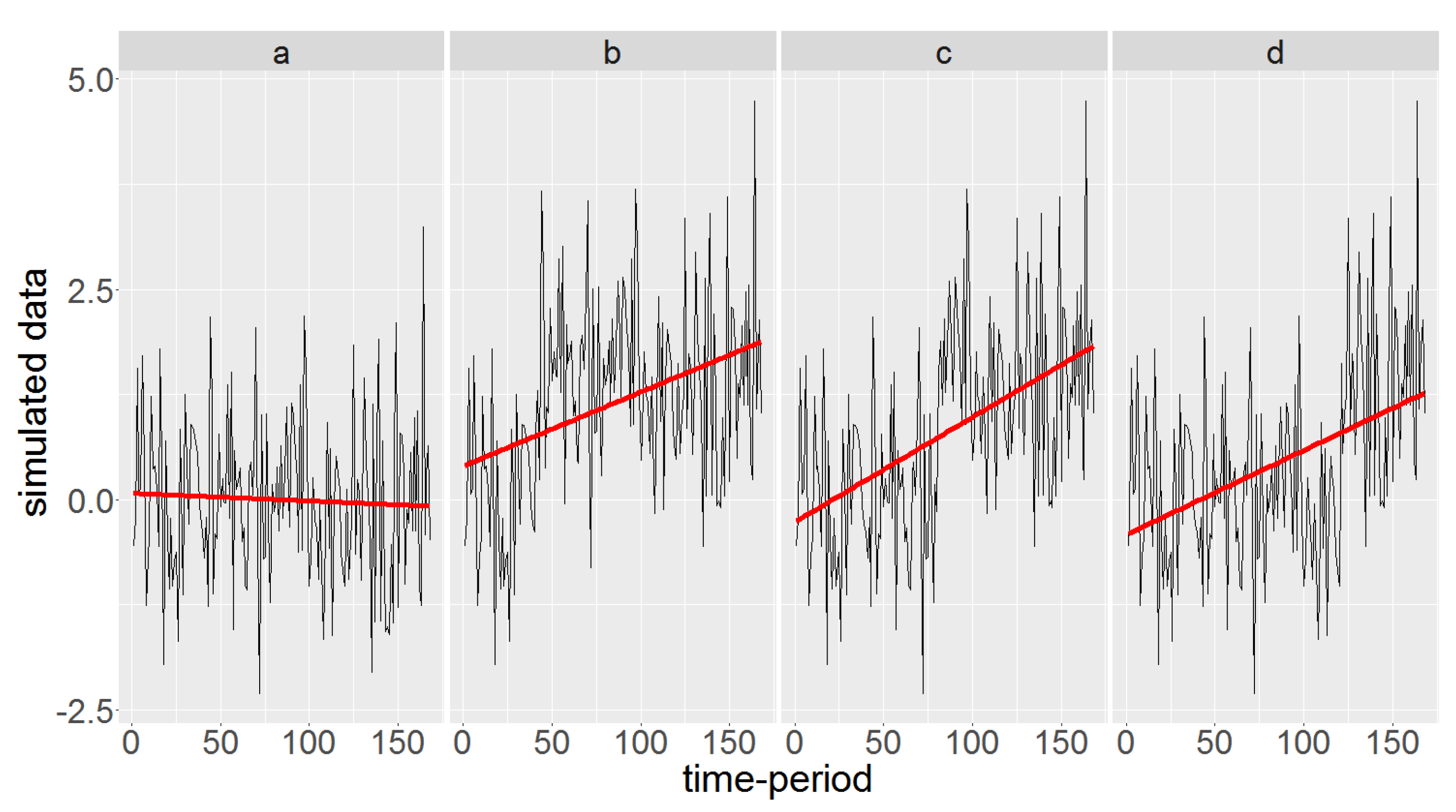
Here we show that an artificial abrupt change in the average might cause a trend. Consider a simulated dataset of length 168 from a standard normal distribution, assumed to be monthly data over 14 years. Figure 3 shows the original data in panel a, and the data with an artificial abrupt change of magnitude 1.5 initiated at the 40th, 80th, and 120th time-periods in panels b, c, and d respectively. The fitted regression line is also displayed in red for each panel, being almost horizontal around the average for the original data with no evidence of trend. The slopes of the fitted regression lines for panels b, c, and d are, however, statistically significant, showing an upward trend. Generally, the closer the change-point to the middle of time period, the steeper the slope of the fitted regression line.
Note that here we produce an artificial abrupt change in a time series that does not contain any trend by definition. This example indeed illustrates a situation in which trend detection methods might actually be able to detect the existence of abrupt changes in time-ordered datasets. See [3] for situations where a change-point can mask a trend or vice versa.
3. Simulation Study
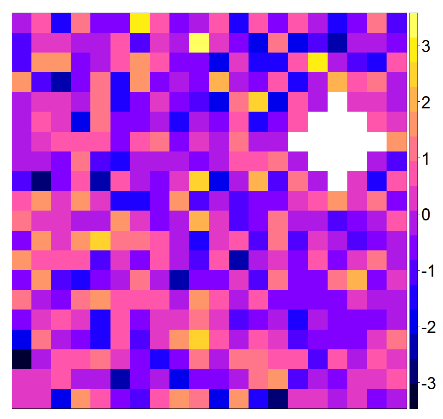
In this section, we describe a simulation study for assessing and comparing the performances of the methods presented in Section 2. We consider two scenarios each based on 100 multi-layer rasters [50] of 168 layers corresponding to 14 years by 12 months. All rasters are within the unit box, and with resolution which yields 400 pixels. In fact, for each scenario we simulate 40,000 time series of length 168. In the first scenario, time series are generated from the standard normal distribution, whereas in the second scenario we simulate time series from an autoregresive model with coefficient 0.8. For both scenarios pixel time series are independent with respect to each other. We produce artificial abrupt changes in a randomly selected cloud containing 13 joint pixels. Figure 4 shows a simulated raster from the first scenario and a randomly selected cloud displayed in white. The pixels falling in this cloud are used as locations in which we produce artificial abrupt changes. Throughout this section, the cloud will be used as an outbreak of abrupt changes established by adding or units to the original simulated data inside the cloud from the starting time-periods onward. For instance, if the magnitude of change 0.5 and time-period 40 are considered, this means that we add 0.5 to data that appeared at any time later than 39.
We considered different benchmarks for comparing the performances of the methods inside and outside the cloud based on 100 simulated multi-layer rasters. We also evaluated their accuracies to check how close the detected change-points were from the true change-points. More precisely, we made use of the following criteria:
- The empirical power of the test is calculated in the cloud where artificial changes are produced, and it is given by dividing the number of detected trend/change-points inside the cloud by the total number of pixels of the cloud. The power of the test is a good indicator with which to reveal how well the methods detect the existence of the produced abrupt change within the cloud.
- The type I error probability is the probability of introducing a false trend/change-point (a false positive). This is estimated by dividing the number of detected change-points outside the cloud by the total number of pixels outside the cloud.
- The mean absolute error (MAE) checks how accurately the methods detect the artificial change-points. This is only calculated for methods that are designed to detect change-points. Assuming a true change-point is placed at time-period k, , the MAE is of the formwhere is the estimated change-point for the j-th pixel of the cloud in the i-th multi-layer raster. Note that 100 is the number of simulated multi-layer rasters, and 13 is the number of pixels falling in the randomly located cloud.
3.1. Computational Details
The use of the trend and change-point detection methods presented in Section 2 was facilitated by several R [51] packages, such as trend [52], modifiedmk [53], changepoint [54], strucchange [25], bfast [27], and ecp [49]. Table 1 highlights the R packages, methods, and functions used in the simulation study. Note that the methods accommodated in modifiedmk [53] are in fact modified versions of the Mann–Kendall method to deal with autocorrelated data [30,31,32,33,34].
The functions mmky1lag and mmkh3lag use the same techniques as mmky and mmkh respectively, but based on their first and the first three autocorrelation coefficients. In addition, when using Meanvar we consider the method AMOC (at most one change since we produce only a single change), the penalty function SIC (Schwarz information criterion), the normal test statistic, and the minimum number of observations between change-points equal to 25. The Strucchange technique is run with minimum number of observations between change-points proportional to of the data size. When using BFAST we consider a minimum number of observations between change-points proportional to of the data size, a maximum number of iterations equal to 1, and no seasonal model, since we do not consider seasonal trend in our simulation process. In the E.divisive method we use the maximum number of random permutations equal to 299, the minimum number of observations between change-points equal to 25, and moment index 1. For those methods that need to set the minimum number of observations between change-points in advance, we use equivalent values. We note that when increasing the minimum number of observations between change-points, the power of the test to detect changes at initial and/or ultimate time-periods is reduced. Consequently, the power to detect all possible significant change-points is also reduced. Therefore, it is recommended to keep this number as small as possible. A significance level is considered in all the performed tests. The R packages sp [55,56] and ggplot2 [57] are used for graphical provisioning.
3.2. Scenario 1: Normally Distributed Remote Sensing Data
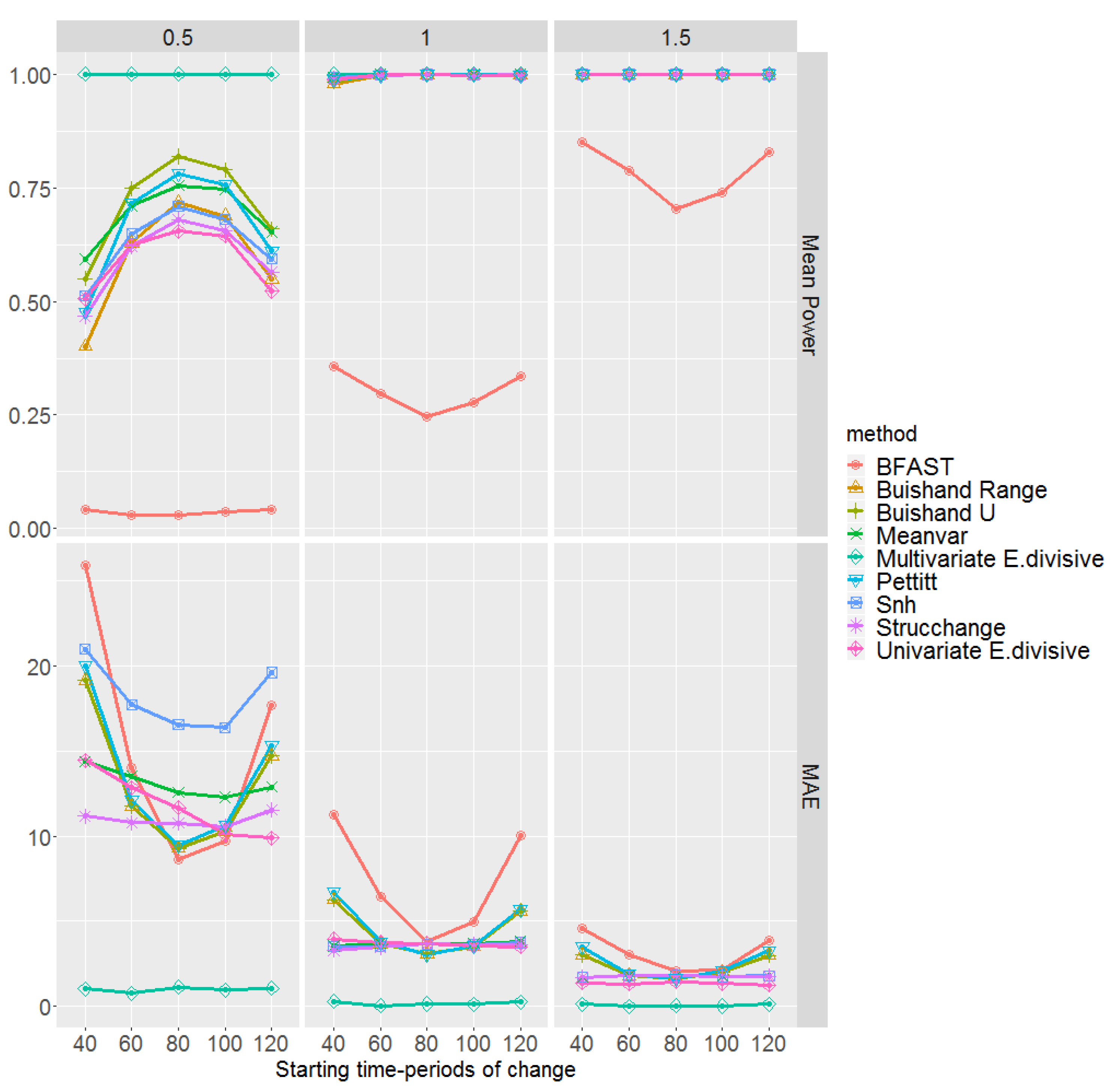
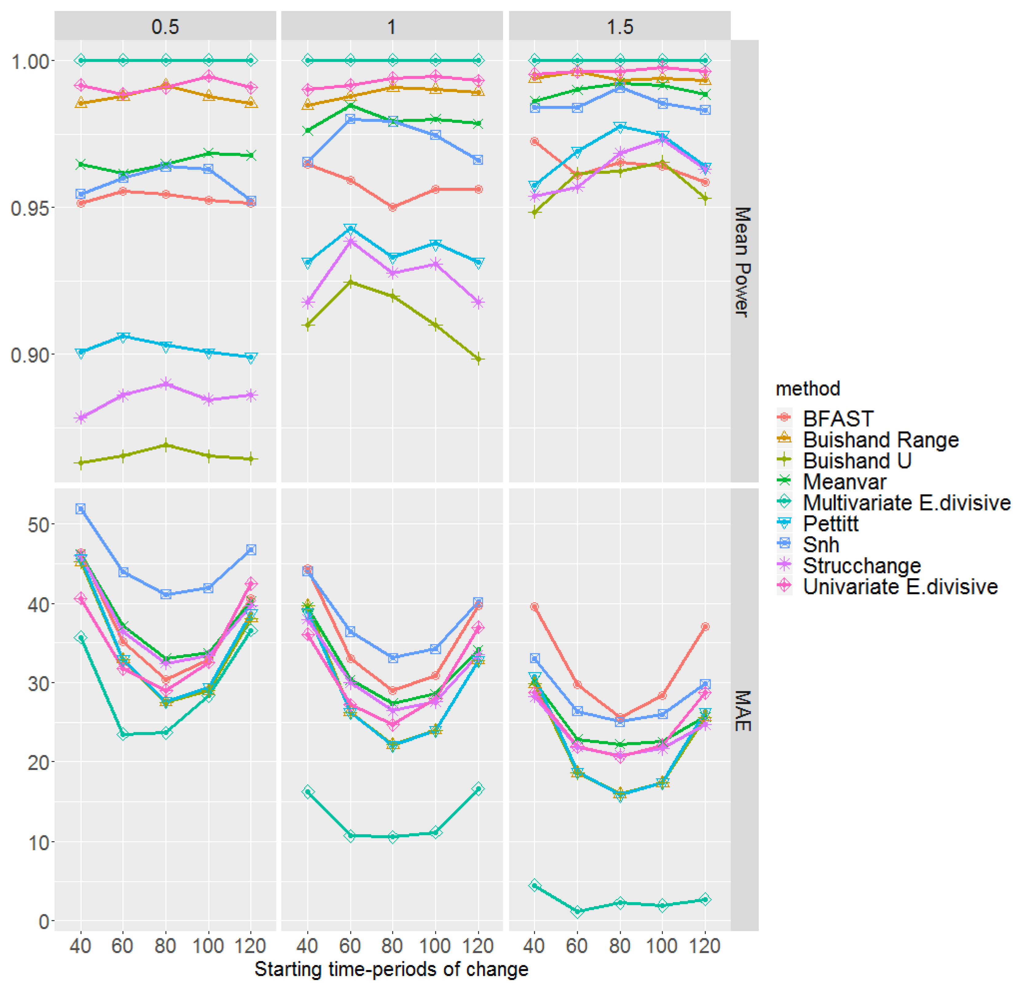
The mean empirical power of the test and MAE, for change-point detection methods, are displayed in Figure 5 with respect to different magnitudes and , and starting time-periods in which their effect on the performance of all methods is visible. These are obtained based on 100 multi-layer rasters. We notice that, regardless of the methods and times of change initialisation, the higher the magnitude of change, the higher the power of the test and the lower the MAE. According to both the power of the test and the MAE, the multivariate E.divisive method uniformly outperforms other methods, having the highest power and the lowest MAE regardless of the magnitude of change. We underline that increasing the size of the cloud might even result in a higher power and lower MAE for the multivariate E.divisive. It is important to note that multivariate methods are not able to identify where dominance occurs. In other words, when applying multivariate methods to multi-layer rasters, they only indicate the time at which a change has happened without pointing out to the location/pixel of the detected change.
Turning to the univariate methods, in particular, for a magnitude of change 0.5, we can see that both the power of the test and the MAE are influenced by the tail of the time series, showing a poorer performance compared to the case in which an abrupt change occurs at a middle time-period. Amongst all, BFAST performs the poorest. We highlight that BFAST makes use of the OLS-MOSUM test in which its power decreases when the minimum number of observations between change-points decreases (see Section 2.2.6). Therefore, the performance of BFAST to detect changes in middle time-periods might be improved by increasing this argument; however, it then fails to detect changes in the tails. Equivalent values for such arguments are considered for different methods if needed. We also observe in Figure 5 that, for magnitudes of change 1 and 1.5, the MAEs of the Strucchange, univariate E.divisive, Meanvar, and Snh methods are less affected in the tails than the case for the BFAST, Buishand Range, Buishand U, and Pettitt methods. Apparently, amongst univariate change-point detection methods and based on magnitudes of change 1 and 1.5, the methods Strucchange, E.divisive, Snh, and Meanvar are overall the preferable choices. We highlight that for magnitudes larger than 1.5, all methods perform quite well.
We mention the fact that, in practice, the methods univariate E.divisive, Strucchange, Meanvar, and BFAST sometimes did not detect any change, and as a result, it was not possible to compute the MAE. Then, the MAE results displayed in Figure 5 were obtained based on change-points detected. The implementation of the methods Buishand Range, Buishand U, Snh, and Pettitt in the R package trend [52] identifies the most probable change-point, even if it is not significant. This probable change-point was used for MAE calculation regardless of it being significant or not.
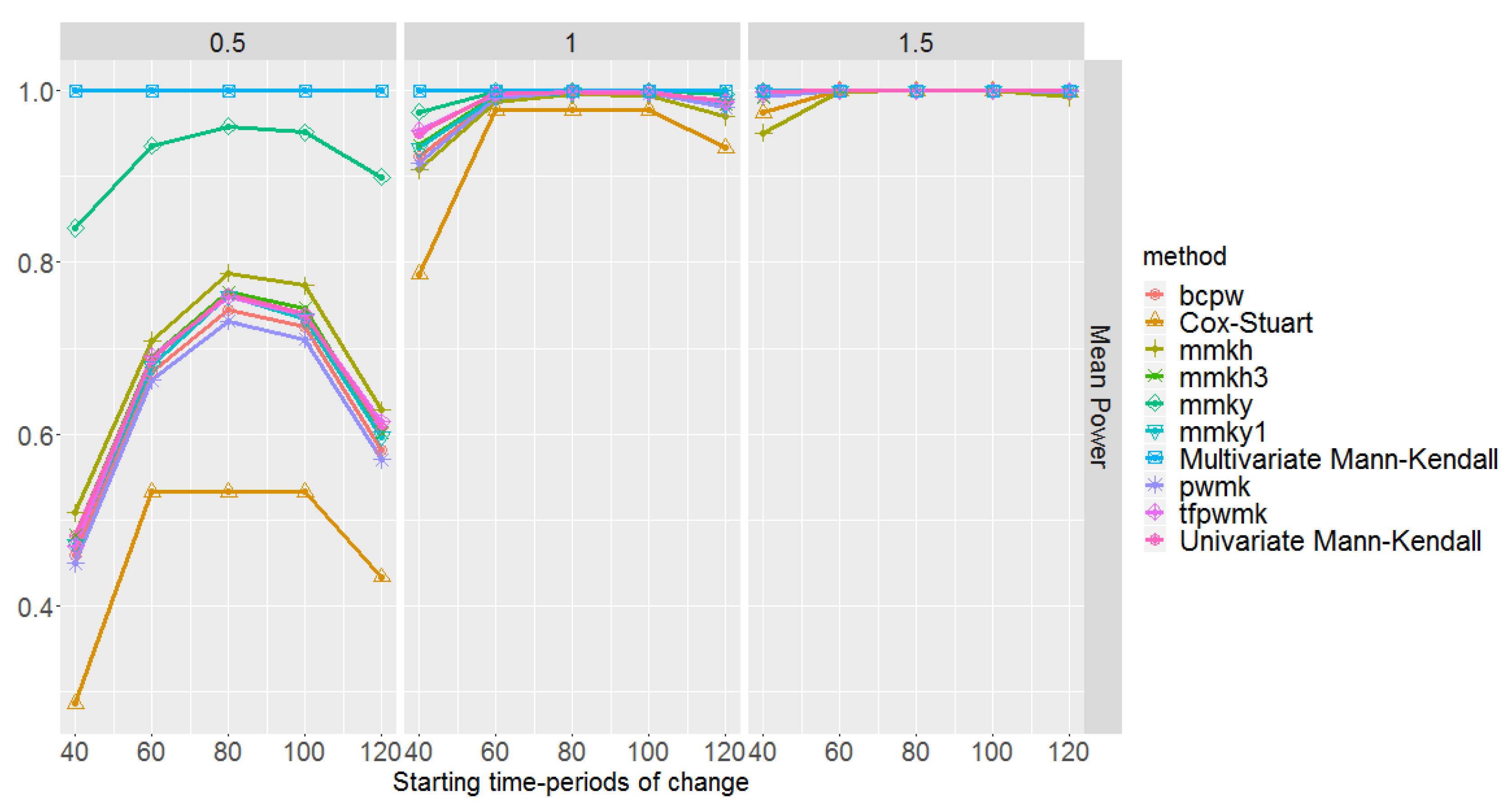
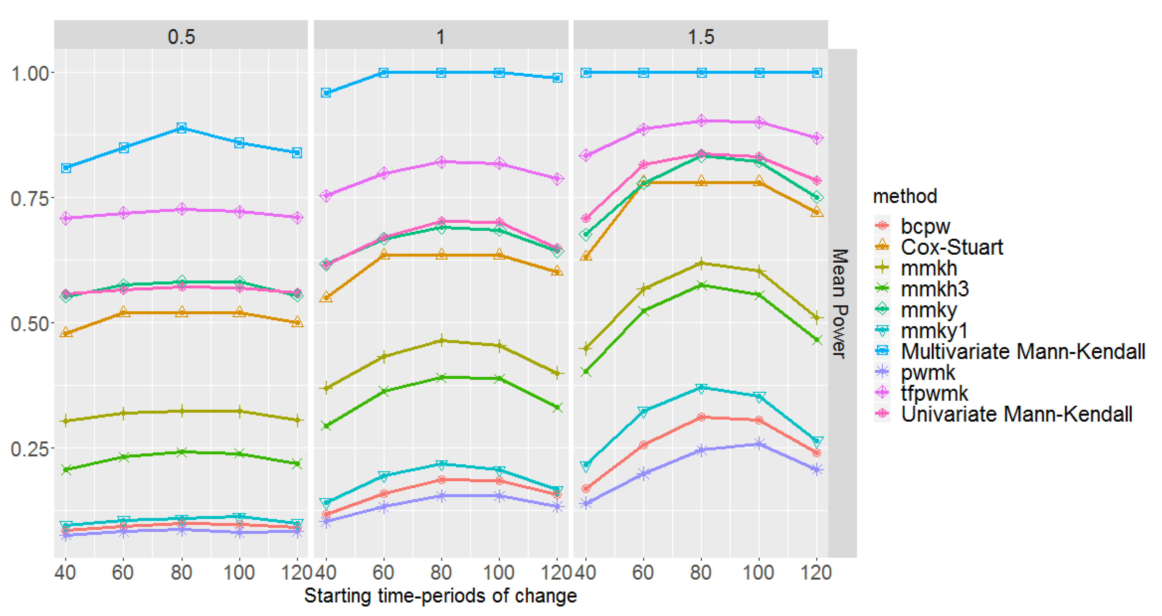
Figure 6 shows the mean empirical power of the test for each of the trend detection methods. Amongst all methods, multivariate Mann–Kendall performs the best irrespective of the magnitude of change and starting time-period. All the univariate methods, however, suffer from detecting a trend when an abrupt change is placed in a tail, especially for small magnitudes of change. Nevertheless, the Yue and Wang variance-corrected univariate Mann–Kendall approach (mmky) [33] outperforms others showing a fairly high power. The Cox–Stuart method has the lowest power. The methods mmkh, mmkh3, mmky1, pwmk, and tfpwmk exhibit similar performances, showing a higher power than Cox–Stuart but lower power than mmky. For all the univariate methods and for small magnitudes of change, the power curve is symmetric with a peak at a middle time-period.
The power of the test and the MAE are not enough to assess the performance of the methods. Table 2 shows the mean type I error probability of the methods based on 100 multi-layer rasters. Excluding mmky and BFAST, since they have the highest () and lowest () type I error probabilities respectively, the rest of the methods show similar performances having average type I error probabilities between and . Taking a closer look to the behaviour of the univariate methods in Figure 5 and Figure 6, and Table 2, we realise that mmky which has the highest power, suffers the most from false positives, and BFAST, which has the lowest type I error probability, is incapable of detecting actual changes properly. This indeed highlights the close relation between the type I error probability and the power of the test.
In summary, combining the results of Figure 5 and Figure 6 with Table 2, we conclude that multivariate E.divisive and Mann–Kendall outperform the univariate methods, yet are incapable of pointing out where dominance occurs. Regarding univariate methods, after excluding mmky and BFAST due to their having a high type I error probability and low power respectively, the other methods perform similarly.
3.3. Scenario 2: Autoregressive Remote Sensing Data
In this scenario we simulate 100 multi-layer rasters with pixel time series generated from an autoregressive model with parameter . Hence, the variation is higher and there are more jumps compared to Scenario 1. Figure 7 shows the mean empirical power of the tests together with the MAE of change-point detection methods. Similarly to Scenario 1, the multivariate E.divisive method outperforms other methods based on both power and MAE. However, its MAE is greater than that of Scenario 1. This seems reasonable, as this method assumes independence.
With respect to the behaviour of univariate methods in mean power, they show less sensitivity in the tails, and less power for magnitudes 1 and 1.5 than in Scenario 1. Both the univariate E.divisive and Buishand Range methods have the highest power irrespective of the time-period. Generally, the MAEs of all methods in Scenario 2 are higher than in Scenario 1, which might be a sign of having higher type I error. Similarly to Scenario 1, for all methods, MAE is smaller for middle time-periods. Apparently, Buishand U, Buishand Range, and Pettitt methods show the lowest MAEs, whereas the highest MAE is shown jointly by the Snh and BFAST methods. In summary, Buishand Range is the preferable method, since it has the highest power and the lowest MAE among univariate methods. We emphasise that for magnitudes larger than 1.5, all methods perform quite well. As in Scenario 1, Meanvar, BFAST, Strucchange, and univariate E.divisive do not necessarily detect a change.
Figure 8 shows the mean empirical power of the tests for the methods originally designed for trend detection. Regardless of the magnitude of change and time-period, the multivariate Mann–Kendall outperforms other methods, showing a fairly high power. Concerning the univariate methods, the highest power is attained by tfpwmk, the trend-free pre-whitened version of Mann–Kendall proposed by Yue et al. [32], and the second highest power belongs to univariate Mann–Kendall and mmky, the variance-corrected version of Mann–Kendall proposed by Yue and Wang [33].
To get a better insight into the performances of the different methods, their mean probability of committing a type I error is given in Table 3. Apart from the methods pwmk, mmky1, and bcpw that have very low type I error, there is a clear reduction in the performance of other methods showing high probabilities of committing a type I error. Yet the trend detection methods are the least affected ones. Note that pwmk, mmky1, and bcpw are the methods with the lowest power. This being said, a preferable method should be selected based on maximising the power of the test and minimising the type I error probability jointly. Hence, looking for a balance between the power of the test and type I error probability leads us to the original Mann–Kendall.
3.4. Summary
Trend detection methods can also be used to detect the existence of abrupt changes, since they might provoke a monotonic trend, as has been shown in Section 2.3. However, it is then not obvious to distinguish an inherent trend from a trend caused by an abrupt change. In addition, in case a trend is caused by an abrupt change, trend detection methods are not able to point out the time-period of such change.
The results obtained in Scenarios 1 and 2 underline the poor performance of trend and change-point detection methods in the presence of autocorrelation. The stronger the degree of autocorrelation, the higher the type I error probability [30,31,32,33,34,35]. It is of great importance to remember the relationship between the power of the test and the type I error probability. Reducing the probability of committing a type I error might actually result in an undeniable decrease of the power of the test, as is seen in the performance of the different corrections applied to the Mann–Kendall test when dealing with autocorrelated data. Thus, aiming at finding a trade-off between maximising the power of the test and minimising the type I error probability jointly, the original Mann–Kendall is generally the preferable method. Although it cannot reveal the time-period that an abrupt change occurs, its result regarding the presence of a change-point is more reliable than other methods. Nevertheless, if we were to choose a change-point method when there is a weak autocorrelation in the data, our choice is Strucchange, since it slightly outperforms other change-point methods based on a balance between the power of the test, type I error probability, and MAE.
4. Remote Sensing LST Data of Navarre, Spain
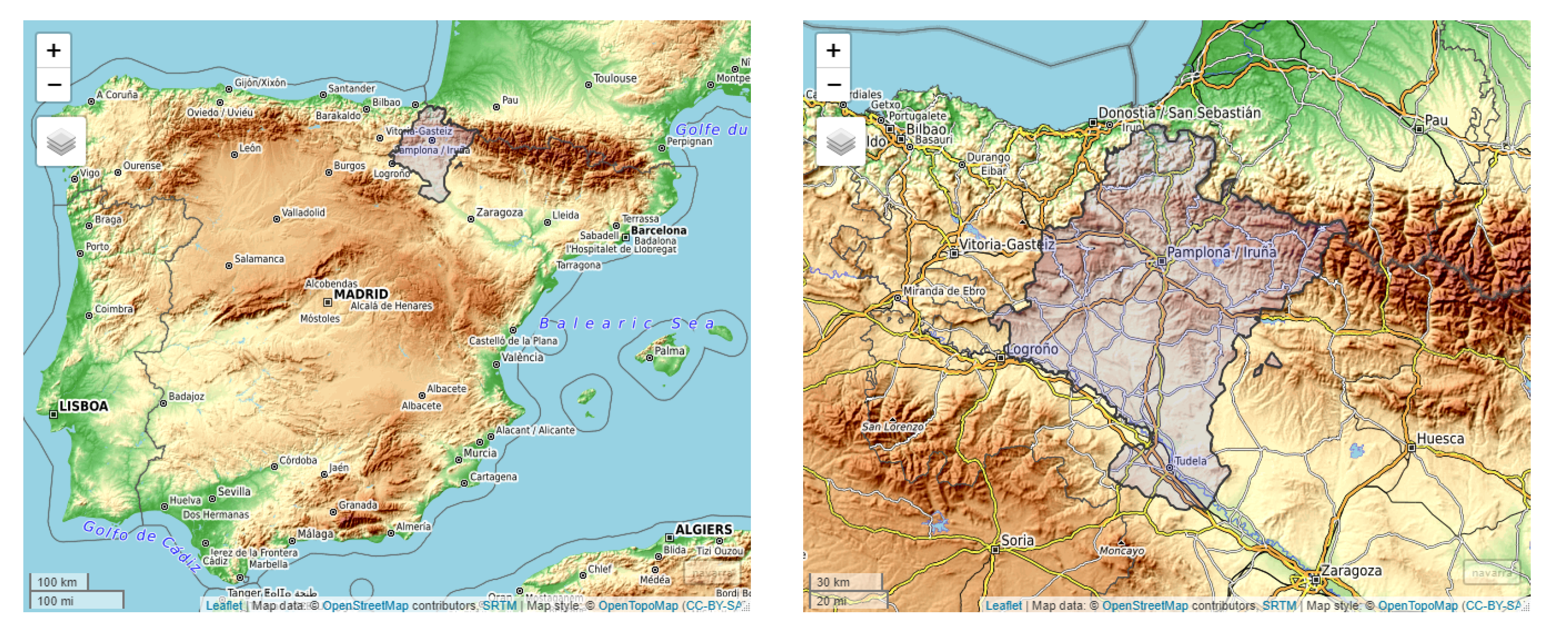
Figure 9 shows the map of Navarre, obtained through the R package mapview [58]; it is a region located in the north of Spain with an area of approximately 10,000 km. The climate varies across the province of Navarre. The north-west is influenced by Atlantic Ocean and it has a humid coastal-type climate. It is made up of several valleys. The north-east of Navarre has a higher altitude, lower average temperature, and higher rainfall than other zones in the region. Precipitation is high in the north and tapers off toward the south, which is mostly formed by lowland area with dry summers, large annual variations in temperature, and little and irregular rainfall.
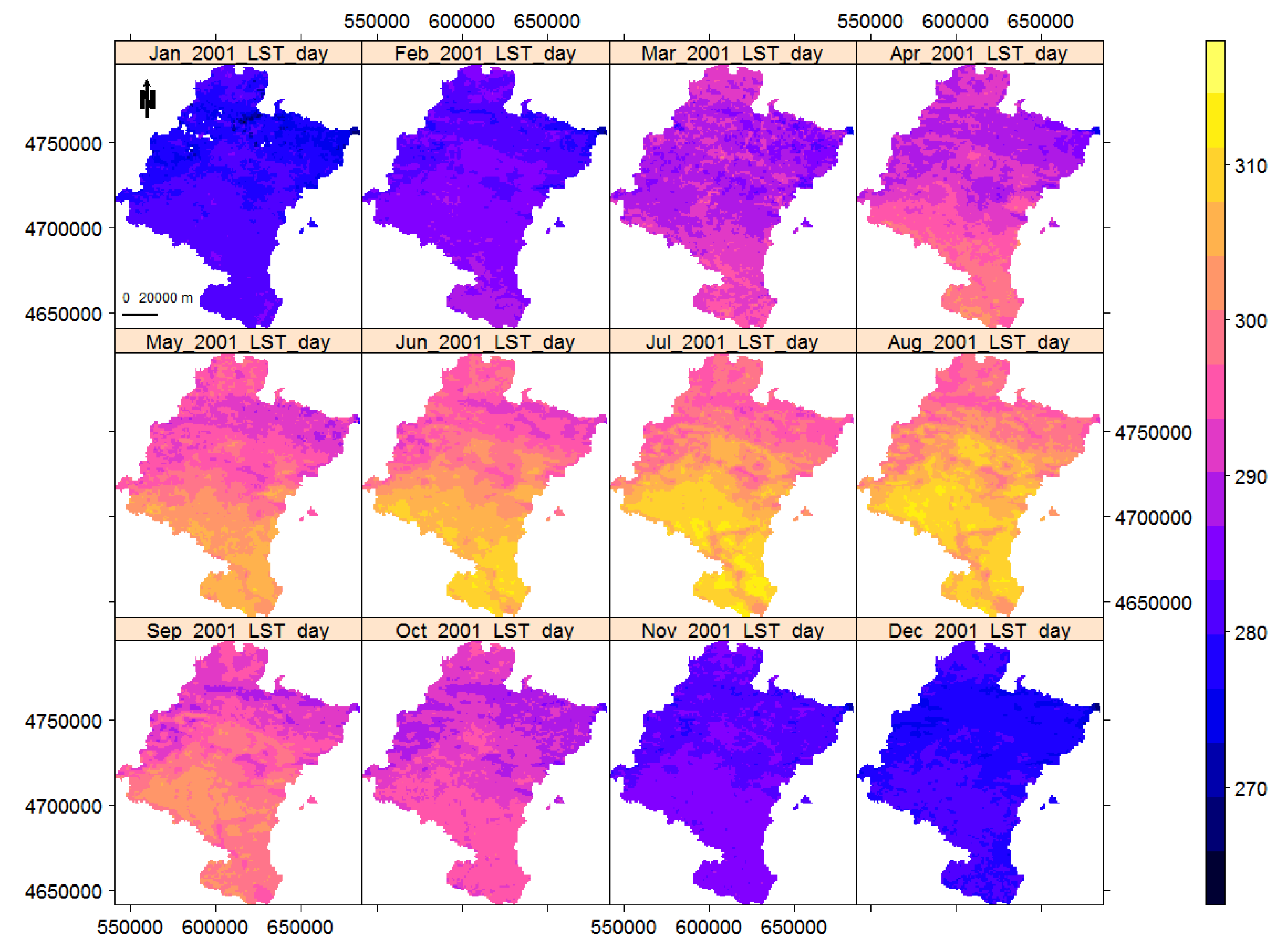
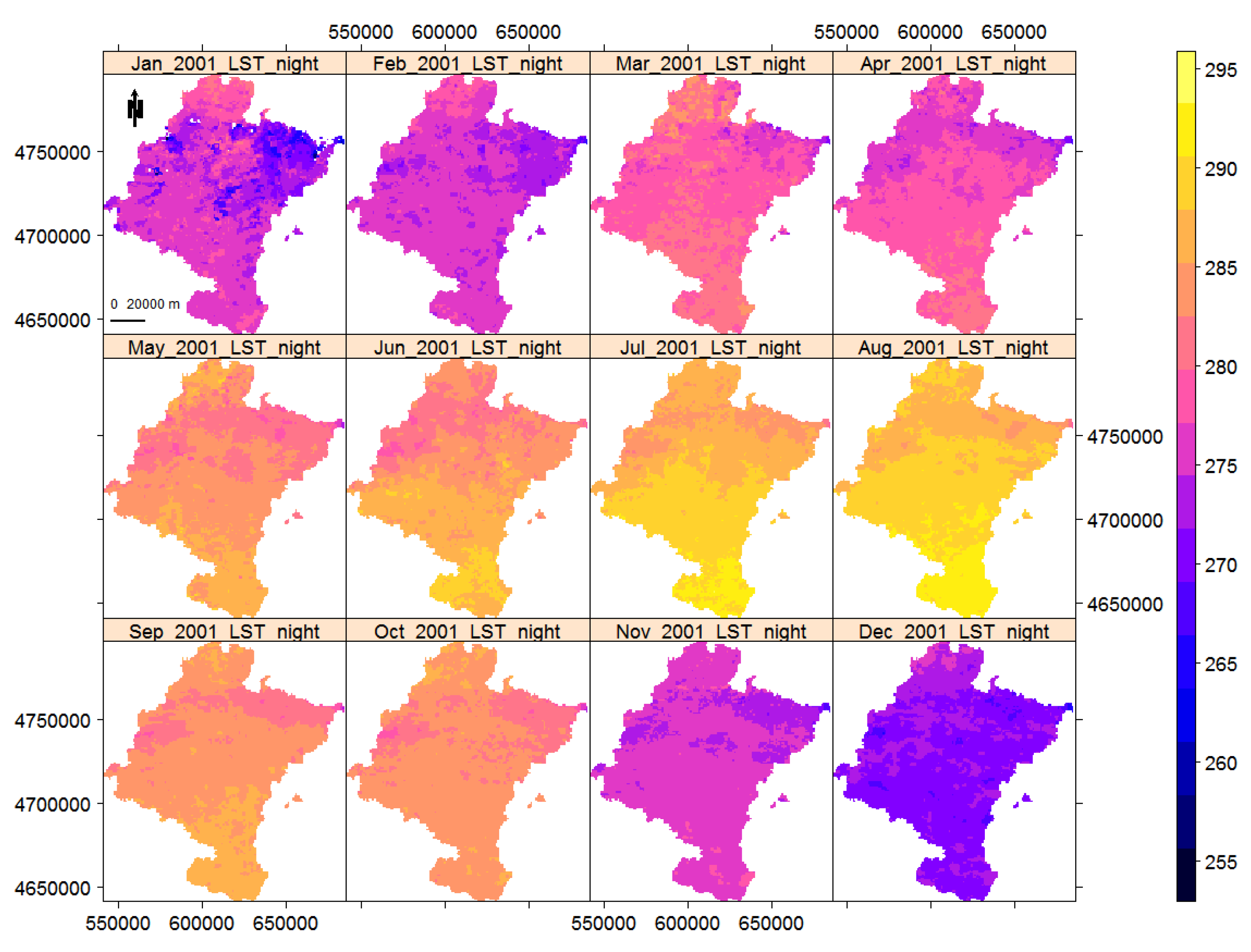
The availability of remote sensing LST data through different satellites provides the opportunity to monitor their changes over time. In this section, we illustrate the detection of trend/change-points with two real time-series of LST day and night satellite images of Navarre, from January 2001 to December 2018. The original images are eight-day composite images from version-6 MOD11A2, product of MODIS. The images were acquired through Terra satellite at 10:30 and 22:30 local time. This product was derived from the two thermal infrared (TIR) channels: 31 (10.78 to 11.28 μm) and 32 (11.77 to 12.27 μm) [59], wherein the split-window algorithm [60] is used for correcting the atmospheric effects. Images have been downloaded, customised, and monthly-averaged using the R package RGISTools [51,61]. The images are UTM projected; they are loaded into R as multi-layer rasters; and their LST values are in Kelvin degrees. The original MOD11A2 images are factor scaled by 0.02, meaning that we obtain the Kelvin degrees when multiplying by this factor. Each LST time series of images has 216 layers, a byproduct of 18 years by 12 months. The spatial resolution of each tile is , including 25,410 pixels of approximately 1 km from which 11,691 pixels are enclosed inside Navarre borders. Figure 10 and Figure 11 show the LST day and night monthly images of Navarre in 2001 as showcases. Generally, the changes of LST over months are visible, with lower temperature for LST night and higher variation for LST day. Furthermore, Table 4 shows the descriptive statistics of remote sensing LST data over different seasons. In addition—and regardless of month—day and night, the lowest LST belongs to the north-east of Navarre, which is a mountainous region.
Results
We now employ both the multivariate and univariate Mann–Kendall [13,14,52,62] to look for locations with significant trend in the time-series of LST day and night images of Navarre. We here only focus on the deseasoned data. Therefore, we first deseason the data using the deseason function of the R package remote [63] that creates seasonal anomalies of data. In other words, each deseasoned image is obtained by subtracting the average image of its corresponding month over all the time period from the target image. We further consider averaging data in windows with the aggregate function from the R package raster [50]. Although this aggregation may be done with other aggregation factors or even avoided, it smooths data and might reduce potential false positives. Hereafter, we use the deseasoned and aggregated LST remote sensing data.
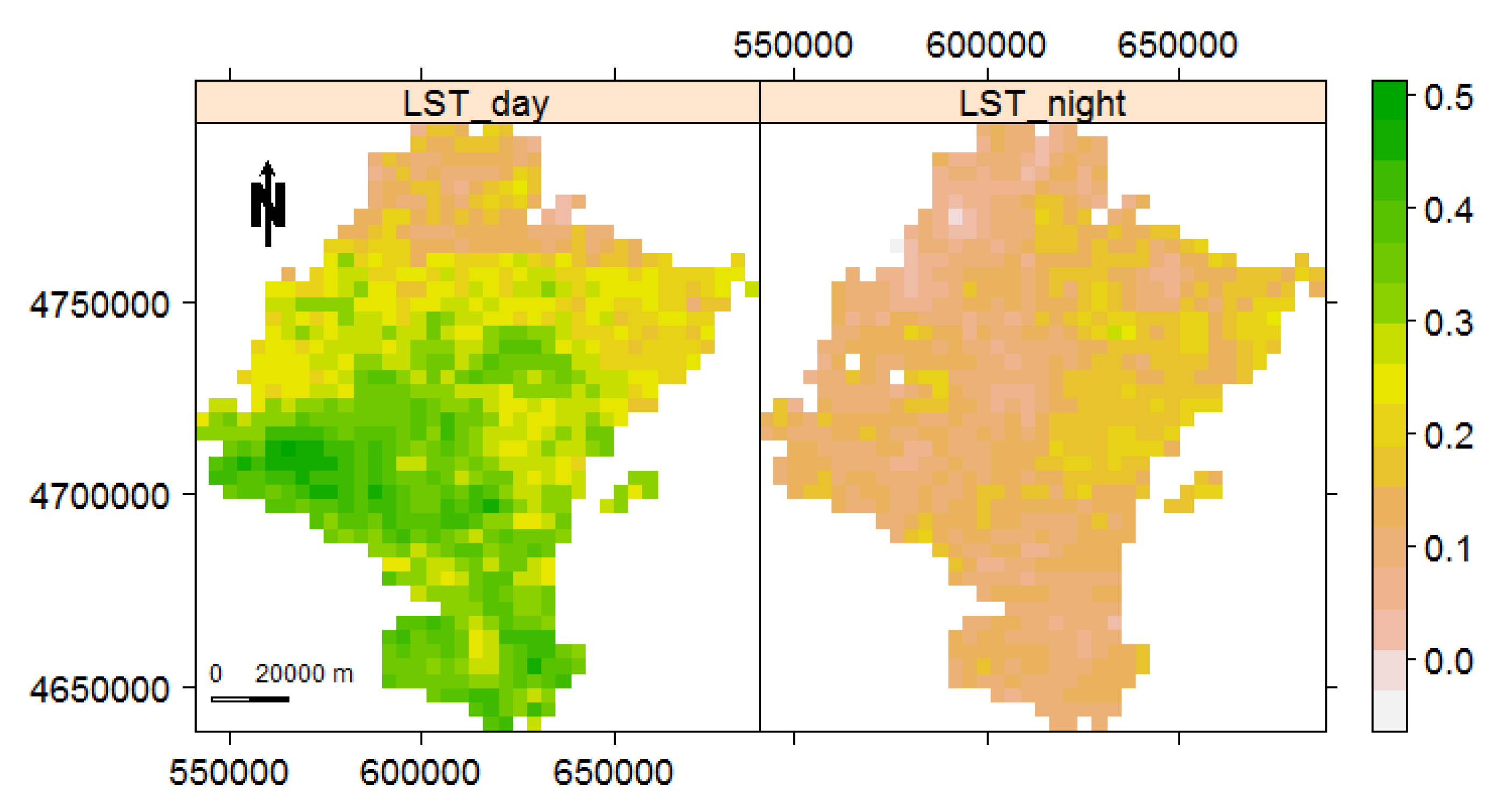
Being aware of the effect of autocorrelation on the performance of Mann–Kendall, we next check the presence of temporal autocorrelation for both LST day and night by calculating the first lag of the partial autocorrelation function over each pixel time series. Figure 12 shows how the first lag partial autocorrelation for monthly remote sensing LST data of Navarre, Spain, varies across the region. For LST day, the temporal autocorrelation is increasing from the north towards the south of Navarre. The LST night, however, shows its highest degree of temporal autocorrelation in the north-east of Navarre. This variation might be due to the variety of land cover, vegetation, altitude, moisture, precipitation, and so forth. Generally, taking Figure 10 and Figure 11 into account, for LST day the regions with low temperatures (north) have weaker autocorrelation, while for LST night the regions with lower temperatures (north-east) have stronger autocorrelation.
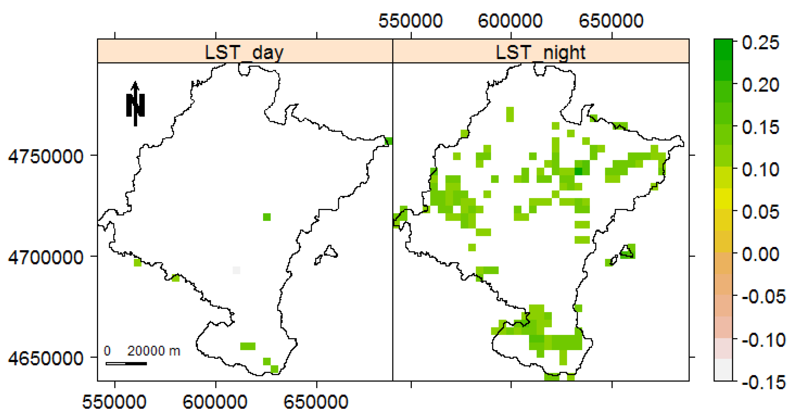
The multivariate Mann–Kendall does not detect any trend for LST day (p-value = ), but identifies a monotonic trend for LST night (p-value = ). Since multivariate methods do not point out where dominance occurs, we next use the univariate Mann–Kendall to check the existence of trend in each pixel individually. Figure 13 shows the detected pixels with significant trends at a significance level to require stronger evidence, for LST day and night images of Navarre from January 2001 to December 2018. The number of detected pixels for LST night is higher than LST day. Taking the map of Navarre, displayed in Figure 9, into account, we underline that the detected locations in the south of Navarre belong to a zone with both agricultural and urban land-cover. This area is also exposed to warmer weather than the north (see Figure 10 and Figure 11). The Ebro river, that is, the most important river in Spain in terms of length and area of drainage basin, also flows through this area. Although a few pixels detected in the north-west and north-east of Navarre are located in urban regions, most of the pixels detected belong to green areas and mountainous regions. Note the high power and low type I error probability of Mann–Kendall in the presence of weak autocorrelation.
In Section 3 we have already seen that one disadvantage of trend/change-point detection methods in general is the rate of false positives, especially in the presence of temporal autocorrelation. Being aware of our finding in Figure 12, we cannot certainly conclude whether those pixels detected in Figure 13, in particular for LST day, are correctly detected or not. In addition, we are not able to identify the trend caused by an abrupt change. We accentuate that distinguishing real change-points from false positives when analysing real datasets needs further research.
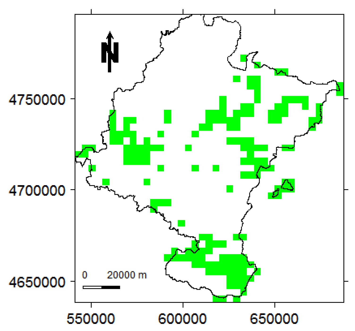
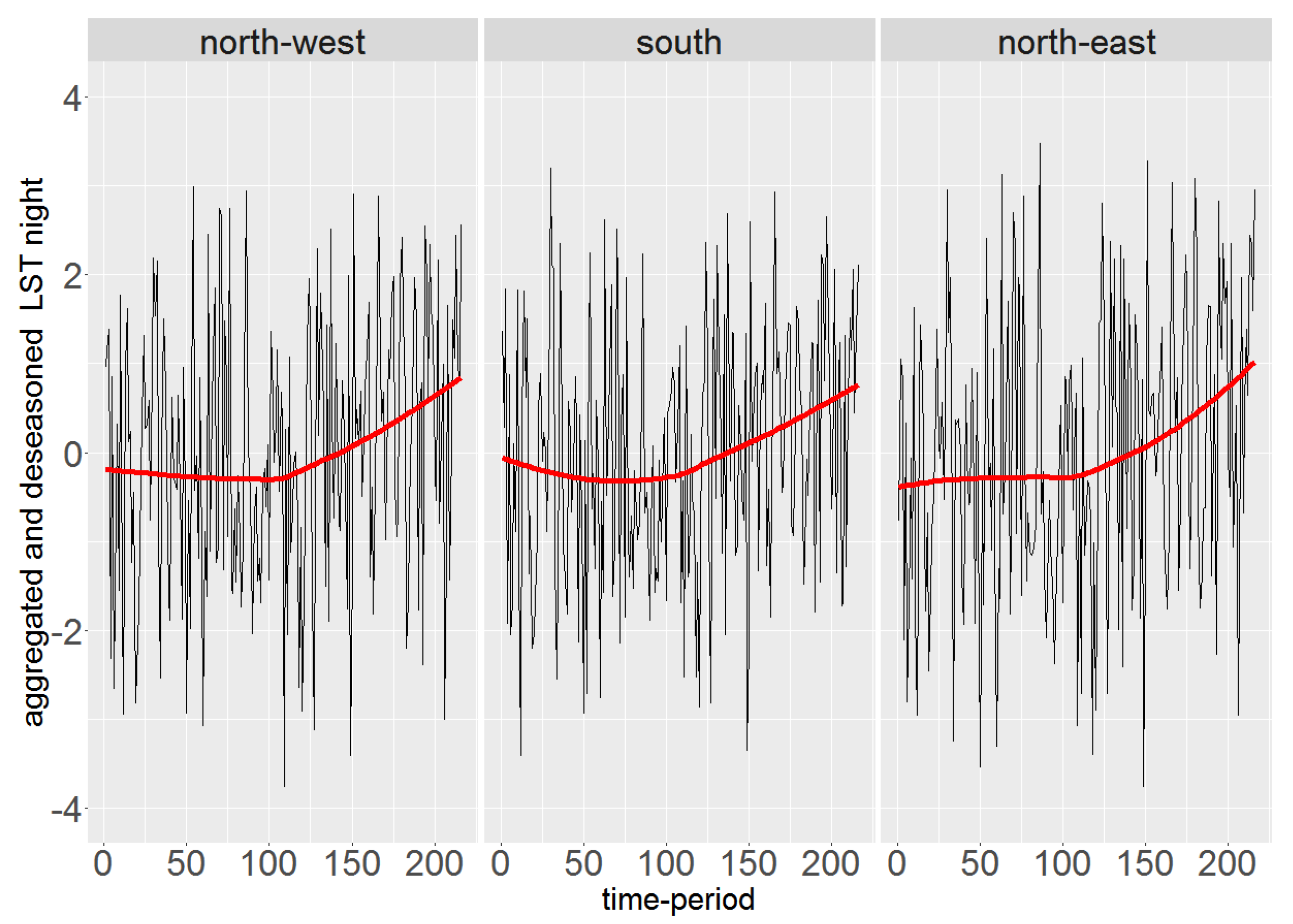
Since LST night images show a low degree of autocorrelation ranging from –0.03 to 0.28, as an extra step, we employ the Strucchange method to check for the existence of change-points in the LST night data. Note that, for data with low degree of autocorrelation, Strucchange slightly outperforms other change-point detection methods in terms of a trade-off between power of the test, type I error probability, and MAE. Figure 14 shows the detected locations facing change-points based on Strucchange. The majority of these changes were detected in January 2011 and June 2013. It is worth noting that of the locations detected by Strucchange were also detected by Mann–Kendall. The pixels detected by both Mann–Kendall and Strucchange methods are basically placed in three areas located in the north-east, north-west, and south of Navarre respectively. In each of these areas the behaviour of the pixel time series is similar; thus we look into their average behaviour. Figure 15 shows the averages of the corresponding pixel time series from each area in combination with their locally weighted smooth regression lines in red [64]. We can see that LST night in all three areas shows consistent behaviour, being flat until the middle of the time series and then having an upward trend. This in fact shows a situation that both trend and change-points exist in the time series.
5. Conclusions and Discussion
Aside from reviewing several trend and change-point detection methods, this paper has shown a simulation study used to assess and compare the performances of different methods, such as (modified) Mann–Kendall, Cox–Stuart, Pettitt, Buishand range, Buishand U, Snh, Meanvar, Strucchange, BFAST, and E.divisive in terms of their detecting abrupt changes for time-ordered multi-layer rasters. We have considered two scenarios according to which pixel time series are simulated from the standard normal distribution in the first scenario, whereas an autoregressive model with parameter 0.8 was considered for the second scenario. In each scenario, 100 multi-layer rasters, of dimensions pixels, with 168 layers, were simulated, providing a total of 40,000 time series of 168 pixels. We created a randomly selected cloud consisting of 13 joint pixels in which we produced artificial abrupt changes. The magnitudes of change and the starting time-periods were considered. Then, the pixel time series inside the cloud were modified by summing 0.5, 1 or 1.5 units to the their original values from a starting time-period onward. We have not made any changes outside the cloud. Since the artificial change-points are located in the cloud, we focused on the mean empirical power of the test, together with MAE in the cloud, and the mean probability of introducing false positives outside the cloud, as performance criteria. For all methods we considered a significance level.
The simulation study demonstrated that the performances of all methods are strongly affected by the existence of temporal autocorrelation. The higher the degree of temporal autocorrelation, the higher the probability of committing a type I error. This drawback was previously seen for Mann–Kendall and Pettitt test [30,31,32,33,34,35]. However, amongst all, the trend detection methods are the least affected ones by temporal autocorrelation. Moreover, for change-point detection methods, the MAE for autocorrelated data is greater than that of independent data. In addition, all methods have faced difficulties to detect changes at the first and last time-periods. This is not clearly visible for data with strong temporal autocorrelation due to the high type I error probability in this case. The proposed corrections to the Mann–Kendall method [30,31,32,33,34], for autocorrelated data, aiming at reducing or moderating its type I error probability, clearly affect its power. In other words, although these corrections might reduce the type I error probability of Mann–Kendall test, they also undeniably decrease its power. Apparently, for such techniques, the relationship between the power of the test and the type I error probability has not received much attention. Nevertheless, considering both the power of the test and the probability of introducing false positives, the original Mann–Kendall method is still the preferable choice. Although Mann–Kendall is not able to identify the time-periods of abrupt changes, it is generally more reliable than other methods when detecting the existence of such changes. Turning to the performance of change-point detection methods for independent data, Strucchange slightly outperforms other methods after making a trade-off between the power of the test, type I error probability, and MAE. In particular, the MAE of Strucchange is more stable than other methods with respect to the starting time-periods of change. Hence, we have also used Strucchange to look for potential change-points in the LST night data of Navarre, as it shows a weak temporal autocorrelation.
With regard to BFAST, Strucchange, Meanvar, and E.divisive methods, which demand identifying the minimum number of data points between any two consecutive change-points in advance, we underline that considering a large value for such argument forces the methods to only detect possible change-points at middle time-periods, and it further reduces the power of the test to detect all potential change-points. Amongst all, BFAST has been the most sensitive method to the choices of such arguments. Since usually there is no previous knowledge about the numbers and positions of change-points, it is recommended to select the number of observations between change-points to be as small as possible. In a case in which we are aware of the existence of a change in a particular period of time without knowing the exact change-point, the pre-selected minimum number of observations between change-points may be chosen accordingly.
Concerning the difference between univariate and multivariate methods, we note that the advantage of the majority of the univariate methods is that both the location and time-period of change can be detected, but the detection process does not take into account any information about the relationship between neighbouring pixels, since each pixel time series is analysed separately. The multivariate methods, however, take the information from all pixel time series at once without pointing to the location of possible change-points. We have excluded the methods E-Agglo [17] and pruned objective [65] from the R package ecp [49], since by default they always introduce at least one change-point.
Regarding future works, since trend detection methods generally show a lower type I error probability than the methods inherently designed for change-point detection, it would be relevant and interesting to modify them adding the possibility of finding the times at which the changes occur. Another relevant idea might be to execute a simulation study based on another type of abrupt change, such as a sudden change in the trend direction.
Author Contributions
A.F.M. proposed and organised the research; M.D.U. contributed to the design of research; and M.M. ran the statistical programs. The three authors all contributed to writing the manuscript. All authors have read and agreed to the published version of the manuscript.
Funding
This work has been supported by Project MTM2017-82553-R (AEI/FEDER, UE). It has also received funding from la Caixa Foundation (ID1000010434), Caja Navarra Foundation, and UNED Pamplona, under agreement LCF/PR/PR15/51100007.
Acknowledgments
The authors are grateful to the editor and three referees for constructive comments. We also thank Manuel Montesino and Unai Pérez-Goya for fruitful discussions.
Conflicts of Interest
The authors declare no conflict of interest.
Abbreviations
The following abbreviations are used in this manuscript:
| bcpw | Mann-Kendall bias corrected pre-whitening approach of Hamed [34]. |
| BFAST | breaks for additive season and trend. |
| E.divisive | hierarchical divisive. |
| MAE | mean absolute error. |
| Meanvar | Identifying changes using both mean and variance. |
| mmkh | Mann–Kendall variance corrected approach of Hamed and Rao [30]. |
| mmkh3 | Mann–Kendall variance corrected approach of Hamed and Rao [30] by considering only the first three lags. |
| mmky | Mann–Kendall variance corrected approach of Yue and Wang [33]. |
| mmky1 | Mann–Kendall variance corrected approach of Yue and Wang [33] by considering only the first lag. |
| MODIS | Moderate Resolution Imaging Spectroradiometer. |
| LST | land surface temperature. |
| pwmk | Mann–Kendall pre-whitening approach of Von Storch [31]. |
| Snh | standard normal homogeneity. |
| Strucchange | structure change. |
| TIR | thermal infrared. |
| tfpwmk | Mann–Kendall trend-free pre-whitening approach of Yue et al. [32]. |
| UTM | universal transverse mercator. |
References
- Montanez, G.D.; Amizadeh, S.; Laptev, N. Inertial hidden markov models: Modeling change in multivariate time series. In Proceedings of the Twenty-Ninth AAAI Conference on Artificial Intelligence, Austin, TX, USA, 25–30 January 2015. [Google Scholar]
- Aminikhanghahi, S.; Cook, D.J. A survey of methods for time series change point detection. Knowl. Inf. Syst. 2017, 51, 339–367. [Google Scholar] [CrossRef] [Green Version]
- Sharma, S.; Swayne, D.A.; Obimbo, C. Trend analysis and change point techniques: A survey. Energy Ecol. Environ. 2016, 1, 123–130. [Google Scholar] [CrossRef] [Green Version]
- Vicente-Serrano, S.M.; Cabello, D.; Tomás-Burguera, M.; Martín-Hernández, N.; Beguería, S.; Azorin-Molina, C.; Kenawy, A.E. Drought variability and land degradation in semiarid regions: Assessment using remote sensing data and drought indices (1982–2011). Remote Sens. 2015, 7, 4391–4423. [Google Scholar] [CrossRef] [Green Version]
- Xu, X.; Huang, X.; Zhang, Y.; Yu, D. Long-term changes in water clarity in Lake Liangzi determined by remote sensing. Remote Sens. 2018, 10, 1441. [Google Scholar] [CrossRef] [Green Version]
- Wang, Y.; Huang, X.; Liang, H.; Sun, Y.; Feng, Q.; Liang, T. Tracking snow variations in the Northern Hemisphere using multi-source remote sensing data (2000–2015). Remote Sens. 2018, 10, 136. [Google Scholar] [CrossRef] [Green Version]
- Li, Q.; Lu, L.; Weng, Q.; Xie, Y.; Guo, H. Monitoring urban dynamics in the southeast USA using time-series DMSP/OLS nightlight imagery. Remote Sens. 2016, 8, 578. [Google Scholar] [CrossRef] [Green Version]
- NourEldeen, N.; Mao, K.; Yuan, Z.; Shen, X.; Xu, T.; Qin, Z. Analysis of the spatiotemporal change in Land Surface Temperature for a long-term sequence in Africa (2003–2017). Remote Sens. 2020, 12, 488. [Google Scholar] [CrossRef] [Green Version]
- Luo, Z.; Yu, S. Spatiotemporal variability of land surface phenology in China from 2001–2014. Remote Sens. 2017, 9, 65. [Google Scholar] [CrossRef] [Green Version]
- Yang, L.; Jia, K.; Liang, S.; Liu, M.; Wei, X.; Yao, Y.; Zhang, X.; Liu, D. Spatio-temporal analysis and uncertainty of fractional vegetation cover change over northern China during 2001–2012 based on multiple vegetation data sets. Remote Sens. 2018, 10, 549. [Google Scholar] [CrossRef] [Green Version]
- Song, Y.; Jin, L.; Wang, H. Vegetation changes along the Qinghai-Tibet Plateau engineering corridor since 2000 induced by climate change and human activities. Remote Sens. 2018, 10, 95. [Google Scholar] [CrossRef] [Green Version]
- Li, J. Pollution trends in China from 2000 to 2017: A multi-sensor view from space. Remote Sens. 2020, 12, 208. [Google Scholar] [CrossRef] [Green Version]
- Mann, H.B. Nonparametric tests against trend. Econom. J. Econom. Soc. 1945, 13, 245–259. [Google Scholar] [CrossRef]
- Kendall, M.G. Rank Correlation Methods; Griffin: Oxford, UK, 1948. [Google Scholar]
- Cox, D.R.; Stuart, A. Some quick sign tests for trend in location and dispersion. Biometrika 1955, 42, 80–95. [Google Scholar] [CrossRef] [Green Version]
- Pettitt, A. A non-parametric approach to the change-point problem. J. R. Stat. Soc. Ser. C (Appl. Stat.) 1979, 28, 126–135. [Google Scholar] [CrossRef]
- Matteson, D.S.; James, N.A. A nonparametric approach for multiple change point analysis of multivariate data. J. Am. Stat. Assoc. 2014, 109, 334–345. [Google Scholar] [CrossRef] [Green Version]
- Buishand, T.A. Some methods for testing the homogeneity of rainfall records. J. Hydrol. 1982, 58, 11–27. [Google Scholar] [CrossRef]
- Buishand, T.A. Tests for detecting a shift in the mean of hydrological time series. J. Hydrol. 1984, 73, 51–69. [Google Scholar] [CrossRef]
- Alexandersson, H. A homogeneity test applied to precipitation data. J. Climatol. 1986, 6, 661–675. [Google Scholar] [CrossRef]
- Hinkley, D.V. Inference about the change-point in a sequence of random variables. Biometrika 1970, 57, 1–17. [Google Scholar] [CrossRef]
- Horváth, L. The maximum likelihood method for testing changes in the parameters of normal observations. Ann. Stat. 1993, 21, 671–680. [Google Scholar] [CrossRef]
- Picard, F.; Robin, S.; Lavielle, M.; Vaisse, C.; Daudin, J.J. A statistical approach for array CGH data analysis. BMC Bioinf. 2005, 6, 27. [Google Scholar] [CrossRef] [PubMed] [Green Version]
- Killick, R.; Eckley, I. changepoint: An R package for changepoint analysis. J. Stat. Softw. 2014, 58, 1–19. [Google Scholar] [CrossRef] [Green Version]
- Zeileis, A.; Leisch, F.; Hornik, K.; Kleiber, C. strucchange: An R package for testing for structural change in linear regression models. J. Stat. Softw. 2002, 7, 1–38. [Google Scholar] [CrossRef] [Green Version]
- Zeileis, A.; Kleiber, C.; Krämer, W.; Hornik, K. Testing and dating of structural changes in practice. Comput. Stat. Data Anal. 2003, 44, 109–123. [Google Scholar] [CrossRef] [Green Version]
- Verbesselt, J.; Hyndman, R.; Newnham, G.; Culvenor, D. Detecting trend and seasonal changes in satellite image time series. Remote Sens. Environ. 2010, 114, 106–115. [Google Scholar] [CrossRef]
- Verstraeten, G.; Poesen, J.; Demarée, G.; Salles, C. Long-term (105 years) variability in rain erosivity as derived from 10-min rainfall depth data for Ukkel (Brussels, Belgium): Implications for assessing soil erosion rates. J. Geophys. Res. Atmos. 2006, 111, D22. [Google Scholar] [CrossRef]
- Verbesselt, J.; Hyndman, R.; Zeileis, A.; Culvenor, D. Phenological change detection while accounting for abrupt and gradual trends in satellite image time series. Remote Sens. Environ. 2010, 114, 2970–2980. [Google Scholar] [CrossRef] [Green Version]
- Hamed, K.H.; Rao, A.R. A modified Mann-Kendall trend test for autocorrelated data. J. Hydrol. 1998, 204, 182–196. [Google Scholar] [CrossRef]
- Von Storch, H. Misuses of statistical analysis in climate research. In Analysis of Climate Variability: Applications of Statistical Techniques; von Storch, H., Navarra, A., Eds.; Springer Science & Business Media: Berlin, Germany, 1999; pp. 11–26. [Google Scholar]
- Yue, S.; Pilon, P.; Phinney, B.; Cavadias, G. The influence of autocorrelation on the ability to detect trend in hydrological series. Hydrol. Process. 2002, 16, 1807–1829. [Google Scholar] [CrossRef]
- Yue, S.; Wang, C. The Mann-Kendall test modified by effective sample size to detect trend in serially correlated hydrological series. Water Resour. Manag. 2004, 18, 201–218. [Google Scholar] [CrossRef]
- Hamed, K. Enhancing the effectiveness of prewhitening in trend analysis of hydrologic data. J. Hydrol. 2009, 368, 143–155. [Google Scholar] [CrossRef]
- Serinaldi, F.; Kilsby, C.G. The importance of prewhitening in change point analysis under persistence. Stoch. Environ. Res. Risk Assess. 2016, 30, 763–777. [Google Scholar] [CrossRef] [Green Version]
- MODIS. Moderate Resolution Imaging Spectroradiometer. Available online: https://modis.gsfc.nasa.gov/ (accessed on 1 February 2020).
- Chen, J.; Gupta, A.K. Parametric Statistical Change Point Analysis: With Applications to Genetics, Medicine, and Finance; Springer Science & Business Media: Berlin, Germany, 2011. [Google Scholar]
- Van Belle, G.; Hughes, J.P. Nonparametric tests for trend in water quality. Water Resour. Res. 1984, 20, 127–136. [Google Scholar] [CrossRef]
- Hipel, K.W.; McLeod, A.I. Time Series Modelling of Water Resources and Environmental Systems; Elsevier: Amsterdam, The Netherlands, 1994. [Google Scholar]
- Lettenmaier, D.P. Multivariate nonparametric tests for trend in water quality. J. Am. Water Resour. Assoc. 1988, 24, 505–512. [Google Scholar] [CrossRef]
- Libiseller, C.; Grimvall, A. Performance of partial Mann–Kendall tests for trend detection in the presence of covariates. Env. Off. J. Int. Env. Soc. 2002, 13, 71–84. [Google Scholar] [CrossRef]
- KuLKARNI, A.; von Storch, H. Monte Carlo experiments on the effect of serial correlation on the Mann-Kendall test of trend. Meteorol. Z. 1995, 4, 82–85. [Google Scholar] [CrossRef]
- Jen, T.; Gupta, A.K. On testing homogeneity of variances for Gaussian models. J. Stat. Comput. Simul. 1987, 27, 155–173. [Google Scholar] [CrossRef]
- Bai, J.; Perron, P. Computation and analysis of multiple structural change models. J. Appl. Econom. 2003, 18, 1–22. [Google Scholar] [CrossRef] [Green Version]
- Zeileis, A. A unified approach to structural change tests based on ML scores, F statistics, and OLS residuals. Econom. Rev. 2005, 24, 445–466. [Google Scholar] [CrossRef]
- Venables, W.N.; Ripley, B.D. Modern Applied Statistics with S-PLUS; Springer Science & Business Media: Berlin, Germany, 2013. [Google Scholar]
- Szekely, G.J.; Rizzo, M.L. Hierarchical clustering via joint between-within distances: Extending Ward’s minimum variance method. J. Classif. 2005, 22, 151–183. [Google Scholar] [CrossRef]
- Rizzo, M.L.; Székely, G.J. Disco analysis: A nonparametric extension of analysis of variance. Ann. Appl. Stat. 2010, 4, 1034–1055. [Google Scholar] [CrossRef] [Green Version]
- James, N.A.; Matteson, D.S. ecp: An R package for nonparametric multiple change point analysis of multivariate data. J. Stat. Softw. 2015, 62, 1–25. [Google Scholar] [CrossRef] [Green Version]
- Hijmans, R.J. raster: Geographic Data Analysis and Modeling, R Package Version 3.0-12; 2020. Available online: https://cran.r-project.org/web/packages/raster/index.html (accessed on 6 March 2020).
- R Core Team. R: A Language and Environment for Statistical Computing; R Foundation for Statistical Computing: Vienna, Austria, 2019. [Google Scholar]
- Pohlert, T. trend: Non-Parametric Trend Tests and Change-Point Detection, R package version 1.1.2; 2020. Available online: https://cran.r-project.org/web/packages/trend/index.html (accessed on 6 March 2020).
- Patakamuri, S.K.; O’Brien, N. modifiedmk: Modified Versions of Mann Kendall and Spearman’s Rho Trend Tests, R package version 1.5.0; 2020. Available online: https://cran.r-project.org/web/packages/modifiedmk/index.html (accessed on 6 March 2020).
- Killick, R.; Haynes, K.; Eckley, I. changepoint: An R Package for Changepoint Analysis, R package version 2.2.2; 2016. Available online: https://cran.r-project.org/web/packages/changepoint/index.html (accessed on 6 March 2020).
- Pebesma, E.; Bivand, R. Classes and methods for spatial data in R. R News 2005, 5, 9–13. [Google Scholar]
- Bivand, R.; Pebesma, E.; Gomez-Rubio, V. Applied Spatial Data Analysis with R, 2nd ed.; Springer: New York, NY, USA, 2013. [Google Scholar]
- Wickham, H. ggplot2: Elegant Graphics for Data Analysis; Springer-Verlag: New York, NY, USA, 2016. [Google Scholar]
- Appelhans, T.; Detsch, F.; Reudenbach, C.; Woellauer, S. mapview: Interactive Viewing of Spatial Data in R, R package version 2.7.0; 2019. Available online: https://cran.r-project.org/web/packages/mapview/index.html (accessed on 6 March 2020).
- Benali, A.; Carvalho, A.; Nunes, J.; Carvalhais, N.; Santos, A. Estimating air surface temperature in Portugal using MODIS LST data. Remote Sens. Environ. 2012, 124, 108–121. [Google Scholar] [CrossRef]
- Wan, Z.; Dozier, J. A generalized split-window algorithm for retrieving land-surface temperature from space. IEEE Trans. Geosci. Remote Sens. 1996, 34, 892–905. [Google Scholar]
- Pérez-Goya, U.; Montesino-SanMartin, M.; Militino, A.F.; Ugarte, M.D. RGISTools: Handling Multiplatform Satellite Images, R package version 0.9.7; 2019. Available online: https://cran.r-project.org/web/packages/RGISTools/index.html (accessed on 6 March 2020).
- Detsch, F. gimms: Download and Process GIMMS NDVI3g Data, R package version 1.1.3; 2020. Available online: https://cran.r-project.org/web/packages/gimms/index.html (accessed on 6 March 2020).
- Appelhans, T.; Detsch, F.; Nauss, T. remote: Empirical orthogonal teleconnections in R. J. Stat. Softw. 2015, 65, 1–19. [Google Scholar] [CrossRef] [Green Version]
- Cleveland, W.S.; Grosse, E.; Shyu, W.M. Local regression models. In Statistical Models in S; Hastie, T., Ed.; Routledge: Abingdon, Oxfordshire, UK, 2017; pp. 309–376. [Google Scholar]
- Kifer, D.; Ben-David, S.; Gehrke, J. Detecting change in data streams. In Proceedings of the Thirtieth International Conference on Very Large Data Bases VLDB Endowment, Toronto, ON, Canada, 31 August–3 September 2004; Volume 30, pp. 180–191. [Google Scholar]
Figure 1.
Flowchart for (a) the simulation study, and (b) the real data analysis.

Figure 2.
Diagram of the considered trend and change-point detection methods. Pink boxes highlight the methods that are available for both univariate and multivariate settings.
Figure 2.
Diagram of the considered trend and change-point detection methods. Pink boxes highlight the methods that are available for both univariate and multivariate settings.

Figure 3.
Normally distributed, time-ordered data and the fitted regression line in red. Panel a shows the original data. In panels b, c, and d an artificial abrupt change of magnitude 1.5 is initiated at the 40th, 80th, and 120th time-periods respectively.
Figure 3.
Normally distributed, time-ordered data and the fitted regression line in red. Panel a shows the original data. In panels b, c, and d an artificial abrupt change of magnitude 1.5 is initiated at the 40th, 80th, and 120th time-periods respectively.

Figure 4.
Simulated raster from the first scenario, wherein pixel time series are generated from the standard normal distributions, with an artificial randomly located cloud containing 13 pixels (displayed in white) in which we produce abrupt changes.
Figure 4.
Simulated raster from the first scenario, wherein pixel time series are generated from the standard normal distributions, with an artificial randomly located cloud containing 13 pixels (displayed in white) in which we produce abrupt changes.

Figure 5.
Mean empirical power of the tests and mean absolute error (MAE) of the change-point detection methods with respect to the magnitudes of change and starting time-periods of change . These are based on 100 simulations of multi-layer rasters under the first scenario, where pixel time series are generated from the standard normal distributions.

Figure 6.
Mean empirical power of the tests of the trend detection methods with respect to the magnitudes of change and , and starting time-periods of change . These are based on 100 simulations of multi-layer rasters under the first scenario, where pixel time series are generated from the standard normal distributions.

Figure 7.
Mean empirical power of the tests and mean absolute error (MAE) of the change-point detection methods with respect to the magnitudes of change and starting time-periods of change . These are based on 100 simulations of multi-layer rasters under the second scenario, where pixel time series are generated from an autoregressive model with parameter 0.8.

Figure 8.
Mean empirical power of the tests of the trend detection methods with respect to the magnitudes of change and , and starting time-periods of change . These are based on 100 simulations of multi-layer rasters under the second scenario, where pixel time series are generated from an autoregressive model with parameter 0.8.

Figure 9.
Map of the Navarre region that is located in the north of Spain; it has a common border with the south of France.
Figure 9.
Map of the Navarre region that is located in the north of Spain; it has a common border with the south of France.

Figure 10.
From the top-left to the bottom-right: monthly LST day (in Kelvin degrees) of Navarre, Spain, from January to December of 2001, in which the variation across the region and changes over months are visible.
Figure 10.
From the top-left to the bottom-right: monthly LST day (in Kelvin degrees) of Navarre, Spain, from January to December of 2001, in which the variation across the region and changes over months are visible.

Figure 11.
From the top-left to the bottom-right: monthly LST night (in Kelvin degrees) of Navarre, Spain, from January to December of 2001, in which the variation across the region and changes over months are visible.
Figure 11.
From the top-left to the bottom-right: monthly LST night (in Kelvin degrees) of Navarre, Spain, from January to December of 2001, in which the variation across the region and changes over months are visible.

Figure 12.
First lag partial autocorrelation for monthly remote sensing LST data of Navarre, Spain, from January 2001 to December 2018. This was obtained from pixel time series individually.
Figure 12.
First lag partial autocorrelation for monthly remote sensing LST data of Navarre, Spain, from January 2001 to December 2018. This was obtained from pixel time series individually.

Figure 13.
Detected pixels with significant trends based on univariate Mann–Kendall at significance level 0.01 for remote sensing LST data of Navarre, Spain, from January 2001 to December 2018. The scale on the right gives Kendall’s , for which positive values represent an upward trend, whereas negative values stand for downward trends.

Figure 14.
Locations with significant change-points detected by the Strucchange method for LST night remote sensing data of Navarre, Spain, from January 2001 to December 2018.
Figure 14.
Locations with significant change-points detected by the Strucchange method for LST night remote sensing data of Navarre, Spain, from January 2001 to December 2018.

Figure 15.
Average LST night, after aggregation and deseasoning, of the pixels detected by both Mann–Kendall and Strucchange methods, categorised in three areas together with their locally weighted smooth regression lines in red.
Figure 15.
Average LST night, after aggregation and deseasoning, of the pixels detected by both Mann–Kendall and Strucchange methods, categorised in three areas together with their locally weighted smooth regression lines in red.


Table 1.
R packages, methods, and functions used in the simulation study.
| R Package | Method | Function |
|---|---|---|
| trend (version 1.1.2) | Mann–Kendall | mk.test |
| Multivariate Mann–Kendall | mult.mk.test | |
| Cox–Stuart | cs.test | |
| Pettitt | pettitt.test | |
| Buishand Range | br.test | |
| Buishand U | bu.test | |
| Snh | snh.test | |
| modifiedmk (version 1.5.0) | Hamed bias corrected pre-whitening | bcpw |
| Yue and Wang variance correction | mmky | |
| mmky1lag | ||
| Hamed and Rao variance correction | mmkh | |
| mmkh3lag | ||
| von Storch pre-whitening | pwmk | |
| Yue et al. trend-free pre-whitening | tfpwmk | |
| changepoint (version 2.2.2) | Meanvar | cpt.meanvar |
| strucchange (version 1.5-2) | Strucchange | breakpoints |
| bfast (version 1.5.7) | BFAST | bfast |
| ecp (version 3.1.2) | E.divisive | e.divisive |
Table 2.
Mean type I error probability based on 100 simulations of multi-layer rasters under the first scenario where pixel time series are generated from the standard normal distributions.
Table 2.
Mean type I error probability based on 100 simulations of multi-layer rasters under the first scenario where pixel time series are generated from the standard normal distributions.
| Method | Proportion | Method | Proportion |
|---|---|---|---|
| Buishand Range | 0.0501 | Buishand U | 0.0510 |
| Snh | 0.0487 | Pettitt | 0.0398 |
| Univariate E.divisive | 0.0506 | Strucchange | 0.0244 |
| Meanvar | 0.0854 | BFAST | 0.0050 |
| Univariate Mann–Kendall | 0.0521 | Cox–Stuart | 0.0441 |
| mmkh | 0.0912 | mmkh3 | 0.0575 |
| mmky | 0.4837 | mmky1 | 0.0559 |
| bcpw | 0.0528 | pwmk | 0.0507 |
| tfpwmk | 0.0527 | ||
| Multivariate E.divisive | 0.0600 | Multivariate Mann–Kendall | 0.0300 |
Table 3.
Mean type I error probability based on 100 simulations of multi-layer rasters under the second scenario, wherein pixel time series are generated from an autoregressive model with parameter 0.8.
Table 3.
Mean type I error probability based on 100 simulations of multi-layer rasters under the second scenario, wherein pixel time series are generated from an autoregressive model with parameter 0.8.
| Method | Proportion | Method | Proportion |
|---|---|---|---|
| Buishand Range | 0.9828 | Buishand U | 0.8284 |
| Snh | 0.9421 | Pettitt | 0.8829 |
| Univariate E.divisive | 0.9894 | Strucchange | 0.9595 |
| Meanvar | 0.9615 | BFAST | 0.9635 |
| Univariate Mann–Kendall | 0.5027 | Cox–Stuart | 0.4301 |
| mmkh | 0.2453 | mmkh3 | 0.1583 |
| mmky | 0.5166 | mmky1 | 0.0685 |
| bcpw | 0.0602 | pwmk | 0.0538 |
| tfpwmk | 0.6730 | ||
| Multivariate E.divisive | 1.0000 | Multivariate Mann–Kendall | 0.5100 |
Table 4.
Descriptive statistics for LST day and night of Navarre, Spain, during 2001–2018. Coefficient of variation (CV), minimum (Min), first quartile (1st Q.), median (Med), third quartile (3rd Q.), and maximum (Max). CV is unit-free and the rest are given in Kelvin degrees.
Table 4.
Descriptive statistics for LST day and night of Navarre, Spain, during 2001–2018. Coefficient of variation (CV), minimum (Min), first quartile (1st Q.), median (Med), third quartile (3rd Q.), and maximum (Max). CV is unit-free and the rest are given in Kelvin degrees.
| Data | Season | CV | Min | 1st Q. | Med | 3rd Q. | Max |
|---|---|---|---|---|---|---|---|
| LST day | Jan - Mar | 0.017 | 264.4 | 280.4 | 283.1 | 287.1 | 300.6 |
| Apr - Jun | 0.018 | 271.8 | 293.3 | 296.2 | 300.4 | 313.4 | |
| Jul - Sep | 0.018 | 283.9 | 297.5 | 301.1 | 306.2 | 315.6 | |
| Oct - Dec | 0.019 | 264.9 | 281.2 | 284.4 | 288.9 | 302.2 | |
| LST night | Jan - Mar | 0.010 | 259.2 | 273.4 | 274.9 | 276.8 | 284.1 |
| Apr - Jun | 0.013 | 266.5 | 280.4 | 282.9 | 285.8 | 295.7 | |
| Jul - Sep | 0.010 | 272.9 | 285.5 | 287.5 | 289.6 | 296.2 | |
| Oct - Dec | 0.013 | 262.4 | 275.1 | 277.2 | 280.2 | 290.4 |
© 2020 by the authors. Licensee MDPI, Basel, Switzerland. This article is an open access article distributed under the terms and conditions of the Creative Commons Attribution (CC BY) license (http://creativecommons.org/licenses/by/4.0/).
Share and Cite
MDPI and ACS Style
Militino, A.F.; Moradi, M.; Ugarte, M.D. On the Performances of Trend and Change-Point Detection Methods for Remote Sensing Data. Remote Sens. 2020, 12, 1008. https://0-doi-org.brum.beds.ac.uk/10.3390/rs12061008
AMA Style
Militino AF, Moradi M, Ugarte MD. On the Performances of Trend and Change-Point Detection Methods for Remote Sensing Data. Remote Sensing. 2020; 12(6):1008. https://0-doi-org.brum.beds.ac.uk/10.3390/rs12061008
Chicago/Turabian StyleMilitino, Ana F., Mehdi Moradi, and M. Dolores Ugarte. 2020. "On the Performances of Trend and Change-Point Detection Methods for Remote Sensing Data" Remote Sensing 12, no. 6: 1008. https://0-doi-org.brum.beds.ac.uk/10.3390/rs12061008
Note that from the first issue of 2016, this journal uses article numbers instead of page numbers. See further details here.