Integration of Multi-Sensor Data to Estimate Plot-Level Stem Volume Using Machine Learning Algorithms–Case Study of Evergreen Conifer Planted Forests in Japan

Abstract

The development of new methods for estimating precise forest structure parameters is essential for the quantitative evaluation of forest resources. Conventional use of satellite image data, increasing use of terrestrial laser scanning (TLS), and emerging trends in the use of unmanned aerial systems (UASs) highlight the importance of modern technologies in the realm of forest observation. Each technology has different advantages, and this work seeks to incorporate multiple satellite, TLS- and UAS-based remote sensing data sets to improve the ability to estimate forest structure parameters. In this paper, two regression analysis approaches are considered for the estimation: random forest regression (RFR) and support vector regression (SVR). To collect the dependent variable, in situ measurements of individual tree parameters (tree height and diameter at breast height (DBH)) were taken in a Japanese cypress forest using the nondestructive TLS method, which scans the forest to obtain dense and accurate point clouds under the tree canopy. Based on the TLS data, the stem volume was then computed and treated as ground truth information. Topographic and UAS information was then used to calculate various remotely sensed explanatory variables, such as canopy size, canopy cover, and tree height. Canopy cover and canopy shapes were computed via the orthoimages derived from the UAS and watershed segmentation method, respectively. Tree height was computed by combining the digital surface model (DSM) from the UAS and the digital terrain model (DTM) from the TLS data. Topographic variables were computed from the DTM. The backscattering intensity in the satellite imagery was obtained based on L-band (Advanced Land Observing Satellite-2 (ALOS-2) Phased Array type L-band Synthetic Aperture Radar-2 (PALSAR-2)) and C-band (Sentinel-1) synthetic aperture radar (SAR). All satellite (10–25 m resolution), TLS (3.4 mm resolution) and UAS (2.3–4.6 cm resolution) data were then combined, and RFR and SVR were trained; the resulting predictive powers were then compared. The RFR method yielded fitting R² up to 0.665 and RMSE up to 66.87 m³/ha (rRMSE = 11.95%) depending on the input variables (best result with canopy height, canopy size, canopy cover, and Sentinel-1 data), and the SVR method showed fitting R² up to 0.519 and RMSE up to 80.12 m³/ha (rRMSE = 12.67%). The RFR outperformed the SVR method, which could delineate the relationship between the variables for better model accuracy. This work has demonstrated that incorporating various remote sensing data to satellite data, especially adding finer resolution data, can provide good estimates of forest parameters at a plot level (10 by 10 m), potentially allowing advancements in precision forestry.

1. Introduction

Precision forestry is a term used for collecting up-to-date information on a forest through implementing modern technologies (e.g., new sensors, cost effective, sustainable, high resolution, etc.) and represents a tool to achieve goals such as sustainable management and usage of forest resources [1]. Collecting accurate information on the forest inventory and related information is important for effective monitoring and management for various purposes [2]. One of the important functions a forest performs is the sequestration of CO₂ through photosynthetic processes, and some global actions tend to rely on this sequestration to mitigate the impacts of global warming [3]. Reducing Emissions from Deforestation and Forest Degradation (REDD+) [4], the global goals discussed in the Paris Agreement [5], and the Sustainable Development Goals (SDGs) set by the United Nations [6] are important frameworks and goals that promote such forest functions. To commit to strategic actions and to shed light on the achievement of these goals, advances are required in the realm of precision forestry.

Various remote sensing tools and platforms have been used in forest assessment in recent decades, such as range finders [7], satellite data [8,9,10,11,12,13], terrestrial/airborne light detection and ranging (LiDAR) [11,13], and the current booming trend of using unmanned aerial systems (UASs) [14]. In small-scale assessments, the use of forestry tools such as calipers and laser range finders is relatively efficient and does not require substantial time to collect inventory data. However, for monitoring purposes, the cost and time represent considerable limitations [7]. Usually, for a larger spatial extent, air/space observations taken via remote sensing technologies are often utilized. The analysis of multispectral data or radar information can eliminate the limitations of ground surveying in terms of spatial area. However, issues related to cloud cover and ground resolution need to be overcome for better precision. Indices such as the normalized difference vegetation index (NDVI) and different radar bands are commonly used to estimate tree parameters for various purposes [15,16,17]. However, implementing optical methods, such as NDVI data, is an issue, because such estimates are limited by the saturation effects caused by the sensitivity of the indices. Usually, at a certain threshold in the forest parameters (e.g., biomass or stem volume), the NDVI values of the estimate become saturated, and a large proportion of the forest parameters cannot be estimated correctly [15]. To alleviate such problems, synthetic aperture radar (SAR) has been utilized in forestry studies. Different SAR bands have unique scattering characteristics, but in general, longer wavelengths can transmit through canopy structures and interact with the underlying medium (stems, branches, etc.), making it possible to analyze the relationships between the radar backscattering information and the forest parameters [18]. Moreover, the longer wavelength radar bands give higher saturation values, which can improve the estimation capabilities with higher variation of the forest parameters. However, the SAR information also has limits in collecting true information and is affected by various factors, including vegetation types, species, structures, density, topography, wetness, and so on. These factors all influence the radar backscattering information, resulting in the analysis becoming extremely site dependent [19,20,21,22,23,24]. The ground resolution also controls the depth of analysis at a local scale, usually it is preferred to seek in larger spatial units for generalizing the local backscattering trend, thus it is often not suitable for plot level analysis.

In terms of precision, terrestrial LiDAR, often referred to as terrestrial laser scanning (TLS), represents robust and precise methods for collecting accurate forest geometric data at a local scale [25]. Millions of point cloud data delineate the structure of the surface, stems, branches, leaves, and so on, and enable the analysis of the area as a virtual forest structure in a three-dimensional scape. The point clouds are so dense that the resolution of the model can reach the millimeter scale [26]. The precision of the dense point reconstruction and its estimation accuracy for individual tree level implementing TLS is very high [27]. However, setting up the TLS instrument at regular spatial intervals limits the spatial extent and temporal resolution. The precision may be high, but this method cannot compete with the spatial and temporal extents of space-borne observations. UASs represent an alternative to these methods when both high resolutions and large spatial extents are required. The use of UASs, such as fixed-wing or multirotor drones, yields ultra-high resolution information (up to millimeter spatial resolution) on the landscape [28,29,30], and can cover a larger study area than conventional ground based surveys. In fact, many studies other than just forestry have implemented UAS-based methods [28,29,30]. Various works are emerging that quantitatively estimate forest biophysical parameters, and in general, they all succeed in estimating biomass, tree height, and crown and stem diameters [31,32,33,34]. The costs are becoming inexpensive, and there are an increasing number of potential applications utilizing UAS with photogrammetry methods, such as structure from motion (SfM). Nevertheless, photogrammetry methods only capture surface information (i.e., the top of the canopy) and cannot collect data on underlying objects, especially in densely forested areas. Other methods that would resolve this issue, such as UAS LiDAR [35], remain expensive.

Many different methods have been proposed for various platforms and techniques, each with its own strengths and limitations, that have yet to be overcome. The question is, what if all of the advantageous platforms could be incorporated for the measurement? The incorporation of multiple sensors to better estimate forest attributes and to improve the various issues stated above is gaining more attention. Schlund and Davidson [36] conducted an analysis using two radar bands (L- and P-bands) to estimate biomass in hemiboreal and boreal forests in Sweden. The results showed that using individual bands and longer P-band waves were sensitive to high-biomass sites but less sensitive to low-biomass sites, whereas the L-band data exhibited the opposite pattern. However, when both were combined, the results were similar to or better than other estimates. Shao and Zhang [37] used both optical (LANDSAT-8) and SAR (RADARSAT-2) data to develop new indices combining the optical reflectance and SAR backscattering information for more effective estimates under different biomass conditions. The results indicate that integrating different sensors can enhance the estimation from the interaction effects as well as intercorrelations between input variables, overcoming the saturation of optical reflectance at dense vegetative areas and SAR influenced by the underlying soil. Ota et al. [31] demonstrated the use of photogrammetry and airborne LiDAR-derived surface and terrain models to estimate the aboveground biomass in a seasonal tropical forest in Cambodia. Only using photogrammetry is difficult because, unlike for LiDAR data, surface information cannot be extracted, but photogrammetry does provide canopy information. Therefore, if terrain data are provided (in this case, by LiDAR), photogrammetry can obtain high-quality estimates as good as those based solely on LiDAR data. Based on different works, incorporation of multiple sensors and index integration to develop new indices are receiving more attention. However, incorporating multiple sensors from different platforms is a relatively understudied topic. Moreover, in many cases, research is conducted at relatively large spatial extent with moderate resolution [37,38,39,40], however situations are increasing in which it is necessary to focus on a limited area, but at a finer resolution scale, for the improvement of forest measurement.

This work proposes to explore the integration of TLS, UAS, and SAR data for estimating stem volume at plot level. The novel contributions of this work are twofold. The first is to improve the estimation of the forest structure parameter including stem volume information utilizing TLS, UAS, and SAR data. The second is to improve this estimation in a plot based scheme (not generalizing at larger forest units) using machine learning methods. Evenly aged coniferous planted forest located in a heterogeneous topographical environment in Japan was considered for the feasibility study. The site is dominated by the second most major tree species in Japan, and the motivation lies in quantifying such major species structures. Two different methods were considered in this analysis: random forest regression (RFR) and support vector regression (SVR). The estimation potentials of both the machine learning approaches were compared.

2. Study Area

The study area was in the Kiryu Experimental Watershed located on the southern side of Lake Biwa in Otsu City, Shiga Prefecture, Japan. The center coordinates of the test location are 135.9943°E, 34.9635°N. The site is managed by the Department of Agriculture, Kyoto University, which has used the site for multiple purposes, including the monitoring of the ecosystem dynamics related to forest hydrology and gas exchange [41]. It is important to quantify the forest structures within the area for evaluating the forest management and ecosystem dynamics. The test site covered an area of approximately 80 m by 80 m, and a flux tower was present near the center. The target trees were Japanese cypress (Chamaecyparis obtuse (Sieb. et Zucc.)) covering the subwatershed area, which were mostly planted in 1959 but included some older trees more than 100 years old. Japanese cypress is the second most common evergreen conifer tree planted in the country, so it is a good choice as the subject of this analysis. The elevation of the site ranges from approximately 190–255 m a.s.l. (above mean sea level), and the annual mean temperature and rainfall are 13.5 °C and 1682 mm, respectively (2001–2017). The heterogeneous microtopography in the site shows the characteristics of headwater channels, including steep valley-side slopes, degraded headwater channel beds, and incised channels downstream. Many forested areas within Japan feature such rugged topography, and it can be challenging to quantify forest resources in such places through remote sensing approaches (Figure 1).

3. Methodology

A flowchart of the methodology is shown in Figure 2. The concept of this work was to determine whether multiple remote sensing data sets can improve the estimation of the stem volume through different regression analyses. Radar data and processed data from UAS photogrammetry were used as variables in the estimation, while the TLS data collected in situ were treated as the ground truth information.

3.1. PALSAR2 Mosaic Data and Sentinel-1 TOPSAR Preprocessing

Two different SAR data sets were collected. One was the data from Advanced Land Observing Satellite-2 (ALOS-2) Phased Array type L-band Synthetic Aperture Radar-2 (PALSAR-2). The global mosaic data set from 2017 was downloaded from the Japan Aerospace Exploration Agency (JAXA) webpage. The advantage of L-band SAR is that the long wavelength can penetrate the canopy layers and interact with stems and branches [18]; thus, we can collect information from the lower layer of forests. The HH (horizontally transmitted, horizontally received) and HV (horizontally transmitted, vertically received) data collected were processed with the following formula to convert the information from digital numbers (DN) to backscattering intensity information.

$${\mathsf{\sigma }}^0=10\times {\log }_{10}\left(D{N}^2\right)+\mathrm{CF}$$

(1)

where σ⁰ is the backscattering intensity in decibel units and CF is the calibration factor: −83.0 dB [42]. The global mosaic data are already radiometric corrected and in a form of the plane perpendicular to the line of sight from sensor to the ground surface [43]. The second data set was from the Sentinel-1 Terrain Observation with Progressive Scans SAR (TOPSAR) developed by the European Space Agency (ESA). The C-band wavelength is shorter can interact more within the canopy [44], and is thus able to collect information from the top layers of the forests. The data were downloaded via the webpage, and the Level-1 Ground Range Detected (GRD) product observed in the Interferometric Wideswath (IW) mode, containing dual polarized (VV, VH) data, is used. The data were observed on 22 June 2017. The data were processed with thermal noise removal and radiometric slope correction using the 5 m digital elevation model published by the Geospatial Information Authority of Japan and Range Doppler terrain correction to convert the map into geographical coordinates. The terrain-corrected data were processed with a 3-by-3 Lee filter [45] to reduce the artifacts from the conversion. Only a subset of the processed data corresponding to the surroundings of the study site was extracted. The processing of Sentinel-1 uses SNAP (Sentinel-1 Toolbox ver. 6.0.0) developed by the ESA. Sentinel-1 was available only for VV and VH, which is due to the acquisition plans for this region.

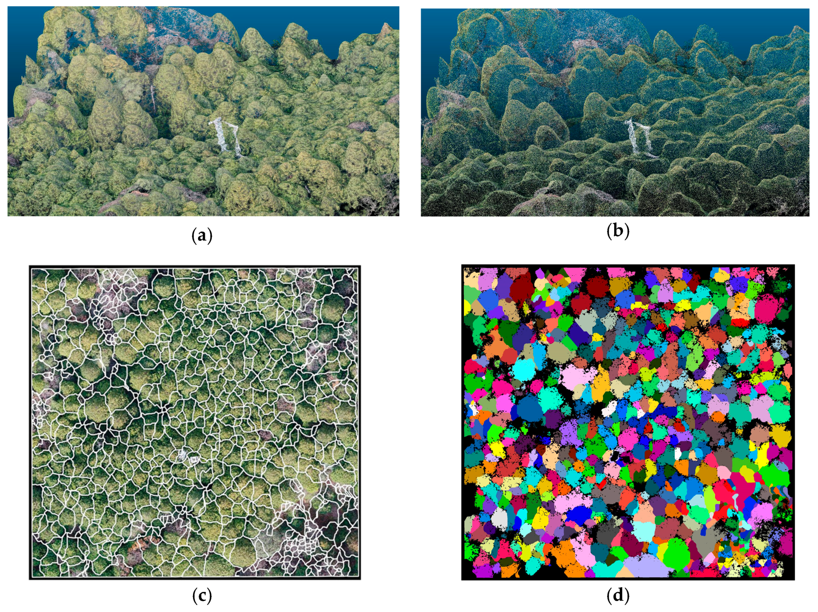
3.2. UAS Observation and Image Processing

On 19 December, 2017, a flight was conducted over the Kiryu Experimental Watershed to collect aerial photographs of the test site. A Phantom 4 Pro (DJI, Shenzhen, China) multicopter UAS was assigned an automated flight plan with DJI Ground Station (GS) Pro. The UAS took off from the top of the flux tower (approximately 29 m) and ascended an additional 70 m in altitude. The flight was designed as a grid, with the camera oriented vertically downward toward the surface, and the forward and side overlaps of each image were set to 85%. The aerial photographs collected were processed with the SfM method [46] using the Agisoft Photoscan Pro (Agisoft, St. Petersburg, Russia) ver. 1.4.2. The dense points were used to generate a digital surface model (DSM) using the inverse distance weighting (IDW) method, and the DSM was further used for orthorectification processing to generate a mosaicked image of the whole site. The original orthoimage and the DSM results have resolutions of approximately 2.3 cm and 4.6 cm, respectively (Figure 3).

3.3. Canopy Segmentation

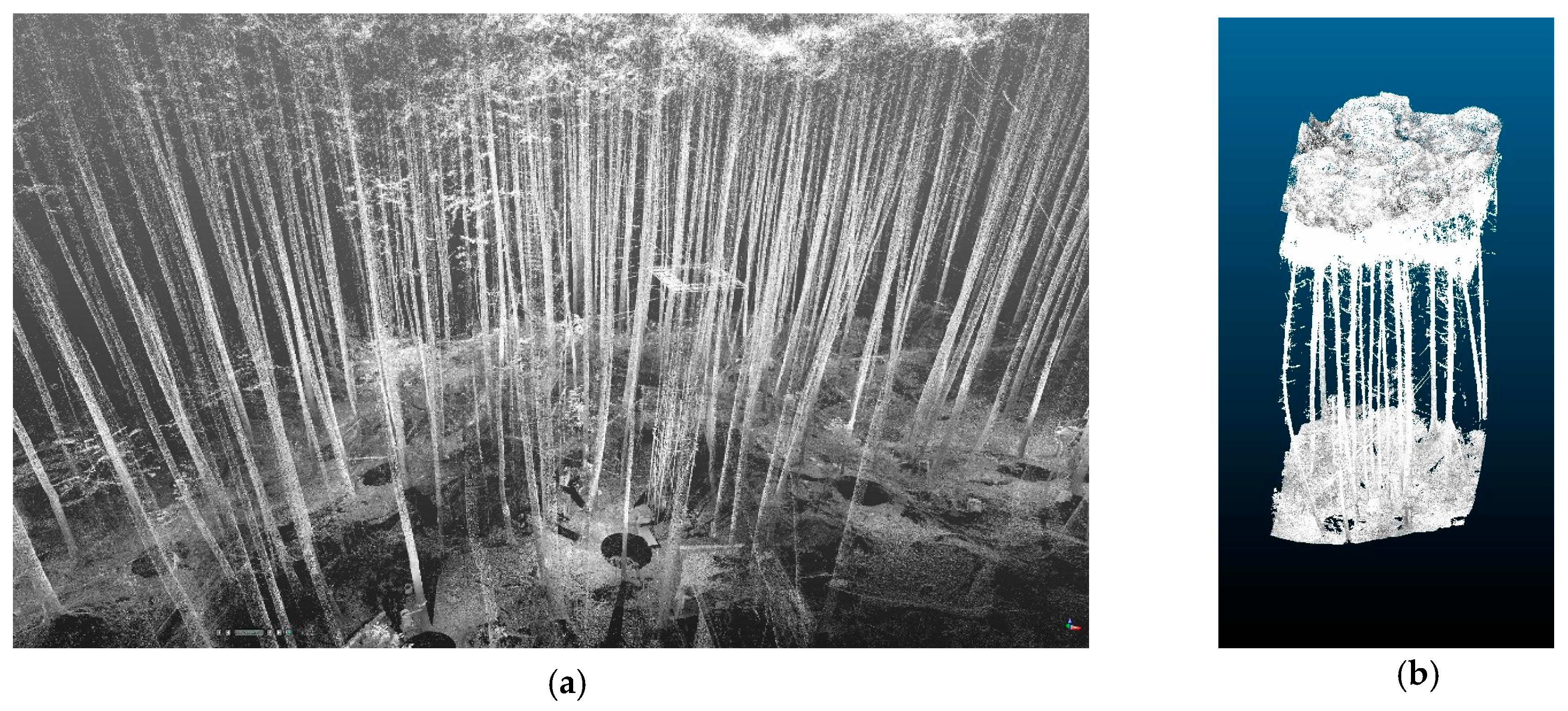
In a previous study [34], we found that the shape of the tree canopy can correlate with the diameter at breast height (DBH) and is a parameter that can be used to identify individual tree stems. The watershed segmentation [34] was implemented here to collect the individual tree canopy shapes, which could be used to estimate other forest parameters. The raw dense point cloud generated from Photoscan was imported into the CloudCompare software, an open source software for handling 3D point cloud and mesh processing [47]. The raw dense points forming the canopy shape have a bumpy, unsmoothed shape, which leads to errors when segmenting the shape of the canopy of an individual tree. Thus, in CloudCompare, the dense points were processed with a moving least squares (MLS) method in the Point Cloud Library (PCL) wrapper plugin (http://pointclouds.org/) to smooth the surface of the objects (Figure 4a,b). The smoothed alternative model was used for generating a DSM and further performed with watershed segmentation using System for Automated Geoscientific Analysis (SAGA) GIS software ver. 6.0.0 [48]. The module needed two parameters to be chosen: selected local maxima and not to assign a threshold for joining. Other parameters were left as the default values. The segmented result was overlaid with the shadow mask image, generated from the orthoimagery, to exclude areas of shadows and canopy gaps (Figure 4c,d).

3.4. TLS Survey

On 19th December, 2017, in situ measurements were carried out using TLS. A lightweight, phase-based short-range scanner (Trimble TX5, Trimble Inc., Sunnyvale, US) was used. The device uses 905 nm wavelength infrared light, and its point acquisition has the ability to measure up to 120 m in distance at a scan frequency of up to 900,000 points per second [49]. Scans were performed not only at distance intervals but also at multiple locations on the neighboring slope. For instance, one scan was collected at the bottom of the slope, while another scan was performed at the top of the neighboring slope. The scanning time was set to approximately 4 minutes, and the device rotates while scanning a 360-degree view. The scanning resolution was set to a point spacing of 12.272 mm at 10 m distance. Initial processing of the raw point cloud data and postprocessing were carried out using the Trimble RealWorks ver. 8.1 (Trimble Inc., Sunnyvale, USA). Using the cloud-based registration, the point clouds from different scanning positions were registered to each other based on the iterative closest point (ICP) algorithm to merge all points. A total of 22 scans were performed for the TLS. The merging process had an average registration accuracy of 0.6 mm for all 22 scans. Figure 5a shows an example of one of the scanning scenes.

Because the scanned TLS data are in a format of relative coordinates, the dense point cloud generated from the UAS SfM method was combined with the TLS data to determine the geocoordinates. Conventionally, ground control points (GCPs) may be used to locate the points with coordinate data, however, the densely forested area lead to difficulties in receiving sufficient GNSS (Global Navigation Satellite System) signals for use with GCPs. The flux tower was the reference object to preliminary match the top layer (SfM point cloud) and bottom layer (TLS point cloud), then the cloud to cloud registration was used same as merging the TLS scans. Registration accuracy resulted approximately 20 cm. A polygon was generated with 10 m grids, and each area was extracted (Figure 5b).

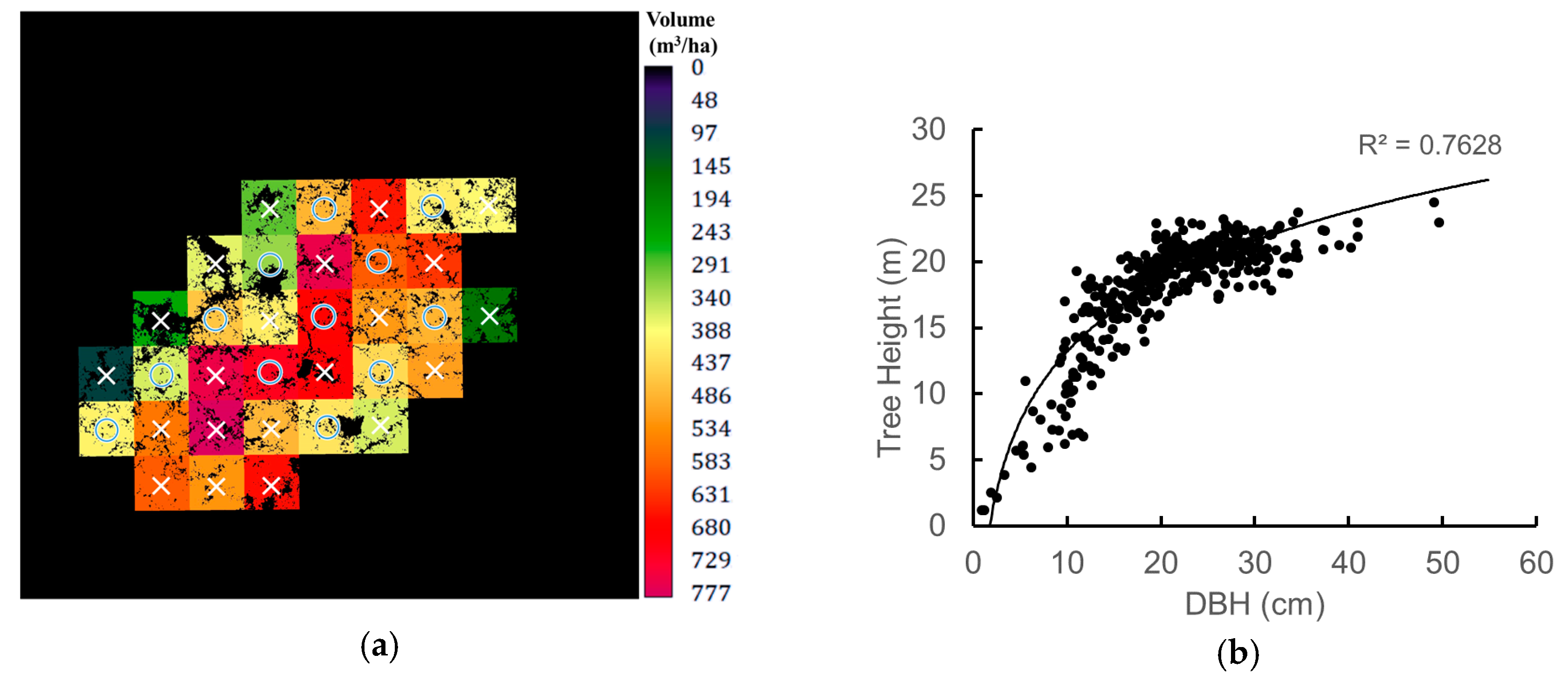
3.5. Non-Destructive Biophysical Parameter Retrieval for Ground Truth

The combined TLS point cloud was further used for measuring the forest’s biophysical parameters. Each of the plots was examined, and the tree height and the DBH were measured using the measuring tool in the RealWorks software. Tree parameters were recorded within each 10 m grid. The measured DBH and tree height data were converted into stem volume data using the Yamamoto equation [50] or the Schumacher and Hall equation [51]:

$$\log V=\mathrm{a}+\mathrm{b}\times \log D+\mathrm{c}\times \log H$$

(2)

where V is the stem volume (m³), D is DBH (cm) and H is tree height (m). The parameters a, b and c are coefficients, and for the cypress trees in this region, their values are as follows: a = −4.31101, b = 1.83546, c = 1.10655 [52]. Figure 6a,b shows the sum of the volume for each grid and the relationship between the DBH and tree height of individual trees within all grid areas. A total of 33 plots were examined, and all of the individual trees within each plot were measured. The cross and circles on Figure 6a indicate the plots further used for training (21 plots) and validation (12 plots). The total number of trees measured for all plots was n = 403. The volume data per plot was multiplied by 100 to compute the volume per unit area (m³/ha).

3.6. Generating Remotely Sensed Variables

To compute a terrain variable for the estimation, the combined point cloud data were used. The cloth simulation filter (CSF) method was implemented to extract only the terrain surface point clouds [53]. In general, the CSF method flips the 3D surface model (point cloud) upside down (inverted), and a cloth is placed on top of the surface. Depending on the use of a hard cloth or a soft cloth, the cloth surface fills the surface of the inverted 3D model. If this cloth is relatively hard (coarser resolution), the process will produce a rougher terrain surface, while a softer (finer resolution) cloth will generate topography that is more precise. By inverting back to the original axis, the cloth will form the topography of the area excluding all the top surface objects (e.g., houses, trees, etc.) (Figure 7). The parameters used for the CSF method were in steep slope mode, the cloth resolution was 0.5 m, the iteration number was 500, and the threshold was 0.2. The terrain data extracted i.e., DTM with a resolution of 3.4 mm, were then processed further to generate relative slope position (RSP) due to the heterogeneous microtopography of the test site, which might have some influence on the growth trend of the trees because of hydrological aspects [54]. A value of 1 indicates the peak of the slope, while a value of 0 indicates the bottom of the slope [55].

In total, the variables were canopy area_avg (CA_avg), canopy area_min (CA_min), canopy area_max (CA_max), CHM_avg (m), CHM_min, CHM_max, and fraction of canopy cover (FCC) (%). First, for the canopy area, the rasterized segmentation results were used as the base information. A mask image for shadows and canopy gaps was generated using the orthoimages. The mask was applied to the segmentation images to filter out areas that did not require computation. The segmentation image was processed to calculate the average, minimum and maximum value of the canopy area (in m²) within each 10 m by 10 m grid. The second variable was the tree height, expressed as the canopy height model (CHM). The DSM generated from the SfM method was used with the DTM data computed from the TLS data. By subtracting the DTM from the DSM, we obtained the height of the forested area (CHM). Additionally, the average, minimum, and maximum values of CHM were computed for each grid. Thirdly, for the FCC, the total area of canopy coverage within the grid area was computed (as a percentage).

For the radar data, γ⁰_HH, γ⁰_HV, γ⁰_VV, and γ⁰_VH backscattering intensity (dB) was prepared. Both Sentinel-1 and PALSAR have different ground resolutions of 10 m and 25 m, respectively. Therefore, to match the UAS data, both radar images were resampled to the DSMs using the cubic convolution method for further processing purposes.

3.7. Machine Learning Algorithms

RFR [56] and SVR [57] are the machine learning methods that have been used most often in image classification [58,59], and their applications have expanded to include forest attributes [60] and biomass modeling [61]. Machine learning methods are becoming an important approach in addition to traditional linear regression, because RFR and SVR can characterize the trends between the variables even when the samples are not linearly separable [62]. For the final estimation of the stem volume, two regression tests were implemented to quantify the estimation capability. The stem volume data was used as the dependent variable, while all the other remotely sensed data were used as explanatory variables. For the test, the RFR and SVR library (library “randomForest” [63] and “e1071” [64]) for the R Studio (Integrated Development for R. RStudio, Inc., Boston, MA) and the “raster” and “rgdal” packages were installed to read and process the raster images that were generated.

3.7.1. Support Vector Regression (SVR)

The type of SVR method implemented in this study was the epsilon SVR (ε-SVR). Further instruction has been provided by Mounce et al. [65] and Marabel and Alvarez-Taboada [61]. To determine the most suitable parameter, a hyperparameter optimization was performed to find the best ε, cost parameter, where ε affects the fitting of the model to the training data. A higher ε is associated with an increased error zone, which might result in fewer support vectors. The cost parameter determines the decision boundaries of data sets. A lower cost parameter allows for more errors (more general flat model), while a higher cost parameter provides tight fitting to the model (a more complex model). Training samples were collected from the “training plots” (21 plots) (indicated in Figure 6a). Stratified random sampling was used to generate 2000 samples within the area and extracted values for each variables. SVR was trained using bootstrapping sampling with a sample size of 90% and iteration = 5. A grid search method [66] was implemented to train various numbers of models with slightly different parameters. This study considered ε parameter values 0, 0.1, 0.2…1 and cost parameter values of 2², 2³, 2⁴…2⁷. More than 60 models were trained first, and from the preliminary result adjustment were made for the finer tuning of the model. The best model had values of ε = 0.01, cost = 64, as well as a radial basis function kernel, gamma = 0.1. Remaining plot area (12 plots) was used for the validation. The predicted values were averaged within the plot area and compared with the reference value.

3.7.2. Random Forest Regression (RFR)

The RFR model was developed in the same way as the procedure for SVR. The necessary parameters needed are the size of the minimum trees (node size), number of available parameters for splitting at each tree node (mtry) and the numbers of trees to grow (ntree). Again, a grid search method is used for training each models: node size = 10, 20…50; mtry = 1, 2…5; ntree = 500, 600…1500. The best model had values of node = 20, mtry = 3 and ntree = 1300. The trained model was used with the imported raster variables, and the results were computed.

3.8. Correlation of Each Variables and Validating the Predicted Models

Correlation matrix table between each of the 12 variables and stem volume were computed with Pearson’s correlation coefficients (r) and p-value for the additional check. The validation of each predicted model was considered by computing the correlation of determination (R²), root mean square error (RMSE) and relative RMSE (rRMSE) between the predicted value and the reference values. The RFR models were further tested to compute the importance of each variables, whether or not they significantly contributed to the prediction of the model. The rfPermute R-package [67] was used, which assess a null distribution of variable’s importance against the observed distribution. Each variable was shown if it was significantly different from the null distribution, considering a 5% significance level. We would like to emphasize that the R² here is considered as how well the predicted model fits to the 1:1 line, and not the proportion of the variance in the dependent variable that is predictable from the independent variable. To avoid confusion, it will be denoted as fitting R². Fitting R² was computed from the following equation:

$$R^2=1-\frac{{\displaystyle \sum }{\left(y-\widehat{y}\right)}^2}{{\displaystyle \sum }{\left(y-\overline{y}\right)}^2}$$

(3)

where y is the reference value, $\widehat{y}$ is the predicted value and $\overline{y}$ is the mean of the reference values. Alexander et al. [68] recommends the criteria of fitting R² > 0.6 indicating high correlation. Although low R² can still be plausible if the RMSE is low. However, if the model shows extreme errors then the calculations may show negative R² values; in such case it is assumed to be an erroneous model. In addition, to understand what each variable contributes, a forward stepwise selection method was applied, adding one variable at a time starting with the one that resulted in the lowest residual sum of squares. The behavior of each variable to the result is checked.

Table 1. Summary of the model combinations and its variables used. Model_1-12 is in the order from the lowest sum of residual which was checked through linear model.

Model	Variables	RFR Model	SVR Model
Model1	CHMmin	ModelRFR1	ModelSVR1
Model2	CHMavg	ModelRFR2	ModelSVR2
Model3	γ0VH	ModelRFR3	ModelSVR3
Model4	FCC	ModelRFR4	ModelSVR4
Model5	γ0VV	ModelRFR5	ModelSVR5
Model6	CAmin	ModelRFR6	ModelSVR6
Model7	CAavg	ModelRFR7	ModelSVR7
Model8	CAmax	ModelRFR8	ModelSVR8
Model9	CHMmax	ModelRFR9	ModelSVR9
Model10	γ0HV	ModelRFR10	ModelSVR10
Model11	γ0HH	ModelRFR11	ModelSVR11
Model12	RSP	ModelRFR12	ModelSVR12
Model13	Model1+2	ModelRFR13	ModelSVR13
Model14	Model1+2+3	ModelRFR14	ModelSVR14
Model15	Model1+2+3+4	ModelRFR15	ModelSVR15
Model16	Model1+2+3+4+5	ModelRFR16	ModelSVR16
Model17	Model1+2+3+4+5+6	ModelRFR17	ModelSVR17
Model18	Model1+2+3+4+5+6+7	ModelRFR18	ModelSVR18
Model19	Model1+2+3+4+5+6+7+8	ModelRFR19	ModelSVR19
Model20	Model1+2+3+4+5+6+7+8+9	ModelRFR20	ModelSVR20
Model21	Model1+2+3+4+5+6+7+8+9+10	ModelRFR21	ModelSVR21
Model22	Model1+2+3+4+5+6+7+8+9+10+11	ModelRFR22	ModelSVR22
Model23	Model1+2+3+4+5+6+7+8+9+10+11+12	ModelRFR23	ModelSVR23

summarizes the combination of the variables for each model. Furthermore, a combination of the variables were additionally modeled for three cases: minimum UAS variables (Model_UAS: CHM_avg, CA_avg and FCC), SAR only variables (Model_SAR: γ⁰_HV, γ⁰_HH, γ⁰_VV and γ⁰_VH) and both combined (Model_UAS+SAR).

4. Results

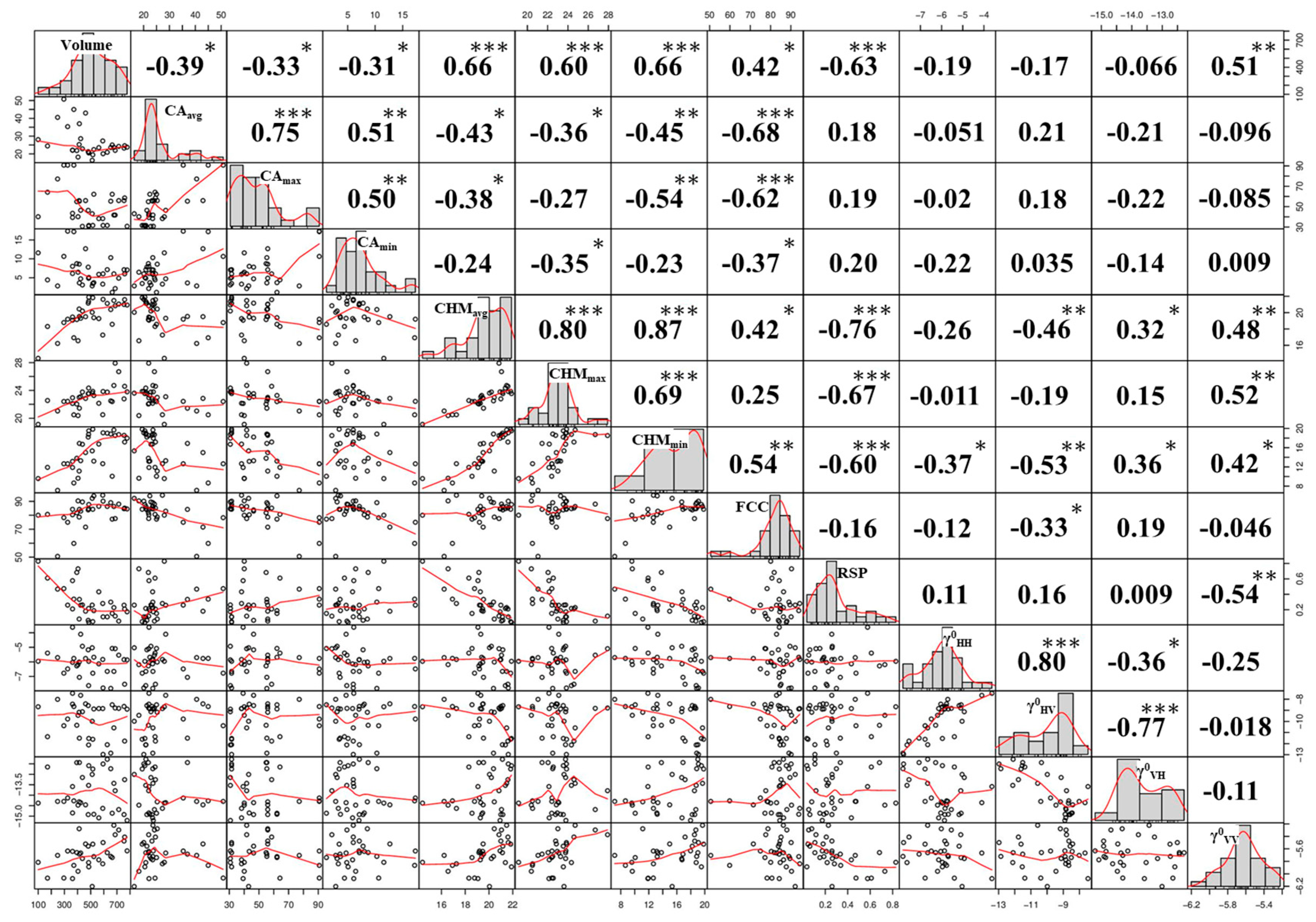
4.1. Correlation Matrix for Variable Comparison

Figure 8 presents the correlation matrix of all 13 variables. Volume was found with highest correlation for CHM_avg (r = 0.66) and CHM_min (r = 0.66), RSP (r = −0.63), CHM_max (r=0.60), followed by γ⁰_VV (r = 0.51), FCC (r = 0.42) and the CA_avg (r = −0.39). For a brief exploration of other variables correlations, CHM_min sigificantly correlated with RSP (r = −0.60), followed by FCC (r = 0.54), γ⁰_HV (r = 0.53) and other SAR variables_. The SAR variables show where γ⁰_HH correlates to CHM_min (r = −0.37), γ⁰_HV to CHM_min (r = −0.53), CHM_avg (r = −0.46) and FCC (r = −0.33). γ⁰_VH although little lower correlation, similarity is shown to γ⁰_HV. The SAR variables were not significant in their relationship to volume, except for γ⁰_VV (r = 0.51). γ⁰_VV was also correlated with RSP (r = −0.54) and CHM variables (r = 0.42−0.52). All of the SAR variables were not significant for the CA variables.

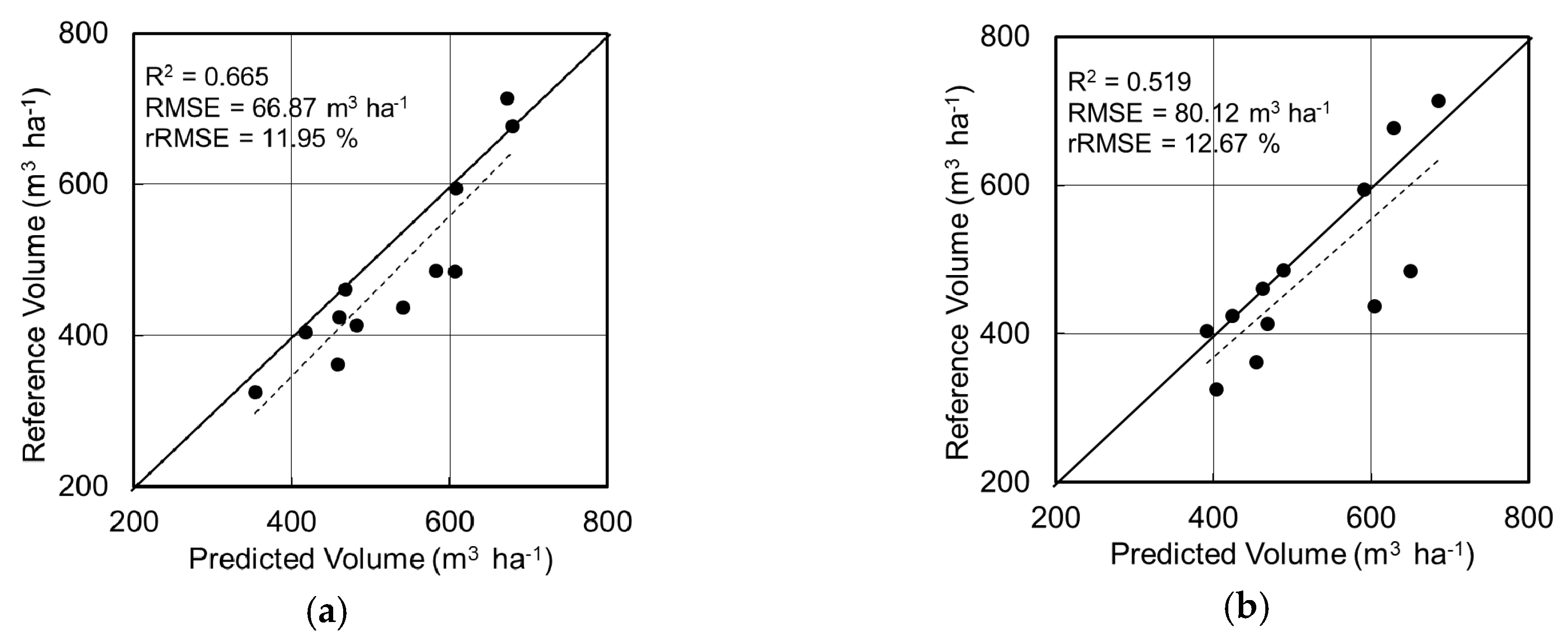
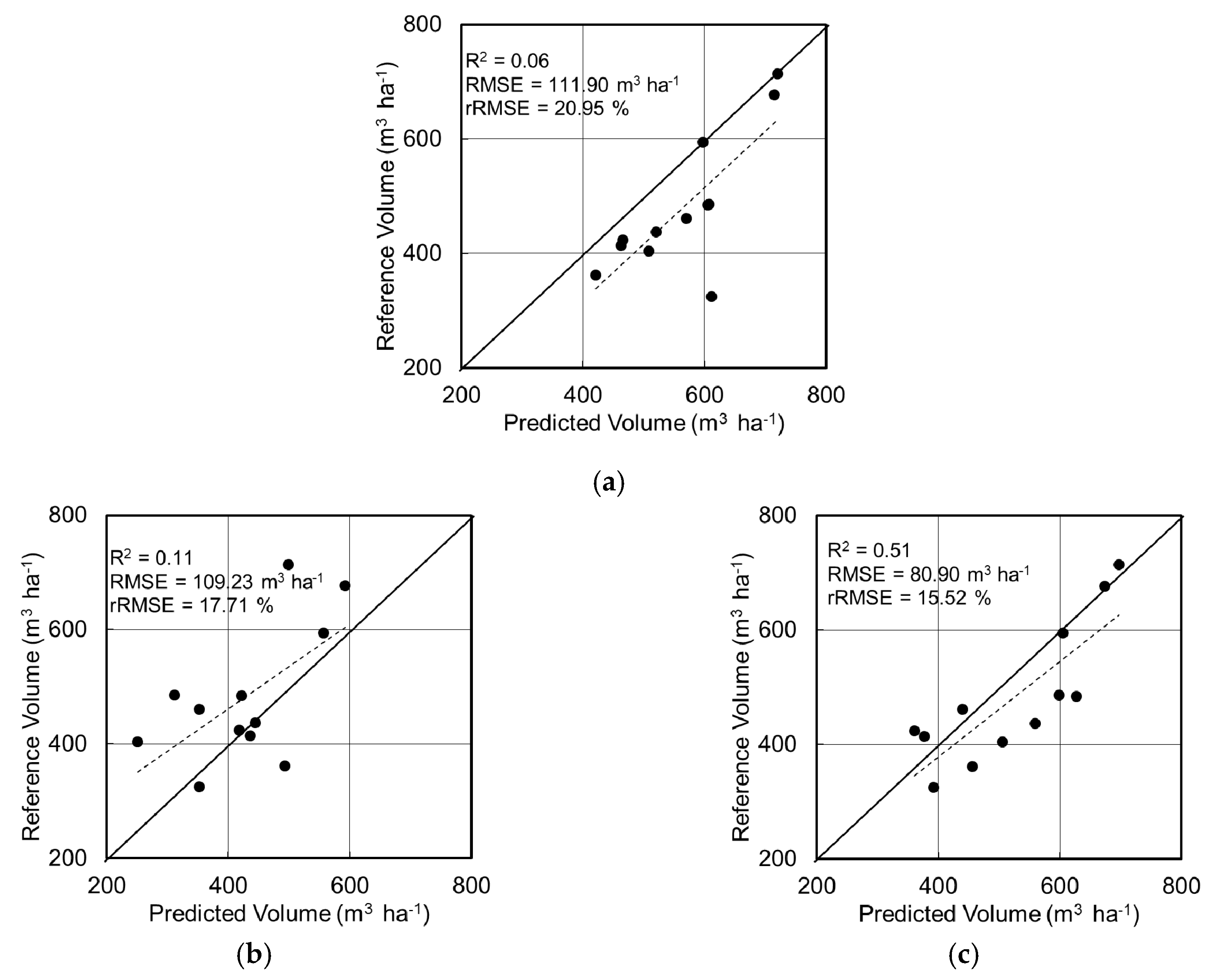
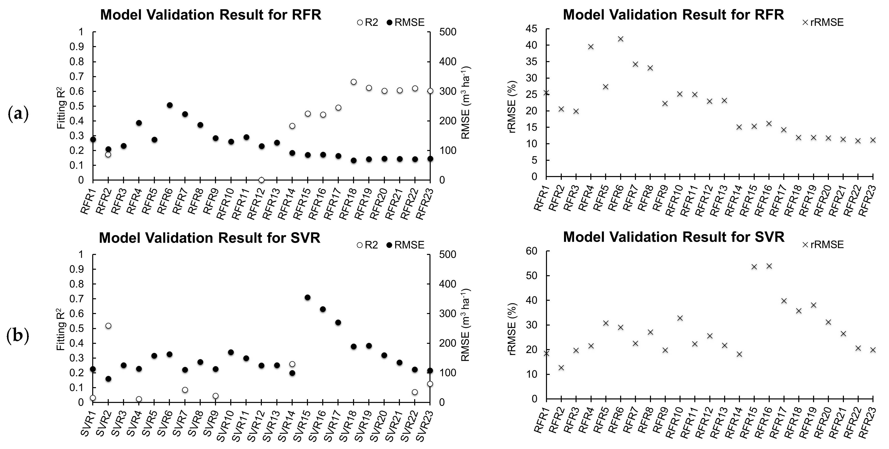
4.2. Prediction Power of RFR and SVR

Using multiple regression showed lower accuracy for SVR, and the RFR approach outperformed the SVR approach (Figure 9). Considering the numbers of models tested (Table 1), the best model for RFR was Model_RFR18 (fitting R² = 0.665, RMSE = 66.87 m³/ha, rRMSE = 11.95%), which considered CHM_min, CHM_avg, γ⁰_VH, FCC, γ⁰_VV, CA_min and CA_avg variables. The SVR method showed lower accuracy compared to RFR, where the best model was Model_SVR2 (fitting R² = 0.519, RMSE = 80.12 m³/ha, rRMSE = 12.67%), which considered CHM_avg variable. Figure 10 shows the result of the analysis with Model_UAS, Model_SAR and Model_UAS+SAR for RFR. Presentation for the SVR is omitted due to the failure of the modeling with the same variables as RFR. Model_UAS (CHM_avg, CA_avg and FCC variables) results R² = 0.06, RMSE = 111.90 m³/ha and rRMSE = 20.95%. Model_SAR results R² = 0.11, RMSE = 109.23 m³/ha and rRMSE = 17.71%. Model_UAS+SAR improves overall (R² = 0.51, RMSE = 80.90 m³/ha and rRMSE = 15.52%) and it is the only useful model compared to the former two, although majority of the validation plots were still overestimated.

Figure 11 summarizes the fitting R², RMSE, and rRMSE values of each model computed. As mentioned, a forward stepwise selection method was implemented to determine how the model behaves with the addition of each variable. For the RFR, clearly the addition of each variable enhances both the fitting R² and RMSE. The fitting R² and RMSE both showed dramatic increase in accuracy, however beyond Model₁₈, the results started to saturate. The results also show that using only the second variable (CHM_avg) can perform estimation fairly well (fitting R² = 0.173, RMSE = 105.09 m³/ha, rRMSE = 20.6%), from which we can presume that the volume is contributed more by the vertical structure (i.e., tree height). Variables related to canopy area (Model_6–8) show higher errors when used alone, which is understandable since the volume is difficult to estimate only from the horizontal information. There are differences of results for each variables, though in general it can be said that multiple regression performs better than single variable regression. SVR showed a similar trend of reducing errors in RMSE with increasing variables, although not much improvement was seen for the fitting R². The RMSE showed lower errors when all variables were combined (Model_SVR23: fitting R² = 0.126, RMSE = 108.01 m³/ha, rRMSE = 19.92%), however it achieved a better result just by using the second variable (Model_SVR2: fitting R² = 0.519, RMSE = 80.12 m³/ha, rRMSE = 12.67%). Some combinations, such as from Model_SVR15, failed to delineate the information from each variable, resulting in low fitting R² (negative value) and high RMSE and rRMSE, but gradually improve towards the full model. SVR can have better chances using the single influential variable and needs care when selecting multiple variables.

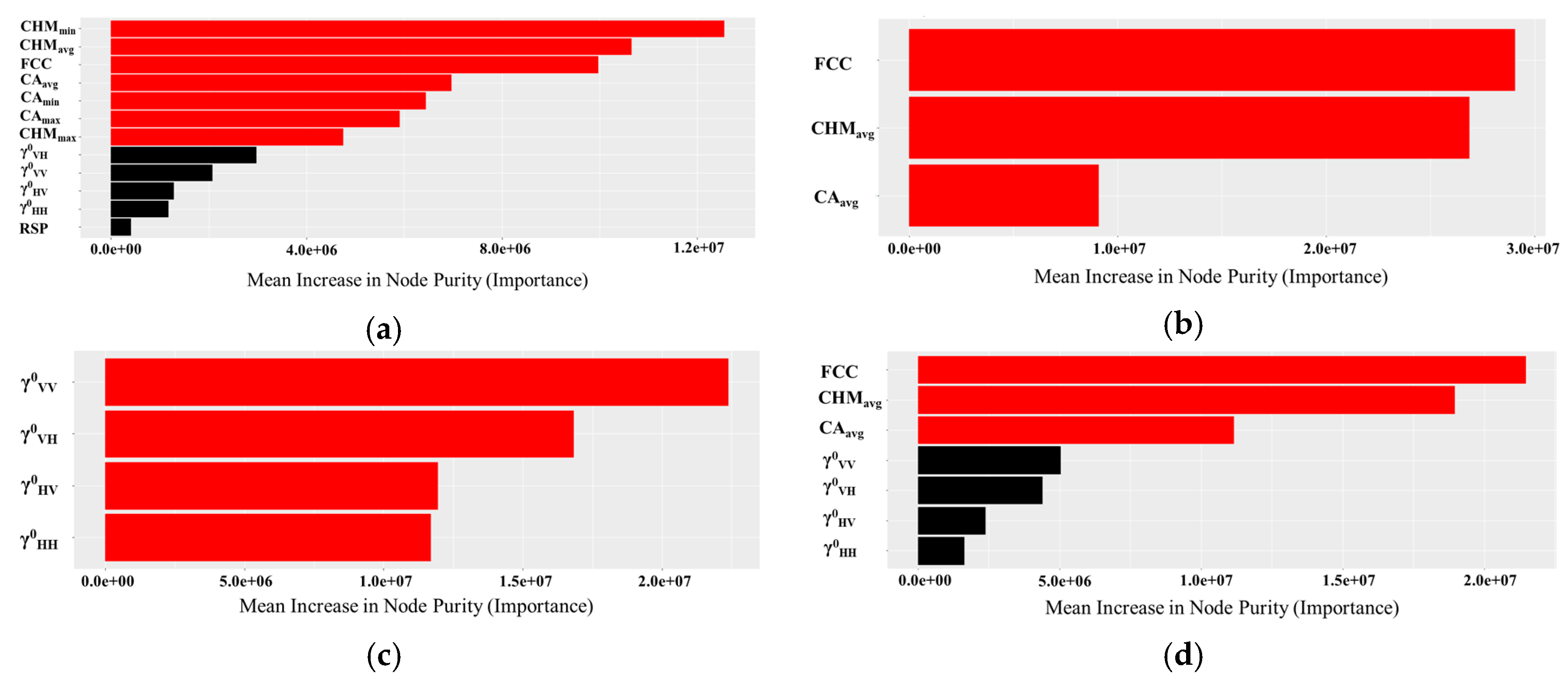
4.3. Importance and Significance of Variables (RFR)

The most important predictive variable for estimating volume (Model_RFR23) was CHM_min, shown in Figure 12 for the Gini importance measure. The variables following were CHM_avg, FCC, CA_avg, CA_min, CA_max and CHM_max, which were all indicated to be significant for partitioning the data (red bars). The additional models Model_UAS, Model_SAR, and Model_UAS+SAR are shown also. For Model_UAS+SAR, the UAS variables show that the influencing parameter for the estimation is significant, while the SAR variables, although shown to have some influence, were not significant. Using both variable sets on their own (Model_UAS and Model_SAR) showed that all the variables were significant in partitioning the data. The ranking of the Model_SAR variables changed from Model_RFR23, where γ⁰_VV influenced more than γ⁰_VH.

5. Discussion

5.1. Challenges of Multiple Regression Analysis with Multi-Sensor Data

Both the RFR and SVR methods showed good prediction of the stem volume. Our method resulted in fitting R² = 0.665, RMSE = 66.87 m³/ha (rRMSE = 11.95%) for RFR and R² = 0.519 and RMSE = 80.12 m³/ha (rRMSE = 12.67%) for SVR. They could perform better compared to the predictive power of multilinear regression (MLR) [69,70,71]; in contrast to other works, this work focused on a wide range of volumes, from approximately 100 to 800 m³/ha. If we look at a case with a stem volume range similar to that of Adbullahi et al. [71] (up to 1049 m³/ha), this work produces a better plot level estimate (although it focuses on mixed forests and the plot size is different: 500 m² circular plots) compared to using only X-band SAR data with its best accuracy of 155 m³/ha (rRMSE = 41.90%). The author discusses the possible saturation effect of the radar signals limiting the prediction. SAR saturation effects are always in discussion, and this could be caused from the large spatial unit aggregating the variations in backscattering signals (other than the limitation of radar frequency). For example, Iizuka et al. [72] tested the NDVI response to FCC with different grid resolutions. With coarser resolution, the range of the NDVI became more limited, indicating that variations were aggregated in larger units. Similar results might be shown with SAR, which limits extracting the feature information at a limiting area with lower resolution data. It was not clear in our results whether such effects were causing limitations, nevertheless, they should be noted when SAR is used in dense forest regions. This work also shows improvements compared to the works by Shataeea et al. [73] by using airborne laser scanner (ALS) and Landsat-TM data at plot level (plot size of the grid of TM data) with RF yielding 179.39 m³/ha (rRMSE = 42.93%), expressing that by adding the third dimension (i.e., tree height) data to the variable can enhance in the estimation. This was done by adding CHM information in our work. Although the ALS can produce data at a larger spatial extent, the footprints of laser scanning density may result in coarser tree information (e.g., crown delineation), although this can be overcome when utilizing UAS information. Unfortunately, similar work with the same observational scale and the integration of a multi-sensor approach was not found. Therefore, it is difficult to directly compare our results with others. Navarro et al. [40] showed the integration of UAS and Sentinel-1 and -2 for above ground biomass (AGB) estimation of mangroves in Senegal. Although it is expressed as integration, the UAS-based measurements were used as a reference for estimation with Sentinel data, and only Sentinel-1 and -2 were used. Their SVR approach using both data sets shows slightly lower validation RMSE (RMSE = 2.35 Mg/ha) compared with using only Sentinel-1 (RMSE = 2.22 Mg/ha), but improved from using only Sentinel-2 data (RMSE = 3.74 Mg/ha). Similar to our results, the multiple regression of SVR is failing. The approach of optical and SAR is possible, but needs more investigation in higher density forests.

As far as we are aware, truly integrating multi-scale/multi-resolution data has not been seen until now. For comparison, two machine learning regression was applied. The results showed that the RFR method yielded improved estimates of the stem volume compared to SVR, depending on the variables used. Validation between the reference volume showed a good fit (fitting R² = 0.665 (ΔR² = 0.146)), and the RMSE was much lower than that of the SVR approach (66.87 m³/ha (ΔRMSE = 13.25 m³/ha)). The test was conducted in a small area with few sample plots (n = 33) and with a small spatial extent. It might not compensate with broad scale analysis (unless such fine resolution data is collected broadly), however the demands of quantifying at a local scale (and extreme site dependence) might be possible from applying the proposed method. Considering the cost-effectiveness, utilizing SAR information with the aid of UAS variables of tree height and diameter would be an improvement.

5.2. Variable Selections

5.2.1. UAS Remote Sensing Variables

The variables used in this analysis were determined from the perspectives of the correlation with the volume information and the possibility of computation with a GIS platform. The canopy area has a relationship with stem DBH [34]; important information for the horizontal volume. Therefore, using this variable would have some prediction power. The same concept applies to CHM, which is a straightforward variable for tree height. Three metrics were determined for both variables: average, minimum, and maximum. Because the test samples were in a grid plot, there are variations in the canopy size and the height within the grid. Especially for canopy size, the segmentation result and the gridding in the later steps of the process removed some of the edge parts of some tree canopies, which might lead to errors in the neighboring grid where the edge of the canopy falls. The use of average, minimum, and maximum of canopy area should reduce errors, and it does show improved results when only using the average data (Figure 10). FCC provides an estimate of the gaps within the tree stands. More canopy cover means that the density is high; moreover, there are more leaves; hence, the tree height and DBH trajectory differ [74]. Therefore, depending on the FCC, DBH, and tree height, the growth characteristics and the stem volume could differ. Such information could also be obtained indirectly by giving the FCC, and is expected to improve the model; it is in fact the variable ranked third in its influence (Figure 12).

5.2.2. TLS Variables

The topographic factor, in this case, the RSP, can be considered to account for different wetness conditions in an area. Depending on the slope position, the soil water content changes, and the tree responses and processes, e.g., transpiration, differ [75]. Although the correlation matrix shows relation to volume, the addition of RSP did not result in substantial improvement in the model, but it could be used in other related works when site productivity is considered in the analysis, since wetness conditions are correlated with the growth of the cypress trees [75].

5.2.3. Radar Variables

For the radar images, studies have shown that the L-band wavelength has a stronger relationship with stems, whereas the C-band wavelength interacts more with the canopy [76,77]. The RFR and SVR model were developed by using only γ⁰_HH, γ⁰_HV, γ⁰_VV, and γ⁰_VH to estimate the volume, and the RFR resulting had moderate accuracy. The results indicate that it is possible to use the RFR approach for plot level analysis, even by using only SAR variables. Implementing SAR data is still a major candidate for global estimations for its advantages of weather and daylight independence. But it has been shown in this work that potentials can be seen for assessing local (plot-level) analysis by incorporating finer detailed information, such as from UASs. Incorporating the PALSAR and Sentinel-1 data can also produce a stronger prediction because of the incorporation of information from both the bottom and top layers of the forests [78]. Including the third variable for the forest structure (e.g., tree height) should improve its predictions. γ⁰_HH was correlated with CHM_min, γ⁰_HV and γ⁰_VH was correlated with CHM_min and CHM_avg. γ⁰_VV was the only one correlating with all CHM variables. It could be noted that C-band co-polarization response is affected more by the vertical structure of objects, and thus has a similar contribution to CHM. The cross-polarized variable usually interacts with volume, however it was not correlated significantly, and only γ⁰_VV did so. The stem volume of Chamaecyparis obtusa is influenced more by tree height, thus the γ⁰_VV correlating to all CHM variables corresponded also to volume. The complex local topography could have affected the backscattering information, which could not be as expected from other works related to L-band estimation (especially at plot level), and moreover scale difference of data resolution might have affected characterization of the local backscattering trend (brief explanation in Section 5.3). Considering the fine spatial/temporal resolution of Sentinel-1 and its availability free to the public, it can be recommended for further investigations.

5.3. Model Errors

The general issue associated with machine learning methods is always a problem such as overfitting. Extreme tight fitting of the model can fail to apply at different sites, even though the model shows a good estimation [79]. This work does not consider the application of extending the estimation to other areas, however the methodology needs further improvements and verification if forested regions need to be quantified at a broader scale. Jin et al. [79] developed a model using the random forests machine learning method to predict the tree heights for different forest types across the US using optical satellite data, topographic data, and climatic variables. They noted that training the model at one specific site and applying it to another area was not possible, whereas to some extent, better results were obtained if the model was trained using all of the samples across different sites with different vegetation types. Such a universal model improved the estimation across the US and different vegetation types. Therefore, the model in this study may not produce reliable estimates for other areas unless more training data are collected throughout the nation for a comprehensive model. Nevertheless, the prediction power of RFR was as expected and proved that it results are better than those of SVR. A key future advance would be if the RFR or the SVR method were used to develop a universal model for estimation over larger areas. Our future work will examine this potential. Possibilities include utilizing UAS LiDAR for broader and precise collection of dense point clouds while utilizing TLS for independent ground truthing of forest attributes. The combination of these two tools should enhance the methodology and produce advancements in precision forestry.

5.4. Scale Difference of Multi-Sensor Approach

Scale issues of remote sensing approaches are already taking attention and are emphasized more with advances in technology [80]. The most challenging aspect of this work is integrating platforms with various observational scales (measurement unit) [80]. The millimeter scale of TLS, centimeter scale of UAS, and 10–25 m scale of SAR can be recognized with the Modifiable Areal Unit Problem (MAUP) [81]. TLS and UAS can sense the individual tree level, while SAR data corresponding to the plot size of this study (Sentinel-1), or larger units (PALSAR-2) could have resulted with discrimination of different patterns of forest properties [82,83]. The correlation matrix showed higher correlation with Sentinel-1 and lower for PALSAR-2, and the influencing variables of model development emphasized the finer resolution Sentinel-1 VH and VV ranking higher then PALSAR-2 HH and HV data. The observational scale of the SAR data was perhaps lacking to the modeling scale [80] (10 m plot), where information of such as the aggregated PALSAR-2 data did not ensure enough features for correctly delineating the forest properties. In other words, this challenging work of multi-sensor/multi-scaled approaches could be improved with finer resolution SAR data. Navarro et al. [40] already confirms this with their estimation of UAS-based AGB with Sentinel-1 and -2 data, but in a area of sparse vegetation. Further potential uses will be investigated for densely forested areas in Japan in the future.

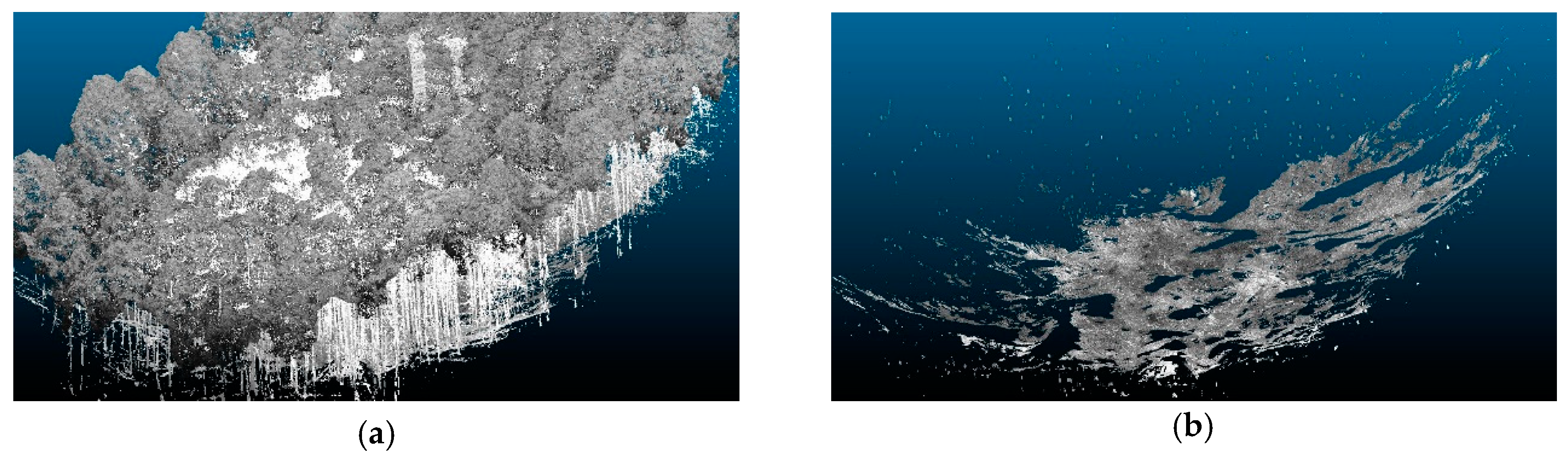
5.5. Data Processing of Point Clouds

Two issues can be discussed regarding processing and data acquisition. One is where TLS data were utilized to collect ground truth information of the stem volume of each grid area. Future challenges will increase the need for automated processes in sampling methods to increase the efficiency and consistency of measurements. The manual sampling of individual trees in dense point clouds is time consuming and requires expertise in handling the point cloud to correctly allocate each tree. However, compared with in situ observations, utilizing 3D spatial data can improve the time efficiency [84]. The motivating idea behind the collection of data with TLS was the assumption that TLS could be used to collect forest attributes as an alternative to destructive methods [27]. In fact, the sampling was successful, as evidenced by the relationship curves between DBH and tree height. No obvious outliers were found, because this study focused on a subwatershed area and the trees were correctly interpreted as evenly aged stands. The second issue was the scanning distance and the angle of the TLS. Because the returns of the laser become coarser and decrease in number with increasing distance, the structure of the canopy lacks detail. Changing the settings of the TLS to higher resolution could increase the point density [85], although there is always a tradeoff between resolution and observation time. However, the lack of canopy information makes it difficult to estimate the tree structure (tree height); hence the point cloud generated by the SfM method was used to integrate with the TLS point clouds. Points can be measured from the ground with TLS, and UAS photogrammetry can provide additional information on the tops of the canopies [86]. Moreover, the TLS data were provided with geographical coordinates because the SfM model already had coordinate information that was collected by the GNSS embedded in the UAS platform. The georeferenced results can then be combined with other data, such as satellite images. It was possible to merge the data sets at this site because the flux tower acts as a reference object in the matching of the two models; however, further consideration would be needed for other sites that lack similar reference objects.

5.6. Beyond Precision Forestry

Advances in the method for quantifying forest resources are still in progress. Even with this work’s satisfying results in improving the estimation, it will not conclude work towards this goal. In fact, goals are rather dependent on objectives. It is meaningless to follow the approach of a local scale method to analyze a global trend, or the approach of global estimation for local managements. Selecting the appropriate one is necessary, and this work contributes to advances in the approach to the local scale, possibly up to the landscape scale. Remote sensing methods can be cost effective, less time consuming and safer, compared to direct ground surveys [7]. In the case of Japan, concerns are rising concerned with reducing labor and the ageing of workers, resulting in the devastation of abandoned or unmanaged forest areas [87]. The proposed method can shed light on such issues, so that proper policies can be implemented to correctly and strategically manage the forest resources by sustainably surveying the forest with modern technologies.

6. Conclusions

This work experimented with the possibilities for estimating the plot base stem volume using random forest regression (RFR) and support vector regression (SVR), incorporating multi-sensor remote sensing data sets from TLS, UAS photogrammetry, and SAR. The RFR produced better results compared with SVR, resulting in a fitting R² = 0.665, RMSE = 66.87 m³/ha, and rRMSE =11.95%. The SVR approach showed a good correlation when a single variable was used (fitting R² = 0.519, RMSE = 80.12 m³/ha and rRMSE =12.67%), however its accuracy was reduced when multiple variables were combined (fitting R² = 0.126, RMSE = 108.01 m³/ha and rRMSE =19.92%). TLS data reveals the precise ground truth information of stem volume and terrain data. Ultra-high resolution UAS imagery has contributed to delineating forest attributes at the individual stand level, and SAR backscattering corresponded mainly with the vertical structure of the forests. The Gini index has presented the most influential variable for RFR modeling with UAS variables (canopy height, canopy size, and canopy cover), ranked by CHM_min, CHM_avg, FCC, CA_avg, CA_min, CA_max, and CHM_max. Although the case study was set in a small area, the experiment showed the potential for the incorporation of conventional remote sensing data to outperform traditional methods, utilizing only LiDAR, UAS photogrammetry, or satellite data with RFR. The proposed method could provide important information on upcoming trends in precision forestry, as various global activities need strategic actions in response to REDD+, the Paris Agreements, and the SDGs. Future challenges will be considered in the development of a comprehensive model for estimating forest parameters over broader regions and potentially at a landscape scale.

References

1. Holopainen, M.; Vastaranta, M.; Hyyppä, J. Outlook for the Next Generation’s Precision Forestry in Finland. Forests 2014, 5, 1682–1694. [Google Scholar] [CrossRef] [Green Version]
2. O’Brien, M.; Bringezu, S. Assessing the Sustainability of EU Timber Consumption Trends: Comparing Consumption Scenarios with a Safe Operating Space Scenario for Global and EU Timber Supply. Land 2017, 6, 84. [Google Scholar] [CrossRef] [Green Version]
3. Iizuka, K.; Tateishi, R. Estimation of CO2 Sequestration by the Forests in Japan by Discriminating Precise Tree Age Category using Remote Sensing Techniques. Remote Sens. 2015, 7, 15082–15113. [Google Scholar] [CrossRef] [Green Version]
4. Di Lallo, G.; Mundhenk, P.; Zamora López, S.E.; Marchetti, M.; Köhl, M. REDD+: Quick Assessment of Deforestation Risk Based on Available Data. Forests 2017, 8, 29. [Google Scholar] [CrossRef]
5. Climate Focus. Forests and Land Use in the Paris Agreement. The Paris Agreement Summary. 2015. Available online: http://www.climatefocus.com/publications/cop21-paris-2015-climate-focus-overall-summary-and-client-briefs (accessed on 20 May 2020).
6. Bastos Lima, M.G.; Kissinger, G.; Visseren-Hamakers, I.J.; Braña-Varela, J.; Gupta, A. The Sustainable Development Goals and REDD+: Assessing institutional interactions and the pursuit of synergies. Int. Environ. Agreem. 2017, 17, 589–606. [Google Scholar] [CrossRef] [Green Version]
7. Němec, P. Comparison of modern forest inventory method with the common method for management of tropical rainforest in the Peruvian Amazon. J. Trop. For. Sci. 2015, 27, 80–91. [Google Scholar]
8. Fazakas, Z.; Nilsson, M.; Olsson, H. Regional forest biomass and wood volume estimation using satellite data and ancillary data. Agric. For. Meteorol. 1999, 98–99, 417–425. [Google Scholar] [CrossRef]
9. Sandberg, G.; Ulander, L.M.H.; Fransson, J.E.S.; Holmgren, J.; Le Toan, T. L- and P-band backscatter intensity for biomass retrieval in hemiboreal forest. Remote Sens. Environ. 2011, 115, 2874–2886. [Google Scholar] [CrossRef]
10. Naidoo, L.; Mathieu, R.; Main, R.; Kleynhans, W.; Wessels, K.; Asner, G.; Leblon, B. Savannah woody structure modelling and mapping using multi-frequency (X-, C- and L-band) Synthetic Aperture Radar data. ISPRS J. Photogramm. Remote Sens. 2015, 105, 234–250. [Google Scholar] [CrossRef] [Green Version]
11. Dash, J.P.; Watt, M.S.; Bhandari, S.; Watt, P. Characterising forest structure using combinations of airborne laser scanning data, RapidEye satellite imagery and environmental variables. For. Int. J. For. Res. 2016, 89, 159–169. [Google Scholar] [CrossRef] [Green Version]
12. Barrett, F.; McRoberts, R.E.; Tomppo, E.; Cienciala, E.; Waser, L.T. A questionnaire-based review of the operational use of remotely sensed data by national forest inventories. Remote Sens. Environ. 2016, 174, 279–289. [Google Scholar] [CrossRef]
13. Saarela, S.; Grafström, A.; Ståhl, G.; Kangas, A.; Holopainen, M.; Tuominen, S.; Nordkvist, K.; Hyyppä, J. Model-assisted estimation of growing stock volume using different combinations of LiDAR and Landsat data as auxiliary information. Remote Sens. Environ. 2015, 158, 431–440. [Google Scholar] [CrossRef]
14. Goodbody, T.R.H.; Coops, N.C.; Marshall, P.L.; Tompalski, P.; Crawford, P. Unmanned aerial systems for precision forest inventory purposes: A review and case study. For. Chron. 2017, 93, 71–81. [Google Scholar] [CrossRef] [Green Version]
15. Sanga-Ngoie, K.; Iizuka, K.; Kobayashi, S. Estimating CO2 Sequestration by Forests in Oita Prefecture, Japan, by Combining LANDSAT ETM+ and ALOS Satellite Remote Sensing Data. Remote Sens. 2012, 4, 3544–3570. [Google Scholar] [CrossRef] [Green Version]
16. Vaglio Laurin, G.; Pirotti, F.; Callegari, M.; Chen, Q.; Cuozzo, G.; Lingua, E.; Notarnicola, C.; Papale, D. Potential of ALOS2 and NDVI to Estimate Forest Above-Ground Biomass, and Comparison with Lidar-Derived Estimates. Remote Sens. 2017, 9, 18. [Google Scholar] [CrossRef] [Green Version]
17. Badreldin, N.; Sanchez-Azofeifa, A. Estimating Forest Biomass Dynamics by Integrating Multi-Temporal Landsat Satellite Images with Ground and Airborne LiDAR Data in the Coal Valley Mine, Alberta, Canada. Remote Sens. 2015, 7, 2832–2849. [Google Scholar] [CrossRef] [Green Version]
18. Richards, J.A. Remote Sensing with Imaging Radar; Springer: New York, NY, USA, 2009. [Google Scholar]
19. Dobson, M.C.; Ulaby, F.T.; Le Toan, T.; Beaudoin, A.; Kasischke, E.S.; Christensen, N. Dependence of Radar Backscatter on Coniferous Forest Biomass. IEEE Trans. Geosci. Remote Sens. 1992, 30, 412–415. [Google Scholar] [CrossRef]
20. Santoro, M.; Fransson, J.E.S.; Eriksson, L.E.B.; Magnusson, M.; Ulander, L.M.H.; Olsson, H. Signatures of ALOS PALSAR L-Band Backscatter in Swedish Forest. IEEE Trans. Geosci. Remote Sens. 2009, 47, 4001–4019. [Google Scholar] [CrossRef] [Green Version]
21. Lucas, R.M.; Armston, J.; Fairfax, R.; Fensham, R.; Accad, A.; Carreiras, J.; Kelley, J.; Bunting, P.; Clewley, D.; Bray, S.; et al. An Evaluation of the ALOS PALSAR L-Band Backscatter―Above Ground Biomass Relationship Queensland, Australia: Impacts of Surface Moisture Condition and Vegetation Structure. IEEE J. Sel. Top. Appl. Earth Obs. Remote Sens. 2010, 3, 576–593. [Google Scholar] [CrossRef]
22. Motohka, T.; Shimada, M.; ISoguchi, O.; Ishihara, M.I.; Suzuki, S.N. Relationships between PALSAR Backscattering Data and Forest Above Ground Biomass in Japan. In Proceedings of the IEEE International Geoscience and Remote Sensing Symposium 2011, Vancouver, BC, Canada, 24–29 July 2011; pp. 3518–3521. [Google Scholar]
23. Kobayashi, S.; Widyorini, R.; Kawai, S.; Omura, Y.; Sanga-Ngoie, K.; Supriadi, B. Backscattering Characteristics of L-Band Polarimetric and Optical Satellite Imagery over Planted Acacia Forests in Sumatra, Indonesia. J. Appl. Remote Sens. 2012, 6, 063519–063525. [Google Scholar]
24. Iizuka, K.; Tateishi, R. Simple Relationship Analysis between L-Band Backscattering Intensity and the Stand Characteristics of Sugi (Cryptomeria japonica) and Hinoki (Chamaecyparis obtusa) Trees. Adv. Remote Sens. 2014, 3, 219–234. [Google Scholar] [CrossRef] [Green Version]
25. Srinivasan, S.; Popescu, S.C.; Eriksson, M.; Sheridan, R.D.; Ku, N.-W. Terrestrial Laser Scanning as an Effective Tool to Retrieve Tree Level Height, Crown Width, and Stem Diameter. Remote Sens. 2015, 7, 1877–1896. [Google Scholar] [CrossRef] [Green Version]
26. Hayakawa, Y.S.; Kusumoto, S.; Matta, N. Application of terrestrial laser scanning for detection of ground surface deformation in small mud volcano (Murono, Japan). Earth Planets Space 2016, 68, 114. [Google Scholar] [CrossRef] [Green Version]
27. Momo Takoudjou, S.; Ploton, P.; Sonké, B.; Hackenberg, J.; Griffon, S.; De Coligny, F.; Kamdem, N.G.; Libalah, M.; Mofack, G.I.; Le Moguédec, G.; et al. Using terrestrial laser scanning data to estimate large tropical trees biomass and calibrate allometric models: A comparison with traditional destructive approach. Methods Ecol. Evol. 2018, 9, 905–916. [Google Scholar]
28. Flynn, K.F.; Chapra, S.C. Remote Sensing of Submerged Aquatic Vegetation in a Shallow Non-Turbid River Using an Unmanned Aerial Vehicle. Remote Sens. 2014, 6, 12815–12836. [Google Scholar] [CrossRef] [Green Version]
29. Getzin, S.; Nuske, R.S.; Wiegand, K. Using Unmanned Aerial Vehicles (UAV) to Quantify Spatial Gap Patterns in Forests. Remote Sens. 2014, 6, 6988–7004. [Google Scholar] [CrossRef] [Green Version]
30. Luna, I.; Lobo, A. Mapping Crop Planting Quality in Sugarcane from UAV Imagery: A Pilot Study in Nicaragua. Remote Sens. 2016, 8, 500. [Google Scholar] [CrossRef] [Green Version]
31. Ota, T.; Ogawa, M.; Shimizu, K.; Kajisa, T.; Mizoue, N.; Yoshida, S.; Takao, G.; Hirata, Y.; Furuya, N.; Sano, T.; et al. Aboveground Biomass Estimation Using Structure from Motion Approach with Aerial Photographs in a Seasonal Tropical Forest. Forests 2015, 6, 3882–3898. [Google Scholar] [CrossRef] [Green Version]
32. Jucker, T.; Caspersen, J.; Chave, J.; Antin, C.; Barbier, N.; Bongers, F.; Dalponte, M.; van Ewijk, K.Y.; Forrester, D.I.; Haeni, M.; et al. Allometric equations for integrating remote sensing imagery into forest monitoring programmes. Glob. Chang. Biol. 2017, 23, 177–190. [Google Scholar] [CrossRef]
33. Panagiotidis, D.; Abdollahnejad, A.; Surový, P.; Chiteculo, V. Determining tree height and crown diameter from high-resolution UAV imagery. Int. J. Remote Sens. 2017, 38, 2392–2410. [Google Scholar] [CrossRef]
34. Iizuka, K.; Yonehara, T.; Itoh, M.; Kosugi, Y. Estimating Tree Height and Diameter at Breast Height (DBH) from Digital Surface Models and Orthophotos Obtained with an Unmanned Aerial System for a Japanese Cypress (Chamaecyparis obtusa). For. Remote Sens. 2018, 10, 13. [Google Scholar] [CrossRef] [Green Version]
35. Jaakkola, A.; Hyyppä, J.; Yu, X.; Kukko, A.; Kaartinen, H.; Liang, X.; Hyyppä, H.; Wang, Y. Autonomous Collection of Forest Field Reference—The Outlook and a First Step with UAV Laser Scanning. Remote Sens. 2017, 9, 785. [Google Scholar] [CrossRef] [Green Version]
36. Schlund, M.; Davidson, M.W.J. Aboveground Forest Biomass Estimation Combining L- and P-Band SAR Acquisitions. Remote Sens. 2018, 10, 1151. [Google Scholar] [CrossRef] [Green Version]
37. Shao, Z.; Zhang, L. Estimating Forest Aboveground Biomass by Combining Optical and SAR Data: A Case Study in Genhe, Inner Mongolia, China. Sensors 2016, 16, 834. [Google Scholar] [CrossRef] [Green Version]
38. Cutler, M.; Boyd, D.; Foody, G.; Vetrivel, A. Estimating tropical forest biomass with a combination of SAR image texture and Landsat TM data: An assessment of predictions between regions. ISPRS J. Photogramm. Remote Sens. 2012, 70, 66–77. [Google Scholar] [CrossRef] [Green Version]
39. Karlson, M.; Ostwald, M.; Reese, H.; Sanou, J.; Tankoano, B.; Mattsson, E. Mapping Tree Canopy Cover and Aboveground Biomass in Sudano-Sahelian Woodlands Using Landsat 8 and Random Forest. Remote Sens. 2015, 7, 10017–10041. [Google Scholar] [CrossRef] [Green Version]
40. Navarro, J.A.; Algeet, N.; Fernández-Landa, A.; Esteban, J.; Rodríguez-Noriega, P.; Guillén-Climent, M.L. Integration of UAV, Sentinel-1, and Sentinel-2 Data for Mangrove Plantation Aboveground Biomass Monitoring in Senegal. Remote Sens. 2019, 11, 77. [Google Scholar] [CrossRef] [Green Version]
41. Kosugi, Y.; Takanashi, S.; Ueyama, M.; Ohkubo, S.; Tanaka, H.; Matsumoto, K.; Yoshifuji, N.; Ataka, M.; Sakabe, A. Determination of the gas exchange phenology in an evergreen coniferous forest from 7 years of eddy covariance flux data using an extended big-leaf analysis. Ecol. Res. 2013, 28, 373–385. [Google Scholar] [CrossRef]
42. Japan Aerospace Exploration Agency (JAXA). PALSAR Calibration Factor Updated. Available online: http://www.eorc.jaxa.jp/en/about/distribution/info/alos/20090109en_3.html (accessed on 12 June 2018).
43. Small, D. Flattening gamma: Radiometric terrain correction for SAR imagery. IEEE Trans. Geosci. Remote Sens. 2011, 49, 3081–3093. [Google Scholar] [CrossRef]
44. Omar, H.; Misman, M.A.; Kassim, A.R. Synergetic of PALSAR-2 and Sentinel-1A SAR Polarimetry for Retrieving Aboveground Biomass in Dipterocarp Forest of Malaysia. Appl. Sci. 2017, 7, 675. [Google Scholar] [CrossRef] [Green Version]
45. Lee, J.S. Speckle suppression and analysis for synthetic aperture radar images. Opt. Eng. 1986, 25, 636–643. [Google Scholar] [CrossRef]
46. Mlambo, R.; Woodhouse, I.H.; Gerard, F.; Anderson, K. Structure from Motion (SfM) Photogrammetry with Drone Data: A Low Cost Method for Monitoring Greenhouse Gas Emissions from Forests in Developing Countries. Forests 2017, 8, 68. [Google Scholar] [CrossRef] [Green Version]
47. Girardeau-Montaut, D. CloudCompare. Available online: http://www.cloudcompare.org/ (accessed on 13 June 2018).
48. Conrad, O.; Bechtel, B.; Bock, M.; Dietrich, H.; Fischer, E.; Gerlitz, L.; Wehberg, J.; Wichmann, V.; Böhner, J. System for Automated Geoscientific Analyses (SAGA) v. 2.1.4. Geosci. Model Dev. 2015, 8, 1991–2007. [Google Scholar] [CrossRef] [Green Version]
49. Trimble Navigation Limited (2012) Datasheet Trimble TX5 Scanner. Available online: http://www.trimble.com/globalTRL.asp?nav=Collection-91149 (accessed on 2 July 2018).
50. Yamamoto, W. Forest inventory of Japanese red pine for stem volume and diameter at breast height (あかまつノ単木幹材積表並胸高形数表). Bull. For. Exp. 1918, 16, 147–164. (In Japanese) [Google Scholar]
51. Schumacher, F.X.; Hall, F.D.S. Logarithmic expression of timber-tree volume. J. Agric. Res. 1933, 47, 719–734. [Google Scholar]
52. Hosoda, K.; Mitsuda, Y.; Iehara, T. Differences between the present stem volume tables and the values of the volume equations, and their correction. Jpn. Soc. For. Plan. 2010, 44, 23–39. (In Japanese) [Google Scholar]
53. Zhang, W.; Qi, J.; Wan, P.; Wang, H.; Xie, D.; Wang, X.; Yan, G. An Easy-to-Use Airborne LiDAR Data Filtering Method Based on Cloth Simulation. Remote Sens. 2016, 8, 501. [Google Scholar] [CrossRef]
54. Adams, H.R.; Barnard, H.R.; Loomis, A.K. Topography alters tree growth–climate relationships in a semi-arid forested catchment. Ecosphere 2014, 5, 148. [Google Scholar] [CrossRef]
55. MacMillan, R.A.; Pettapiece, W.W.; Nolan, S.C.; Goddard, T.W. A generic procedure for automatically segmenting landforms into landform elements using DEMs, heuristic rules and fuzzy logic. Fuzzy Sets Syst. 2000, 113, 81–109. [Google Scholar] [CrossRef]
56. Breiman, L. Random Forests. Mach. Learn. 2001, 45, 5–32. [Google Scholar] [CrossRef] [Green Version]
57. Boser, B.E.; Guyon, I.M.; Vapnik, V.N. A Training Algorithm for Optimal Margin Classifiers. In Proceedings of the 5th Annual Workshop on Computational Learning Theory (COLT’92), Pittsburgh, PA, USA, 27–29 July 1992; pp. 144–152. [Google Scholar]
58. Shao, Y.; Lunetta, R.S. Comparison of support vector machine, neural network, and CART algorithms for the land-cover classification using limited training data points. ISPRS J. Photogramm. Remote Sens. 2012, 70, 78–87. [Google Scholar] [CrossRef]
59. Negri, R.G.; Dutra, L.V.; Sant’Anna, S.J.S. An innovative support vector machine based method for contextual image classification. ISPRS J. Photogramm. Remote Sens. 2014, 87, 241–248. [Google Scholar] [CrossRef]
60. Wu, J.; Yao, W.; Choi, S.; Park, T.; Myneni, R.B. A Comparative Study of Predicting DBH and Stem Volume of Individual Trees in a Temperate Forest Using Airborne Waveform LiDAR. IEEE Geosci. Remote Sens. Lett. 2015, 12, 2267–2271. [Google Scholar] [CrossRef]
61. Marabel, M.; Alvarez-Taboada, F. Spectroscopic Determination of Aboveground Biomass in Grasslands Using Spectral Transformations, Support Vector Machine and Partial Least Squares Regression. Sensors 2013, 13, 10027–10051. [Google Scholar] [CrossRef] [PubMed] [Green Version]
62. Gao, Y.; Lu, D.; Li, G.; Wang, G.; Chen, Q.; Liu, L.; Li, D. Comparative Analysis of Modeling Algorithms for Forest Aboveground Biomass Estimation in a Subtropical Region. Remote Sens. 2018, 10, 627. [Google Scholar] [CrossRef] [Green Version]
63. Liaw, A.; Wiener, M. Classification and Regression by randomForest. R News 2002, 2, 18–22. [Google Scholar]
64. Meyer, D.; Dimitriadou, E.; Hornik, K.; Weingessel, A.; Leisch, F. e1071: Misc Functions of the Department of Statistics, Probability Theory Group (Formerly: E1071), TU Wien. R Package Version 1.7-3. 2019. Available online: https://CRAN.R-project.org/package=e1071 (accessed on 20 May 2020).
65. Mounce, S.R.; Mounce, R.B.; Boxall, J.B. Novelty detection for time series data analysis in water distribution systems using support vector machines. J. Hydroinform. 2011, 13, 672–686. [Google Scholar] [CrossRef]
66. García, M.; Riaño, D.; Chuvieco, E.; Salas, J.F.; Danson, M. Multispectral and LiDAR data fusion for fuel type mapping using Support Vector Machine and decision rules. Remote Sens. Environ. 2011, 115, 1369–1379. [Google Scholar] [CrossRef]
67. Archer, E. rfPermute: Estimate Permutation p-Values for Random Forest Importance Metrics. R Package Version 2.1.81. 2020. Available online: https://CRAN.R-project.org/package=rfPermute (accessed on 20 May 2020).
68. Alexander, D.L.J.; Tropsha, A.; Winkler, D.A. Beware of R2: Simplee, unambiguous assessment of the prediction accuracy of QSAR and QSPR models. J. Chem. Inf. Model. 2015, 55, 1316–1322. [Google Scholar] [CrossRef] [Green Version]
69. Lindberg, E.; Hollaus, M. Comparison of Methods for Estimation of Stem Volume, Stem Number and Basal Area from Airborne Laser Scanning Data in a Hemi-Boreal Forest. Remote Sens. 2012, 4, 1004–1023. [Google Scholar] [CrossRef] [Green Version]
70. He, Q.; Chen, E.; An, R.; Li, Y. Above-Ground Biomass and Biomass Components Estimation Using LiDAR Data in a Coniferous Forest. Forests 2013, 4, 984–1002. [Google Scholar] [CrossRef] [Green Version]
71. Abdullahi, S.; Kugler, F.; Pretzsch, H. Prediction of stem volume in complex temperate forest stands using TanDEM-X SAR data. Remote Sens. Environ. 2016, 174, 197–211. [Google Scholar] [CrossRef]
72. Iizuka, K.; Kato, T.; Silsigia, S.; Soufiningrum, A.Y.; Kozan, O. Estimating and Examining the Sensitivity of Different Vegetation Indices to Fractions of Vegetation Cover at Different Scaling Grids for Early Stage Acacia Plantation Forests Using a Fixed-Wing UAS. Remote Sens. 2019, 11, 1816. [Google Scholar] [CrossRef] [Green Version]
73. Shataeea, S.; Weinaker, H.; Babanejad, M. Plot-level Forest Volume Estimation Using Airborne Laser Scanner and TM Data, Comparison of Boosting and Random Forest Tree Regression Algorithms. Procedia Environ. Sci. 2011, 7, 68–73. [Google Scholar] [CrossRef] [Green Version]
74. Sumida, A.; Miyaura, T.; Toori, H. Relationships of tree height and diameter at breast height revisited: Analyses of stem growth using 20-year data of an even-aged Chamaecyparis obtusa stand. Tree Physiol. 2013, 33, 106–118. [Google Scholar] [CrossRef] [PubMed]
75. Nagakura, J.; Shigenaga, H.; Akama, A.; Takahashi, M. Growth and transpiration of Japanese cedar (Cryptomeria japonica) and Hinoki cypress (Chamaecyparis obtusa) seedlings in response to soil water content. Tree Physiol. 2004, 23, 1203–1208. [Google Scholar] [CrossRef]
76. Kobayashi, S.; Omura, Y.; Sanga-Ngoie, K.; Widyorini, R.; Kawai, S.; Supriadi, B.; Yamaguchi, Y. Characteristics of Decomposition Powers of L-Band Multi-Polarimetric SAR in Assessing Tree Growth of Industrial Plantation Forests in the Tropics. Remote Sens. 2012, 4, 3058–3077. [Google Scholar] [CrossRef] [Green Version]
77. Varghese, A.O.; Suryavanshi, A.; Joshi, A.K. Analysis of different polarimetric target decomposition methods in forest density classification using C band SAR data. Int. J. Remote Sens. 2016, 37, 694–709. [Google Scholar] [CrossRef]
78. Sivasankar, T.; Lone, J.M.; Sarma, K.K.; Qadir, A.; Raju, P.L.N. The potential of multi-frequency multipolarized ALOS-2/PALSAR-2 and Sentinel-1 SAR data for aboveground forest biomass estimation. Int. J. Eng. Technol. 2018, 10, 797–802. [Google Scholar] [CrossRef] [Green Version]
79. Jin, S.; Su, Y.; Gao, S.; Hu, T.; Liu, J.; Guo, Q. The Transferability of Random Forest in Canopy Height Estimation from Multi-Source Remote Sensing Data. Remote Sens. 2018, 10, 1183. [Google Scholar] [CrossRef] [Green Version]
80. Wu, H.; Li, Z.-L. Scale Issues in Remote Sensing: A Review on Analysis, Processing and Modeling. Sensors 2009, 9, 1768–1793. [Google Scholar] [CrossRef] [PubMed]
81. Jelinski, D.E.; Wu, J. The modifiable areal unit problem and implications for landscape ecology. Landsc. Ecol. 1996, 11, 129–140. [Google Scholar] [CrossRef]
82. Ulander, L.M.H.; Smith, G.; Eriksson, L.; Folkesson, K.; Fransson, J.E.S.; Gustavsson, A.; Hallberg, B.; Joyce, S.; Magnusson, M.; Olsson, H.; et al. Mapping of wind-thrown forests in southern Sweden using space- and airborne SAR. In Proceedings of the International Geoscience and Remote Sensing Symposium (IGARSS), Seoul, Korea, 25–29 July 2005; pp. 3619–3622. [Google Scholar]
83. Carrer, M.; Castagneri, D.; Popa, I.; Pividori, M.; Lingua, E. Tree spatial patterns and stand attributes in temperate forests: The importance of plot size, sampling design, and null model. For. Ecol. Manag. 2018, 407, 125–134. [Google Scholar] [CrossRef]
84. Saarinen, N.; Kankare, V.; Vastaranta, M.; Luoma, V.; Pyörälä, J.; Tanhuanpää, T.; Liang, X.; Kaartinen, H.; Kukko, A.; Jaakkola, A.; et al. Feasibility of Terrestrial laser scanning for collecting stem volume information from single trees. ISPRS J. Photogramm. Remote Sens. 2017, 123, 140–158. [Google Scholar] [CrossRef]
85. Roşca, S.; Suomalainen, J.; Bartholomeus, H.; Herold, M. Comparing terrestrial laser scanning and unmanned aerial vehicle structure from motion to assess top of canopy structure in tropical forests. Interface Focus 2018, 8, 20170038. [Google Scholar] [CrossRef] [PubMed]
86. Tian, J.; Dai, T.; Li, H.; Liao, C.; Teng, W.; Hu, Q.; Ma, W.; Xu, Y. A Novel Tree Height Extraction Approach for Individual Trees by Combining TLS and UAV Image-Based Point Cloud Integration. Forests 2019, 10, 537. [Google Scholar] [CrossRef] [Green Version]
87. Forestry Agency, Japan. State of Japan’s Forests and Forest Management. 2019. Available online: https://www.maff.go.jp/e/policies/forestry/attach/pdf/index-8.pdf (accessed on 16 May 2020).
Figure 1. Characteristics of the Kiryu Experimental Watershed. Moderately dense trees are seen at the site with heterogeneous microtopography. The middle image shows the flux tower at the site from the surface, and the right image shows the flux tower and the surrounding landscape as seen from the unmanned aerial system (UAS) (Photo by author: 19 December, 2017). Detail of geographical location is shown by Iizuka et al. [34].
Remotesensing 12 01649 g001
Figure 2. Flowchart of the methodology. Terrestrial laser scanning (TLS) was used for ground truthing and generation of the digital terrain model (DTM). A UAS was utilized for collecting aerial images, which were then processed to obtain a digital surface model (DSM) and orthoimages. Phased Array type L-band Synthetic Aperture Radar-2 (PALSAR-2) and Sentinel-1 data were preprocessed and used as independent variables. All variables were incorporated in the end with different regression analysis for the test.
Remotesensing 12 01649 g002
Figure 3. (a) Orthoimage of the study site, and (b) DSM generated from the aerial imageries and the structure from motion (SfM) method. 345 images taken from the flight, the SfM method was successfully applied to the site.
Remotesensing 12 01649 g003
Figure 4. (a) Full dense point cloud of the study site and (b) smoothed point cloud processed with the moving least squares (MLS) method. (c) The polygons generated from the smoothed point cloud using the watershed segmentation, and (d) the final canopy shape from masking the canopy gaps and shadows. Random colors represent the canopy shapes, while black is the background (gap and shadows).
Remotesensing 12 01649 g004
Figure 5. (a) Merged TLS scans of the study site, and (b) example of the extracted sample area with the 10 by 10 m grid size. Each individual tree was measured to compute tree height and diameter at breast height (DBH) within the grids.
Remotesensing 12 01649 g005
Figure 6. (a) Total stem volume per grid (m3/ha) and (b) the tree height–DBH relationship curve for the trees within the sample grids (n = 403). Shadow and canopy gaps are masked out in the raster image. The crosses and circles on each grids indicates the plot area used for training (21 plots) and validation (12 plots), respectively.
Remotesensing 12 01649 g006
Figure 7. Dense point cloud of the merged UAS SfM points and TLS points of the study site (a) before the CSF filter and (b) after the filtering. The CSF successfully excluded the top surface objects (e.g., trees, the tower, etc.) and left only the surface terrain.
Remotesensing 12 01649 g007
Figure 8. Correlation matrix with significant levels between stem volume and other 12 variables. Diagonal matrices show the histogram of the data distribution. The left half is the bivariate scatter plot with fitted line. The right half shows the Pearson correlation and the significance level associated with a symbol: p-values < 0.001 (***), < 0.01 (**), < 0.05 (*).
Remotesensing 12 01649 g008
Figure 9. Model validation results from the regression analysis. Comparison of the reference and predicted stem volumes at each validation plots (indicated in Figure 6a) for (a) random forest regression (RFR) and (b) support vector regression (SVR). The figure shows the best result from the modelling. RFR = ModelRFR18; SVR = ModelSVR2. The solid black line indicates the 1:1 line. The dotted line is the linear trend line between the predicted and reference volume just for the visual reference, and it does not represent the R2 shown.
Remotesensing 12 01649 g009
Figure 10. Results from the RFR analysis. Comparison of the reference and predicted stem volumes for additional models using, (a) minimum UAS variables (CHMavg, CAavg, FCC) (b) SAR variables, and (c) UAS+SAR variables. The solid black line indicates the 1:1 line. The dotted line is the linear trend line between the predicted and reference volume just for the visual reference, and it does not represent the R2 shown.
Remotesensing 12 01649 g010
Figure 11. Summary of the results for all regression analyses tested. Each result for the correlation of determination (R2), root mean square error (RMSE), and relative RMSE (rRMSE) is shown for (a) RFR and (b) SVR. Only positive R2 is drawn and the models and without R2 plots indicates all negative fitting R2, hence erroneous models.
Remotesensing 12 01649 g011
Figure 12. Importance of each variables explained as the mean increase in node purity (i.e., decrease in node impurity: Gini Index) for (a) ModelRFR23, (b) ModelUAS, (c) ModelSAR, and (d) ModelUAS+SAR. The upper shows more influential variables used in the random forest model for estimating stem volume. Red color bars indicates the parameter that significantly partitioned the data.
Remotesensing 12 01649 g012