Monitoring Agricultural Fields Using Sentinel-1 and Temperature Data in Peru: Case Study of Asparagus (Asparagus officinalis L.)


Abstract
:
1. Introduction
1.1. Related Work
1.2. Objectives of the Study
- To analyse the SAR response to the asparagus crop evolution.
- To present examples of how the seasonal climatological conditions influence the crop development in the test site (tropical conditions).
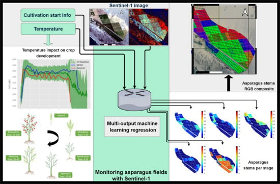
- To present the implementation of a data-driven methodology that captures the recurrent patterns in the SAR response and the temperature to provide an approximation of the crop development at every new SAR acquisition. It consists of a Multi-output machine learning regression algorithm in which each output estimates the number of asparagus stems that are present in each of the predefined phenological stages at a given date.
2. Materials and Methods
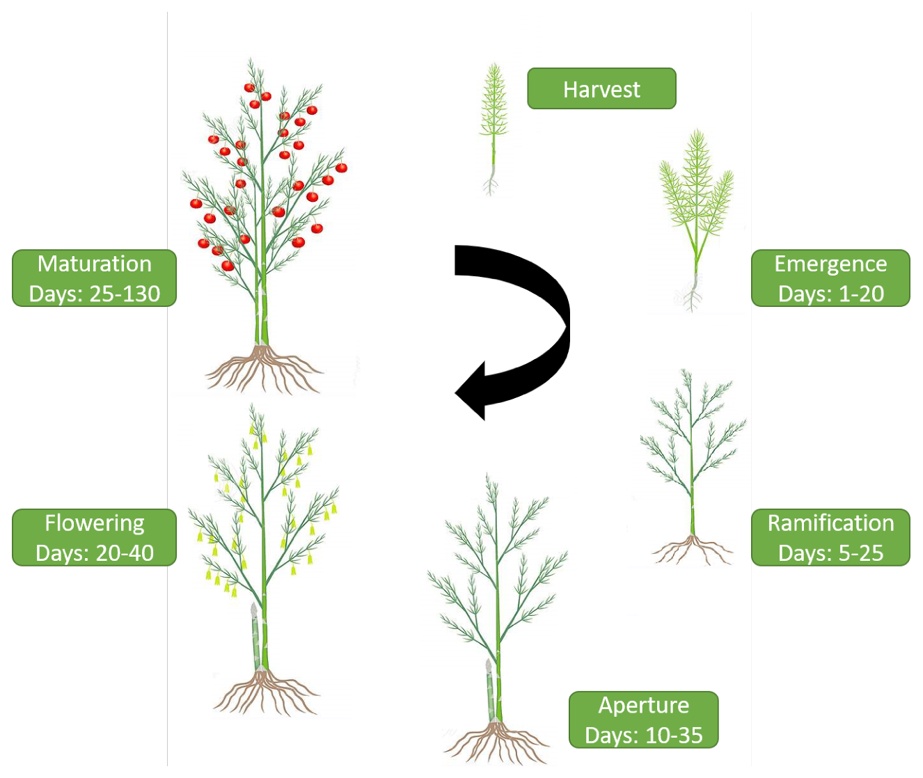
2.1. Asparagus Crop Development and Production Cycles
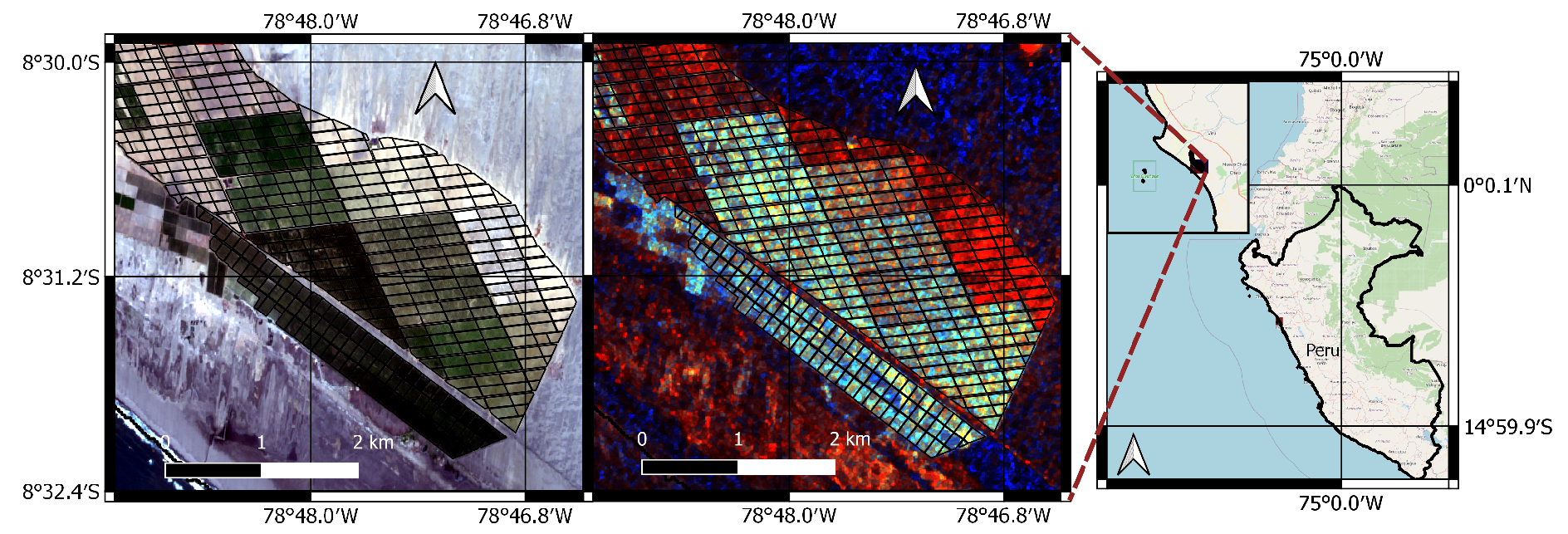
2.2. Test Site
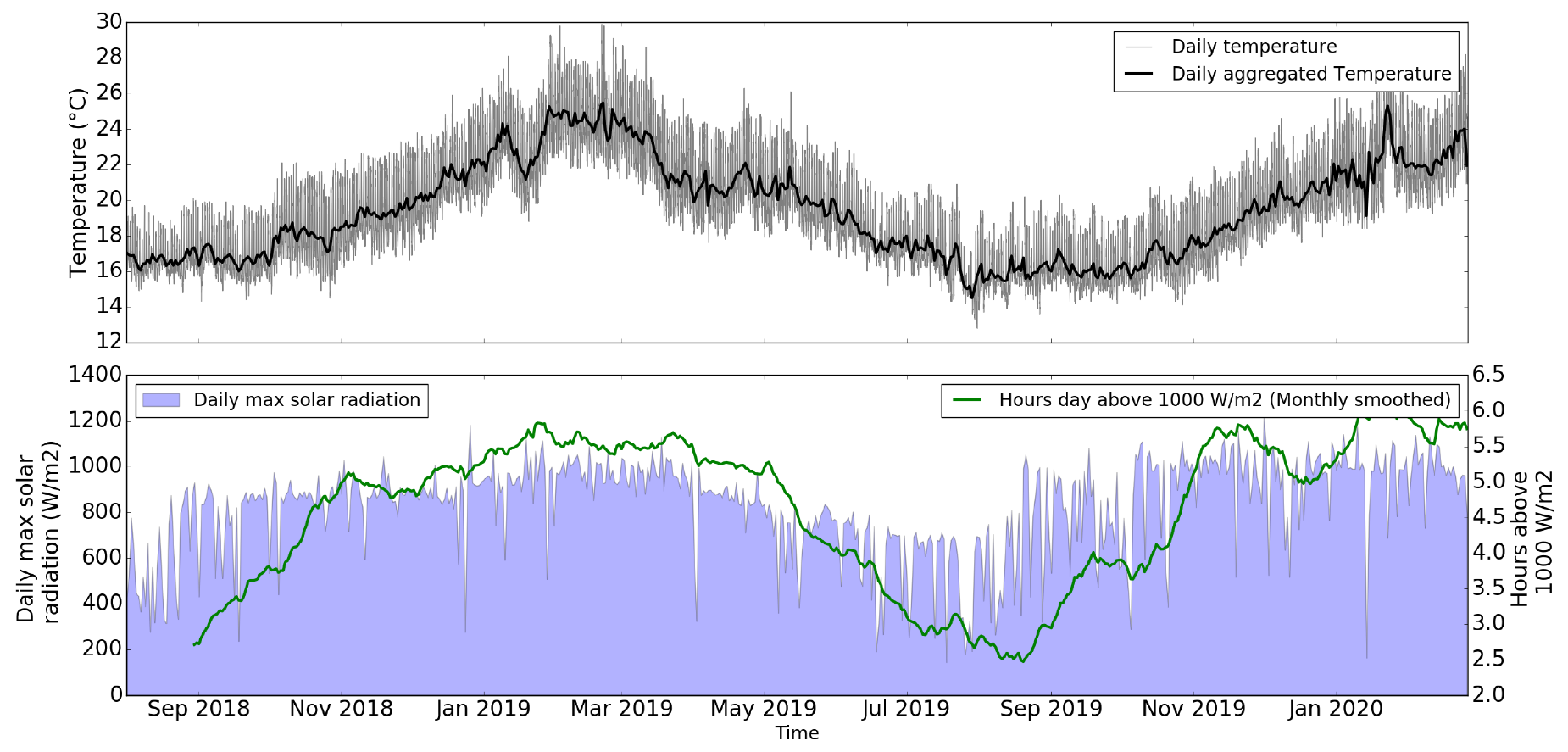
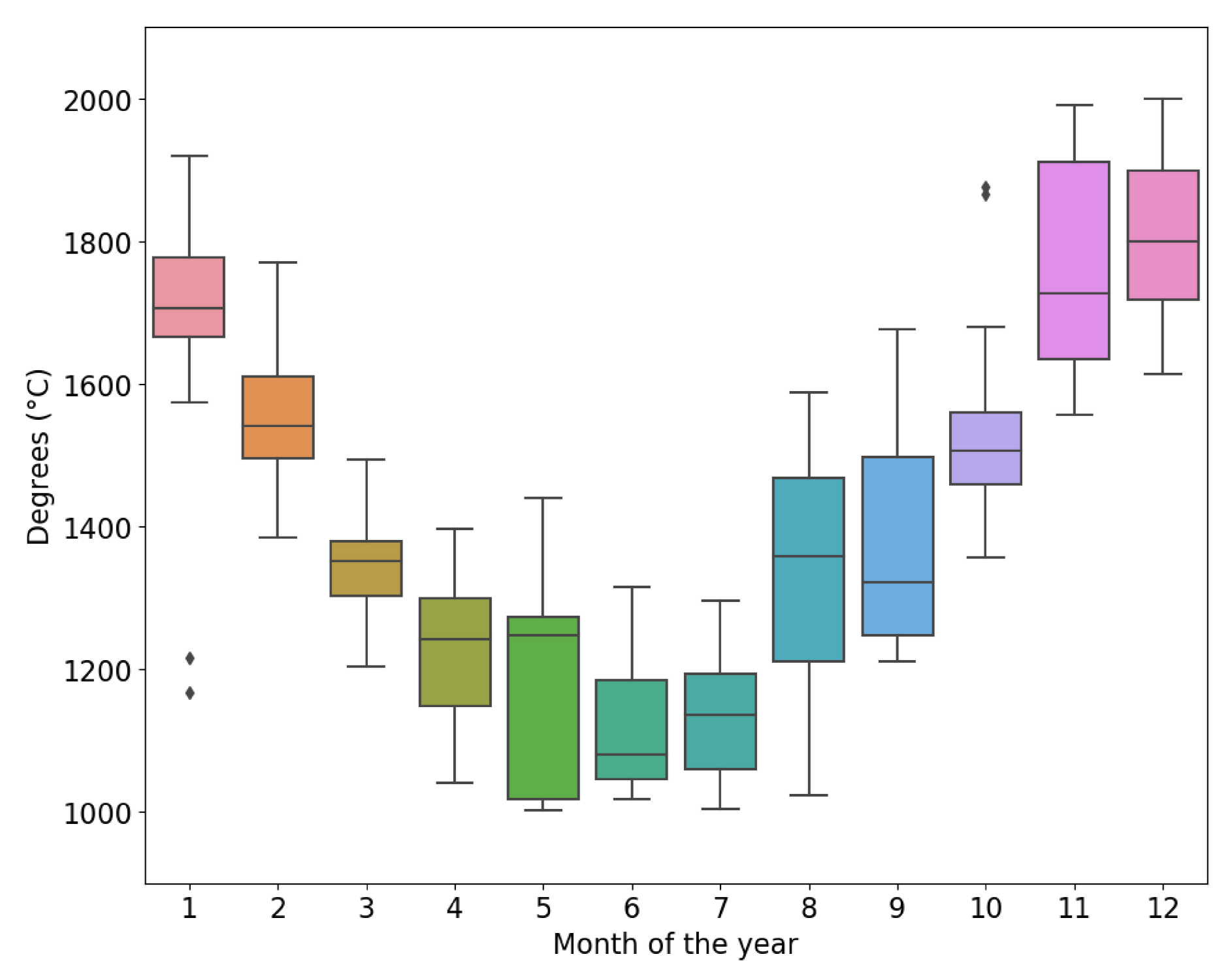
2.3. Climatological Conditions
2.4. Ground Truth
2.5. Sar Datasets
2.6. Methodology for Estimating Asparagus Stems Per Stage
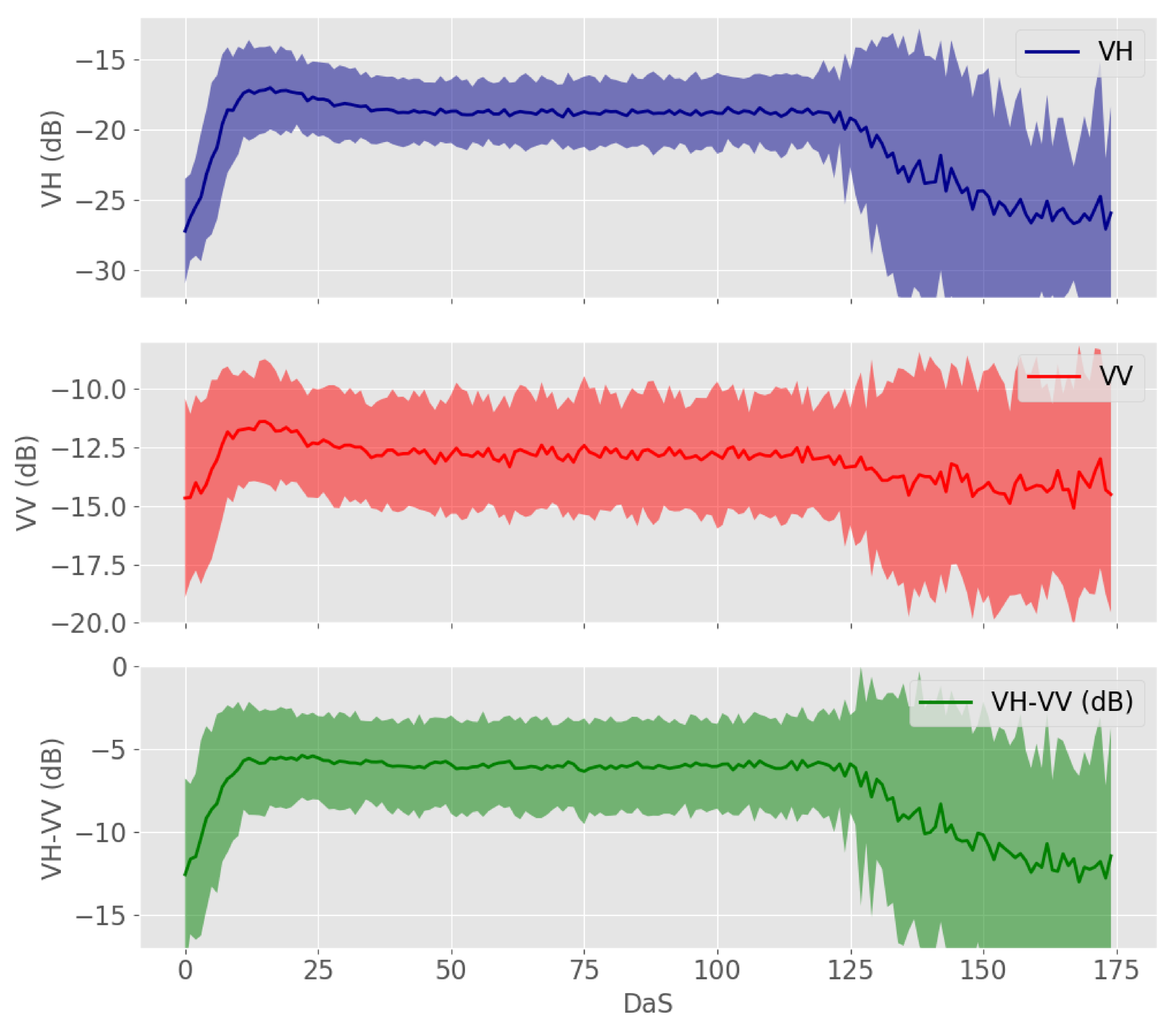
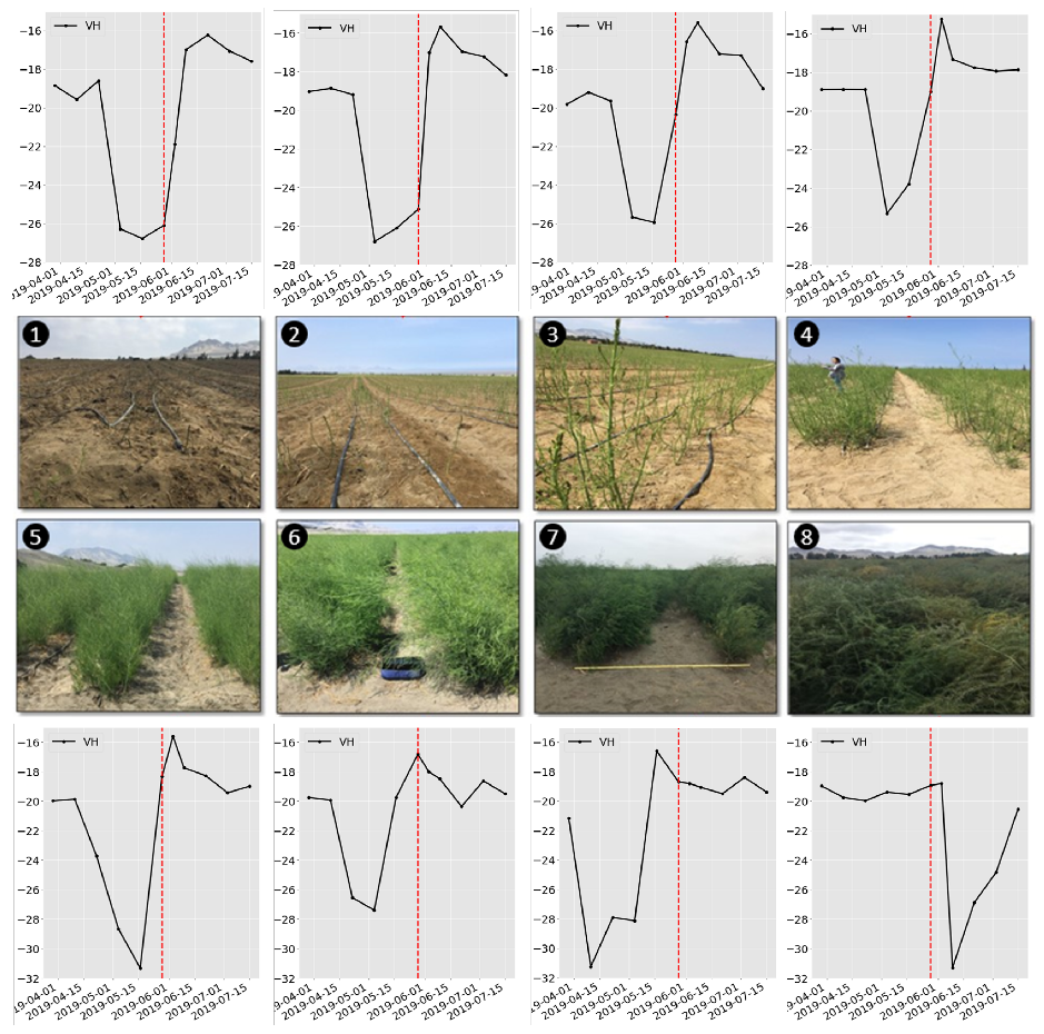
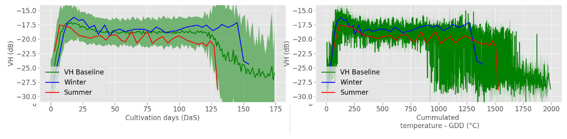
2.6.1. Sar Sensitivity to Crop Evolution
2.6.2. Impact of Temperature on the Crop and the Sar Response
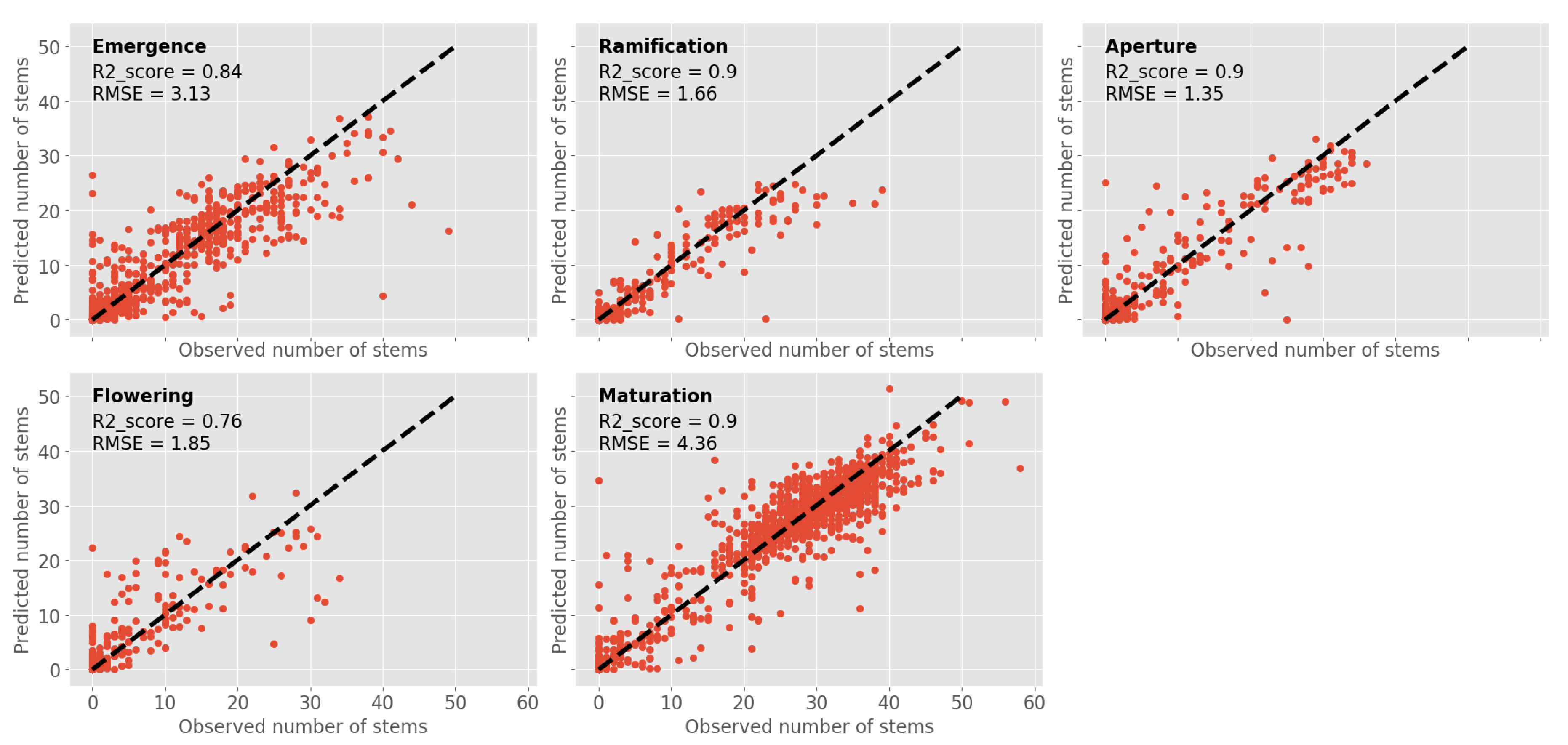
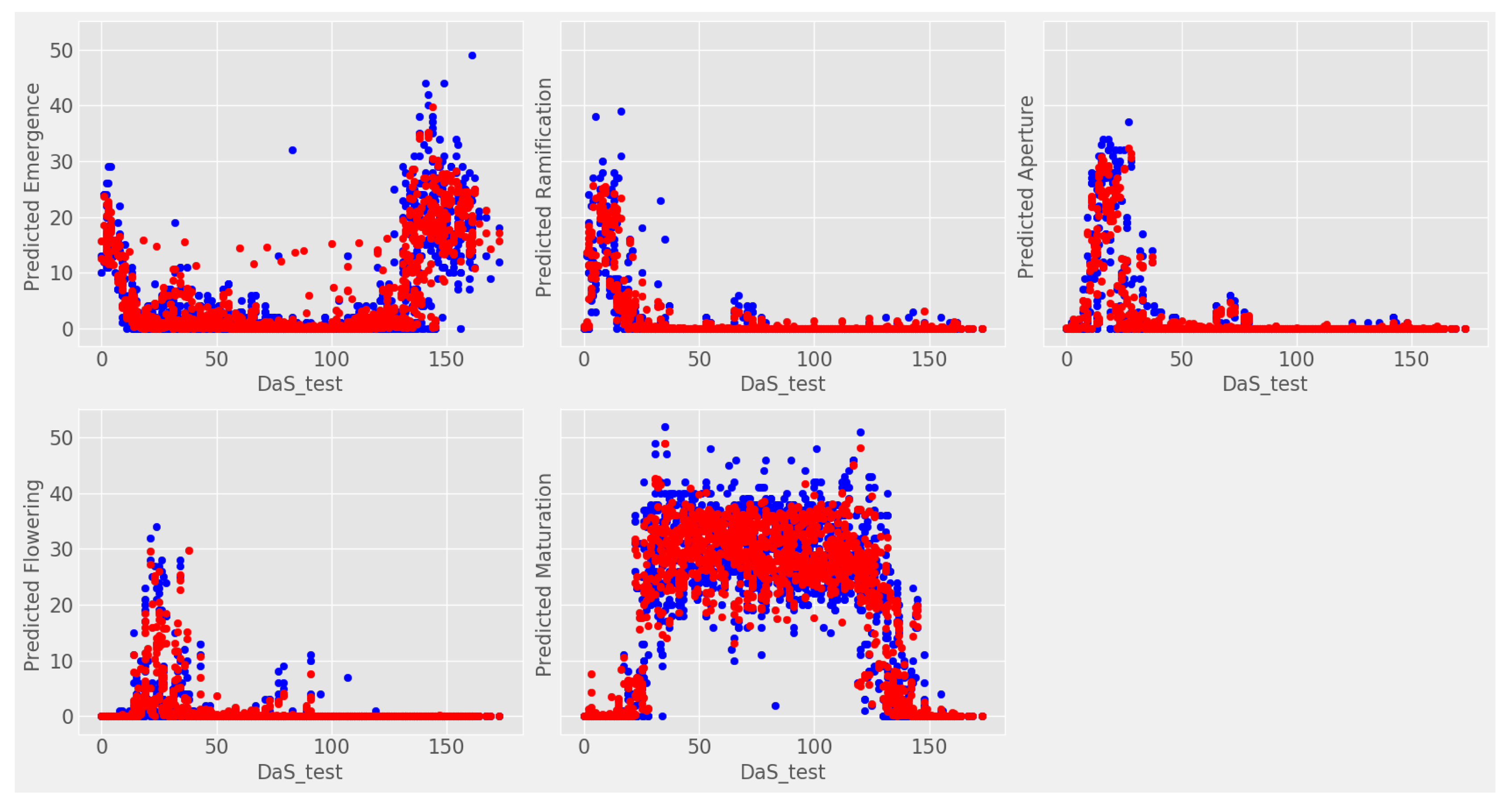
2.7. Estimation of Number of Asparagus Stems in Each Crop Stage
2.7.1. Model Development
2.7.2. Inputs
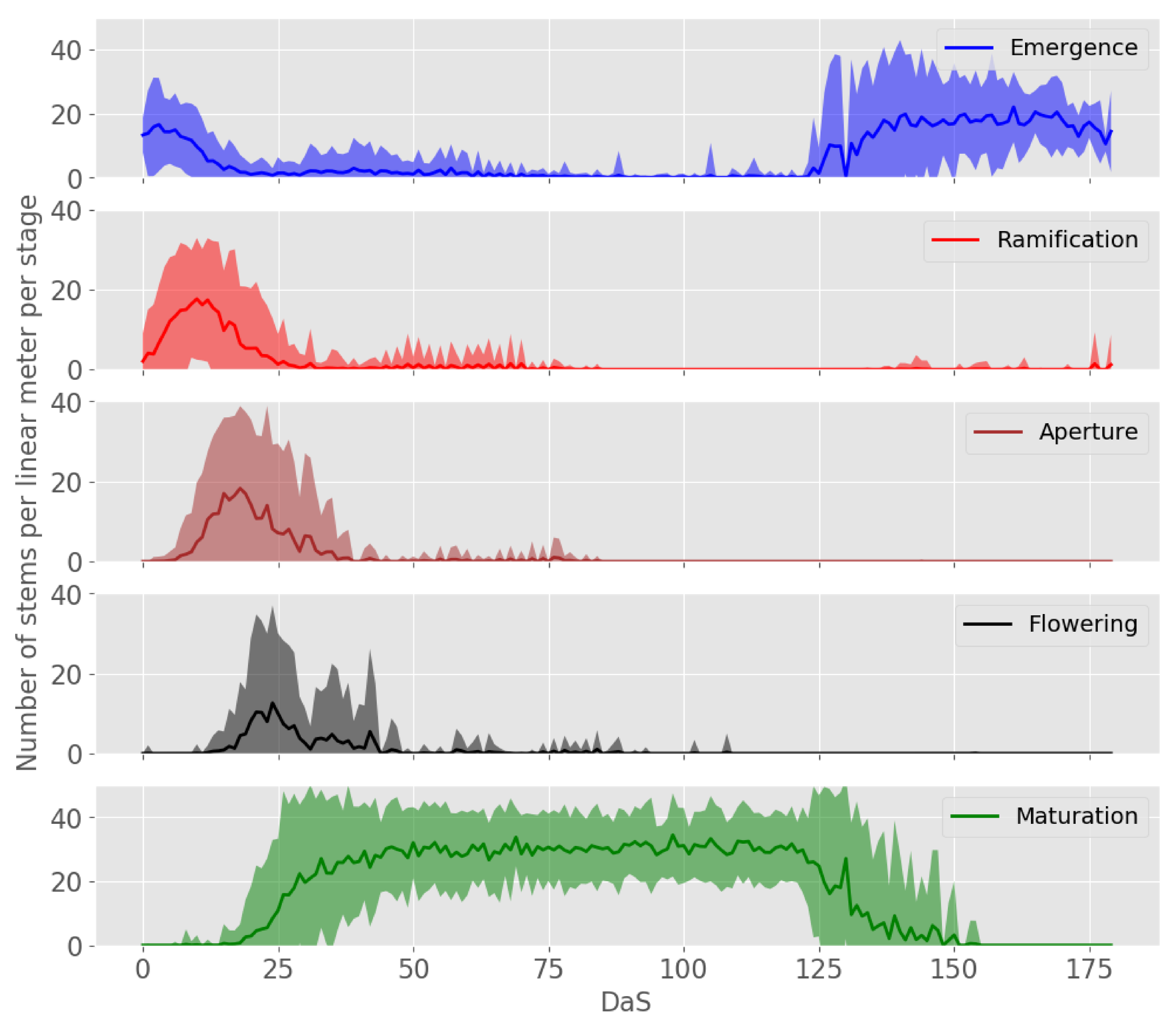
2.7.3. Outputs
2.7.4. Training and Testing Data
2.7.5. Model Hyper Parameters
2.7.6. Accuracy Metrics
3. Results
3.1. Single-Sar Image Results
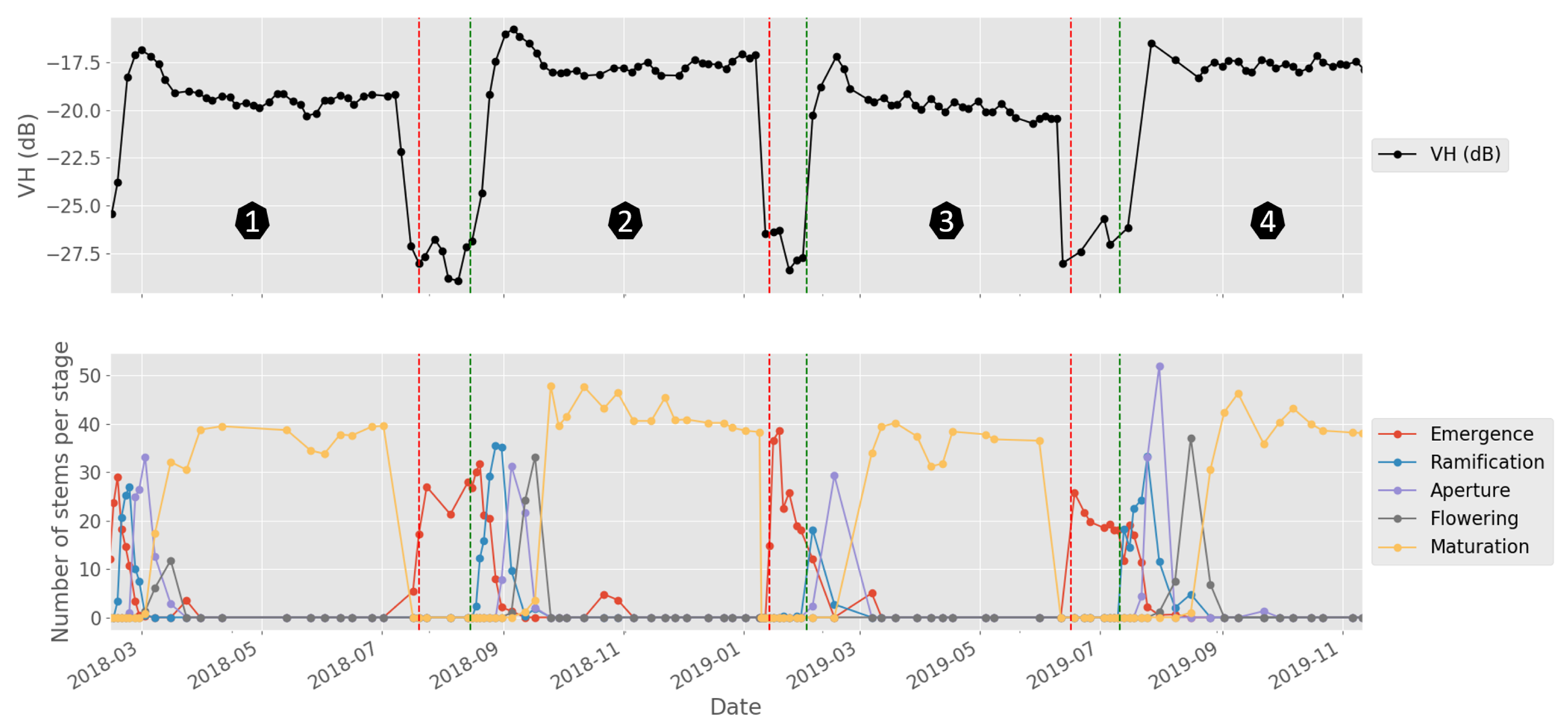
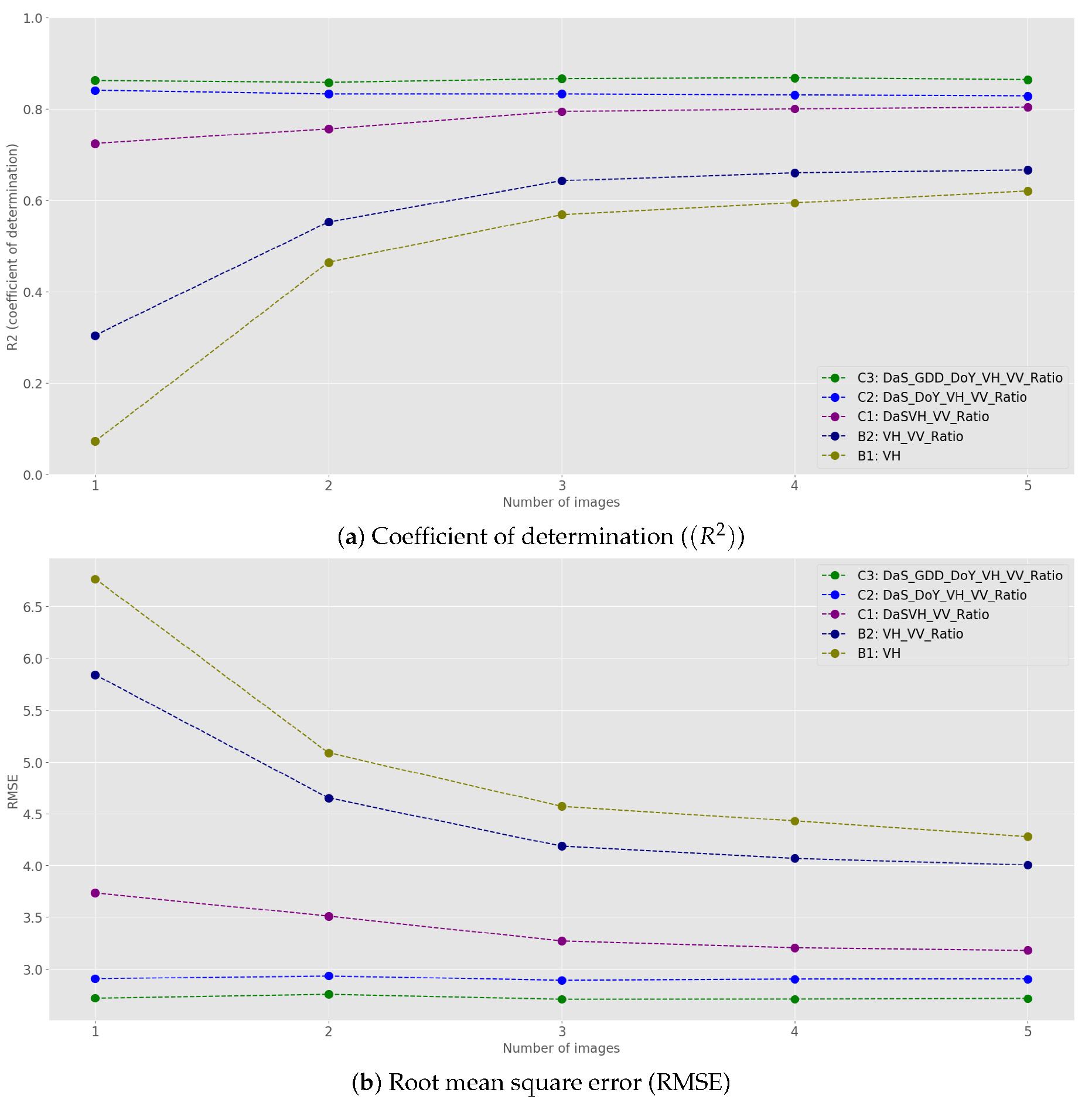
3.2. Multi-Temporal Sar Results
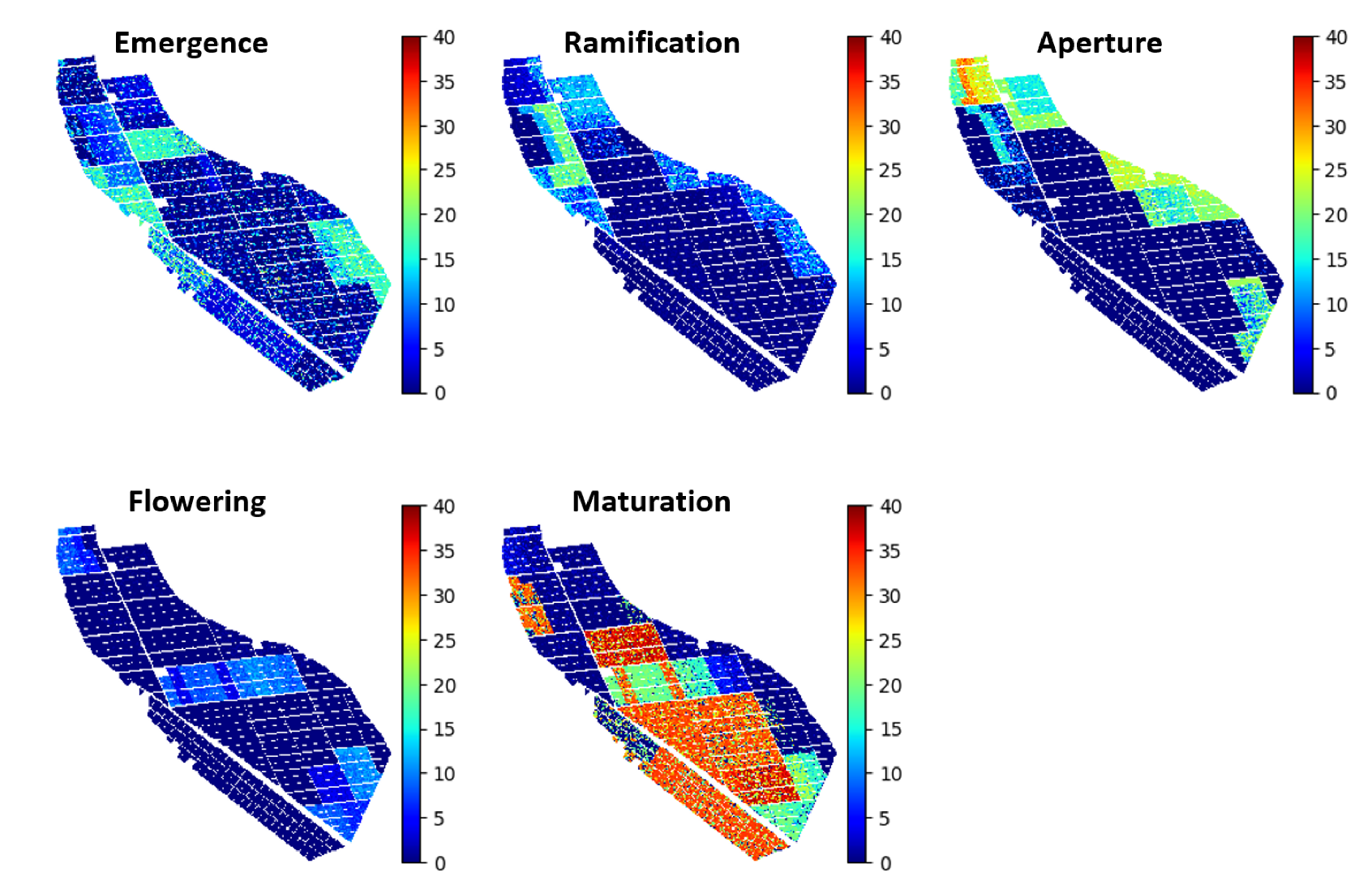
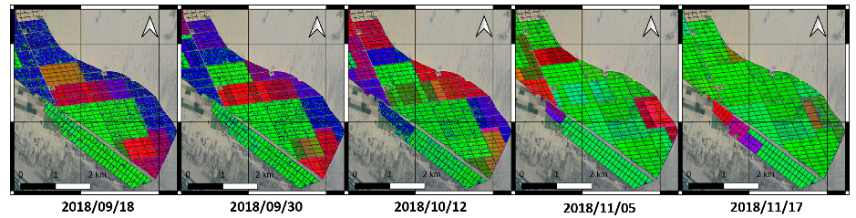
3.3. Growth Stage Estimation Maps
4. Discussion
5. Conclusions
Author Contributions
Funding
Conflicts of Interest
References
- Pedregosa, F.; Varoquaux, G.; Gramfort, A.; AU West, P.C.; Gibbs, H.K.; Monfreda, C.; Wagner, J.; Barford, C.C.; Carpenter, S.R.F.J.A. Trading carbon for food: Global comparison of carbon stocks vs. crop yields on agricultural land. Proc. Natl. Acad. Sci. USA 2010, 107, 19645–19648. [Google Scholar]
- Food and Agriculture Organization of the United Nations. FAOSTAT Crops; FAO: Rome, Italy, 2019. [Google Scholar]
- Terán-Velazco, C.A. Impactos sociales del espárrago en el Perú. 2017. Available online: http://repositorio.ulima.edu.pe/bitstream/handle/ulima/6003/Teran_Esparragos_Peru.pdf?sequence=1&isAllowed=y (accessed on 15 May 2020).
- Hodges, T. Predicting Crop Phenology; CRC Press: Boca Raton, FL, USA, 1990. [Google Scholar]
- Jong-Sen Lee, E.P. Polarimetric Radar Imaging: From Basics to Applications; CRC Press: Boca Raton, FL, USA, 2017. [Google Scholar]
- Lopez-Sanchez, J.M.; Vicente-Guijalba, F.; Ballester-Berman, J.D.; Cloude, S.R. Polarimetric Response of Rice Fields at C-Band: Analysis and Phenology Retrieval. IEEE Trans. Geos. Rem. Sen. 2014, 52, 2977–2993. [Google Scholar] [CrossRef] [Green Version]
- Alonso-Gonzalez, A.; Joerg, H.; Papathanassiou, K.; Hajnsek, I. Change Analysis and Interpretation in Polarimetric Time Series over Agricultural Fields at C-band. In Proceedings of the EUSAR 2016: 11th European Conference on Synthetic Aperture Radar, Hamburg, Germany, 6–9 June 2016; pp. 1–6. [Google Scholar]
- Wiseman, G.; McNairn, H.; Homayouni, S.; Shang, J. RADARSAT-2 Polarimetric SAR Response to Crop Biomass for Agricultural Production Monitoring. IEEE J. Sel. Top. Appl. Earth Obs. Remote Sens. 2014, 7, 4461–4471. [Google Scholar] [CrossRef]
- Veloso, A.; Mermoz, S.; Bouvet, A.; Le Toan, T.; Planells, M.; Dejoux, J.F.; Ceschia, E. Understanding the temporal behavior of crops using Sentinel-1 and Sentinel-2-like data for agricultural applications. Remote Sens. Environ. 2017, 199, 415–426. [Google Scholar] [CrossRef]
- Steele-Dunne, S.C.; Khabbazan, S.; Vermunt, P.C.; Arntz, L.R.; Marinetti, C.; Iannini, L.; Westerdijk, K.; van der Sande, C. Monitoring Key Agricultural CROPS in the Netherlands using Sentinel-1. In Proceedings of the IGARSS 2018—2018 IEEE International Geoscience and Remote Sensing Symposium, Valencia, Spain, 22–27 July 2018; pp. 6639–6642. [Google Scholar] [CrossRef]
- Khabbazan, S.; Vermunt, P.; Steele-Dunne, S.; Ratering Arntz, L.; Marinetti, C.; van der Valk, D.; Iannini, L.; Molijn, R.; Westerdijk, K.; van der Sande, C. Crop Monitoring Using Sentinel-1 Data: A Case Study from The Netherlands. Remote Sens. 2019, 11, 1887. [Google Scholar] [CrossRef] [Green Version]
- Harfenmeister, K.; Spengler, D.; Weltzien, C. Analyzing Temporal and Spatial Characteristics of Crop Parameters Using Sentinel-1 Backscatter Data. Remote Sens. 2019, 11, 1569. [Google Scholar] [CrossRef] [Green Version]
- Küçük, Ç.; Taşkın, G.; Erten, E. Paddy-Rice Phenology Classification Based on Machine-Learning Methods Using Multitemporal Co-Polar X-Band SAR Images. IEEE J. Sel. Top. Appl. Earth Obs. Remote Sens. 2016, 9, 2509–2519. [Google Scholar] [CrossRef]
- Wang, H.; Magagi, R.; Goïta, K.; Trudel, M.; McNairn, H.; Powers, J. Crop phenology retrieval via polarimetric SAR decomposition and Random Forest algorithm. Remote Sens. Environ. 2019, 231, 111234. [Google Scholar] [CrossRef]
- Mascolo, L.; Lopez-Sanchez, J.M.; Vicente-Guijalba, F.; Nunziata, F.; Migliaccio, M.; Mazzarella, G. A Complete Procedure for Crop Phenology Estimation With PolSAR Data Based on the Complex Wishart Classifier. IEEE Trans. Geosci. Remote Sens. 2016, 54, 6505–6515. [Google Scholar] [CrossRef] [Green Version]
- Meier, U. Growth Stages of Mono-And Dicotyledonous Plants; Blackwell Wissenschafts-Verlag: Berlin, Germany, 1997. [Google Scholar]
- Lopez-Sanchez, J.M.; Ballester-Berman, J.D.; Hajnsek, I. First Results of Rice Monitoring Practices in Spain by Means of Time Series of TerraSAR-X Dual-Pol Images. IEEE J. Sel. Top. Appl. Earth Obs. Remote Sens. 2011, 4, 412–422. [Google Scholar] [CrossRef]
- Cota, N.; Kasetkasem, T.; Rakwatin, P.; Chanwimaluang, T.; Kumazawa, I. Rice phenology estimation based on statistical models for time-series SAR data. In Proceedings of the 2015 12th International Conference on Electrical Engineering/Electronics, Computer, Telecommunications and Information Technology (ECTI-CON), Hua Hin, Thailand, 24–27 June 2015; pp. 1–6. [Google Scholar] [CrossRef]
- Siachalou, S.; Mallinis, G.; Tsakiri-Strati, M. A hidden Markov models approach for crop classification: Linking crop phenology to time series of multi-sensor remote sensing data. Remote Sens. 2015, 7, 3633–3650. [Google Scholar] [CrossRef] [Green Version]
- Vicente-Guijalba, F.; Martinez-Marin, T.; Lopez-Sanchez, J.M. Dynamical Approach for Real-Time Monitoring of Agricultural Crops. IEEE Trans. Geosci. Remote Sens. 2015, 53, 3278–3293. [Google Scholar] [CrossRef] [Green Version]
- De Bernardis, C.; Vicente-Guijalba, F.; Martinez-Marin, T.; Lopez-Sanchez, J.M. Contribution to Real-Time Estimation of Crop Phenological States in a Dynamical Framework Based on NDVI Time Series: Data Fusion With SAR and Temperature. IEEE J. Sel. Top. Appl. Earth Obs. Remote Sens. 2016, 9, 3512–3523. [Google Scholar] [CrossRef] [Green Version]
- McNairn, H.; Jiao, X.; Pacheco, A.; Sinha, A.; Tan, W.; Li, Y. Estimating canola phenology using synthetic aperture radar. Remote Sens. Environ. 2018, 219, 196–205. [Google Scholar] [CrossRef]
- Tavakkoli, M.; Lohmann, P.; Soergel, U. Mapping of agricultural activities using Multi-Temporal ASAR ENVISAT DATA. In Proceedings of the ISPRS Hannover Workshop 2007: High-Resolution Earth Imaging for Geospatial Information’, Hannover, Germany, 29 May—1 June 2007. ISPRS Archives—XXXVI-1/W51. [Google Scholar]
- Tavakkoli, M.; Lohmann, P. Multi-temporal classification of ASAR images in agricultural areas. In Proceedings of the ISPRS Commission VII Symposium: ‘Remote Sensing: From Pixels to Processes’, Enschede, The Netherlands, 8–11 June 2006. [Google Scholar]
- Sabour, S.T.; Lohmann, P.; Soergel, U. Monitoring agricultural activities using multi-temporal ASAR ENVISAT data. Int. Arch. Photogramm. Remote Sens. Spat. Inf. Sci. 2008, 37, 735–742. [Google Scholar]
- Bargiel, D.; Herrmann, S.; Lohmann, P.; Sörgel, U. Land use classification with high-resolution satellite radar for estimating the impacts of land use change on the quality of ecosystem services. Int. Arch. Photogramm. Remote Sens. Spat. Inf. Sci. 2010, 38, 68–73. [Google Scholar]
- Arias, M.; Campo-Bescós, M.Á.; Álvarez-Mozos, J. Crop Classification Based on Temporal Signatures of Sentinel-1 Observations over Navarre Province, Spain. Remote Sens. 2020, 12, 278. [Google Scholar] [CrossRef] [Green Version]
- Wien, H.C.; Stützel, H. The Physiology of Vegetable Crops; CABI: Oxfordshire, UK, 2020. [Google Scholar]
- Wilson, D.; Sinton, S.; Butler, R.; Drost, D.; Paschold, P.J.; van Kruistum, G.; Poll, J.; Garcin, C.; Pertierra, R.; Vidal, I.; et al. Carbohydrates and yield physiology of asparagus–A global overview. In XI International Asparagus Symposium 776, Horst, Netherlands; International Society for Horticultural Science (ISHS): Leuven, Belgium, 2005; pp. 413–428. [Google Scholar]
- Wilson, D.; Cloughley, C.; Jamieson, P.; Sinton, S. A model of asparagus growth physiology. In X International Asparagus Symposium 589, Niigata, Japan; International Society for Horticultural Science (ISHS): Leuven, Belgium, 2001; pp. 297–301. [Google Scholar]
- Casas, A. El Cultivo del Espárrago en la Costa Peruana. Available online: http://www.lamolina.edu.pe/agronomia/dhorticultura/html/apuntesdeclase/Casas/El%20Cultivo%20del%20esp%C3%A1rrago%20en%20la%20Costa%20Peruana.pdf (accessed on 15 May 2020).
- Gorelick, N.; Hancher, M.; Dixon, M.; Ilyushchenko, S.; Thau, D.; Moore, R. Google Earth Engine: Planetary-scale geospatial analysis for everyone. Remote Sens. Environ. 2017, 202, 18–27. [Google Scholar] [CrossRef]
- Oh, Y.; Sarabandi, K.; Ulaby, F.T. An empirical model and an inversion technique for radar scattering from bare soil surfaces. IEEE Trans. Geosci. Remote Sens. 1992, 30, 370–381. [Google Scholar] [CrossRef]
- Davidson, M.W.; Le Toan, T.; Mattia, F.; Satalino, G.; Manninen, T.; Borgeaud, M. On the characterization of agricultural soil roughness for radar remote sensing studies. IEEE Trans. Geosci. Remote Sens. 2000, 38, 630–640. [Google Scholar] [CrossRef] [Green Version]
- Yen, Y.f.; Nichols, M.; Woolley, D. Growth of asparagus spears and ferns at high temperatures. In VIII International Asparagus Symposium 415, Palmerston North, New Zealand; International Society for Horticultural Science (ISHS): Leuven, Belgium, 1993; pp. 163–174. [Google Scholar]
- Wilson, D.; Cloughley, C.; Sinton, S. Model of the influence of temperature on the elongation rate of asparagus spears. In IX International Asparagus Symposium 479, Pasco, Washington, USA; International Society for Horticultural Science (ISHS): Leuven, Belgium, 1997; pp. 297–304. [Google Scholar]
- McMaster, G.S.; Wilhelm, W. Growing degree-days: One equation, two interpretations. Agric. For. Meteorol. 1997, 87, 291–300. [Google Scholar] [CrossRef] [Green Version]
- Liang, S. Advances in Land Remote Sensing: System, Modeling, Inversion and Application; Springer Science & Business Media: Berlin/Heidelberg, Germany, 2008. [Google Scholar]
- Oliver, C.; Quegan, S. Understanding Synthetic Aperture Radar Images; SciTech Publishing: Raleigh, NC, USA, 2004. [Google Scholar]
- Caruana, R. Multitask Learning. Mach. Learn. 1997, 28, 41–75. [Google Scholar] [CrossRef]
- Ruder, S. An Overview of Multi-Task Learning in Deep Neural Networks. arXiv 2017, arXiv:1706.05098. [Google Scholar]
- Camps-Valls, G.; Martino, L.; Svendsen, D.H.; Campos-Taberner, M.; Muñoz-Marí, J.; Laparra, V.; Luengo, D.; García-Haro, F.J. Physics-aware Gaussian processes in remote sensing. Appl. Soft Comput. 2018, 68, 69–82. [Google Scholar] [CrossRef]
- Leiva-Murillo, J.M.; Gomez-Chova, L.; Camps-Valls, G. Multitask Remote Sensing Data Classification. IEEE Trans. Geosci. Remote Sens. 2013, 51, 151–161. [Google Scholar] [CrossRef]
- Segal, M.; Xiao, Y. Multivariate random forests. Wiley Interdiscip. Rev. Data Min. Knowl. Discov. 2011, 1, 80–87. [Google Scholar] [CrossRef]
- Breiman, L. Random forests. Mach. Learn. 2001, 45, 5–32. [Google Scholar] [CrossRef] [Green Version]
- Johnson, R.W. An introduction to the bootstrap. Teach. Stat. 2001, 23, 49–54. [Google Scholar] [CrossRef]
- Breiman, L.; Friedman, J.; Stone, C.J.; Olshen, R.A. Classification and Regression Trees; CRC Press: Boca Raton, FL, USA, 1984. [Google Scholar]
- Mahalanobis, P.C. On the Generalized Distance in Statistics; National Institute of Science of India: Brahmapur, India, 1936. [Google Scholar]
- Kim, S.J.; Lee, K.B. Constructing decision trees with multiple response variables. Int. J. Manag. Decis. Mak. 2003, 4, 337–353. [Google Scholar] [CrossRef]
- d’Andrimont, R.; Taymans, M.; Lemoine, G.; Ceglar, A.; Yordanov, M.; van der Velde, M. Detecting flowering phenology in oil seed rape parcels with Sentinel-1 and-2 time series. Remote Sens. Environ. 2020, 239, 111660. [Google Scholar] [CrossRef]
- Skakun, S.; Vermote, E.; Franch, B.; Roger, J.C.; Kussul, N.; Ju, J.; Masek, J. Winter Wheat Yield Assessment from Landsat 8 and Sentinel-2 Data: Incorporating Surface Reflectance, Through Phenological Fitting, into Regression Yield Models. Remote Sens. 2019, 11, 1768. [Google Scholar] [CrossRef] [Green Version]
- Ahmad, L.; Kanth, R.H.; Parvaze, S.; Mahdi, S.S. Growing degree days to forecast crop stages. In Experimental Agrometeorology: A Practical Manual; Springer: Berlin, Germany, 2017; pp. 95–98. [Google Scholar]
- University, M.S. Using Growing Degree Days to Predict Plant Stages. Available online: http://landresources.montana.edu/soilfertility/documents/PDF/pub/GDDPlantStagesMT200103AG.pdf (accessed on 15 May 2020).
- Phan, H.; Le Toan, T.; Bouvet, A.; Nguyen, L.D.; Pham Duy, T.; Zribi, M. Mapping of rice varieties and sowing date using x-band SAR data. Sensors 2018, 18, 316. [Google Scholar] [CrossRef] [PubMed] [Green Version]
- Mascolo, L.; Forino, G.; Nunziata, F.; Pugliano, G.; Migliaccio, M. A New Methodology for Rice Area Monitoring With COSMO-SkyMed HH–VV PingPong Mode SAR Data. IEEE J. Sel. Top. Appl. Earth Obs. Remote Sens. 2019, 12, 1076–1084. [Google Scholar] [CrossRef]
- De Bernardis, C.G.; Vicente-Guijalba, F.; Martinez-Marin, T.; Lopez-Sanchez, J.M. Estimation of key dates and stages in rice crops using dual-polarization SAR time series and a particle filtering approach. IEEE J. Sel. Top. Appl. Earth Obs. Remote Sens. 2014, 8, 1008–1018. [Google Scholar] [CrossRef] [Green Version]
- Tan, B.; Morisette, J.T.; Wolfe, R.E.; Gao, F.; Ederer, G.A.; Nightingale, J.; Pedelty, J.A. Vegetation phenology metrics derived from temporally smoothed and gap-filled MODIS data. In Proceedings of the IGARSS 2008—2008 IEEE International Geoscience and Remote Sensing Symposium, Boston, MA, USA, 7–11 July 2008; IEEE: Piscataway, NJ, USA, 2008; Volume 3, p. 593. [Google Scholar]
- Boschetti, M.; Stroppiana, D.; Brivio, P.; Bocchi, S. Multi-year monitoring of rice crop phenology through time series analysis of MODIS images. Int. J. Remote Sens. 2009, 30, 4643–4662. [Google Scholar] [CrossRef]
- Ozer, H. Sowing date and nitrogen rate effects on growth, yield and yield components of two summer rapeseed cultivars. Eur. J. Agron. 2003, 19, 453–463. [Google Scholar] [CrossRef]


| Pass Direction | Relative Orbit | Inc. Angle | Acquisition Time |
|---|---|---|---|
| Descending | 142 | 35 | 10:54 |
| Ascending | 18 | 31 | 23:34 |
| Ascending | 91 | 45 | 23:42 |
| Category | Scenario | Input | Description |
|---|---|---|---|
| A | A1 | DaS | Only number of days after cultivation started |
| A | A2 | DaS, DoY | Days after cultivation started, Day of year when cultivation started |
| A | A3 | DaS, DoY, AGDD | Days after cultivation started, Day of year when cultivation started, accumulated temperature |
| B | B1 | VH | Only VH polarisation |
| B | B2 | VH, VV, VH/VV | VH, VV polarisations and the VH/VV ratio |
| C | C1 | VH, VV, VH/VV, DaS | VH, VV, Ratio, Days after cultivation started |
| C | C2 | VH, VV, VH/VV, DaS, DoY | VH, VV, Ratio, Days after cultivation started, Day of year when cultivation started |
| C | C3 | VH, VV, VH/VV, DaS, DoY, AGDD | All previous features |
| Hyperparameter | Selected |
|---|---|
| Bootstrap | True |
| The number of trees in the forest | 800 (a) |
| Split funciton | Mahalanobis Distance |
| max-depth | 30 (a) |
| Stage | A1 | A2 | A3 | B1 | B2 | C1 | C2 | C3 |
|---|---|---|---|---|---|---|---|---|
| Emergence | 0.72 | 0.83 | 0.88 | 0.54 | 0.68 | 0.78 | 0.83 | 0.84 |
| Aperture | 0.65 | 0.9 | 0.92 | 0.04 | 0.27 | 0.71 | 0.87 | 0.9 |
| Ramification | 0.74 | 0.9 | 0.9 | −0.22 | 0.11 | 0.81 | 0.9 | 0.9 |
| Flowering | 0.41 | 0.79 | 0.82 | −0.36 | −0.06 | 0.49 | 0.7 | 0.76 |
| Maturation | 0.79 | 0.91 | 0.94 | 0.36 | 0.52 | 0.82 | 0.89 | 0.9 |
| Overall | 0.66 | 0.87 | 0.89 | 0.07 | 0.3 | 0.72 | 0.84 | 0.86 |
| Stage | A1 | A2 | A3 | B1 | B2 | C1 | C2 | C3 |
|---|---|---|---|---|---|---|---|---|
| Emergence | 4.16 | 3.23 | 2.72 | 5.36 | 4.42 | 3.69 | 3.25 | 3.13 |
| Aperture | 3.18 | 1.67 | 1.54 | 5.26 | 4.61 | 2.87 | 1.96 | 1.66 |
| Ramification | 2.2 | 1.34 | 1.34 | 4.78 | 4.09 | 1.87 | 1.36 | 1.35 |
| Flowering | 2.91 | 1.74 | 1.61 | 4.43 | 3.92 | 2.71 | 2.08 | 1.85 |
| Maturation | 6.48 | 4.34 | 3.48 | 11.39 | 9.88 | 6.08 | 4.63 | 4.36 |
| Overall | 4.07 | 2.72 | 2.3 | 6.77 | 5.84 | 3.73 | 2.9 | 2.72 |
| User Case | Season Start Date | Temperature Data | Scenario |
|---|---|---|---|
| Small farm interested in estimating occurrence of key dates for planning | known from ground truth | known from ground station | A * |
| Medium or large size farms | known from ground truth | known from ground station | C2 and C3 ** |
| Large scale monitoring (regional or national level) without temperature | Automatically detected | - | B2 and C2 *** |
| Large scale monitoring (regional or national level) and satellite measurements of land surface temperature | Automatically detected | known from satellite measurements of land surface temperature | C3 **** |
© 2020 by the authors. Licensee MDPI, Basel, Switzerland. This article is an open access article distributed under the terms and conditions of the Creative Commons Attribution (CC BY) license (http://creativecommons.org/licenses/by/4.0/).
Share and Cite
Silva-Perez, C.; Marino, A.; Cameron, I. Monitoring Agricultural Fields Using Sentinel-1 and Temperature Data in Peru: Case Study of Asparagus (Asparagus officinalis L.). Remote Sens. 2020, 12, 1993. https://0-doi-org.brum.beds.ac.uk/10.3390/rs12121993
Silva-Perez C, Marino A, Cameron I. Monitoring Agricultural Fields Using Sentinel-1 and Temperature Data in Peru: Case Study of Asparagus (Asparagus officinalis L.). Remote Sensing. 2020; 12(12):1993. https://0-doi-org.brum.beds.ac.uk/10.3390/rs12121993
Chicago/Turabian StyleSilva-Perez, Cristian, Armando Marino, and Iain Cameron. 2020. "Monitoring Agricultural Fields Using Sentinel-1 and Temperature Data in Peru: Case Study of Asparagus (Asparagus officinalis L.)" Remote Sensing 12, no. 12: 1993. https://0-doi-org.brum.beds.ac.uk/10.3390/rs12121993