Geographic Object-Based Image Analysis: A Primer and Future Directions


Department of Geography, University of Calgary, Calgary, AB T2N 1N4, Canada
*
Author to whom correspondence should be addressed.
Remote Sens. 2020, 12(12), 2012; https://0-doi-org.brum.beds.ac.uk/10.3390/rs12122012
Submission received: 30 April 2020
/
Revised: 19 June 2020
/
Accepted: 21 June 2020
/
Published: 23 June 2020
(This article belongs to the Special Issue GeoAI: Integration of Artificial Intelligence, Machine Learning and Deep Learning with Remote Sensing)
Abstract
:Geographic object-based image analysis (GEOBIA) is a remote sensing image analysis paradigm that defines and examines image-objects: groups of neighboring pixels that represent real-world geographic objects. Recent reviews have examined methodological considerations and highlighted how GEOBIA improves upon the 30+ year pixel-based approach, particularly for H-resolution imagery. However, the literature also exposes an opportunity to improve guidance on the application of GEOBIA for novice practitioners. In this paper, we describe the theoretical foundations of GEOBIA and provide a comprehensive overview of the methodological workflow, including: (i) software-specific approaches (open-source and commercial); (ii) best practices informed by research; and (iii) the current status of methodological research. Building on this foundation, we then review recent research on the convergence of GEOBIA with deep convolutional neural networks, which we suggest is a new form of GEOBIA. Specifically, we discuss general integrative approaches and offer recommendations for future research. Overall, this paper describes the past, present, and anticipated future of GEOBIA in a novice-accessible format, while providing innovation and depth to experienced practitioners.
1. Introduction
Geographic object-based image analysis (GEOBIA) is an image analysis paradigm [1,2] that is typically applied to remote sensing images collected by satellites, piloted aircraft, and drones. GEOBIA is typically used for land-cover/land-use mapping where the image is completely partitioned into classified polygons (i.e., wall-to-wall coverage), as well as for detecting and delineating discrete geographic objects of interest such as individual cars, buildings, and trees [3]. Land-cover/land-use and geographic object mapping with GEOBIA has been demonstrated in agriculture, forestry, urban, and natural hazards remote sensing contexts and more [4]. GEOBIA generally works by organizing an image into image-objects (groups of neighboring pixels that represent real-world geographic objects) and examining those image-objects based on their spectral, textural, geometrical, and contextual features (i.e., attributes) [5]. These features are then used to classify the image-objects, i.e., label them according to the geographic object(s) they represent, which can be a land-cover/land-use class (e.g., urban) or object category (e.g., building, car). The labeled image-objects can then be converted from groups of image pixels to polygons for analysis in a geographic information system (GIS). Thus, GEOBIA is regarded as a bridge between raster-based remote sensing and the vector-based GIS domain [1].
GEOBIA has been an active research field since the early 2000s, with a comprehensive 2014 review paper finding over 600 publications since 2000 [2], while more topic-specific GEOBIA reviews have found lower numbers. These include: (i) a 2017 review paper on land-cover classification, which found 173 publications since 2004 [4]; (ii) a 2018 review paper on land-cover classification accuracy assessment methods, which found 209 publications since 2003 [6]; and (iii) a 2019 review paper on GEOBIA-related image segmentation, which found 290 publications since 1999 [7].
These GEOBIA review papers have: (i) explained why GEOBIA is a recent paradigm [2]; (ii) provided a comprehensive survey and comparison of methodological choices [4]; and (iii) focused on specific methodological aspects [6,7]. However, the literature is missing a current overview of GEOBIA that integrates: (i) theoretical foundations from the seminal literature; (ii) best practices and the status of methodological research; as well as (iii) anticipated future directions within a deep learning context. To address this literature gap, we present an overview of the history and methodology of GEOBIA, followed by a discussion of its recent and evolving integration with convolutional neural networks (CNNs). CNNs are deep learning models that have been applied to remote sensing since 2014 [8,9], and their integration with GEOBIA presents opportunities to improve techniques for segmenting and classifying image-objects using increasingly available H-resolution Earth observation imagery.
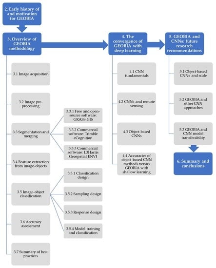
The primary objectives of this paper are to: (i) guide novice practitioners in performing GEOBIA; (ii) describe how the field is evolving with respect to methodological considerations, including integration with CNNs; and (iii) provide recommendations for future research directions. As outlined in Figure 1, the remainder of this paper discusses the early history of and motivation for GEOBIA (Section 2), the methodological workflow (Section 3), the recent convergence of GEOBIA with CNNs (Section 4), and future directions (Section 5). Section 6 provides a summary. Table A1 provides a list of acronyms used in this paper. We note that Section 2 and Section 3 provide background and methodological guidance regarding the conventional framework of GEOBIA, which includes standard approaches that have been developed by 20+ years of research. Because these sections were primarily written for novice practitioners, we intentionally kept this practical guidance separate from the newer, less-standardized integration of GEOBIA with CNNs—Section 4 and Section 5 will discuss this emerging form of GEOBIA.
2. Early History of and Motivation for GEOBIA
The launch of the first Landsat satellite (Landsat-1) in 1972 sparked the beginning of civilian satellite-based remote sensing [5]. The spatial resolution of the sensor onboard Landsat-1 was 80 m [5]. With each pixel sampling 80 m2 of the ground surface, smaller discrete geographic objects such as individual trees and residential roofs were not resolvable, and only general land-cover classes could be observed [5]. Thus, land-cover classification was performed on a pixel-by-pixel basis, where individual pixels were analyzed for their spectral properties, and context was irrelevant [2,10]. Increasingly, however, research conducted after the 1970s showed that image texture [11,12]—which observes the variance and spatial arrangement of neighboring pixels values—could be used to improve spectral-based classification accuracy [2,13]. Earth observation satellites launched throughout the remainder of the century provided medium-resolution (2–20 m) and low-resolution (>20 m) imagery, and pixel-based classification was the standard approach [1]. During this time, finer resolution imagery was generally available only from airborne platforms.
Starting in 1999 with the launch of the IKONOS satellite, high-resolution (<2 m) satellite imagery became commercially available [14]. The availability of such high-resolution satellite imagery (as well as faster computing and more ubiquitous internet access) led to an increase in the ability to produce high-resolution, or H-resolution, remote sensing scene models (see Section 3.1 for details), where individual geographic objects of interest are sampled by many pixels, revealing their geometrical and textural properties [2,15,16,17]. This level of detail is especially beneficial for observing smaller geographic objects such as trees and residential roofs [18]. At the same time, higher-resolution imagery results in higher within-class spectral variability, which could have adverse effects on the accuracy of pixel-based classification [2,12,13,18]. Thus, with the increasing availability of high-resolution imagery, and the release in 2000 of an object-based image analysis (OBIA) commercial software for remote sensing imagery called “eCognition”, OBIA emerged within the geographic information science (GIScience) community [5,14,19].
As OBIA was applied to fields other than remote sensing, including biomedical imaging, astronomy, microscopy, and computer vision, Hay and Castilla [1] established the name GEOBIA (geographic object-based image analysis) to designate the application of OBIA on Earth (i.e., Geo) observation imagery as a GIScience subdiscipline, and provided a number of key tenets that distinguished it from OBIA. Hay and Castilla [1] also listed several reasons why GEOBIA improves upon pixel-based classification: (i) the partitioning of images into image-objects mimics human visual interpretation; (ii) analyzing image-objects provides additional related information (e.g., texture, geometry, and contextual relations); (iii) image-objects can more easily be integrated into a GIS; and (iv) using image-objects as the basic units of analysis helps mitigate the modifiable areal unit problem (MAUP) in remote sensing.
The MAUP refers to a key issue in spatial analysis: that results are dependent on the areal sampling unit [20]. As it relates to remote sensing [21,22], the MAUP describes that different analytical results can be obtained when: (i) observations are made at different scales (i.e., using different spatial resolutions of imagery); and (ii) observations are made using different combinations (i.e., aggregations) of areal units. An example of the latter was provided by Marceau et al. [13], who showed that 90% of the variance in classification accuracy of nine land covers was due to the window size used for texture analysis, and that the optimal window size for each class was different [22]. Hay and Marceau [23] also argued that an object-based framework, as opposed to a pixel-based framework, helps mitigate the MAUP by shifting from arbitrary observation units (pixels) to meaningful observation units (image-objects) that “explicitly correspond to geographical entities” (p. 4).
Another benefit of a geographic object-based approach is that image-object internal characteristics and spatial relationships can be exploited to model classes. Regarding image-object internal characteristics, image segmentation can be performed at multiple levels of scale to capture variably sized image-objects [24,25], which may help with discriminating between classes that are differentiable by size (e.g., cars versus buildings). Regarding image-object spatial relationships, adjacent image-objects corresponding to a low-level class (e.g.,“tree”) may be aggregated to model a high-level class (e.g., “forest”) [21,23,26]. High-level classes can also be complex and composed of several sub-classes. Adjacent image-objects corresponding to these sub-classes may be used to model composite high-level classes such as mixed arable land [10]. Using these approaches, in which high-level classes are explicitly defined by the low-level class(es) they contain, may also help in defining boundaries between high-level classes (e.g., forest and sparse woodland) [2,5]. In all these regards, GEOBIA is a multiscale image analysis framework in which classes are modeled based on image-object internal characteristics and spatial relationships.
3. Overview of GEOBIA Methodology
A wide variety of GEOBIA applications have been demonstrated in the literature. From a review of over 200 case studies from 2004–2016 that used GEOBIA to perform land-cover classification, Ma et al. [4] found that most study areas were classified as urban (29%), forest (24%), agricultural (22%), vegetated (12%), and wetland (4%), with minor categories including landslide, coral reef, flood, benthic habitat/seabed mapping, coal mining areas, and aquatic (9%). They also found that 62% of the studies focused on applications and 38% focused on methodological issues [4]. Therefore, in addition to real-world applications, the research literature has also contributed to advancing GEOBIA methodology. The following sections will provide an overview of the general steps in GEOBIA methodology and related research: (3.1) H-resolution image acquisition; (3.2) image and ancillary data pre-processing; (3.3) classification design; (3.4) segmentation and merging; (3.5) feature extraction and feature space reduction; (3.6) image-object classification; and (3.7) accuracy assessment (Figure 1). Section 3.8 summarizes methodological best practices. This workflow is intended to provide novice users a general series of steps for performing land-cover/land-use mapping with GEOBIA. The workflow may change as the complexity of the application increases. For example, GEOBIA can also be used for time series analysis/change detection (e.g., [27]), geomorphometric/terrain analysis (e.g., [28]), and more.
3.1. H-Resolution Image Acquisition
High-resolution imagery is more commonly used for GEOBIA than lower-resolution imagery [4]; however, GEOBIA can be applied to any H-resolution situation [2]. As noted in Section 2, H-resolution situations occur when the geographic objects of interest are significantly larger (typically 3–5 times) than the pixels they are composed of [2,15,16,17]. Conversely, a low-resolution, or L-resolution, situation occurs when the geographic objects of interest are smaller than the pixels that model them; consequently, individual objects are unresolvable [2,16]. Thus, descriptors such as “high resolution” relate to the spatial resolution of pixels, whereas H-resolution and L-resolution are based on the relationship between the geographic objects of interest and the size of the pixels that model them [5,16]. An H-resolution situation does not necessarily require high-resolution image pixels, as large geographic objects of interest (e.g., forests) can cover an area greater than the pixels of medium- and even low-resolution imagery [2]. To demonstrate that GEOBIA is not constrained to high-resolution imagery (but rather to H-resolution situations [24]), Ma et al. [4] found that, from over 200 case studies that performed land-cover classification with GEOBIA, approximately 50% used 0–2 m spatial resolution imagery, approximately 30% used 2–20 m spatial resolution imagery, and approximately 20% used 20–30 m spatial resolution imagery.
3.2. Image and Ancillary Data Pre-Processing
Once imagery is acquired, appropriate corrections need to be applied, including but not limited to: (i) correcting for atmospheric effects; (ii) orthorectification to correct for image distortion due to the sensor, platform, terrain, and above-ground objects; and (iii) georeferencing to place the image in a desired coordinate system. After image correction, individual image bands can be used to generate new derived images that may be used for image segmentation or classification, such as vegetation index and principal component images [29,30,31,32]. In addition to generating new images, ancillary data can be acquired to aid image segmentation or classification. A common type of ancillary data is raster elevation data in the form of a digital terrain model (DTM) or digital surface model (DSM). A DTM can be subtracted from a DSM to create a normalized DSM (nDSM) with pixel values corresponding to above-ground object heights, which is useful for isolating objects of interest such as buildings and trees [33]. Importantly, Chen et al. [33] noted that all images used in GEOBIA must be co-registered and have the same spatial resolution. For analysis, the aforementioned raster scenes are combined as multiple bands in a single image dataset [33].
3.3. Classification Design
Classification design establishes a legend that provides a simplified model of the image scene with adequate descriptions of each class [2]. Griffith and Hay [31] noted that an object-based classification scheme should be mutually exclusive, exhaustive, and hierarchical. The next step, segmentation and merging (Section 3.4), will produce image-objects that represent geographic objects of different hierarchical levels [5]. Therefore, the legend should contain lower-level classes (e.g., grass, trees, paths, roads, houses) nested within higher-level classes (e.g., urban park). The lower-level classes can be identified during the GEOBIA classification and then aggregated to higher-level classes after the classification (e.g., [29,31]). A pre-defined hierarchical legend introduces organization into the modeling of an image scene [17] and explicitly defines the classes of interest. We note that adding complexity to the classification design will also add complexity to the proceeding steps. For example, if a hierarchical legend is established, the user will need to aggregate lower-level classes to higher-level classes and will also need to decide which level of classes to base the accuracy assessment on. Furthermore, if many similar classes are established in the classification design, then a larger variety of features (attributes) may need to be used in classification.
3.4. Segmentation and Merging
After the image dataset is prepared and the legend is established, a select number of image bands are used for segmentation and merging to partition the scene into multiple components. This combined step is crucial in GEOBIA, where neighboring pixels are grouped together to form image-objects that represent real-world geographic objects [5,17]. There is an important distinction between image segments and image-objects, as explained by Lang [17]: “Segmentation produces image regions, and these regions, once they are considered ‘meaningful’, become image-objects; in other words, an image-object is a ‘peer reviewed’ image region; refereed by a human expert” (p. 13). Several researchers have argued that the accuracy of the segmentation and merging will directly impact the accuracy of the classification, as correctly delineated image-objects will supply spectral, textural, geometrical, and contextual features (i.e., attributes) that are representative of the real-world objects they model [5,30,34]. Castilla and Hay [5] explained that an image-object should be discrete, internally coherent, and should contrast with its neighboring regions. In an ideal segmentation, a one-to-one correspondence exists between image segments and the sought-after image-objects [5], though this is seldom the case in a scene composed of variably sized, shaped, and spatially distributed objects of interest.
Since perfect segmentation of a complex scene is highly unattainable, over-segmentation or under-segmentation are likely [5]. Over-segmentation occurs when the heterogeneity between neighboring segments is too low, thus, too many segments compose the scene, requiring neighboring segments to be merged into single image-objects [5]. Conversely, under-segmentation occurs when the homogeneity of individual segments is too low, thus too few segments compose the scene, and the segments should be segmented into multiple image-objects [5]. From a GEOBIA perspective (in which image-objects are the units of analysis), over-segmentation represents an H-resolution situation, while under-segmentation represents an L-resolution situation. Because a perfect segmentation is highly unlikely, Castilla and Hay [5] recommended that “a good segmentation is one that shows little over-segmentation and no under-segmentation” (p. 96). Over-segmentation is preferred because adjacent segments can be merged [5]. Segment merging can be based on spectral similarity and spatial properties, such as the size of segments [15] or the length of borders between segments [35]. Under-segmentation, on the other hand, has been shown to correspond to segments containing a mixture of objects, which can lead to lower classification accuracies [36,37].
In GEOBIA, image segmentation is typically performed using unsupervised methods [4], though we note that some GEOBIA software such as ENVI Feature Extraction allow user testing and visual feedback of specific segmentation methods in near-real-time (see Section 3.4.3). Unsupervised segmentation algorithms can be categorized as edge-based, region-based, and hybrid [7]. Edge-based segmentation generally works by finding discontinuities in pixel values using edge detection algorithms, and then connecting those discontinuities to form continuous segment edges (i.e., boundaries) [38]. Conversely, region-based methods create segments by growing or splitting groups of pixels using a homogeneity criterion [38]. This criterion can be based on spectral, textural, and/or geometrical properties [38]. It is important to note that, in general, the homogeneity criterion is expressed as a heterogeneity threshold that controls the amount of dissimilarity that is allowed within a segment. While edge-based methods precisely detect segment edges, they tend to experience challenges with creating closed segments [7]. Region-based methods, on the other hand, create closed segments, but often have trouble precisely delineating segment boundaries [7]. Hybrid segmentation methods combine these strengths by detecting segment edges using edge-based methods and growing/merging closed segments using region-based methods [7].
In the GEOBIA literature, the consensus is that determining an optimal segmentation parameter value is a heuristic, subjective, challenging, and time-intensive trial-and-error process [4,6,7,29,30,33,36]. Consequently, in part, research has been conducted to increase objectivity and automation in determining the optimal value, resulting in numerous GEOBIA software options [39]. For example, free and open-source options include (but are not limited to) GRASS GIS [29], Orfeo Toolbox [40], InterIMAGE [41], and RSGISLib [42]. Commercial software options include (but are not limited to) Trimble eCognition [43], L3Harris Geospatial ENVI Feature Extraction [44], Esri ArcGIS Pro [45], and PCI Geomatics Geomatica [46]. The reader is referred to Table (4) in [7] for a description of GEOBIA segmentation approaches available in various free and commercial software, including references to background information.
In their review of over 200 case studies that used GEOBIA for land-cover classification, Ma et al. [4] found that 81% of the studies used Trimble eCognition software (eCognition) [43], while 4% used L3Harris Geospatial ENVI Feature Extraction (ENVI FX) [44]. In the following sections, we will discuss three GEOBIA software options and their associated segmentation and merging approaches: (3.4.1) GRASS GIS; (3.4.2) eCognition; and (3.4.3) ENVI FX. GRASS GIS provides the user with a free and open-source option for performing GEOBIA, while eCognition and ENVI FX are the two most popular commercial options.
3.4.1. Free and Open-Source Software: GRASS GIS
A free and open-source GEOBIA processing chain for GRASS GIS was created by Grippa et al. [29]. The processing chain is semi-automated, Python-coded, and links GRASS GIS modules (tools) with Python and R libraries. The motivation was to provide a free and open-source GEOBIA alternative to black-box commercial software [29]. The image segmentation algorithm in this processing chain uses an unsupervised, bottom-up, iterative region-growing method and is implemented using the GRASS GIS module i.segment [47]. The algorithm requires a user-set threshold parameter (TP). The TP represents a spectral difference threshold, below which adjacent pixels/segments are merged [47]. Specifically, if the similarity distance between adjacent pixels/segments is lower than the TP, then pixels/segments are merged. The TP and spectral similarity distance values are scaled (i.e., they range from 0–1); a TP of 0 will result in identical adjacent pixels/segments being merged, whereas a value of 1 will result in all pixels/segments being merged [47]. The method is iterative—first, adjacent pixels are merged if their similarity distance is: (i) less than the similarity distance between them and their other neighbors, and (ii) less than the TP [47]. Then, adjacent segments are merged if their similarity distance fits the above criteria. This region-growing process continues until no additional merges can be made [47].
The most recent version of the GEOBIA processing chain by Grippa et al. [29] uses a method called spatially partitioned unsupervised segmentation parameter optimization (SPUSPO) to calculate the TP for different spatial subsets of the input data [30]. SPUSPO is a local TP optimization approach based on the concept of spatial non-stationarity, i.e., that the optimal TP varies spatially, especially in heterogeneous scenes like urban areas [30]. Therefore, instead of calculating a single, global TP based on the spatial extent of the input data, a local TP is calculated for each spatial subset of the data using the following procedure, as described by Georganos et al. [30]. SPUSPO first generates spatial subsets by using a computer vision technique called cutline partitioning, which avoids creating subset boundaries through objects like roofs, and instead detects edges and creates boundaries along linear features like streets and roof edges. Cutline partitioning is implemented using the GRASS GIS module i.cutlines [48], though we note that users also have the freedom to adjust the processing chain to use methods other than cutline partitioning to create spatial subset boundaries [30].
Once subsets are created, the optimal TP is calculated for each subset through the following steps, which are implemented using the GRASS GIS module i.segment.uspo [49]. First, a range of TP values is established: the user heuristically determines the minimum and maximum values that result in over- and under-segmentation, respectively. The user also specifies a step value which will determine how many TP values within the range are evaluated. The quality of each segmentation is evaluated by calculating Moran’s I (MI) and weighted variance (WV) values. Moran’s I quantifies the degree of spatial autocorrelation, i.e., how spectrally similar neighboring segments are. The lower the MI value, the higher the inter-segment heterogeneity, which is desired. Weighted variance quantifies the spectral variance within each segment, weights it by the segment’s area, and averages all the values to produce a mean within-segment spectral variance. The lower the WV value, the higher the intra-segment homogeneity, which is desired. The MI and WV for each segmentation are used to calculate an F-score, which quantifies the degree of harmony between inter-segment heterogeneity (MI) and intra-segment homogeneity (WV). The F-score ranges from 0–1; the TP value of the segmentation with the highest F-score is chosen as the optimal TP. In summary, the optimal TP is calculated for each spatial subset, and then image segmentation is performed on each subset. Georganos et al. [30] compared the thematic and segmentation accuracies acquired using SPUSPO and a global unsupervised segmentation parameter optimization. SPUSPO (the local approach) resulted in significantly higher thematic accuracies and less over-segmentation than the global approach [30].
3.4.2. Commercial Software: Trimble eCognition
The most commonly used segmentation algorithm in the research literature is Trimble eCognition’s multiresolution segmentation (MRS) [7,50], which, like the segmentation algorithm used by GRASS GIS SPUSPO, is an unsupervised, bottom-up, iterative region-growing method that requires a user-set scale parameter (similar to the TP in GRASS GIS SPUSPO). MRS performs region-growing segmentation using the following general procedure, as outlined by Trimble [51]. Starting at the pixel level, adjacent pixels are merged if they are homogeneous. The process loops by merging consecutively larger groups of pixels until no further merges can be made. The unitless user-set scale parameter represents the heterogeneity threshold, below which merging occurs, and above which merging stops. The higher the scale parameter, the higher the allowed within-segment heterogeneity, and thus the larger the resulting image segments. For a given scale parameter, heterogeneous regions will have smaller segments than homogeneous regions. The scale parameter is defined as the maximum standard deviation of the homogeneity criteria, which are a weighted combination of color and shape values. The user can adjust the relative weights (importance) assigned to each. Of the user-set parameters in MRS, the scale parameter is regarded as the most important [4,29,30,36]. The scale parameter is also the most challenging to set, as it is unitless and not visually related to the physical structure in the scene [21].
Similar to GRASS GIS SPUSPO, eCognition allows for a statistical optimization of the scale parameter through the popular plug-in software tool Estimation of Scale Parameter 2 (ESP2) [25]. ESP2 uses local variance (LV) to determine an optimal segmentation scale parameter, similar to how Woodcock and Strahler [18] used LV to determine an optimal scale of observation (i.e., spatial resolution) for a given remote sensing scene. Specifically, Woodcock and Strahler [18] applied a 3 × 3 pixel moving window to an image to calculate the standard deviation of the pixel values, and then averaged the standard deviations to obtain an LV for the entire image. They repeated this process with several down-sampled (i.e., coarsened) versions of the image, and graphed LV as a function of spatial resolution. From the graph, they found that the spatial resolution that corresponded to the peak LV, which they deemed the optimal image resolution, tended to approximate the sizes of objects in the scene [18]. They conducted this process for different scene types: forest, urban/suburban, and agricultural. With each scene composed of different-sized objects, Woodcock and Strahler [18] showed that the optimal scale of observation (spatial resolution) was a function of the size of the objects in the scene, and that a graph of LV could be used to describe this relationship. Hay et al. [24] built on this this idea and incorporated it, not globally for an entire scene, but instead for the individual tree objects composing a scene, from which optimal spatial, spectral, and variance measures were defined for each object.
Using the LV concept, the ESP2 tool in eCognition finds the optimal scale parameter using the following general procedure [25,52]. First, the image is segmented using a low segmentation scale (i.e., low scale parameter) in the MRS algorithm. Then, ESP2 calculates the LV of the segmented image, which is the mean within-segment standard deviation. It does this for progressively higher levels of segmentation (i.e., higher values of the scale parameter). Then, it graphs the LV and the rate of change in LV as functions of the scale parameter and uses these graphs to find the optimal scale parameter. The general concept is that, starting from a small scale parameter, as the scale parameter increases, so does the within-segment heterogeneity (LV). Once the segment boundaries surpass individual image-objects and begin to capture the background signal, the LV levels off, similar to the sill in semivariogram analysis [12]. Thus, the optimal scale parameter is associated with the peak in LV before the stagnation [52]. The ESP2 tool can be used on multiple image layers simultaneously and provides an optimal scale parameter for three levels of hierarchy to capture image-objects of different sizes [25].
The GRASS GIS and eCognition segmentation techniques are both multiscale and optimizable but use a different approach. The GRASS GIS technique (SPUSPO) first partitions the image and then determines an optimal local parameter value for each spatial subset, while the eCognition optimization technique (ESP2) determines an optimal global parameter value for three levels of scale. Another difference between the methods is that SPUSPO equally considers measures of intra-segment homogeneity and inter-segment heterogeneity to evaluate segmentation quality, whereas ESP2 only uses intra-segment homogeneity (i.e., LV, with lower values indicating higher homogeneity). Hossain and Chen [7] advised that a segmentation method should equally consider intra-segment homogeneity and inter-segment heterogeneity. Nevertheless, there is a research gap regarding how these segmentation optimization methods compare. We encourage future research to compare these two approaches.
Furthermore, it is challenging for a single local or global parameter value to represent the varying heterogeneity of many different image-objects composing a complex scene. Thus, future approaches that optimize segmentation based on individual image-objects (as described by Hay et al. [24]) rather than on broader scales may improve upon the GRASS GIS and eCognition techniques. This is especially relevant, as these two parameter selection methods are based on somewhat arbitrary scene subsets and levels of scale and are thus likely to be overly biased by the MAUP. We note that a recent approach by Zhang et al. [53] also focused on determining the optimal parameter value for each image-object in the scene. We suggest that in future studies, such object-scale approaches should be compared to the GRASS GIS and eCognition local- and global-scale approaches.
3.4.3. Commercial Software: L3Harris Geospatial ENVI FX
ENVI FX is the second most popular commercial software for performing land-cover classification with GEOBIA [4]. ENVI FX uses a hybrid segmentation method consisting of a watershed transformation followed by segment merging that combines aspects of edge-based and region-growing methods [32,35,38,54]. Segmentation is performed using the following general procedure, as described by L3Harris Geospatial [32,35,54]. The watershed transformation uses the concept of a hydrologic watershed, where water fills each catchment basin starting at the lowest elevations and stops at the highest elevations where adjacent basins meet. With this technique, images are analogous to watersheds, where the lowest pixel values correspond to the bottoms of basins, and the highest pixel values correspond to basin boundaries. The watershed transformation “floods each basin” starting with the lowest pixel values, which grows regions until adjacent regions meet at the pixels with the highest values. The image used for this process can be a gradient image, which is computed using Sobel edge detection, or an intensity image, which is computed by averaging the bands of select input images. The user-set parameter controlling the watershed transformation is the scale level, which is defined as the percentage of the normalized cumulative distribution of the pixel values in the gradient or intensity image. For example, a scale level of 20 indicates that the “flooding” of the “basins” would start from the lowest 20 percent of the pixel values, which controls the minimum size of initial regions. After the watershed transformation, adjacent segments are merged based on their spectral similarity and the length of their common boundary.
From the authors’ experience, ENVI FX offers an intuitive visual interface where the user can easily adjust segmentation parameters using slider bars and view the resulting image segmentation in near-real-time. This visual framework significantly eases the challenging process of manual segmentation parameter tuning and provides a vision-based optimization alternative to the statistical techniques in GRASS GIS SPUSPO and eCognition ESP2. Figure 2, Figure 3 and Figure 4 show segmentation performed on the same image using three software tools: GRASS GIS SPUSPO, eCognition ESP2, and ENVI FX. Figure 2 shows the true-color remote sensing subset image used for the demonstration. The image has a 0.3 m spatial resolution and was acquired in 2014 over Los Angeles County, California, USA, with a Leica ADS81 airborne imaging sensor (red, green, blue, and near-infrared bands) [55].
Segmentation can be performed using a dialog box in eCognition ESP2 and ENVI FX (the reader is referred to Figure A1 for an image of each dialog box). At the time of writing, GRASS GIS SPUSPO did not have a dialog box because the GRASS GIS GEOBIA processing chain consists of Python-based scripts that link multiple GRASS GIS modules with Python and R libraries. We note that for users without programming experience, this processing chain may be more difficult to implement. Figure 3 shows the segmentation preview that is available in ENVI FX. When the user adjusts the slider bars in the ENVI FX dialog box, the segmentation preview updates in near-real-time (Figure 3).
Figure 4 shows the segmentation result for GRASS GIS SPUSPO, eCognition ESP2, and ENVI FX. In each of these images, the primary objective was to accurately segment the rooftops, roads, trees, then grass yards, in this order. Due to the varying size, shape, and spatial distribution of these different image-object classes, some of the classes were segmented more accurately than others, which exemplifies the need for a multiscale approach over an approach that segments variably sized objects within the scene using the same parameters. Based on our experience implementing the different requirements for each software assessed, the fastest and most user-friendly method to implement was ENVI FX, followed by eCognition ESP2, and finally GRASS GIS SPUSPO.
3.5. Feature Extraction and Feature Space Reduction
Once image segmentation and merging are complete, features are extracted from each image-object. We note that these “features” are referred to as “attributes” in the GIS domain. Features can be spectral, textural, geometrical (spatial), or contextual, and can be calculated from a variety of images (e.g., spectral, texture, elevation, principal component, vegetation index) [33]. Table 1 provides examples of features for each category.
These features are used to train a classification model, where each feature serves as an explanatory variable. All the features can be used to build the model, or a subset of the most influential features can be identified and used (this is called feature space reduction) [33]. Feature space reduction typically uses training data and algorithms to identify the most relevant features for classifying the image-objects in the scene [33]. As many features tend to be correlated, reducing the number of features will reduce model complexity/redundancy and computational demand [4,33,37]. Furthermore, some studies have found that there is no significant difference in classification accuracy when using all the features versus using feature space reduction [31,37]. For example, Griffith and Hay [31] showed no significant difference in overall accuracy when using a comprehensive set of 86 spectral, texture, and spatial features versus a reduced set of 9 spectral features. Another advantage of feature space reduction is that the user gains a better understanding of which features are most influential in discriminating between classes [36].
Machine-learning feature space reduction methods are advantageous because they do not assume a specific data distribution [33]. Ma et al. [60] systematically evaluated the effect of different feature space reduction methods on classification accuracy. They performed GEOBIA on drone imagery from an agricultural study area and compared the overall accuracy achieved with a random forest (RF) classifier and support vector machine (SVM) classifier, with and without feature space reduction [60]. They evaluated feature importance evaluation methods, which provide a ranking of influential features, as well as feature subset evaluation methods, which provide a subset of the most influential features. They found that feature importance evaluation methods achieved significantly higher overall accuracies compared to no feature space reduction, whereas feature subset evaluation methods did not significantly improve overall accuracy [60]. They also found that SVM benefits more than RF from feature space reduction, especially with small training sample sizes, and that RF is more robust regarding the number of features used for classification [60]. They generally recommended the use of 15–25 input features for the RF classifier, and 10–20 input features for the SVM classifier [60]. Chen et al. [33] noted that there is no consensus in the GEOBIA community as to which feature space reduction method is superior; however, the ideal method will perform accurately and efficiently, and will be easy to use and available in commercial or free and open-source software.
In eCognition, the feature space optimization (FSO) tool can be used for feature space reduction via a feature subset evaluation method [51]. This tool uses nearest neighbor (NN) classification to determine which combination of features results in the highest mean minimum separation distance between samples of different classes [51]. From a review of over 200 case studies that used GEOBIA for land-cover classification, Ma et al. [4] found that only 22% of studies performed feature space reduction, and that the FSO tool in eCognition was among the most popular methods used. In ENVI FX, feature space reduction can be performed using a feature importance evaluation method called interval-based attribute ranking [61,62]. Generally, this method considers the range of values that correspond to each feature-class combination. For a given feature, the less these ranges overlap among all the classes (which indicates higher class separability), then the higher the discriminating capability index (i.e., importance score) that is assigned to the feature. The features are then ranked based on their importance scores [62]. In the GRASS GIS GEOBIA processing chain [30], feature space reduction can be performed using a hybrid method called variable selection with random forests (VSURF) that is implemented using the R package VSURF [63,64]. This method uses RF classification to first calculate the importance score for each feature based on out-of-bag error. The n features with the highest importance scores are retained. The retained features are then used to construct different subsets, of which one is chosen based on out-of-bag error [63].
We note that feature space reduction capabilities may be imbedded within a classifier. For example, several algorithmic implementations of the RF classifier can calculate importance scores [63], and eCognition’s FSO tool uses NN classification. These tools can be used for feature space reduction purposes only, where the most important features are identified, or they can also be used for classification using the identified features. We refer the reader to Section 3.6.3 (model training and classification) for classifier recommendations.
3.6. Image-Object Classification
Following feature extraction and optional feature space reduction, a classification model is typically trained to classify the image-objects. This supervised classification consists of multiple steps, which will be discussed in the following sections: (3.6.1) sampling design (i.e., generating training and testing sample locations); (3.6.2) response design (i.e., labeling the training and testing samples); and (3.6.3) classification (i.e., training a model and classifying image-objects). The sampling design and response design also impact the accuracy assessment, which will be discussed in Section 3.7.
3.6.1. Sampling Design
Sampling design is used to determine: (i) the minimum per-class sample size; (ii) the sampling units for the test samples (i.e., pixels or polygons); and (iii) how training and test sample locations are selected [6]. In terms of training samples (i.e., the image-objects that will be used to train the classification model), generally, as the number of high-quality training samples increases, overall accuracy increases [65,66]. Perlich and Simonoff [67] demonstrated how to use learning curves to assess the effect of training set size on overall accuracy. Learning curves show generalization performance (represented by overall accuracy or similar metrics) as a function of training set size. For example, if the learning curve shows a continual increase in accuracy, this suggests that collecting more training samples would improve accuracy. If the curve begins leveling off, then the point at which this occurs is an indicator of sufficient sample size [65,67]. The ideal dataset will have class balance—that is, an equal number of samples per class [68]. Class imbalance can cause the less common classes to be underpredicted and the more common classes to be overpredicted by the model [65,69]. We also note that the quality of the training data will impact classification accuracy [65]. The training samples should be accurately labeled and should fully represent the classes being mapped [69].
For test samples (i.e., the samples that will be used to quantify the accuracy of the classification), Ye et al. [6] suggested a minimum of 50 samples per class, though it is unclear whether this number refers to pixel or polygon units. From a review of 181 articles that performed sampling strategies in GEOBIA, they found that 66 articles (36%) collected more than 50 samples per class, 43 articles (24%) collected less than 50 samples per class, and 72 articles (40%) did not report per-class sample size [6]. In terms of test sampling units, from a review of 209 GEOBIA articles, Ye et al. [6] found that 93 articles (45%) used polygon sampling units, while 107 articles (51%) used pixel sampling units, and 9 articles (4%) used both. They also found that articles from 2014–2017 most commonly used polygon sampling units, suggesting that this is becoming the standard approach [6]. We note that the ideal test set will contain as many high-quality samples as possible (and necessary), with an equal number of samples per class [68].
Sample locations are generated with probabilistic methods such as simple random, stratified random, and systematic sampling [6]. For simple random and stratified random sampling, researchers warn against generating random points on the image to randomly select image-objects, as this approach would favor larger image-objects, violating the assumption that each image-object has an equal probability of being selected [3,6,70]. Instead, the recommended alternative is called the list-frame approach: this includes generating a list of the image-objects, randomly shuffling the list, and selecting the first n image-objects as the samples [3,6,70]. For simple random sampling, this is done once for all the image-objects. Griffith and Hay [31] used this type of sampling approach to avoid introducing sampling bias due to image-object size. For stratified random sampling, a separate list of image-objects is generated for each stratum (class), and each list is shuffled and then selected from. The stratified random sampling approach can ensure an equal number of samples per class; however, it requires a fully labeled reference map to allow for the stratification. To achieve class balance without generating a fully labeled reference map, we recommend using the list-frame approach in conjunction with a random sampling strategy using the following steps: (i) generate a randomly shuffled list of all the image-objects; (ii) starting from the first image-object on the list, label each image-object according to the response design (as explained in the next section), while keeping track of the number of samples per class; (iii) once a class has the desired number of samples, skip labeling all subsequent image-objects pertaining to that class; (iv) continue labeling image-objects on the list until all classes have the desired number of samples. We note that class imbalance may be unavoidable when a class occupies a small proportion of the image and is not represented by enough image-objects. In this case, it is especially important to observe per-class accuracies, as overall accuracy will be less affected by misclassifications in rare classes than by misclassifications in more common classes [69,70]. We refer the reader to Section 3.7 for more information on per-class accuracies. We also note that this suggested sampling approach is not explicitly programmed into the three software options that were previously discussed, so the user will need to implement the approach either within or outside of the GEOBIA software.
3.6.2. Response Design
The training and testing image-objects that are randomly selected using the list-frame approach need to be labeled according to the classification design (i.e., legend) and response design. Reference data can be collected in the field from pre-existing thematic maps or GIS data, or from the interpretation of H-resolution remotely sensed images [6]. Chen et al. [33] and Stehman and Foody [70] noted that drone imagery is a good candidate for augmenting or replacing field-based reference data from the standpoint of time and cost efficiency, though we note that this will depend on the size of the study area. From a review of 209 publications that performed GEOBIA, Ye et al. [6] found that most studies interpreted satellite imagery to obtain reference data, though Whiteside et al. [71] stressed the importance of reducing the temporal lag between the classification and reference data. Similarly, Stehman and Foody [70] noted that the imagery used for classification may also be used as reference data, as long as there is a rigorous protocol for visually interpreting the imagery and determining ground-truth labels.
The image-objects selected as training and test samples can be labeled by superimposing them on (geometrically corrected) reference field data, maps, or remotely sensed imagery. As explained in Section 3.4, image-objects composed of mixed objects have been shown to correspond to lower classification accuracies [36,37]; additionally, the goal is to have no under-segmentation and little over-segmentation [5]. However, when image-objects composed of mixed objects occur, the class label can be assigned based on the class encompassing the most area [4,31].
3.6.3. Model Training and Classification
Various methods exist for performing classification in GEOBIA, including rule-based approaches, where classifications are made based on predefined rulesets [72]. These rulesets may be constructed by domain experts (i.e., expert-based or expert system classification [73,74]). Another approach is supervised classification, where a classification algorithm is trained using examples [72]. According to Ma et al. [4], supervised classification has become the dominant approach since 2010 for land-cover classification using GEOBIA.
In supervised classification, the labeled training image-objects and their corresponding features (i.e., attributes) are used to train a classification model. Increasingly, popular classifiers are machine learning algorithms. From a review of over 200 case studies that used GEOBIA for land-cover classification, Ma et al. [4] found that 29% of the studies used NN, 25% used SVM, 20% used RF, 15% used decision tree (DT), 6% used maximum likelihood classification (MLC), and 5% used other classifiers. Studies that used the RF classifier reported the highest mean overall accuracy, followed in descending order by SVM, DT, NN, and MLC [4].
Similarly, Li et al. [37] performed GEOBIA with drone imagery at an agricultural study area and compared the overall accuracies obtained with k-nearest neighbors (KNN), RF, DT, AdaBoost, and SVM. They found that (i) RF provided the highest accuracies, (ii) KNN provided the lowest accuracies, (iii) RF and DT provided the most stable accuracies with and without feature space reduction, and (iv) RF and SVM were most robust regarding over-segmentation. Overall, Li et al. [37] recommended RF for performing GEOBIA in agricultural study areas.
Whereas RF is generally robust regarding user-set parameter settings and feature space dimensionality [65,69], we reiterate that SVM has shown to be highly accurate when training sample sizes are small [75]. For explanation and guidance regarding RF and SVM, the reader is referred to [66,68,69,75,76,77,78,79]. RF- and SVM-based classification are available in the GRASS GIS GEOBIA processing chain [29] and eCognition [51], while SVM is available in ENVI FX [61].
3.7. Accuracy Assessment
A GEOBIA accuracy assessment, in which thematic (and sometimes geometric) accuracy is assessed, is composed of the sampling design, the response design, and a comparison of the classified image-objects to the labeled test samples [6]. The sampling design and response design, which play a role in the generation of test samples, have already been discussed in Section 3.6. To determine thematic accuracies, the reference class and GEOBIA class of test samples are compared. Ye et al. [6] found that, out of 209 studies, 72% used a confusion matrix, from which standard thematic accuracy statistics were derived, including per-class user’s and producer’s accuracies, overall accuracy, and the Kappa coefficient. We note that the Kappa coefficient, which is an accuracy measure that is corrected for chance agreement, is often reported, but there is a growing argument against its use in the remote sensing domain [70]. Pontius Jr. and Millones [80] explained that the Kappa coefficient can be misleading and flawed for practical applications in remote sensing. Furthermore, overall accuracy and the Kappa coefficient have been shown to be highly correlated [81]; researchers argue that reporting the Kappa coefficient is redundant and rarely contributes new insight [70,80]. Therefore, we recommend using the confusion matrix to calculate and report overall accuracy and per-class user’s and producer’s accuracies. As previously noted, observing per-class accuracies is especially important when class balance cannot be achieved [69,70]. Examining class accuracies using a confusion matrix can also be very useful for further refining training and test samples, which can ultimately improve classification accuracy. For example, using a confusion matrix, Griffith and Hay [31] found that there was confusion between different vegetation classes, between concrete and other bright impervious surfaces, and between non-rooftop impervious surfaces and vegetation. The GRASS GIS GEOBIA processing chain, eCognition, and ENVI are capable of producing confusion matrices [29,82,83].
Another approach for GEOBIA accuracy assessment is to produce an independent digitized reference layer and to label all the image-objects. Ye et al. [6] recommended this approach, as the previously described approach assumes that GEOBIA-generated image-objects correctly represent the landscape. Furthermore, an approach that uses reference geometry could be used to assess GEOBIA segmentation accuracy. We suggest caution with the use of manually digitized reference polygons, as they are subject to human error. To assess thematic and segmentation accuracy using a digitized reference layer, studies overlay the reference layer and GEOBIA-classified layer, and use a pre-defined overlap requirement (e.g., > 50%) to match reference polygons to their corresponding GEOBIA polygons [6]. While useful, Ye et al. [6] reported they were unable to determine a standard approach for matching reference polygons with GEOBIA polygons. Nevertheless, once polygons are matched, their classes can be compared to derive thematic accuracies using a confusion matrix. Their geometries can also be compared to assess segmentation accuracy. Segmentation accuracy evaluation methods used in the literature include area-based measures to calculate under- and over-segmentation, position-based measures to calculate location accuracy, and shape-based measures [3,6,71,84]. Out of 209 reviewed studies, Ye et al. [6] found that only 34 studies (16%) performed segmentation accuracy assessment. However, 30 of the 34 studies were published since 2010, suggesting that evaluating segmentation accuracy is becoming more popular in GEOBIA [6]. Nevertheless, among the 34 studies, there were 11 different methods to assess segmentation accuracy, indicating this aspect of GEOBIA accuracy assessment needs more standardization [6].
3.8. Summary of Best Practices
Section 3.1, Section 3.2, Section 3.3, Section 3.4, Section 3.5, Section 3.6 and Section 3.7 provided details on the general steps involved in GEOBIA methodology, including: (3.1) H-resolution image acquisition; (3.2) image and ancillary data pre-processing; (3.3) classification design; (3.4) segmentation and merging; (3.5) feature extraction and feature space reduction; (3.6) image-object classification; and (3.7) accuracy assessment. To assist users, Table 2 summarizes key requirements and recommendations related to each of these steps.
4. The Convergence of GEOBIA with Convolutional Neural Networks
The conventional GEOBIA framework, which was described in Section 2 and Section 3, has been an active research area in GIScience for the past two decades. As was discussed in Section 3, there is ongoing research regarding many methodological components of conventional GEOBIA, such as image segmentation, feature space reduction, classification, and accuracy assessment. In this section, we introduce the use of convolutional neural networks (CNNs) with remote sensing imagery and describe how their integration with GEOBIA is emerging as a new form of GEOBIA: geographic object-based convolutional neural networks.
CNNs are one of many forms of deep learning that are applied to remote sensing. Deep learning is a subset of machine learning algorithms that uses artificial neural networks composed of many layers [85]. Artificial neural networks are loosely conceptually modeled after biological neural networks [85], and CNNs (one type of artificial neural network) were particularly inspired by the animal visual cortex [85,86,87]. CNNs perform image segmentation, feature extraction, and classification, though in a different manner than GEOBIA. Other deep learning models applied to remote sensing include autoencoders, recurrent neural networks, deep belief networks, and generative adversarial networks. For more information on these topics, we refer the reader to review papers [8,9,88,89,90,91]. In this discussion, we focus on CNNs, as they are the most commonly used deep learning model for remote sensing image analysis [9,90,91]. To better understand this motivation and its evolution, we provide a brief overview of CNNs (Section 4.1), followed by a discussion of their use in remote sensing (Section 4.2 and Section 4.3). Then, we describe general geographic object-based CNN (GEOCNN) approaches that integrate the segmentation, feature extraction, and classification capabilities of GEOBIA and CNNs (Section 4.4). Finally, we present the accuracies of GEOCNN methods versus conventional GEOBIA (Section 4.5). Throughout Section 4, we use the term “GEOBIA” to refer to the conventional framework that was described in the previous sections.
4.1. CNN Fundamentals
Whereas substantial gains in GEOBIA research have been made in the last two decades in the form of hundreds of publications, a related remote sensing subfield has emerged in the last six years: the application of CNNs [8,9]. Essentially, a CNN is a deep learning technique that was designed to work with arrays of data such as one-dimensional signals or sequences and two-dimensional visible-light images or audio spectrograms [86]. Since images are composed of one or more two-dimensional arrays of data (i.e., raster bands), CNNs are conducive to image analysis tasks and are the most common type of deep neural network applied to images [85,86] due to their high generalization capabilities, which stem from the features they extract and their ability to train on extremely large datasets (i.e., thousands or millions of samples) [86,92]—see Section 5.3 for details.
A CNN takes imagery as input, extracts features from it, and uses these features for classification in various manners, depending on the type of CNN. While an in-depth conceptual overview of CNNs is beyond the scope of this paper, we refer the reader to the novice-accessible primers by Yamashita et al. [87] and Chartrand et al. [85], part of which we summarize as follows. Generally, CNNs (like all artificial neural networks) are composed of a series of layers, with each layer containing neurons (i.e., nodes) that perform mathematical operations [85,87]. Neurons within the same layer are not connected; rather, neurons of different layers are connected. The first layers of a CNN correspond to feature extraction: these are called convolutional and pooling layers. Each convolutional layer performs convolution operations using different kernels (i.e., small two-dimensional arrays of numbers) to produce feature maps, which show the locations within the image of each feature. Pooling layers down-sample (i.e., smooth or generalize) the feature maps before passing them to the next convolutional layer. After the convolutional and pooling layers extract features, there are other layers that use these features to perform classification: these are called fully connected layers. The last fully connected layer provides a prediction pertaining to the class of a sample. CNN architectures typically start with multiple “stacks”, each containing several convolutional layers and a pooling layer, followed by fully connected layers [87]. Generally, an artificial neural network is considered “deep” if it contains more than one intermediate fully connected layer (i.e., hidden layer) [9,85,93,94].
4.2. CNNs and Remote Sensing
CNNs have been increasingly applied in the remote sensing literature since 2014 [8,9]. Though promising, the application of CNNs to remote sensing image classification is relatively new, and there are requirements that challenge their ease of use: (i) they have numerous hyperparameters that must be specified by the user; (ii) they require large training samples sizes (i.e., thousands) to combat overfitting; (iii) their training times are long compared to “shallow” machine learning classifiers (such as RF and SVM); and (iv) they have greater complexity than shallow classifiers, thus they are more prone to being used as “black boxes”.
GEOBIA and CNNs are similar in that they both extract features (i.e., attributes) from imagery and then use those features to train a classifier. They differ in terms of how they extract features, and how the features are used for classification. Whereas GEOBIA extracts human-engineered features from image-objects (i.e., texture, spectral, geometrical, and contextual attributes), CNNs extract hierarchical, data-defined features from input imagery, typically using square kernels. The CNN feature hierarchy is not pre-defined or guided by humans but instead is data-driven [86]. As a simplified example in an urban remote sensing context, the first convolutional layer may extract low-level, generic features such as straight lines, curved lines, corners, and “blobs” (binary large objects, i.e., neighboring pixels with similar digital numbers [95]). The line and corner features may correspond to roof or roof-object edges, while blobs may correspond to homogeneous portions of roofs. The next convolutional layer may combine certain low-level features to extract mid-level features such as roof objects (e.g., chimneys, solar panels) or vegetation over roofs. The last convolutional layer may combine mid-level features to extract high-level features, e.g., entire rooftops. With an adequate number of feature-extraction layers, CNN-derived hierarchical features can be robust with respect to changes in translation, scaling, and rotation [92], and have been reported to have better generalizability on unseen test data than human-engineered features [96,97]. For GEOBIA, a shallow machine learning classifier like SVM or RF uses an entire set of human-engineered features, or a subset of the most important features. CNNs, on the other hand, automatically extract features based on the data and learn which features are most important through iterative optimization [87]. Thus, a perceived strength of CNNs is their ability to generalize well via hierarchical, data-defined features [86]. For further explanation regarding the differences between human-engineered and CNN-derived features, the reader is referred to Chartrand et al. [85].
Compared to GEOBIA, which uses image-objects as units of analysis, CNNs typically use square kernels for feature extraction and image patches (i.e., rectangular image subsets) as training units. Kernel sizes are user-set and may differ for each convolutional layer; however, they remain constant for a single convolutional layer. Training patch sizes are typically constant and set by the user; Lang et al. [10] likened this to the arbitrary nature of the pixel in pixel-based classification. The use of fixed-size kernels in a single convolutional layer and fixed-size training patches is problematic for modeling geographic objects of varying size and shape [10,33,92,98]. Furthermore, defined kernel sizes and training patch sizes will influence feature extraction and are subject to the MAUP.
4.3. Per-Pixel Classification with CNNs
In the context of remote sensing image classification, CNNs have traditionally been applied for per-pixel classification. One popular CNN architecture in remote sensing is referred to as “patch-based”, meaning a CNN is trained using labeled image patches, and classification (inference) is performed on a patch basis, where one label is assigned to the central pixel of the patch [99]. Part of the convolution and pooling process involves a progressive coarsening of the input resolution to enable the extraction of high-level features [99]. Therefore, land-cover classification with patch-based CNNs often results in smoothed edges and rounded corners, where details pertaining to object boundaries are lost [99,100,101,102]. Several studies have also noted that per-pixel classification with patch-based CNNs may result in a “salt-and-pepper effect” [92,100,103,104]. Furthermore, per-pixel classification with patch-based CNNs is performed using a computationally redundant and intensive sliding window approach, where a window of analysis (representing the inference patch) is moved and centered over each pixel in the image [101,102,103,105].
As an alternative to patch-based CNNs, studies have demonstrated the application of fully convolutional networks (FCNs) for per-pixel classification of remote sensing imagery. FCNs are a type of CNN that are mainly composed of down-sampling (i.e., coarsening) convolutional layers and up-sampling (i.e., spatial detail recovering) deconvolutional layers [99,106,107]. Like patch-based CNNs, FCNs are also trained using image patches, except each image patch is accompanied by a patch in which each pixel is labeled according to its class [102]. Whereas patch-based CNNs perform inference using a patch size that is equal to the training patch size, FCN inference can be done on a variety of input image sizes, and each pixel in the input image is classified [102,108]. However, similar to patch-based CNNs, FCN-based per-pixel classifications have been found to incorrectly segment objects [102,103,105].
4.4. Geographic Object-Based CNNs (GEOCNNs)
To reduce known limitations of per-pixel classification with CNNs (i.e., incorrect object boundary delineation, salt-and-pepper effect, and high computational demand [92,99,100,101,102,103,104,105]), studies have investigated hybrid approaches that integrate GEOBIA and CNNs (i.e., geographic object-based CNNs [GEOCNNs]). Overall, these approaches aim to take advantage of the complementary properties of GEOBIA and CNNs, where the former retains image-object boundaries and the latter extracts hierarchical, semantic features from image-objects. Generally, at least four GEOCNN approaches have been demonstrated in the literature (Figure 5):
- ▪
- Approach 1 includes: (i) image segmentation; (ii) CNN training patch extraction; (iii) CNN model training; (iv) CNN model inference to output a classification map; (v) superimposition of the segment boundaries on the classification map; and (vi) segment classification based on the majority class (Figure 5) [100,102,109,110,111,112,113,114]. Some studies used random sampling to generate training patch locations (e.g., [102,112]), whereas other studies used image segments as guides, with each training patch enclosing or containing part of an image segment (e.g., [109,110,114]). Approach 1 has been used with patch-based CNNs as well as FCNs.
- ▪
- Approach 2 is another popular methodology that includes: (i) image segmentation; (ii) extraction of CNN training patches that enclose or are within training segments; (iii) CNN model training; (iv) CNN model inference on patches that enclose or are within segments; and (v) segment classification based on the class of the corresponding patch (Figure 5) [92,101,103,104,115]. This approach has been demonstrated with patch-based CNNs, and one major motivation is to reduce computational demand by replacing the sliding window approach of patch-based CNNs with fewer classifications (as few as one) per segment [103]. However, there are challenges with Approach 2. First, by relying on fewer classified pixels to determine the class of each image segment, Approach 2 is less robust and has a lower fault tolerance than the per-pixel inference and use of the majority class in Approach 1 [112]. Second, training and inference patches are extracted based on segment geometrical properties such as their center [92,103,104]. For irregularly shaped segments, such as those with curved boundaries, the central pixel of the training and inference patch may be located outside of the segment’s boundary and within a different class, which would negatively impact training and inference [92].
- ▪
- Approach 3 is a less-common approach, which includes: (i) image segmentation; (ii) CNN model training which incorporates object-based information; and (iii) CNN model inference to output a classification map (Figure 5) [98,105,116]. Jozdani et al. [98] incorporated object-based information by enclosing image segments with training patches. Papadomanolaki et al. [105] incorporated an object-based loss term in the training of their GEOCNN. During training, the typical classification loss was calculated in the forward pass (based on whether the predicted class of each pixel matched the corresponding reference class). An additional object-based loss was also calculated, which was based on whether the predicted class of each pixel matched the majority predicted class of the segment that contained the pixel [105]. We note, however, that Papadomanolaki et al. [105] used a superpixel (over-)segmentation algorithm instead of an object-based segmentation algorithm (e.g., eCognition’s Multiresolution Segmentation), so it is unclear whether this example can be considered object-based. Poomani et al. [116] extracted conventional GEOBIA features (texture, edge, and shape) from image segments. Their custom CNN model, which used SVM instead of a softmax classifier, was trained using CNN-derived and human-engineered features [116].
- ▪
- Approach 4 is less-commonly used, and includes: (i) CNN model training; (ii) CNN model inference to output a classification map; and (iii) classification map segmentation and refinement (Figure 5) [117]. Timilsina et al. [117] performed object-based binary classification with a CNN, where a CNN model was trained and used for inference to produce a classification probability map. The probability map was segmented using the multiresolution segmentation algorithm. The probability map, a canopy height model, and a normalized difference vegetation index image were superimposed to classify the segments as tree canopy and non-tree-canopy based on manually defined thresholds.
4.5. Accuracies of GEOCNN Methods Versus Conventional GEOBIA
Several studies have compared the thematic accuracies of remote sensing image classification using GEOCNN methods to conventional GEOBIA with shallow machine-learning classifiers and/or per-pixel classification using patch-based CNNs and FCNs. GEOCNN methods using Approach 1 have been shown to result in a number of different outputs, including: higher thematic accuracies than GEOBIA (by 2–16%) [102,109,110,113]; similar thematic accuracies to GEOBIA [114]; higher thematic accuracies than per-pixel classification with FCNs [113]; and similar thematic accuracies to per-pixel classification with FCNs [102]. GEOCNN methods using Approach 2 have been shown to result in higher thematic accuracies than GEOBIA (by 2–11%) [92,101,103,115] and higher thematic accuracies than per-pixel classification with patch-based CNNs [101,103,104]. Jozdani et al. [98] found that their GEOCNN method following Approach 3 did not lead to a higher thematic accuracy than GEOBIA, while Papadomanolaki et al. [105] found that their GEOCNN method following Approach 3 resulted in higher thematic accuracy than per-pixel classification with patch-based CNNs and FCNs. Timilsina et al. [117] found that their GEOCNN method following Approach 4 resulted in higher thematic accuracy than GEOBIA (by 3%) and per-pixel classification using a patch-based CNN.
Regarding segmentation accuracy, Feng et al. [111] found that their GEOCNN method following Approach 1 resulted in higher segmentation accuracy than per-pixel classification with FCNs. Zhang et al. [101] found that their GEOCNN method following Approach 2 resulted in higher segmentation accuracy than GEOBIA and per-pixel classification with a patch-based CNN. Similarly, Papadomanolaki et al. [105] found that their GEOCNN method following Approach 3 resulted in higher segmentation accuracy than per-pixel classification with patch-based CNNs and FCNs. Segmentation accuracy was not reported in the other comparative studies. Future studies demonstrating GEOCNN approaches (and comparing them to conventional GEOBIA and other methods) should report segmentation accuracy because one of the main motivations for using GEOCNN approaches is to improve the boundary delineation of image-objects.
5. GEOBIA and CNNs: Future Research Recommendations
5.1. GEOCNNs and Scale
As noted, GEOCNN methods generally result in higher thematic accuracies than conventional GEOBIA and per-pixel classification with patch-based CNNs and FCNs. A major challenge with GEOCNNs (and CNNs in general) is related to scale (i.e., “the window of perception” [22]). Specifically, image-objects are variably shaped and sized (especially if generated using popular segmentation algorithms like multiresolution segmentation), while CNNs tend to use fixed-size image patches for model training [103]. For their GEOCNN method following Approach 1, Fu et al. [92] found that the center point of fixed-size patches sometimes fell outside of concave segments. Regarding image-object size, a fixed-size patch that is set to generally contain an image-object will extract disproportionate amounts of background features and object features from small or elongated versus large and compact objects [98,101,103]. For small or elongated objects, the CNN may not extract enough representative object information, and may misclassify the object as the background class [110].
Different strategies for coping with the scale issue have been presented in the literature. For their GEOCNN methodology, Zhang et al. [101] employed two separate approaches for modeling compact objects and elongated objects. For compact objects, they centered a larger image patch on the image segment. For elongated objects such as roads, they placed multiple smaller image patches along the segment [101]. They trained separate models for both approaches, and combined their predictions [101]. In a different approach to the scale issue, Chen et al. [103] demonstrated a GEOCNN method with two main strategies: (i) superpixel segmentation and (ii) semivariogram-guided, multiscale patches. Whereas popular segmentation algorithms including multiresolution segmentation produce irregularly shaped and sized segments, superpixel segmentation algorithms can produce more uniform and compact segments [103]. However, as noted with Papadomanolaki et al. [105], it is unclear whether this example can be considered object-based due to its use of superpixel segmentation. Furthermore, Chen et al. [103] used a semivariogram-guided approach for determining a suitable patch size for their remote sensing scene. They attributed this patch size as the medium scale, and heuristically chose small- and large-scale patch sizes surrounding the medium-scale size. Three separate GEOCNN models were used to extract multiscale features from each superpixel, and then the features extracted by each model were fused into a single fully connected neural network to perform training and classification [103]. Chen et al. [103] compared the thematic accuracy of their multiscale approach to a single-scale approach using the semivariogram-derived patch size and found that the multiscale approach increased overall accuracy by 2%. Future studies demonstrating GEOCNNs should explore multiscale approaches.
5.2. GEOBIA and other CNN Approaches
Several studies have demonstrated GEOCNN approaches that integrate GEOBIA and patch-based CNNs or FCNs. Another potentially useful approach is a Mask Region-based CNN (Mask R-CNN) [118], which is an instance segmentation method. Whereas semantic segmentation via FCNs classifies each pixel in an image, instance segmentation searches for individual objects of interest and classifies pixels pertaining to those objects. This output would be more appropriate for the task of identifying and segmenting individual image-objects pertaining to classes of interest, such as generating building footprints. The Mask R-CNN approach has been applied to remote sensing imagery to detect and segment instances of Arctic ice wedges [119], buildings [120,121,122,123], ships [124,125,126], and tree canopies [127]. Future studies should compare the thematic and segmentation accuracies of conventional GEOBIA, GEOCNNs utilizing patch-based CNNs and FCNs, and instance segmentation using Mask R-CNN.
5.3. GEOBIA and CNN Model Transferability
The transferability issue with respect to remote sensing image classification describes the challenge of applying a model that was trained in one geographical context using specific imagery and training samples to another context. Scene-to-scene differences can occur due to many factors, including sensor characteristics, imaging geometry, illumination conditions, atmospheric conditions, and intra-/inter-class variability [8]. CNNs present an opportunity to make progress with respect to the transferability of remote sensing image classification models. This is because CNNs can extract deep, hierarchical features that are robust to variations in translation, scaling, and rotation [92]. Furthermore, deep neural networks like CNNs are designed to have a high learning capacity using thousands or millions of training samples. For example, the award-winning CNN architecture AlexNet was trained using 1.2 million labeled images belonging to 1000 different classes [128]. However, such large training datasets can also pose challenges in their creation, use, and timeliness.
CNNs require large training datasets to mitigate overfitting. A common strategy to combat overfitting is data augmentation, where the number of training samples is artificially increased (via translation, rotation, flipping, cropping, brightness alteration, etc.) [8,9,92,129]. Data augmentation increases the robustness of the CNN model to geometrical distortions and changes in scale and illumination [129]. Another strategy is transfer learning. For small datasets, training a new model from scratch is not recommended, as the model will likely overfit the training data and not generalize well [8]. Transfer learning is the process by which a pre-trained model is adapted to new training data [8]. The model has usually been pre-trained on an extremely large dataset, such as ImageNet which contains over one million labeled images [87,103]. The model is then adapted to new training data for the new classification task using different techniques [87,103]. One transfer learning technique consists of “freezing” or retaining the convolutional base of the model to extract features from the new dataset, and then training a new fully connected neural network with the features [87,103]. The other technique is to fine-tune the parameters of the fully connected layers and one or more of the higher-level, deeper convolutional layers, while “freezing” or retaining the remaining lower layers [87,103]. With fine-tuning, the features used for classification are more representative of the new dataset [8]. Recent initiatives to enable CNN model training and transfer learning in the urban remote sensing domain include Microsoft’s release of millions of building footprints from the United States, Canada, Uganda, and Tanzania as open data [130,131,132]. Future Earth-observation-based training data releases pertaining to other geographic areas and mapping applications may further enable the application of CNNs to remote sensing.
In certain remote sensing domains, such as damage classification following natural disasters, training a model from scratch with thousands of samples is not practical, and time spent on transfer learning will delay the derivation of important information, and thus decrease the value of the information. Consequently, using a pre-trained model “as is” to perform image classification is relevant. However, using a pre-trained model “as is” without transfer learning requires the model to have good generalization ability. Researchers are beginning to evaluate deep-learning model “as is” transferability in the disaster mapping domain. For example, Vetrivel et al. [97] used a GEOCNN approach to detect damage in drone and piloted airborne imagery from earthquake events and demolition sites in Haiti, Italy, Peru, Nepal, Taiwan, and Germany. They tested the geographic transferability of 20 models trained and tested using different combinations of piloted airborne imagery, and 20 models trained and tested using different combinations of drone imagery. Each model was trained using imagery from three geographic locations and tested using imagery from three different geographic locations. The mean overall transferability accuracy was 85%, with a minimum and maximum of 65% and 95%, respectively. They observed that transferability accuracy was severely reduced in contexts where the test imagery varied substantially from the training imagery, which implies that training imagery must be as diverse as possible.
Duarte et al. [133] used patch-based CNNs to detect damage in drone, piloted airborne, and satellite imagery ranging in spatial resolution from sub-decimeter to 0.3 m. The images were from earthquake events and demolition sites in Italy, Ecuador, Haiti, New Zealand, France, Nepal, Germany, and China. Training patches were extracted from each image set, and data augmentation was used to artificially increase the sample size. They evaluated “mono-resolution” models trained using satellite, piloted airborne, or drone imagery only, and a “multi-resolution” model trained using features from all three types of imagery. They assessed the transferability of the models to image sets from geographical contexts that were not used for training. Their results showed that the multi-resolution model resulted in similar or slightly higher classification accuracy than the mono-resolution models, by as much as 2%. Overall, the multi-resolution model achieved a slightly higher classification accuracy, but more importantly, it was applied to classifying imagery varying in spatial resolution from sub-decimeter to 0.3 m. This is another important aspect of “as-is” model transferability: in addition to variations in geography, the source of the new imagery may vary for each new application of a pre-trained CNN model, so pre-training with a range of image sources may further improve generalization ability.
The aforementioned characteristics of and training techniques for CNN models suggest that CNNs are more transferable than conventional GEOBIA. Guirado et al. [129] compared the transferability of CNN and GEOBIA models for scattered shrub detection using 0.5 m satellite imagery. Each model was trained using a satellite image from Spain. Several techniques were used to increase the transferability of the CNN models, including data augmentation and transfer learning. Testing of all the models was performed using a satellite image from a region 1.5 km from the training zone and a satellite image from Cyprus. For the test zone that was 1.5 km from the training zone, Guirado et al. [129] calculated a thematic accuracy of 96.50% for CNN and 92.90% for GEOBIA. For the test zone in Cyprus, the calculated thematic accuracy was 93.38% for CNN and 77.33% for GEOBIA. For this study, the CNN model was more transferable to unseen, geographically distinct data than the GEOBIA model [129]. Future studies should compare the transferability of CNN and conventional GEOBIA models with regard to geography, image source, mapping objective, and more.
6. Summary
Geographic object-based image analysis (GEOBIA) is a twenty-year-old geographic information science (GIScience) research paradigm that improves upon the pixel-based approach for remote sensing image analysis. This paper presented an overview of the history and methodology of GEOBIA, followed by a discussion of anticipated future research opportunities with respect to integration with convolutional neural networks (CNNs) from the emerging field of deep learning. The main take-home points include:
- ▪
- GEOBIA has been an active research field since the early 2000s, with over 600 publications since 2000 [2]. GEOBIA defines and examines image-objects: groups of neighboring pixels that represent real-world geographic objects. GEOBIA is a multiscale image analysis framework in which geographic objects of multiple scales are spatially modeled (as image-objects) based on their internal characteristics and their relationships with other objects.
- ▪
- The advantages of GEOBIA over pixel-based classification include: (i) the partitioning of images into image-objects mimics human visual interpretation; (ii) analyzing image-objects provides additional information (e.g., texture, geometry, and contextual relations); (iii) image-objects can more easily be integrated into a geographic information system (GIS); and (iv) using image-objects as the basic units of analysis helps mitigate the modifiable areal unit problem in remote sensing [1].
- ▪
- Many free and open-source and commercial GEOBIA software options exist. Three options that were discussed in this paper include: (1) a Python-programmed GEOBIA processing chain based on free and open-source GRASS GIS software [29]; (2) eCognition, a commercial software by Trimble [43]; and (3) ENVI FX, a commercial software by L3Harris Geospatial [44].
- ▪
- Steps in the GEOBIA methodology generally include: (1) H-resolution image acquisition; (2) image and ancillary data pre-processing; (3) classification design; (4) segmentation and merging; (5) feature extraction and feature space reduction; (6) image-object classification; and (7) accuracy assessment. Active research areas in GEOBIA methodology include improving and standardizing steps 4–7. Table 2 summarizes the requirements and best practice recommendations regarding each step.
- ▪
- There is a research gap regarding how the software-integrated segmentation optimization methods compare to each other and to newly emerging object-scale approaches (e.g., [53]).
- ▪
- Image-object classification contains numerous methodological aspects, some of which are not yet standardized. For example, there is no consensus as to which sampling units (i.e., pixels or polygons) should be used to represent test samples, though recent research suggests that polygons are becoming the standard unit [6]. Furthermore, although 50 is the minimum recommended per-class test sample size, it is unclear whether this number pertains to pixels or polygons [6].
- ▪
- We recommend the list-frame approach in conjunction with random sampling for choosing training and test samples, which avoids sampling bias due to image-object size [3,6,70]. However, this approach is not explicitly programmed into the three discussed software options and needs to be implemented by the user.
- ▪
- The standard approach for accuracy assessment is to evaluate thematic accuracy, though the research literature has increasingly evaluated segmentation accuracy [6]. However, currently there is no standard approach for matching reference polygons with GEOBIA polygons, and there is no consensus as to which segmentation accuracy metrics should be used [6].
- ▪
- Based on recent literature, we anticipate that a major future GEOBIA research direction will explore the integration of GEOBIA and deep learning, i.e., geographic object-based convolutional neural networks (GEOCNNs). We described four general GEOCNN approaches and representative literature [90,98,100,101,102,103,104,105,109,110,111,112,113,114,115,116,117].
- ▪
- We encourage future research to focus on demonstrating and evaluating different (multiscale) GEOCNN approaches and their comparison to (i) conventional GEOBIA, (ii) per-pixel classification using patch-based CNNs and (iii) fully convolutional networks (FCNs), and (iv) instance segmentation methods (i.e., Mask R-CNN). These comparisons will ideally consider thematic accuracy as well as segmentation accuracy.
- ▪
- Compared to conventional GEOBIA, CNNs require substantially larger training datasets (i.e., thousands of samples). One common strategy to meet this requirement is transfer learning, where a pre-trained model is adapted to new training data for a new classification task. Furthermore, massive Earth-observation-based training data releases (such as Microsoft’s recent releases of millions of building footprints [130,131,132]) may help progress the application of CNNs in the remote sensing domain. Training data must be as diverse as possible.
- ▪
- Finally, the “as is” transferability (with respect to geography, image source, mapping objective, etc.) of pre-trained conventional GEOBIA, CNN, and GEOCNN models should be compared and further researched.
- ▪
- Geographic object-based approaches integrating conventional GEOBIA and CNNs (i.e., GEOCNNs) are emerging as a new form of GEOBIA.
- ▪
- Continued research in these topics may further guide GEOBIA innovations and widespread utility.
Author Contributions
Conceptualization, M.K. and G.J.H.; methodology, M.K. and G.J.H.; writing—original draft preparation, M.K.; writing—review and editing, M.K., G.J.H., S.G. and C.H.H.; visualization, M.K. and G.J.H.; supervision, G.J.H. and C.H.H.; and funding acquisition, G.J.H. and C.H.H. All authors have read and agreed to the published version of the manuscript.
Funding
This research was funded by Alberta Innovates, Alberta Advanced Education, Natural Sciences and Engineering Research Council of Canada (NSERC), and the University of Calgary.
Acknowledgments
We sincerely thank three anonymous reviewers for their thoughtful and constructive feedback which has significantly improved this paper. We also gratefully acknowledge the support of an Alberta Innovates Graduate Student Scholarship to M.K., an NSERC Discovery Grant to G.J.H., and a University of Calgary Graduate Scholarship to S.G.
Conflicts of Interest
The authors declare no conflict of interest.
Appendix A

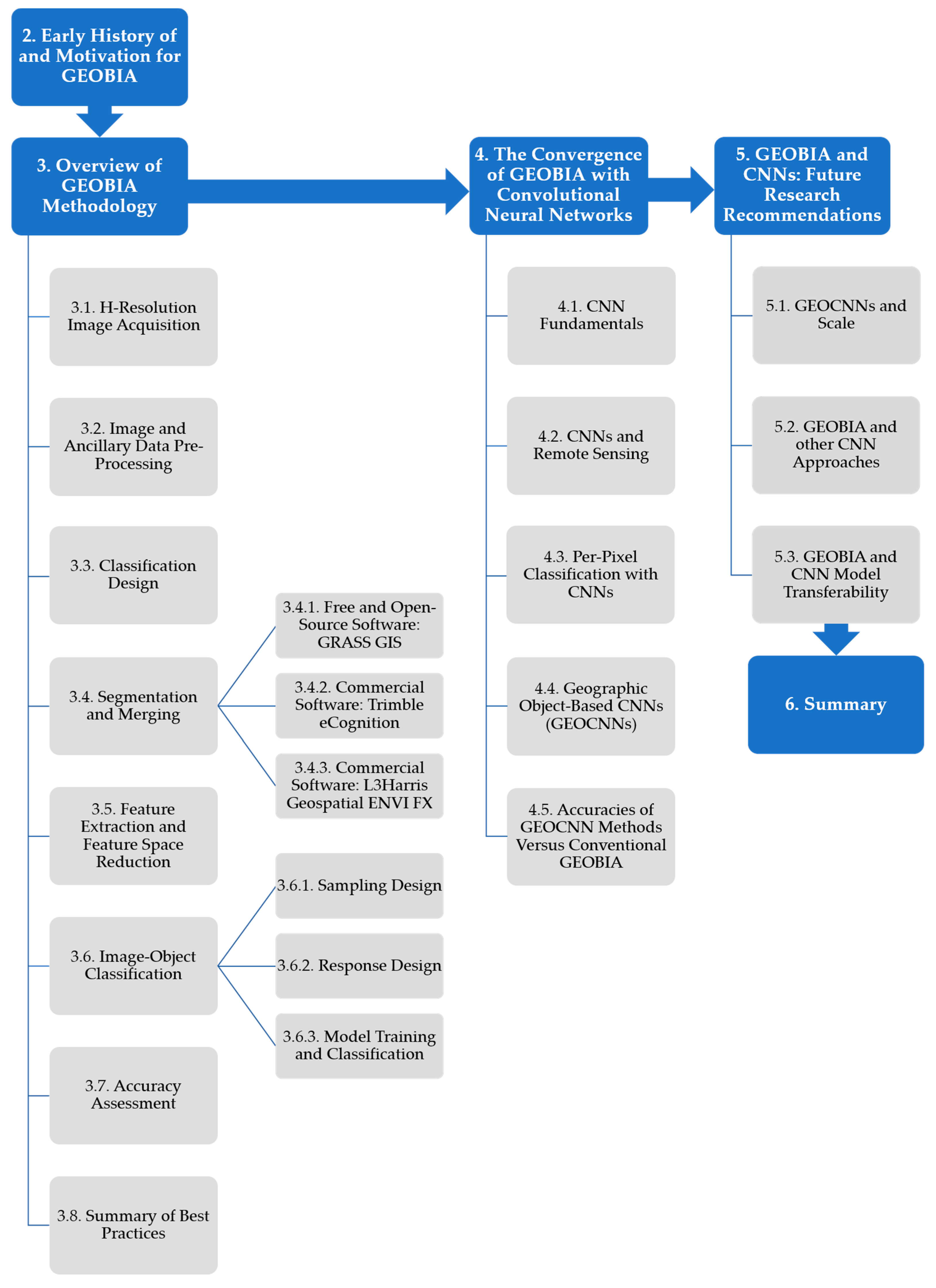
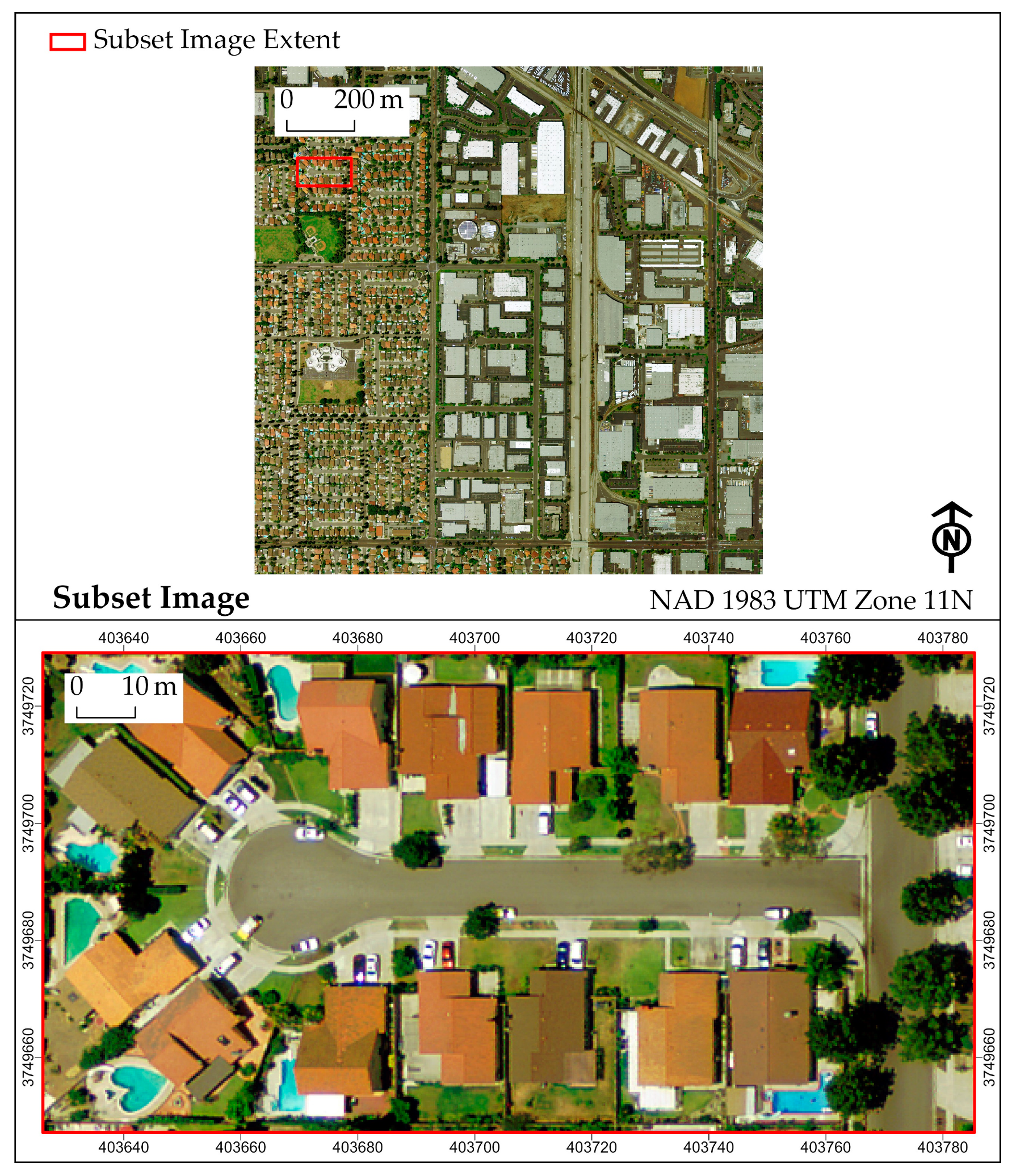
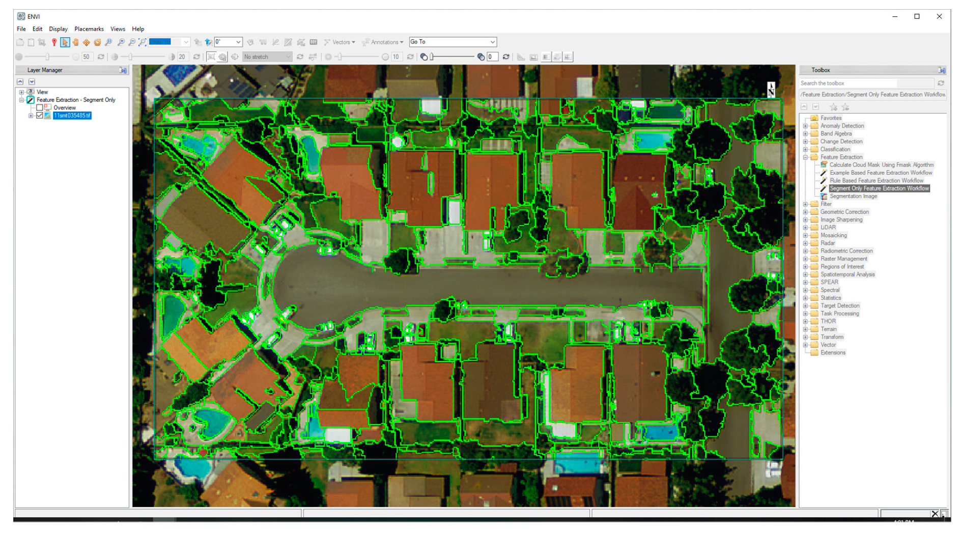
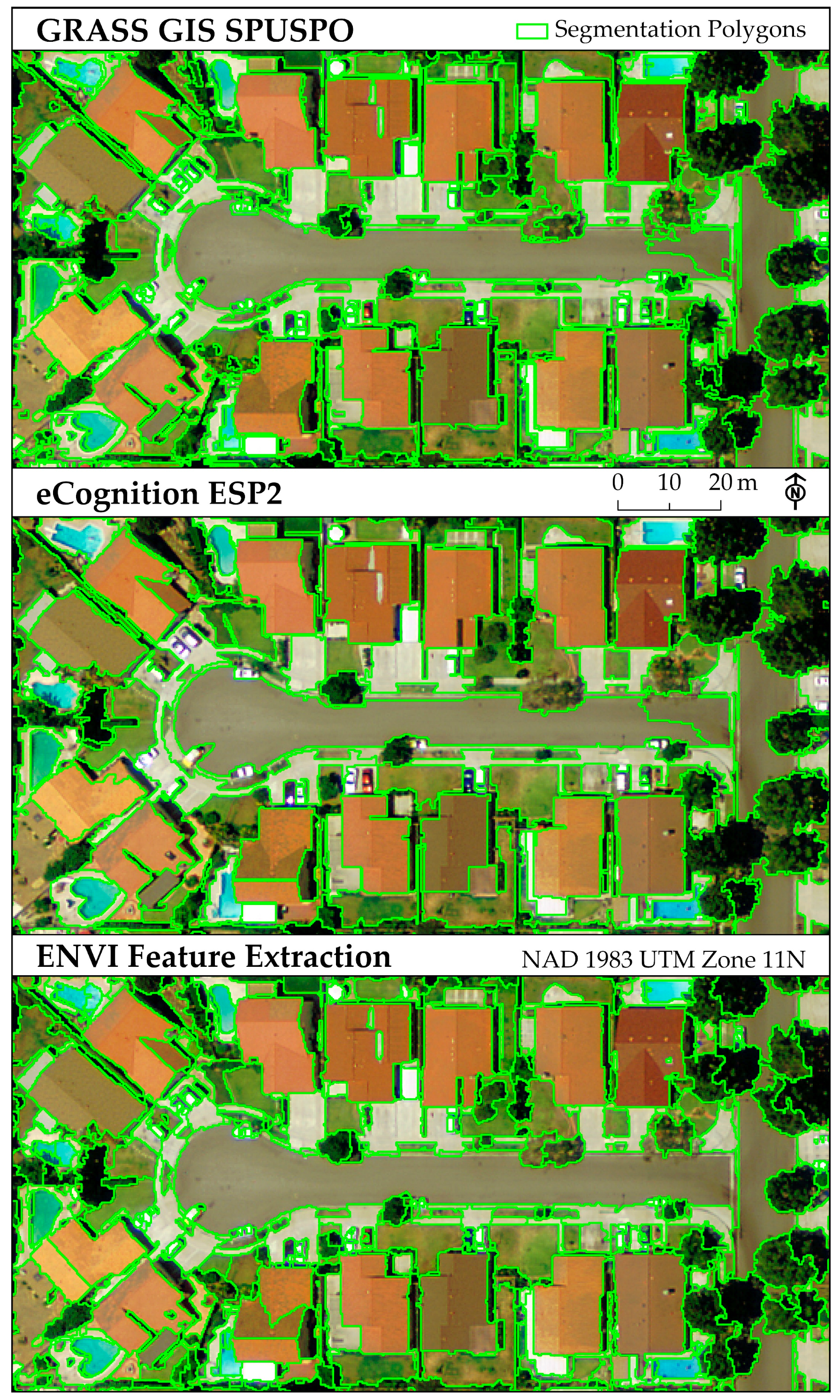
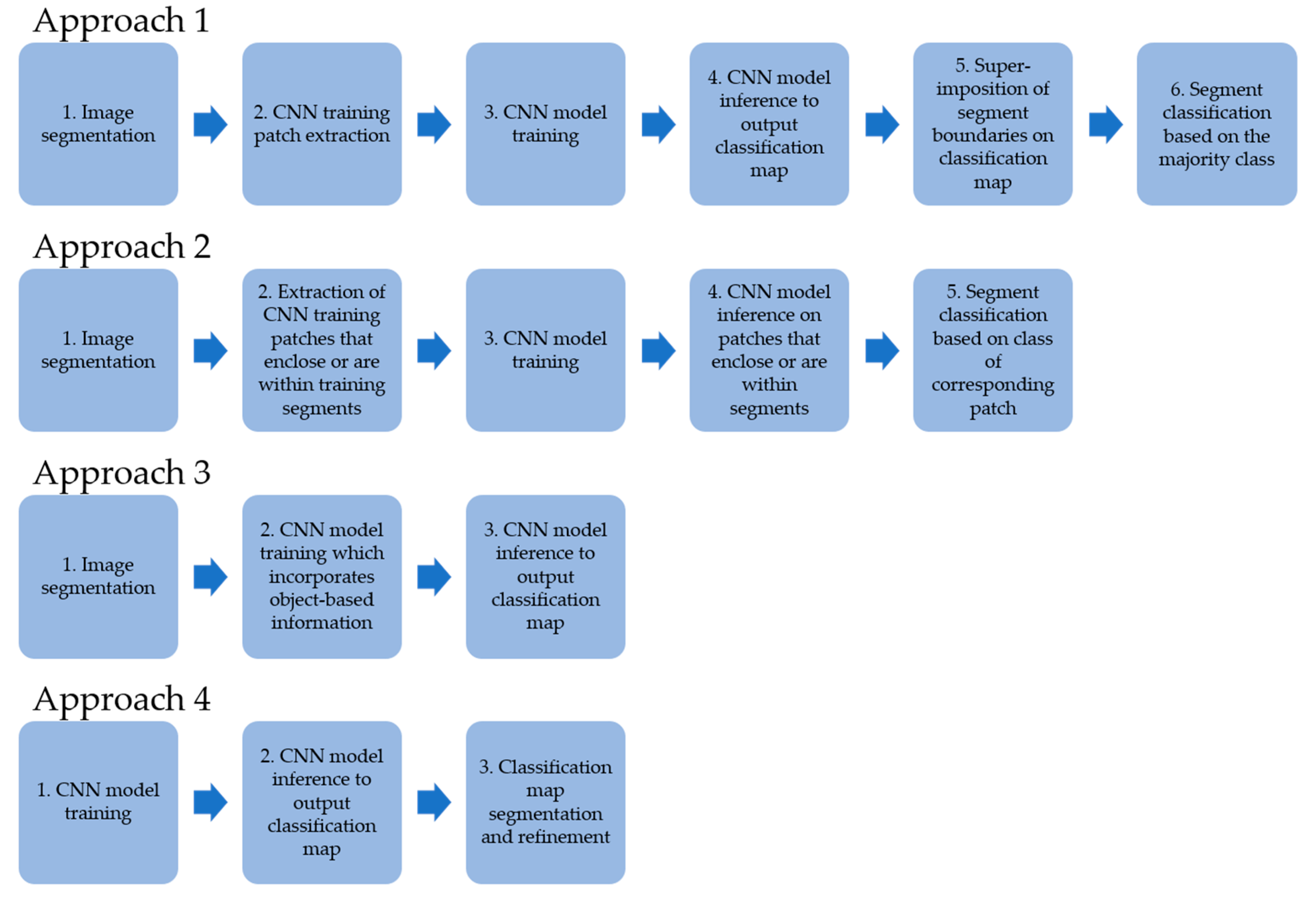
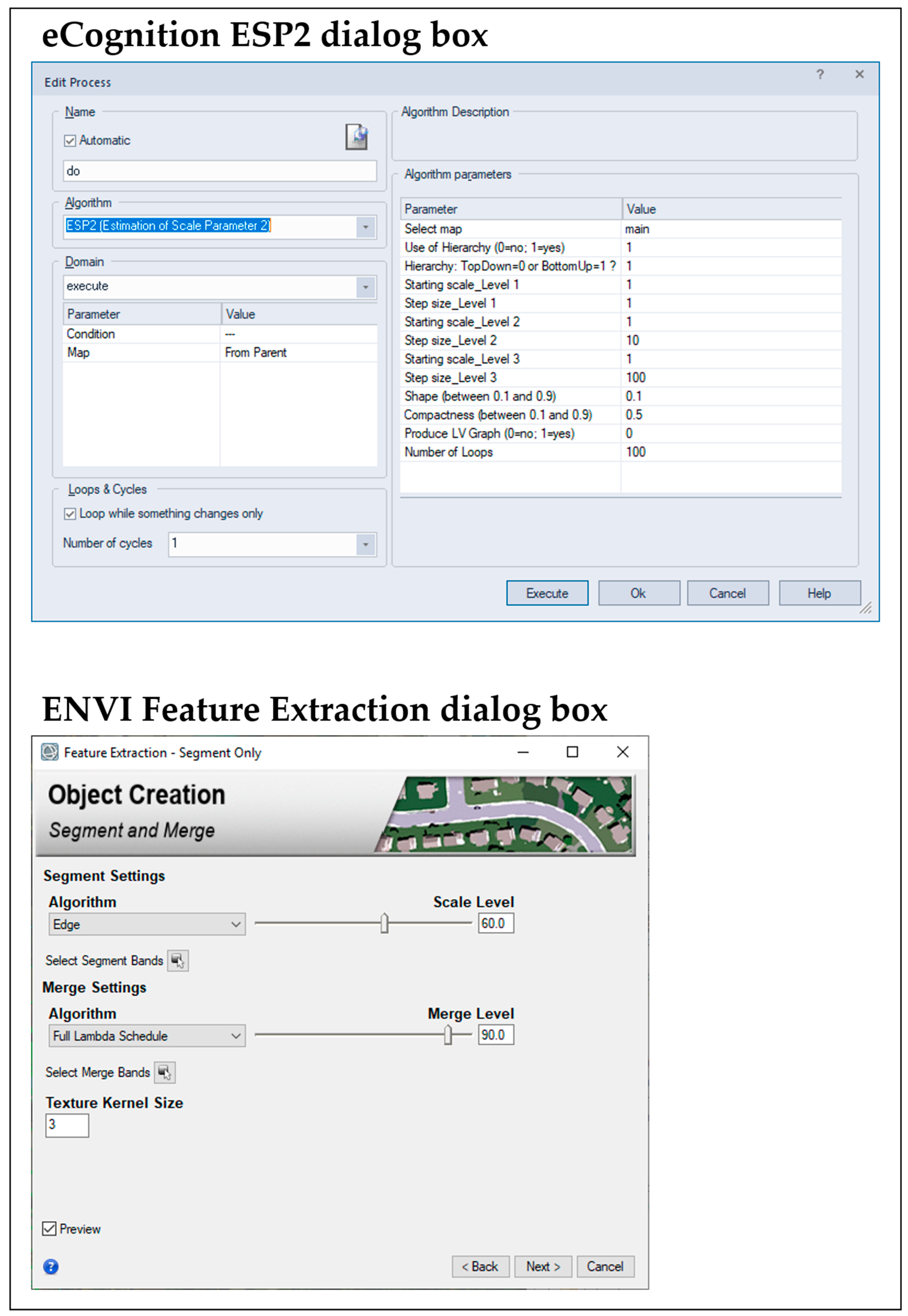
Table A1.
List of acronyms.
| Acronym | Meaning |
|---|---|
| CNN | convolutional neural network |
| DSM | digital surface model |
| DT | decision tree |
| DTM | digital terrain model |
| ESP2 | Estimation of Scale Parameter 2 |
| FCN | fully convolutional network |
| FSO | feature space optimization |
| GEOBIA | geographic object-based image analysis |
| GEOCNN | geographic object-based convolutional neural network |
| GIS | geographic information system |
| GIScience | geographic information science |
| KNN | k-nearest neighbors |
| LV | local variance |
| Mask R-CNN | Mask Region-based CNN |
| MAUP | modifiable areal unit problem |
| MI | Moran’s I |
| MLC | maximum likelihood classification |
| MRS | multiresolution segmentation |
| nDSM | normalized digital surface model |
| NN | nearest neighbor |
| OBIA | object-based image analysis |
| RF | random forest |
| SPUSPO | spatially partitioned unsupervised segmentation parameter optimization |
| SVM | support vector machine |
| TP | threshold parameter |
| VSURF | variable selection with random forests |
| WV | weighted variance |
Figure A1.
eCognition ESP2 dialog box (default settings) and ENVI Feature Extraction dialog box.

References
- Hay, G.J.; Castilla, G. Geographic object-based image analysis (GEOBIA): A new name for a new discipline. In Object-Based Image Analysis: Spatial Concepts for Knowledge-Driven Remote Sensing Applications; Blaschke, T., Lang, S., Hay, G.J., Eds.; Springer: Berlin, Germany, 2008; pp. 75–89. [Google Scholar]
- Blaschke, T.; Hay, G.J.; Kelly, M.; Lang, S.; Hofmann, P.; Addink, E.; Queiroz Feitosa, R.; van der Meer, F.; van der Werff, H.; van Coillie, F.; et al. Geographic Object-Based Image Analysis—Towards a new paradigm. ISPRS J. Photogramm. Remote Sens. 2014, 87, 180–191. [Google Scholar] [CrossRef] [PubMed] [Green Version]
- Radoux, J.; Bogaert, P. Good Practices for Object-Based Accuracy Assessment. Remote Sens. 2017, 9, 646. [Google Scholar] [CrossRef] [Green Version]
- Ma, L.; Li, M.; Ma, X.; Cheng, L.; Du, P.; Liu, Y. A review of supervised object-based land-cover image classification. ISPRS J. Photogramm. Remote Sens. 2017, 130, 277–293. [Google Scholar] [CrossRef]
- Castilla, G.; Hay, G.J. Image objects and geographic objects. In Object-Based Image Analysis: Spatial Concepts for Knowledge-Driven Remote Sensing Applications; Blaschke, T., Lang, S., Hay, G.J., Eds.; Springer: Berlin, Germany, 2008; pp. 91–110. [Google Scholar]
- Ye, S.; Pontius, R.G.; Rakshit, R. A review of accuracy assessment for object-based image analysis: From per-pixel to per-polygon approaches. ISPRS J. Photogramm. Remote Sens. 2018, 141, 137–147. [Google Scholar] [CrossRef]
- Hossain, M.D.; Chen, D. Segmentation for Object-Based Image Analysis (OBIA): A review of algorithms and challenges from remote sensing perspective. ISPRS J. Photogramm. Remote Sens. 2019, 150, 115–134. [Google Scholar] [CrossRef]
- Zhu, X.X.; Tuia, D.; Mou, L.; Xia, G.-S.; Zhang, L.; Xu, F.; Fraundorfer, F. Deep Learning in Remote Sensing: A Comprehensive Review and List of Resources. IEEE Geosci. Remote Sens. Mag. 2017, 5, 8–36. [Google Scholar] [CrossRef] [Green Version]
- Ma, L.; Liu, Y.; Zhang, X.; Ye, Y.; Yin, G.; Johnson, B.A. Deep learning in remote sensing applications: A meta-analysis and review. ISPRS J. Photogramm. Remote Sens. 2019, 152, 166–177. [Google Scholar] [CrossRef]
- Lang, S.; Hay, G.J.; Baraldi, A.; Tiede, D.; Blaschke, T. GEOBIA Achievements and Spatial Opportunities in the Era of Big Earth Observation Data. ISPRS Int. J. Geo-Inf. 2019, 8, 474. [Google Scholar] [CrossRef] [Green Version]
- Hay, G.J.; Niemann, K.O. Visualizing 3-D Texture: A Three-Dimensional Structural Approach to Model Forest Texture. Can. J. Remote Sens. 1994, 20, 90–101. [Google Scholar]
- Hay, G.J.; Niemann, K.O.; McLean, G.F. An object-specific image-texture analysis of H-resolution forest imagery. Remote Sens. Environ. 1996, 55, 108–122. [Google Scholar] [CrossRef]
- Marceau, D.J.; Howarth, P.J.; Dubois, J.M.M.; Gratton, D.J. Evaluation of the Grey-Level Co-Occurrence Matrix Method for Land-Cover Classification Using SPOT Imagery. IEEE Trans. Geosci. Remote Sens. 1990, 28, 513–519. [Google Scholar] [CrossRef]
- Blaschke, T. Object based image analysis for remote sensing. ISPRS J. Photogramm. Remote Sens. 2010, 65, 2–16. [Google Scholar] [CrossRef] [Green Version]
- Hay, G.J.; Castilla, G.; Wulder, M.A.; Ruiz, J.R. An automated object-based approach for the multiscale image segmentation of forest scenes. Int. J. Appl. Earth Obs. Geoinf. 2005, 7, 339–359. [Google Scholar] [CrossRef]
- Strahler, A.H.; Woodcock, C.E.; Smith, J.A. On the Nature of Models in Remote Sensing. Remote Sens. Environ. 1986, 20, 121–139. [Google Scholar] [CrossRef]
- Lang, S. Object-based image analysis for remote sensing applications: Modeling reality—Dealing with complexity. In Object-Based Image Analysis: Spatial Concepts for Knowledge-Driven Remote Sensing Applications; Blaschke, T., Lang, S., Hay, G.J., Eds.; Springer: Berlin, Germany, 2008; pp. 3–27. [Google Scholar]
- Woodcock, C.E.; Strahler, A.H. The Factor of Scale in Remote Sensing. Remote Sens. Environ. 1987, 21, 311–332. [Google Scholar] [CrossRef]
- Blaschke, T.; Strobl, J. What’s wrong with pixels? Some recent developments interfacing remote sensing and GIS. Zeitschrift fur Geoinformationssysteme 2001, 14, 12–17. [Google Scholar]
- Fotheringham, A.S.; Wong, D.W.S. The modifiable areal unit problem in multivariate statistical analysis. Environ. Plan. A 1991, 23, 1025–1044. [Google Scholar] [CrossRef]
- Hay, G.J.; Blaschke, T.; Marceau, D.J.; Bouchard, A. A comparison of three image-object methods for the multiscale analysis of landscape structure. ISPRS J. Photogramm. Remote Sens 2003, 57, 327–345. [Google Scholar]
- Marceau, D.J.; Hay, G.J. Remote Sensing Contributions to the Scale Issue. Can. J. Remote Sens. 1999, 25, 357–366. [Google Scholar] [CrossRef]
- Hay, G.J.; Marceau, D.J. Multiscale Object-Specific Analysis (MOSA): An integrative approach for multiscale landscape analysis. In Remote Sensing Image Analysis: Including the Spatial Domain; de Jong, S.M., van der Meer, F.D., Eds.; Kluwer Academic Publishers: Dordrecht, The Netherlands, 2004; Volume 5, pp. 1–33. ISBN 1-4020-2559-9. [Google Scholar]
- Hay, G.J.; Marceau, D.J.; Dubé, P.; Bouchard, A. A multiscale framework for landscape analysis: Object-specific analysis and upscaling. Landsc. Ecol. 2001, 16, 471–490. [Google Scholar] [CrossRef]
- Drǎguţ, L.; Csillik, O.; Eisank, C.; Tiede, D. Automated parameterisation for multi-scale image segmentation on multiple layers. ISPRS J. Photogramm. Remote Sens. 2014, 88, 119–127. [Google Scholar] [CrossRef] [Green Version]
- Burnett, C.; Blaschke, T. A multi-scale segmentation/object relationship modelling methodology for landscape analysis. Ecol. Modell. 2003, 168, 233–249. [Google Scholar] [CrossRef]
- Chen, G.; Hay, G.J.; Carvalho, L.M.T.; Wulder, M.A. Object-based change detection. Int. J. Remote Sens. 2012, 33, 4434–4457. [Google Scholar] [CrossRef]
- Gerçek, D.; Toprak, V.; Stroblc, J. Object-based classification of landforms based on their local geometry and geomorphometric context. Int. J. Geogr. Inf. Sci. 2011, 25, 1011–1023. [Google Scholar] [CrossRef]
- Grippa, T.; Lennert, M.; Beaumont, B.; Vanhuysse, S.; Stephenne, N.; Wolff, E. An Open-Source Semi-Automated Processing Chain for Urban Object-Based Classification. Remote Sens. 2017, 9, 358. [Google Scholar] [CrossRef] [Green Version]
- Georganos, S.; Grippa, T.; Lennert, M.; Vanhuysse, S.; Johnson, B.A.; Wolff, E. Scale Matters: Spatially Partitioned Unsupervised Segmentation Parameter Optimization for Large and Heterogeneous Satellite Images. Remote Sens. 2018, 10, 1440. [Google Scholar] [CrossRef] [Green Version]
- Griffith, D.; Hay, G. Integrating GEOBIA, Machine Learning, and Volunteered Geographic Information to Map Vegetation over Rooftops. ISPRS Int. J. Geo-Information 2018, 7, 462. [Google Scholar] [CrossRef] [Green Version]
- L3Harris Geospatial. Extract Segments Only. Available online: https://www.harrisgeospatial.com/docs/segmentonly.html (accessed on 17 April 2020).
- Chen, G.; Weng, Q.; Hay, G.J.; He, Y. Geographic object-based image analysis (GEOBIA): Emerging trends and future opportunities. GIScience Remote Sens. 2018, 55, 159–182. [Google Scholar] [CrossRef]
- Baatz, M.; Hoffmann, C.; Willhauck, G. Progressing from object-based to object-oriented image analysis. In Object-Based Image Analysis: Spatial Concepts for Knowledge-Driven Remote Sensing Applications; Blaschke, T., Lang, S., Hay, G.J., Eds.; Springer: Berlin, Germany, 2008; pp. 29–42. [Google Scholar]
- L3Harris Geospatial. Merge Algorithms Background. Available online: https://www.harrisgeospatial.com/docs/backgroundmergealgorithms.html (accessed on 17 April 2020).
- Ma, L.; Cheng, L.; Li, M.; Liu, Y.; Ma, X. Training set size, scale, and features in Geographic Object-Based Image Analysis of very high resolution unmanned aerial vehicle imagery. ISPRS J. Photogramm. Remote Sens. 2015, 102, 14–27. [Google Scholar] [CrossRef]
- Li, M.; Ma, L.; Blaschke, T.; Cheng, L.; Tiede, D. A systematic comparison of different object-based classification techniques using high spatial resolution imagery in agricultural environments. Int. J. Appl. Earth Obs. Geoinf. 2016, 49, 87–98. [Google Scholar] [CrossRef]
- Hanbury, A. Image Segmentation by Region Based and Watershed Algorithms. Wiley Encycl. Comput. Sci. Eng. 2008, 1543–1552. [Google Scholar]
- Leibniz Institute of Ecological Urban and Regional Development. Segmentation Evaluation. Available online: https://www.ioer.de/segmentation-evaluation/results.html (accessed on 17 April 2020).
- Orfeo ToolBox—Orfeo ToolBox is Not a BLACK box. Available online: https://www.orfeo-toolbox.org/ (accessed on 17 April 2020).
- InterIMAGE—Interpreting Images Freely. Available online: http://www.lvc.ele.puc-rio.br/projects/interimage/ (accessed on 17 April 2020).
- The Remote Sensing and GIS Software Library (RSGISLib). Available online: https://www.rsgislib.org/ (accessed on 17 April 2020).
- eCognition. Trimble Geospatial. Available online: https://geospatial.trimble.com/products-and-solutions/ecognition (accessed on 17 April 2020).
- ENVI—The Leading Geospatial Image Analysis Software. Available online: https://www.harrisgeospatial.com/Software-Technology/ENVI (accessed on 17 April 2020).
- ArcGIS Pro. 2D and 3D GIS Mapping Software—Esri. Available online: https://www.esri.com/en-us/arcgis/products/arcgis-pro/overview (accessed on 17 April 2020).
- PCI Geomatica. Available online: https://www.pcigeomatics.com/software/geomatica/professional (accessed on 17 April 2020).
- Momsen, E.; Metz, M. GRASS GIS Manual: I.segment. Available online: https://grass.osgeo.org/grass74/manuals/i.segment.html (accessed on 17 April 2020).
- Lennert, M. GRASS GIS Manual: I.cutlines. Available online: https://grass.osgeo.org/grass78/manuals/addons/i.cutlines.html (accessed on 17 April 2020).
- Lennert, M. GRASS GIS Manual: I.segment.uspo. Available online: https://grass.osgeo.org/grass78/manuals/addons/i.segment.uspo.html (accessed on 17 April 2020).
- Baatz, M.; Schäpe, A. Multiresolution Segmentation: An optimization approach for high quality multi-scale image segmentation. In Angewandte Geographische Informationsverarbeitung XII; Strobl, J., Blaschke, T., Griesebner, G., Eds.; Salzburg Geographical Materials: Salzburg, Austria, 2000; pp. 12–23. [Google Scholar]
- Trimble. Reference Book: Trimble eCognition Developer for Windows operating system; Trimble Germany GmbH: Munich, Germany, 2017; ISBN 2008000834. [Google Scholar]
- Drǎguţ, L.; Tiede, D.; Levick, S.R. ESP: A tool to estimate scale parameter for multiresolution image segmentation of remotely sensed data. Int. J. Geogr. Inf. Sci. 2010, 24, 859–871. [Google Scholar] [CrossRef]
- Zhang, X.; Xiao, P.; Feng, X. Object-specific optimization of hierarchical multiscale segmentations for high-spatial resolution remote sensing images. ISPRS J. Photogramm. Remote Sens. 2020, 159, 308–321. [Google Scholar] [CrossRef]
- L3Harris Geospatial. Segmentation Algorithms Background. Available online: https://www.harrisgeospatial.com/docs/backgroundsegmentationalgorithm.html (accessed on 17 April 2020).
- USGS. High Resolution Orthoimagery, Los Angeles County, California, USA, Entity ID: 3527226_11SMT035485. Available online: https://earthexplorer.usgs.gov/ (accessed on 17 April 2020).
- L3Harris Geospatial. List of Attributes. Available online: https://www.harrisgeospatial.com/docs/attributelist.html (accessed on 24 May 2020).
- Haralick, R.M. Statistical and structural approaches to texture. Proc. IEEE 1979, 67, 786–804. [Google Scholar] [CrossRef]
- Haralick, R.M.; Shanmugam, K.; Dinstein, I. Textural Features for Image Classification. IEEE Trans. Syst. Man. Cybern. 1973, SMC-3, 610–621. [Google Scholar]
- Hall-Beyer, M. Practical guidelines for choosing GLCM textures to use in landscape classification tasks over a range of moderate spatial scales. Int. J. Remote Sens. 2017, 38, 1312–1338. [Google Scholar] [CrossRef]
- Ma, L.; Fu, T.; Tiede, D.; Blaschke, T.; Ma, X.; Chen, D.; Zhou, Z.; Li, M. Evaluation of Feature Selection Methods for Object-Based Land Cover Mapping of Unmanned Aerial Vehicle Imagery Using Random Forest and Support Vector Machine Classifiers. ISPRS Int. J. Geo-Inf. 2017, 6, 51. [Google Scholar] [CrossRef]
- L3Harris Geospatial. Example-Based Classification. Available online: https://www.harrisgeospatial.com/docs/example_based_classification.html (accessed on 17 April 2020).
- L3Harris Geospatial. An Interval Based Attribute Ranking Technique; L3Harris Geospatial: Boulder, CO, USA, 2007. [Google Scholar]
- Genuer, R.; Poggi, J.-M.; Tuleau-Malot, C. VSURF: An R Package for Variable Selection Using Random Forests. R J. 2015, 7, 19–33. [Google Scholar] [CrossRef] [Green Version]
- Genuer, R.; Poggi, J.-M.; Tuleau-Malot, C. Variable selection using random forests. Pattern Recognit. Lett. 2010, 31, 2225–2236. [Google Scholar] [CrossRef] [Green Version]
- Maxwell, A.E.; Strager, M.P.; Warner, T.A.; Ramezan, C.A.; Morgan, A.N.; Pauley, C.E. Large-Area, High Spatial Resolution Land Cover Mapping Using Random Forests, GEOBIA, and NAIP Orthophotography: Findings and Recommendations. Remote Sens. 2019, 11, 1409. [Google Scholar] [CrossRef] [Green Version]
- Millard, K.; Richardson, M. On the importance of training data sample selection in Random Forest image classification: A case study in peatland ecosystem mapping. Remote Sens. 2015, 7, 8489–8515. [Google Scholar] [CrossRef] [Green Version]
- Perlich, C.; Simonoff, J.S. Tree Induction vs. Logistic Regression: A Learning-Curve Analysis. J. Mach. Learn. Res. 2003, 4, 211–255. [Google Scholar]
- Müller, A.C.; Guido, S. Introduction to Machine Learning with Python; O’Reilly Media: Sebastopol, CA, USA, 2017; ISBN 9781449369903. [Google Scholar]
- Maxwell, A.E.; Warner, T.A.; Fang, F. Implementation of machine-learning classification in remote sensing: An applied review. Int. J. Remote Sens. 2018, 39, 2784–2817. [Google Scholar] [CrossRef] [Green Version]
- Stehman, S.V.; Foody, G.M. Key issues in rigorous accuracy assessment of land cover products. Remote Sens. Environ. 2019, 231, 1–23. [Google Scholar] [CrossRef]
- Whiteside, T.G.; Maier, S.W.; Boggs, G.S. Area-based and location-based validation of classified image objects. Int. J. Appl. Earth Obs. Geoinf. 2014, 28, 117–130. [Google Scholar] [CrossRef]
- Osmólska, A.; Hawryło, P. Using a GEOBIA framework for integrating different data sources and classification methods in context of land use/land cover mapping. Geod. Cartogr. 2018, 67, 99–116. [Google Scholar]
- Liu, X.H.; Skidmore, A.K.; Van Oosten, H. Integration of classification methods for improvement of land-cover map accuracy. ISPRS J. Photogramm. Remote Sens. 2002, 56, 257–268. [Google Scholar] [CrossRef]
- Belgiu, M.; Drǎguţ, L.; Strobl, J. Quantitative evaluation of variations in rule-based classifications of land cover in urban neighbourhoods using WorldView-2 imagery. ISPRS J. Photogramm. Remote Sens. 2014, 87, 205–215. [Google Scholar] [CrossRef] [Green Version]
- Mountrakis, G.; Im, J.; Ogole, C. Support vector machines in remote sensing: A review. ISPRS J. Photogramm. Remote Sens. 2011, 66, 247–259. [Google Scholar] [CrossRef]
- Breiman, L. Random forests. Mach. Learn. 2001, 45, 5–32. [Google Scholar] [CrossRef] [Green Version]
- Strobl, C.; Malley, J.; Tutz, G. An Introduction to Recursive Partitioning: Rationale, Application, and Characteristics of Classification and Regression Trees, Bagging, and Random Forests. Psychol. Methods 2009, 14, 323–348. [Google Scholar] [CrossRef] [Green Version]
- Belgiu, M.; Drăguţ, L. Random forest in remote sensing: A review of applications and future directions. ISPRS J. Photogramm. Remote Sens. 2016, 114, 24–31. [Google Scholar] [CrossRef]
- Chollet, F. Deep Learning with Python; Manning Publications Co.: Shelter Island, NY, USA, 2018; ISBN 9781617294433. [Google Scholar]
- Pontius, R.G., Jr.; Millones, M. Death to Kappa: Birth of quantity disagreement and allocation disagreement for accuracy assessment. Int. J. Remote Sens. 2011, 32, 4407–4429. [Google Scholar] [CrossRef]
- Liu, C.; Frazier, P.; Kumar, L. Comparative assessment of the measures of thematic classification accuracy. Remote Sens. Environ. 2007, 107, 606–616. [Google Scholar] [CrossRef]
- L3Harris Geospatial. Calculate Confusion Matrices. Available online: https://www.harrisgeospatial.com/docs/CalculatingConfusionMatrices.html (accessed on 17 April 2020).
- Trimble. eCognition Developer: Tutorial 6—Working with the Accuracy Assessment Tool. Available online: https://docs.ecognition.com/v9.5.0/Resources/Images/Tutorial%206%20-%20Accuracy%20Assessment%20Tool.pdf (accessed on 17 April 2020).
- Cai, L.; Shi, W.; Miao, Z.; Hao, M. Accuracy Assessment Measures for Object Extraction from Remote Sensing Images. Remote Sens. 2018, 10, 303. [Google Scholar] [CrossRef] [Green Version]
- Chartrand, G.; Cheng, P.M.; Vorontsov, E.; Drozdzal, M.; Turcotte, S.; Pal, C.J.; Kadoury, S.; Tang, A. Deep learning: A primer for radiologists. Radiographics 2017, 37, 2113–2131. [Google Scholar] [CrossRef] [PubMed] [Green Version]
- LeCun, Y.; Bengio, Y.; Hinton, G. Deep learning. Nature 2015, 521, 436–444. [Google Scholar] [CrossRef]
- Yamashita, R.; Nishio, M.; Do, R.K.G.; Togashi, K. Convolutional neural networks: An overview and application in radiology. Insights Imaging 2018, 9, 611–629. [Google Scholar] [CrossRef] [Green Version]
- Zhang, L.; Zhang, L.; Du, B. Deep Learning for Remote Sensing Data: A Technical Tutorial on the State of the Art. IEEE Geosci. Remote Sens. Mag. 2016, 4, 22–40. [Google Scholar] [CrossRef]
- Cheng, G.; Han, J.; Lu, X. Remote Sensing Image Scene Classification: Benchmark and State of the Art. Proc. IEEE 2017, 105, 1865–1883. [Google Scholar] [CrossRef] [Green Version]
- Ball, J.E.; Anderson, D.T.; Chan, C.S. A Comprehensive Survey of Deep Learning in Remote Sensing: Theories, Tools and Challenges for the Community. J. Appl. Remote Sens. 2017, 11, 1–54. [Google Scholar] [CrossRef] [Green Version]
- Li, Y.; Zhang, H.; Xue, X.; Jiang, Y.; Shen, Q. Deep learning for remote sensing image classification: A survey. Wiley Interdiscip. Rev. Data Min. Knowl. Discov. 2018, 8, 1–17. [Google Scholar]
- Fu, T.; Ma, L.; Li, M.; Johnson, B.A. Using convolutional neural network to identify irregular segmentation objects from very high-resolution remote sensing imagery. J. Appl. Remote Sens. 2018, 12, 1–21. [Google Scholar] [CrossRef]
- Litjens, G.; Kooi, T.; Bejnordi, B.E.; Setio, A.A.A.; Ciompi, F.; Ghafoorian, M.; van der Laak, J.A.W.M.; van Ginneken, B.; Sánchez, C.I. A survey on deep learning in medical image analysis. Med. Image Anal. 2017, 42, 60–88. [Google Scholar] [CrossRef] [PubMed] [Green Version]
- Pasupa, K.; Sunhem, W. A comparison between shallow and deep architecture classifiers on small dataset. In Proceedings of the International Conference on Information Technology and Electrical Engineering, Yogyakarta, Indonesia, 5–6 October 2016. [Google Scholar]
- Hay, G.J. Visualizing Scale-Domain Manifolds: A Multiscale Geo-Object-Based Approach. In Scale Issues in Remote Sensing; Weng, Q., Ed.; John Wiley & Sons, Inc.: Hoboken, NJ, USA, 2014; pp. 141–169. ISBN 978-1-118-30504-1. [Google Scholar]
- Li, Y.; Ye, S.; Bartoli, I. Semisupervised classification of hurricane damage from postevent aerial imagery using deep learning. J. Appl. Remote Sens. 2018, 12, 1–13. [Google Scholar] [CrossRef]
- Vetrivel, A.; Gerke, M.; Kerle, N.; Nex, F.; Vosselman, G. Disaster damage detection through synergistic use of deep learning and 3D point cloud features derived from very high resolution oblique aerial images, and multiple-kernel-learning. ISPRS J. Photogramm. Remote Sens. 2018, 140, 45–59. [Google Scholar] [CrossRef]
- Jozdani, S.E.; Johnson, B.A.; Chen, D. Comparing Deep Neural Networks, Ensemble Classifiers, and Support Vector Machine Algorithms for Object-Based Urban Land Use/Land Cover Classification. Remote Sens. 2019, 11, 1713. [Google Scholar] [CrossRef] [Green Version]
- Maggiori, E.; Tarabalka, Y.; Charpiat, G.; Alliez, P. Convolutional Neural Networks for Large-Scale Remote-Sensing Image Classification. IEEE Trans. Geosci. Remote Sens. 2017, 55, 645–657. [Google Scholar] [CrossRef] [Green Version]
- Zhao, W.; Du, S.; Emery, W.J. Object-Based Convolutional Neural Network for High-Resolution Imagery Classification. IEEE J. Sel. Top. Appl. Earth Obs. Remote Sens. 2017, 10, 3386–3396. [Google Scholar] [CrossRef]
- Zhang, C.; Sargent, I.; Pan, X.; Li, H.; Gardiner, A.; Hare, J.; Atkinson, P.M. An object-based convolutional neural network (OCNN) for urban land use classification. Remote Sens. Environ. 2018, 216, 57–70. [Google Scholar] [CrossRef] [Green Version]
- Mboga, N.; Georganos, S.; Grippa, T.; Lennert, M.; Vanhuysse, S.; Wolff, E. Fully Convolutional Networks and Geographic Object-Based Image Analysis for the Classification of VHR Imagery. Remote Sens. 2019, 11, 597. [Google Scholar] [CrossRef] [Green Version]
- Chen, Y.; Ming, D.; Lv, X. Superpixel based land cover classification of VHR satellite image combining multi-scale CNN and scale parameter estimation. Earth Sci. Inform. 2019, 12, 341–363. [Google Scholar] [CrossRef]
- Davari Majd, R.; Momeni, M.; Moallem, P. Transferable Object-Based Framework Based on Deep Convolutional Neural Networks for Building Extraction. IEEE J. Sel. Top. Appl. Earth Obs. Remote Sens. 2019, 12, 2627–2635. [Google Scholar] [CrossRef]
- Papadomanolaki, M.; Vakalopoulou, M.; Karantzalos, K. A Novel Object-Based Deep Learning Framework for Semantic Segmentation of Very High-Resolution Remote Sensing Data: Comparison with Convolutional and Fully Convolutional Networks. Remote Sens. 2019, 11, 684. [Google Scholar] [CrossRef] [Green Version]
- Huang, H.; Lan, Y.; Yang, A.; Zhang, Y.; Wen, S.; Deng, J. Deep learning versus Object-based Image Analysis (OBIA) in weed mapping of UAV imagery. Int. J. Remote Sens. 2020, 41, 3446–3479. [Google Scholar] [CrossRef]
- Long, J.; Shelhamer, E.; Darrell, T. Fully Convolutional Networks for Semantic Segmentation. In Proceedings of the IEEE Conference on Computer Vision and Pattern Recognition, Boston, MA, USA, 7–12 June 2015; pp. 3431–3440. [Google Scholar]
- Prakash, N.; Manconi, A.; Loew, S. Mapping Landslides on EO Data: Performance of Deep Learning Models vs. Traditional Machine Learning Models. Remote Sens. 2020, 12, 346. [Google Scholar] [CrossRef] [Green Version]
- Liu, T.; Abd-Elrahman, A.; Morton, J.; Wilhelm, V.L. Comparing fully convolutional networks, random forest, support vector machine, and patch-based deep convolutional neural networks for object-based wetland mapping using images from small unmanned aircraft system. GISci. Remote Sens. 2018, 55, 243–264. [Google Scholar] [CrossRef]
- Liu, S.; Qi, Z.; Li, X.; Yeh, A. Integration of Convolutional Neural Networks and Object-Based Post-Classification Refinement for Land Use and Land Cover Mapping with Optical and SAR Data. Remote Sens. 2019, 11, 690. [Google Scholar] [CrossRef] [Green Version]
- Feng, W.; Sui, H.; Hua, L.; Xu, C. Improved Deep Fully Convolutional Network with Superpixel-Based Conditional Random Fields for Building Extraction. Int. Geosci. Remote Sens. Symp. 2019, 52–55. [Google Scholar]
- Zhou, K.; Ming, D.; Lv, X.; Fang, J.; Wang, M. CNN-based land cover classification combining stratified segmentation and fusion of point cloud and very high-spatial resolution remote sensing image data. Remote Sens. 2019, 11, 2065. [Google Scholar] [CrossRef] [Green Version]
- Song, D.; Tan, X.; Wang, B.; Zhang, L.; Shan, X.; Cui, J. Integration of super-pixel segmentation and deep-learning methods for evaluating earthquake-damaged buildings using single-phase remote sensing imagery. Int. J. Remote Sens. 2020, 41, 1040–1066. [Google Scholar] [CrossRef]
- Sothe, C.; De Almeida, C.M.; Schimalski, M.B.; Liesenberg, V.; La Rosa, L.E.C.; Castro, J.D.B.; Feitosa, R.Q. A comparison of machine and deep-learning algorithms applied to multisource data for a subtropical forest area classification. Int. J. Remote Sens. 2019, 41, 1943–1969. [Google Scholar] [CrossRef]
- Zhang, X.; Wang, Q.; Chen, G.; Dai, F.; Zhu, K.; Gong, Y.; Xie, Y. An object-based supervised classification framework for very-high-resolution remote sensing images using convolutional neural networks. Remote Sens. Lett. 2018, 9, 373–382. [Google Scholar] [CrossRef]
- Poomani Alias Punitha, M.; Sutha, J. Object based classification of high resolution remote sensing image using HRSVM-CNN classifier. Eur. J. Remote Sens. 2019. [Google Scholar] [CrossRef] [Green Version]
- Timilsina, S.; Sharma, S.K.; Aryal, J. Mapping Urban Trees Within Cadastral Parcels Using an Object-based Convolutional Neural Network. ISPRS Ann. Photogramm. Remote Sens. Spat. Inf. Sci. 2019, IV-5/W2, 111–117. [Google Scholar] [CrossRef] [Green Version]
- He, K.; Gkioxari, G.; Dollár, P.; Girshick, R. Mask R-CNN. In Proceedings of the IEEE International Conference on Computer Vision, Venice, Italy, 22–29 October 2017; pp. 2980–2988. [Google Scholar]
- Zhang, W.; Witharana, C.; Liljedahl, A.K.; Kanevskiy, M. Deep Convolutional Neural Networks for Automated Characterization of Arctic Ice-Wedge Polygons in Very High Spatial Resolution Aerial Imagery. Remote Sens. 2018, 10, 1487. [Google Scholar] [CrossRef] [Green Version]
- Zhao, K.; Kang, J.; Jung, J.; Sohn, G.; Street, K.; Drive, M.; York, N.; Mb, O.N. Building Extraction from Satellite Images Using Mask R-CNN with Building Boundary Regularization. In Proceedings of the IEEE Conference on Computer Vision and Pattern Recognition Workshops, Salt Lake City, UT, USA, 18–22 June 2018; pp. 247–251. [Google Scholar]
- Ji, S.; Wei, S.; Lu, M. Fully Convolutional Networks for Multisource Building Extraction from an Open Aerial and Satellite Imagery Data Set. IEEE Trans. Geosci. Remote Sens. 2019, 57, 574–586. [Google Scholar] [CrossRef]
- Ji, S.; Shen, Y.; Lu, M.; Zhang, Y. Building Instance Change Detection from Large-Scale Aerial Images using Convolutional Neural Networks and Simulated Samples. Remote Sens. 2019, 11, 1343. [Google Scholar] [CrossRef] [Green Version]
- Wen, Q.; Jiang, K.; Wang, W.; Liu, Q.; Guo, Q.; Li, L.; Wang, P. Automatic Building Extraction from Google Earth Images under Complex Backgrounds Based on Deep Instance Segmentation Network. Sensors (Switzerland) 2019, 19, 333. [Google Scholar] [CrossRef] [Green Version]
- Nie, S.; Jiang, Z.; Zhang, H.; Cai, B.; Yao, Y. Inshore Ship Detection Based on Mask R-CNN. Int. Geosci. Remote Sens. Symp. 2018, 693–696. [Google Scholar]
- Zhang, Y.; Zhang, Y.; Li, S.; Zhang, J. Accurate Detection of Berthing Ship Target Based on Mask R-CNN. In Proceedings of the International Conference on Image and Video Processing, and Artificial Intelligence, Shanghai, China, 15–17 August 2018; Volume 1083602, pp. 1–9. [Google Scholar]
- Feng, Y.; Diao, W.; Chang, Z.; Yan, M.; Sun, X.; Gao, X. Ship Instance Segmentation From Remote Sensing Images Using Sequence Local Context Module. In Proceedings of the IEEE International Geoscience and Remote Sensing Symposium, Yokohama, Japan, 28 July–2 August 2019; pp. 1025–1028. [Google Scholar]
- Zhao, T.; Yang, Y.; Niu, H.; Chen, Y.; Wang, D. Comparing U-Net convolutional networks with fully convolutional networks in the performances of pomegranate tree canopy segmentation. In Proceedings of the SPIE Asia-Pacific Remote Sensing Conference, Multispectral, Hyperspectral, Ultraspectral Remote Sensing Technology Techniques and Applications VII, Honolulu, HI, USA, 24–26 September 2018; Volume 10780, pp. 1–9. [Google Scholar]
- Krizhevsky, A.; Sutskever, I.; Hinton, G.E. ImageNet Classification with Deep Convolutional Neural Networks. In Proceedings of the Advances in Neural Information Processing Systems, Lake Tahoe, CA, USA, 3–8 December 2012; pp. 1–9. [Google Scholar]
- Guirado, E.; Tabik, S.; Alcaraz-Segura, D.; Cabello, J.; Herrera, F. Deep-learning Versus OBIA for scattered shrub detection with Google Earth Imagery: Ziziphus lotus as case study. Remote Sens. 2017, 9, 1220. [Google Scholar] [CrossRef] [Green Version]
- Bing. Microsoft Releases 18M Building Footprints in Uganda and Tanzania to Enable AI Assisted Mapping. Available online: https://blogs.bing.com/maps/2019-09/microsoft-releases-18M-building-footprints-in-uganda-and-tanzania-to-enable-ai-assisted-mapping (accessed on 17 April 2020).
- Bing. Microsoft Releases 12 million Canadian Building Footprints as Open Data. Available online: https://blogs.bing.com/maps/2019-03/microsoft-releases-12-million-canadian-building-footprints-as-open-data (accessed on 17 April 2020).
- Bing. Microsoft Releases 125 Million Building Footprints in the US as Open Data. Available online: https://blogs.bing.com/maps/2018-06/microsoft-releases-125-million-building-footprints-in-the-us-as-open-data (accessed on 17 April 2020).
- Duarte, D.; Nex, F.; Kerle, N.; Vosselman, G. Multi-resolution feature fusion for image classification of building damages with convolutional neural networks. Remote Sens. 2018, 10, 1636. [Google Scholar] [CrossRef] [Green Version]
Figure 1.
Flowchart overview showing the paper structure and organization.

Figure 2.
Remote sensing subset image used for the proceeding segmentation examples. Image source: USGS [55].
Figure 2.
Remote sensing subset image used for the proceeding segmentation examples. Image source: USGS [55].

Figure 3.
Near-real-time ENVI Feature Extraction segmentation preview (green polygons) that overlays the subset image. This segmentation preview can simply be dragged to a new location within the larger scene, which automatically applies the defined parameters (Figure A1) and segments the image-objects in the new location. Image source: USGS [55].

Figure 4.
Segmentation results for GRASS GIS SPUSPO, eCognition ESP2, and ENVI Feature Extraction. Image source: USGS [55].
Figure 4.
Segmentation results for GRASS GIS SPUSPO, eCognition ESP2, and ENVI Feature Extraction. Image source: USGS [55].

Figure 5.
Summaries of four geographic object-based CNN approaches.

| Spectral | Textural 1 | Geometrical | Contextual 2 |
|---|---|---|---|
| Mean | Homogeneity | Area | Length of shared border |
| Minimum | Contrast | Perimeter | Center-to-center distance |
| Maximum | Entropy | Elongation | Number of sub-objects |
Table 2.
Requirements and best practice recommendations for each methodological component 1.
| Methodological Section | Requirements and Recommendations |
|---|---|
| 3.1. H-Resolution Image Acquisition |
|
| 3.2. Image and Ancillary Data Pre-Processing |
|
| 3.3. Classification Design |
|
| 3.4. Segmentation and Merging |
|
| |
| 3.5. Feature Extraction and Feature Space Reduction |
|
| 3.6. Image-Object Classification |
|
| 3.7. Accuracy Assessment |
|
© 2020 by the authors. Licensee MDPI, Basel, Switzerland. This article is an open access article distributed under the terms and conditions of the Creative Commons Attribution (CC BY) license (http://creativecommons.org/licenses/by/4.0/).
Share and Cite
MDPI and ACS Style
Kucharczyk, M.; Hay, G.J.; Ghaffarian, S.; Hugenholtz, C.H. Geographic Object-Based Image Analysis: A Primer and Future Directions. Remote Sens. 2020, 12, 2012. https://0-doi-org.brum.beds.ac.uk/10.3390/rs12122012
AMA Style
Kucharczyk M, Hay GJ, Ghaffarian S, Hugenholtz CH. Geographic Object-Based Image Analysis: A Primer and Future Directions. Remote Sensing. 2020; 12(12):2012. https://0-doi-org.brum.beds.ac.uk/10.3390/rs12122012
Chicago/Turabian StyleKucharczyk, Maja, Geoffrey J. Hay, Salar Ghaffarian, and Chris H. Hugenholtz. 2020. "Geographic Object-Based Image Analysis: A Primer and Future Directions" Remote Sensing 12, no. 12: 2012. https://0-doi-org.brum.beds.ac.uk/10.3390/rs12122012
Note that from the first issue of 2016, this journal uses article numbers instead of page numbers. See further details here.