UAV Photogrammetry Accuracy Assessment for Corridor Mapping Based on the Number and Distribution of Ground Control Points

Abstract

Unmanned aerial vehicle (UAV) photogrammetry has recently emerged as a popular solution to obtain certain products necessary in linear projects, such as orthoimages or digital surface models. This is mainly due to its ability to provide these topographic products in a fast and economical way. In order to guarantee a certain degree of accuracy, it is important to know how many ground control points (GCPs) are necessary and how to distribute them across the study site. The purpose of this work consists of determining the number of GCPs and how to distribute them in a way that yields higher accuracy for a corridor-shaped study area. To do so, several photogrammetric projects have been carried out in which the number of GCPs used in the bundle adjustment and their distribution vary. The different projects were assessed taking into account two different parameters: the root mean square error (RMSE) and the Multiscale Model to Model Cloud Comparison (M3C2). From the different configurations tested, the projects using 9 and 11 GCPs (4.3 and 5.2 GCPs km⁻¹, respectively) distributed alternatively on both sides of the road in an offset or zigzagging pattern, with a pair of GCPs at each end of the road, yielded optimal results regarding fieldwork cost, compared to projects using similar or more GCPs placed according to other distributions.

1. Introduction

The availability of high-resolution topographic products, such as orthoimages and digital surface models (DSM), is of increasing importance for many different fields of engineering that require a thorough understanding of topographies. These include, among many others, terrain morphology to perform reliable simulation of soil erosion, flooding phenomena, and assessment of the sediment budget [1,2,3,4,5], landslide mapping and multi-temporal study [6,7,8], road design [9], road condition surveys for road management [10], precision agriculture [11], or detection of archaeological rests [12]. Unmanned aerial vehicles (UAV) have emerged as a feasible alternative given their lower cost, high temporal and spatial resolution, and flexibility in image acquisition compared to conventional airborne and satellite sensors [13,14,15]. Most available software applications currently used to process UAV-acquired imagery are based on the structure from motion (SfM) approach. This approach, unlike traditional digital photogrammetry, resolves the collinearity equations without the need for any control point, providing a sparse point cloud in an arbitrary coordinate system and a full camera calibration [16,17]. This is possible due to image matching algorithms that automatically search for similar image objects, called keypoints, through the analysis of the correspondence, similarity, and consistency of the image features [18]. SfM is paired with multi-view stereopsis (MVS) techniques that apply an expanding procedure of the sparse set of matched keypoints in order to obtain a dense point cloud [19].

To georeference the 3D point cloud generated in the photogrammetric process, ground control points (GCPs) are usually employed. These control points can be either permanent ground features or reference targets scattered on the ground before the flight, which must be surveyed to obtain their precise coordinates and ensure that they are clearly identifiable on the raw images. A minimum of three GCPs is necessary to carry out the georeferencing process, although increasing the number of GCPs is highly recommended in order to improve the accuracy of the photogrammetric products. In [20], the influence of the number of GCPs on the DSM and orthoimage accuracies obtained with UAV photogrammetry were studied. A similar conclusion for both horizontal and vertical components was derived: optimal results were reached with 15 GCPs. Furthermore, in [21], different numbers and distributions of GCPs were studied to try to optimize the products obtained by UAV photogrammetry on a surface of 22 ha: it was concluded that more accurate results were reached combining GCPs located around the study area and a stratified distribution inside that area. In [22], the effect of the number and distribution of GCPs on the accuracy of the DSM and orthophoto of a surface of 150 ha was studied. These last two studies reached similar conclusions, proposing 0.5 to 1 GCP ha⁻¹ as the optimum concentration of GCPs. In [23], the influence of different variations of GCPs arranged on an area of 2.73 ha on the accuracy of the products of UAV photogrammetry projects was studied. The optimum concentration was 1.8 GCPs ha⁻¹ uniformly distributed across the whole surface.

The 3D coordinates of GCPs must be accurate; thus, a suitable survey method, such as GPS or total stations, must be used. Surveying these points is a time-consuming task that can be difficult to carry out depending on the terrain morphology. Alternative to the use of GCPs, differential GPS (DGPS) correction techniques, such as real-time kinematics (RTKs) and post-processing kinematics (PPKs), have been evaluated as methods to provide high-accuracy georeferencing [24,25,26]. In [25], it was concluded that a UAV RTK/PPK solution can provide highly accurate spatial data (planimetric RMSE = 0.044 m, altimetric RMSE = 0.082 m), compared to data acquired through the use of GCPs. In [27], the repeatability of DSM generation from several blocks acquired with a RTK-enabled drone was studied. Differential corrections were generated by a local master station or a network continuously operating a reference station network. Using identical test fields and flight plans, DSM generation was performed with three block control configurations: GCP only, camera stations only, and with camera stations and one GCP. The results showed that the average DSM accuracy was approximately 2.1 ground sample distance (GSD) with the first and third configurations and 3.7 GSD with the second one.

From the georeferenced dense point cloud, photogrammetric products such as orthoimages and DSM can be obtained. There are several factors that affect the accuracy of these UAV photogrammetry products: the number and distribution of GCPs, flight altitude, studied surface morphology, methodology for camera calibration, image overlap, and the incorporation of oblique images. Agüera et al. [28] carried out a study to determine how flight height, terrain morphology, and number of GCPs influence accuracy. They studied four terrain morphologies (from flat to very rugged) that were approximately square-shaped and had areas between 2 and 4.7 ha, four flight altitudes (50, 80, 100, and 120 m), and three different numbers of GCPs (3, 5, and 10). The results from this work indicated that horizontal accuracy is not influenced by terrain morphology or flight altitude. Furthermore, differences between terrain morphologies were observed only when 5 or 10 GCPs were used. Nevertheless, the number of GCPs influenced the horizontal accuracy: as the number of GCPs increased, the accuracy improved. While both flight altitude and the number of GCPs had a significant influence on vertical accuracy, terrain morphology did not. The lower RMSEs values were reached at a 50 m flight altitude using 10 GCPs (0.053 and 0.049 m for horizontal and vertical components, respectively).

A massive study with 3465 different combinations was conducted by Sanz-Ablanedo et al. [29] to determine the influence of the number and location of GCPs on a 1225 ha coal mining area that was approximately square-shaped. The results demonstrate that the extent to which the accuracy improves as the number of GCPs increases; the accuracy also depends on the location of the GCPs (the RMSE converges slowly to a value approximately double the GSD).

The impact of incorporating oblique images was analyzed by Nesbit et al. [30] to enhance 3D model accuracy in high-relief landscapes, and they concluded that combination datasets including oblique images are preferred over single camera angle datasets. In that research, the study site area was less than 5 ha and was approximately square-shaped. All these recently mentioned studies agree that the accuracy of the DSM and orthoimages obtained through UAV photogrammetry is highly dependent on the number of GCPs used and their distribution across the study area. Furthermore, the accuracy improves as more GCPs are used as long as they are well distributed, although there is a limit, beyond which the accuracy cannot be further improved by increasing the number of GCPs. However, since the fieldwork and associated cost increase with the use of more GCPs, it is necessary to balance the appropriate accuracy with a minimum fieldwork cost.

It is important to keep in mind that all the studies referenced so far were developed on square-shaped terrain or where one dimension is not much larger than another. Thus, it cannot be guaranteed that the conclusions drawn from them can be applied to site studies in which one dimension is much larger than another, as is the case with the so-called linear works in civil engineering (road, linear power distribution, pipelines, or channels).

There is not much research regarding the influence of the number and distribution of GCPs on the accuracy of UAV photogrammetric projects of this type of infrastructure. James and Robson [31] applied SfM and MVS technics to study the erosion of a coastal cliff measuring 50 × 3 m. They used eight GCPs with scale and georeference purposes but did not study the influence of the number or distribution of GCPs on DSM accuracy. Moreover, they did not use check points (CPs) to estimate the accuracy and determine it from the GCPs, which it is not a good methodology for estimating the accuracy or determining if it was affected by the number of GCPs. The title of the work of Zulkipli and Tahar [9] describes the use of UAV-based photogrammetric mapping for road design, but the study site has not one dimension longer than another. They derived a conclusion that could not be generalized to linear work projects. Jaud et al. [32] aimed to assess the extent of the bowl effects on the DSM generated above a linear beach (250 × 25 m) with a restricted distribution of GCPs. The bowl effect or doming deformation is a phenomenon that appears in corridor mapping and is caused by the accumulation of camera calibration errors [33]. To mitigate this effect, two strategies are suggested [33]: densifying GCP distribution or improving the estimation of the exterior orientation of each image. Therefore, using images with geolocation and angular deviations from the terrain reference system included in their EXIF (Exchangeable Image File Format) would limit the geometric distortions [32]. These data are usually included in the images’ EXIF of UAV photogrammetry projects because UAVs have GPSs and the camera is mounted on a gimbal that has an inertial measurement unit (IMU) that records the angles to the terrain reference system. Tournadre et al. [34] studied the influence of camera calibration, the inclusion of oblique images, and the number of GCPs on the magnitude of the bowl effect on the UAV photogrammetry project of a corridor of 600 × 15 m. They concluded that those three factors have an effect on DSM accuracy. Regarding GCPs, the results prove that one GCP for each 100 m is optimal for reducing most of the CP reprojection errors to less than one centimeter, but they do not say anything about GCPs distribution. Skarlatos et al. [35] worked on a UAV photogrammetric project on a corridor of 2.2 km × 160 m. They used different numbers of GCPs for bundle adjustment. All combinations had two GCPs at each end of the corridor and from there, they added up to seven GCPs, and in one project, all GCPs measured. Therefore, the minimum distance between GCPs for all combinations was 200 m when all measured points were used as GCPs, which implies that, in this case, the accuracy was not calculated from CPs. Their main conclusion was that, as the number of GCPs increases, accuracy improves.

In view of these studies focused on linear works, it can be concluded that it is necessary to deepen the knowledge of the influence of the number and distribution of GCPs on DSM accuracy in UAV photogrammetry projects on corridors with lengths of several kilometers.

The aim of this study is to determine the number and distribution of GCPs that yields the best balance between accuracy and fieldwork in a linear photogrammetric project, in this case, a road. To achieve this objective, a UAV photogrammetry project was carried out on a road measuring 2.1 km × 190 m. The coordinates of 47 points were measured with a centimeter accuracy GPS. Of these, 18 were used as CPs, and the rest as GCPs. A total of 13 projects were developed, each with a different number and distribution of GCPs. DSM accuracy, derived from these projects, was estimated in two ways: first, by calculating the horizontal and vertical RMSE derived from the 34 CPs, and second, by comparing the 3D point cloud generated by each project with that generated by the project that considered the 47 measured points.

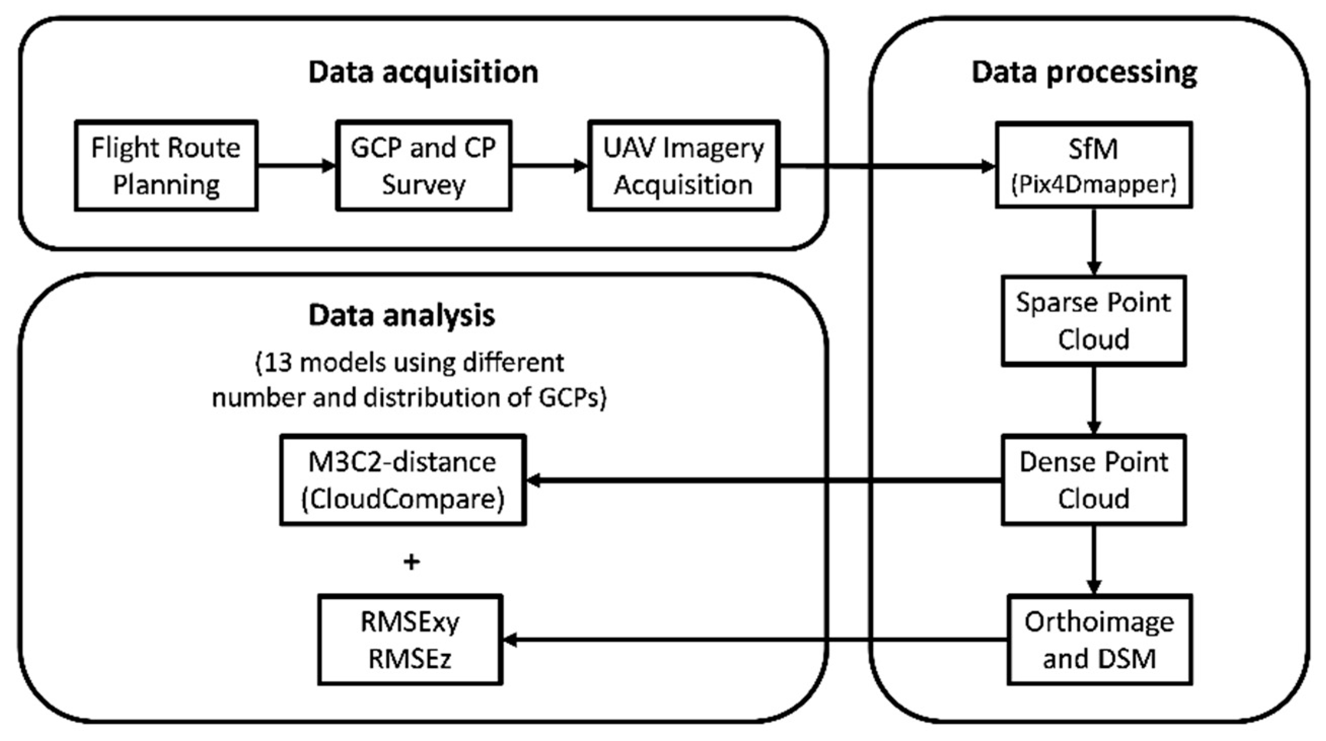
2. Materials and Methods

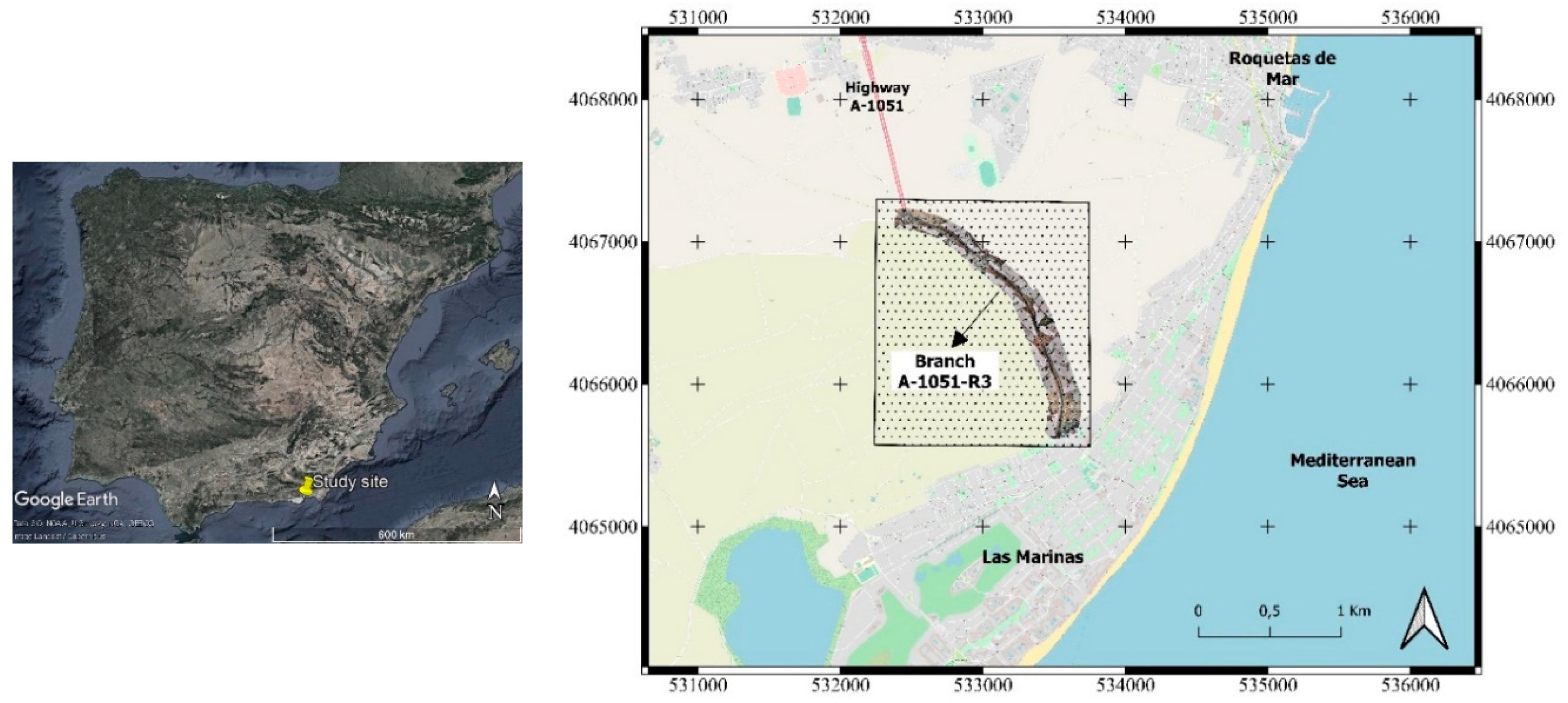
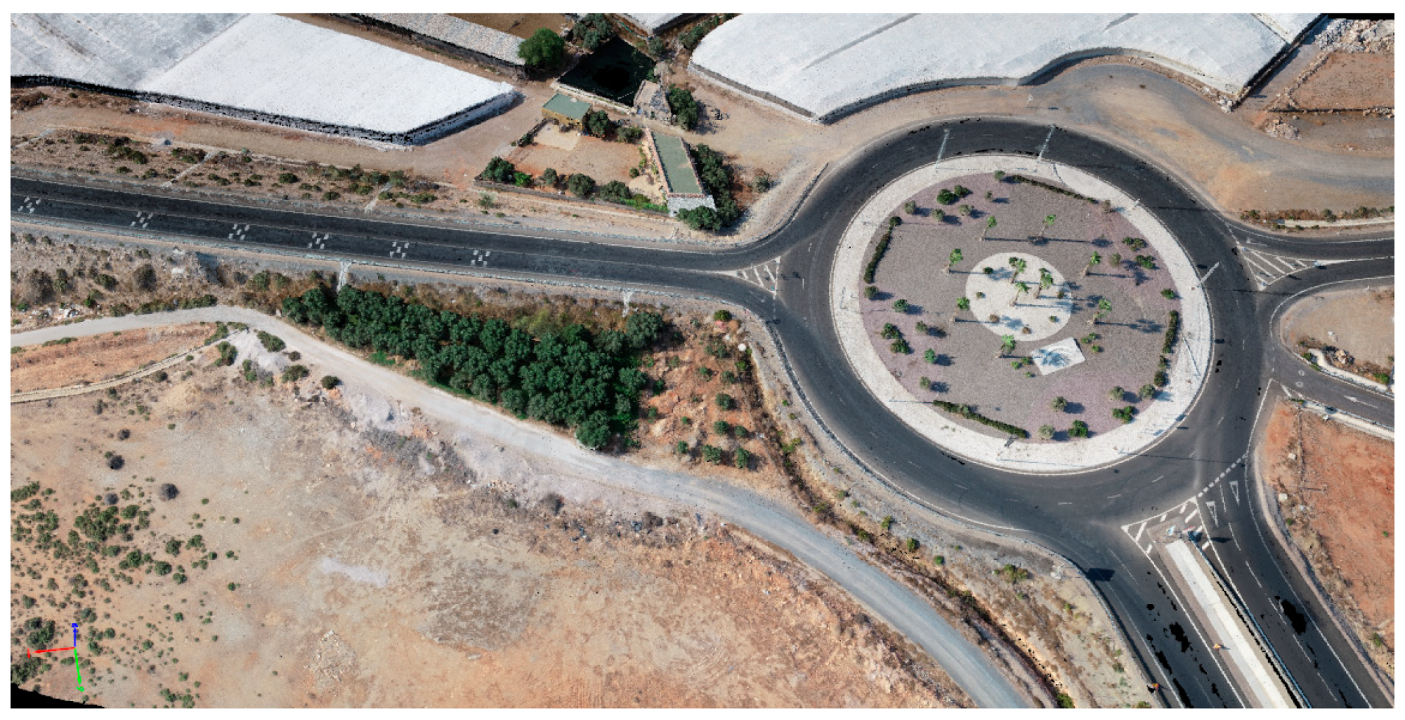
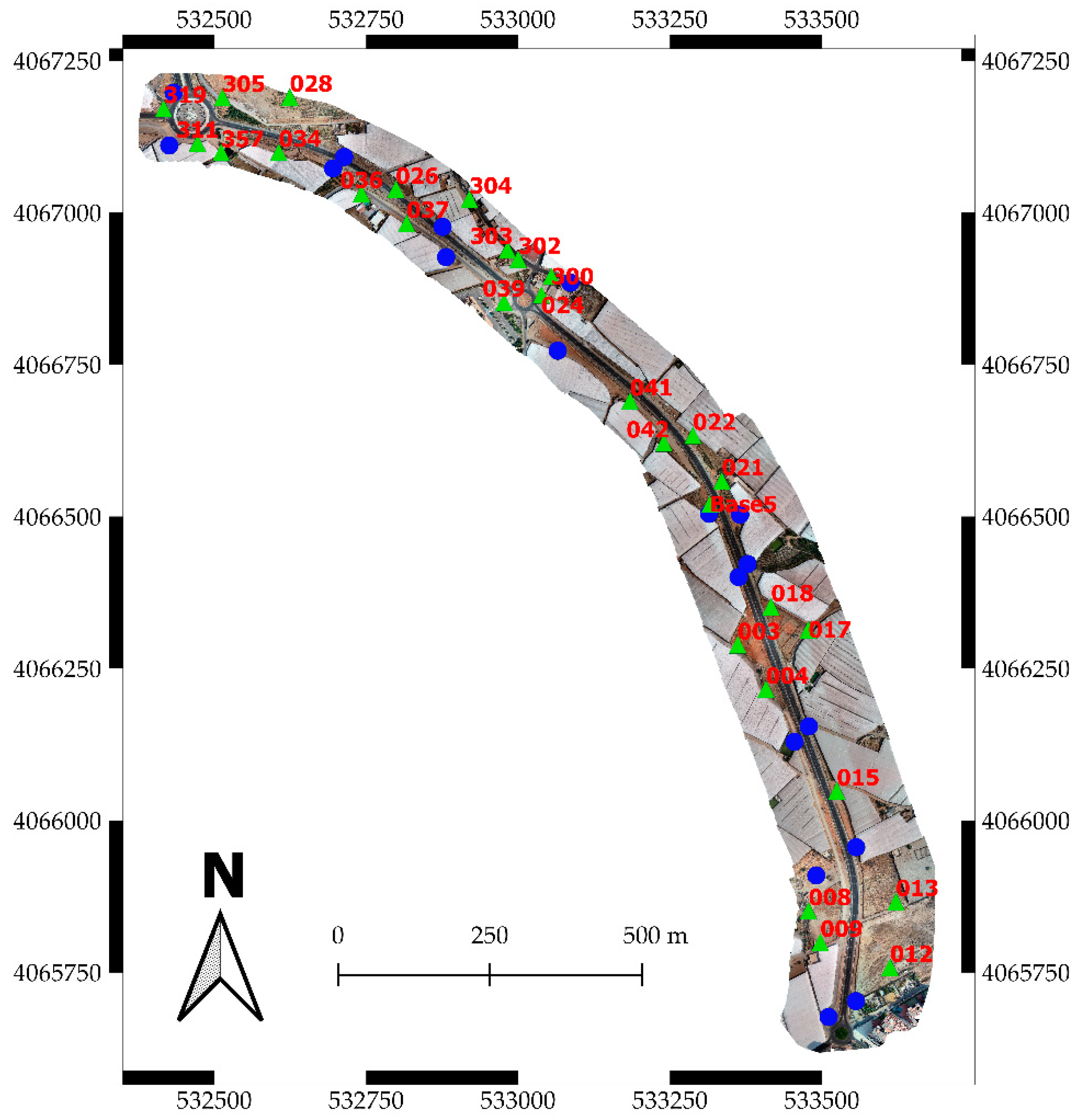
The methodology used to assess the accuracy of the different photogrammetric projects carried out is summarized in Figure 1.

2.1. Study Site

All coordinates of this study are given in meters and refer to UTM Zone 30N (European Terrestrial Reference System 1989, ETRS89) and the EGM08 geoid model. The study area is located in Roquetas de Mar (Almería), southeast Spain (Figure 2). The southwest and northeast coordinates are 533682, 4065630 and 532371, 4067232, respectively. The study site covers the A-1051-R3 branch road from the A-1051 highway, which measures 2.1 km × 190 m, with 95 m on each side of the road axis, and covers an area of approximately 40 ha. The main feature of the study site is that, in planimetry, one dimension is much larger than the other. The elevation in the studied area varies from 7 to 38 m above mean sea level. Figure 3 shows 3D cloud points corresponding to the northern end of the study site, showing a roundabout and several greenhouses, used for growing horticultural crops.

2.2. Data Acquisition

The images used in this study were taken from a rotary wing UAV with four motors. The model employed was the DJI Phantom 4 Pro, which integrates a camera equipped with a one inch and 20 megapixel CMOS sensor, and a f2.8–/f11 wide-angle lens with an equivalent focal length of 24 mm [36].

The whole study area was covered by four different flights, each covering approximately 525 m of the road. Each flight was autonomous, meaning that the UAV followed a previously programmed and loaded path consisting of two passes parallel to the road axis. The flight speed was set at 3 m s⁻¹ with images being taken every three seconds in order to achieve an 80% forward overlap. The side overlap was fixed at 60%. The flight altitude was constant at 65 m above ground level, implying that every photo covered a surface of 85.12 × 63.84 m². This resulted in an equivalent ground sample distance (GSD) of 1.75 cm pixel⁻¹. A total of 746 images were selected from the four flights to use in the photogrammetric projects.

Prior to the UAV flight, 47 targets were evenly arranged across the study area (Figure 4) to be used as GCPs or CPs. While GCPs help to georeference the project by establishing the coordinates of the model, CPs are used to assess its accuracy. Since the shape of the models adapts to the GCPs, independent CPs are used to assess accuracy by avoiding possible overestimations [25]. These points were surveyed using rover and base GPS receivers, model Trimble R6, working in post-processed kinematic (PPK) mode, and locating the base station within the range of 1 km away to all the measured points. The base station coordinates were previously determined from the geodesic pillar Las Lomas through a fast static process. The base station’s 3D coordinates are 533315.482, 4066520.639, and 24.370 m, respectively. For the PPK measurements, according to the manufacturer’s specifications, an error of 8 mm + 1 ppm RMS horizontal and 15 mm + 1 ppm RMS vertical can be expected [37].

2.3. Image Processing

The photogrammetric process was carried out using an algorithm based on SfM-MVS techniques. The workflow consists of a three-step process. In the first step, the algorithm searches for common points, usually known as key points, among the uploaded images in order to align them through a matching process. When two different key points from two different images are identical, they become matching points. These matching points, as well as the approximate values of the image position automatically extracted from the EXIF metadata, allow the algorithm to carry out a bundle adjustment and calculate the 3D coordinates of each point. To improve the geolocalization accuracy, the process was supported by both the loading of the GCP coordinates, measured as indicated in the previous section, and the marking of these GCPs in the images. The results obtained from this first step are the exact camera position and orientation for every image, the internal camera calibration parameters, and the 3D coordinates of the sparse point cloud referred to the local coordinated system selected. In the second step, the sparse point cloud is densified through the MVS technique. This technique uses the calculated camera parameters to obtain a higher point cloud density and therefore a more detailed 3D model. The 3D textured mesh is also generated during this second step. In the third step, the DSM can be generated from the densified point cloud, and, in turn, the georeferenced orthomosaic is generated using the DSM. This entire process was carried out by the commercial UAV processing software Pix4Dmapper, version 4.5.6 [38].

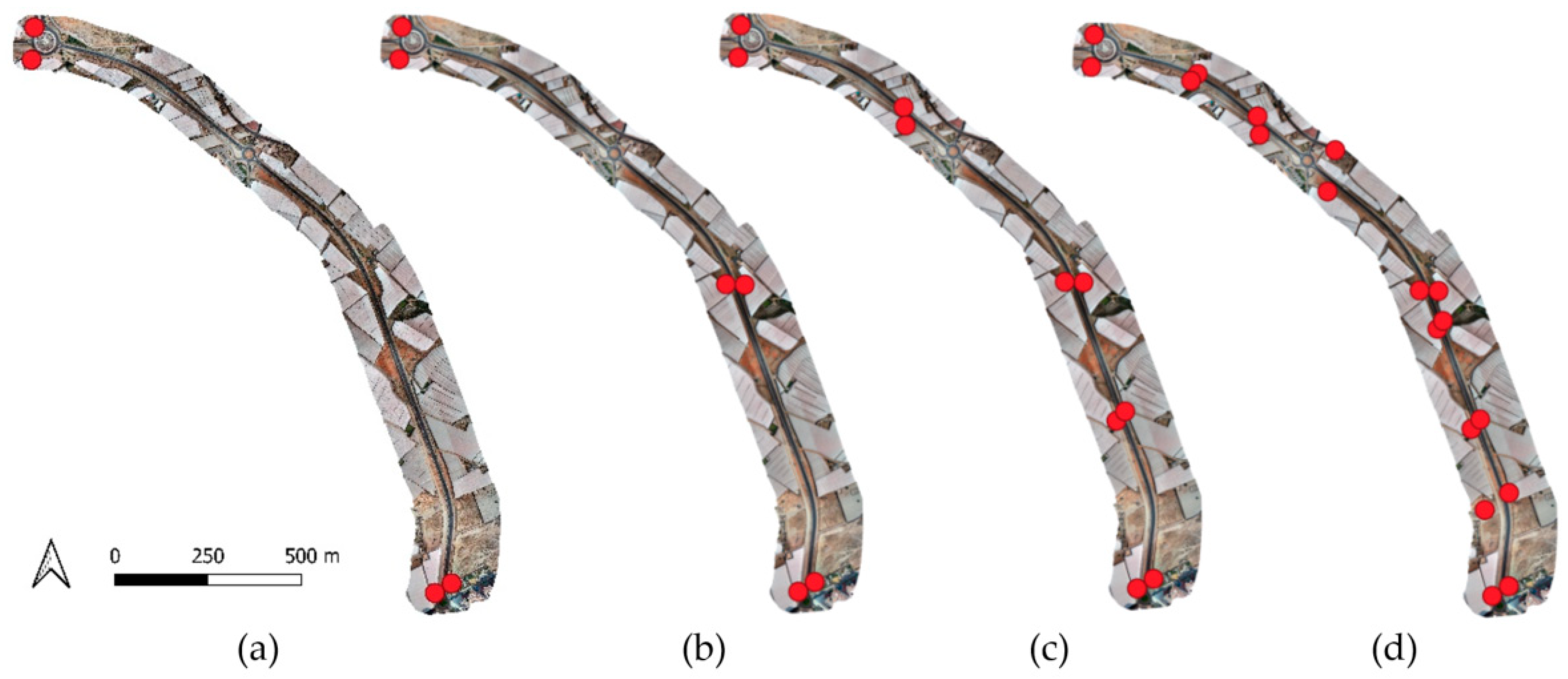
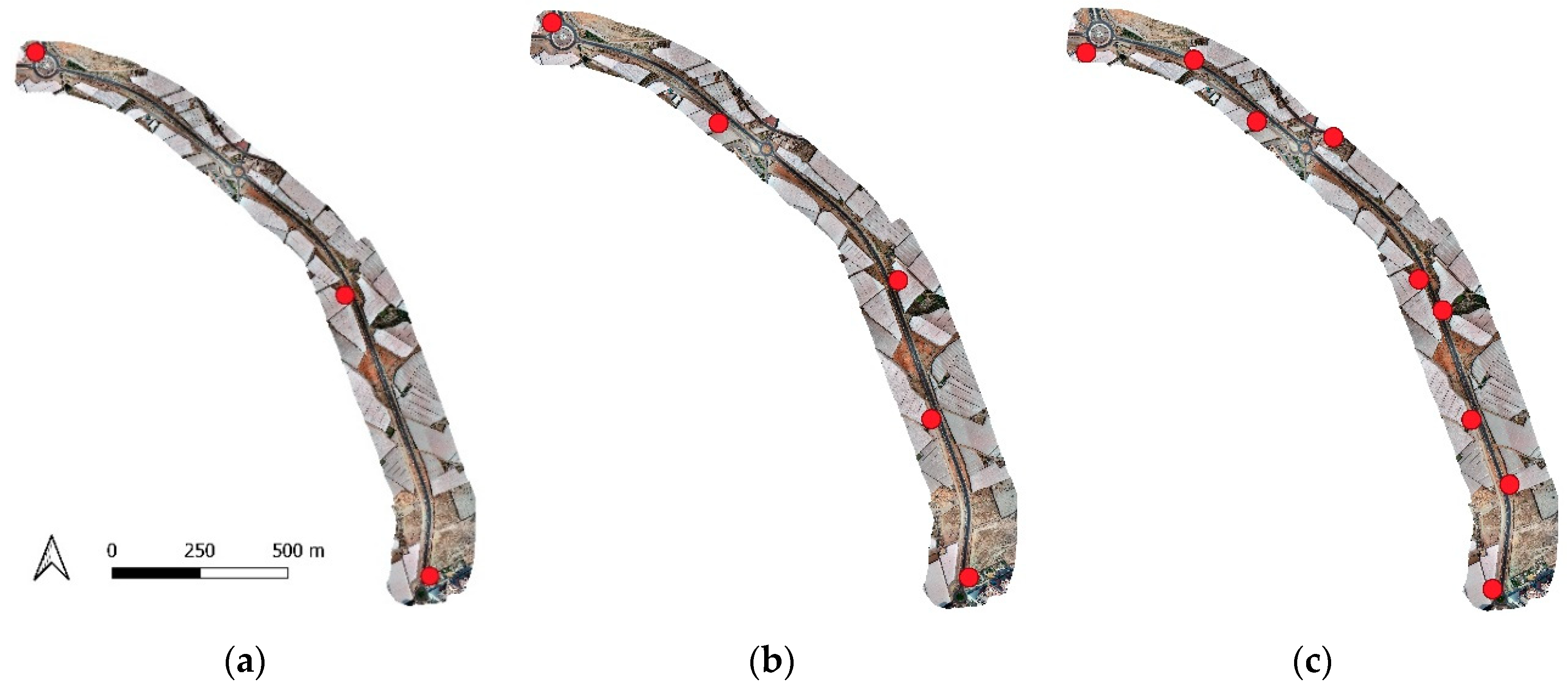
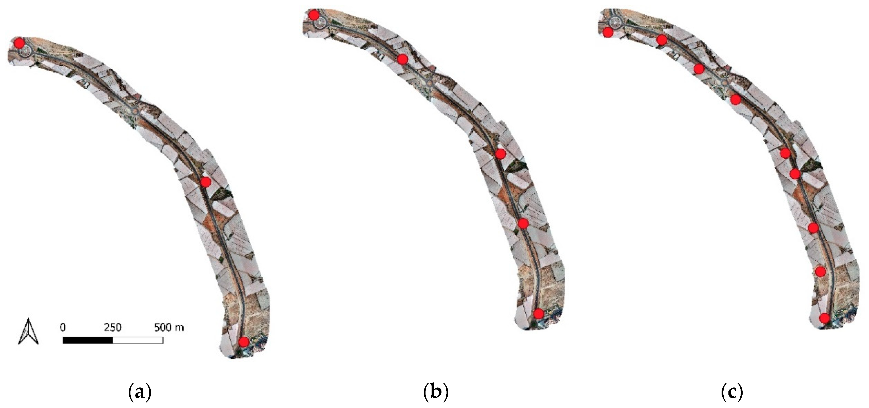
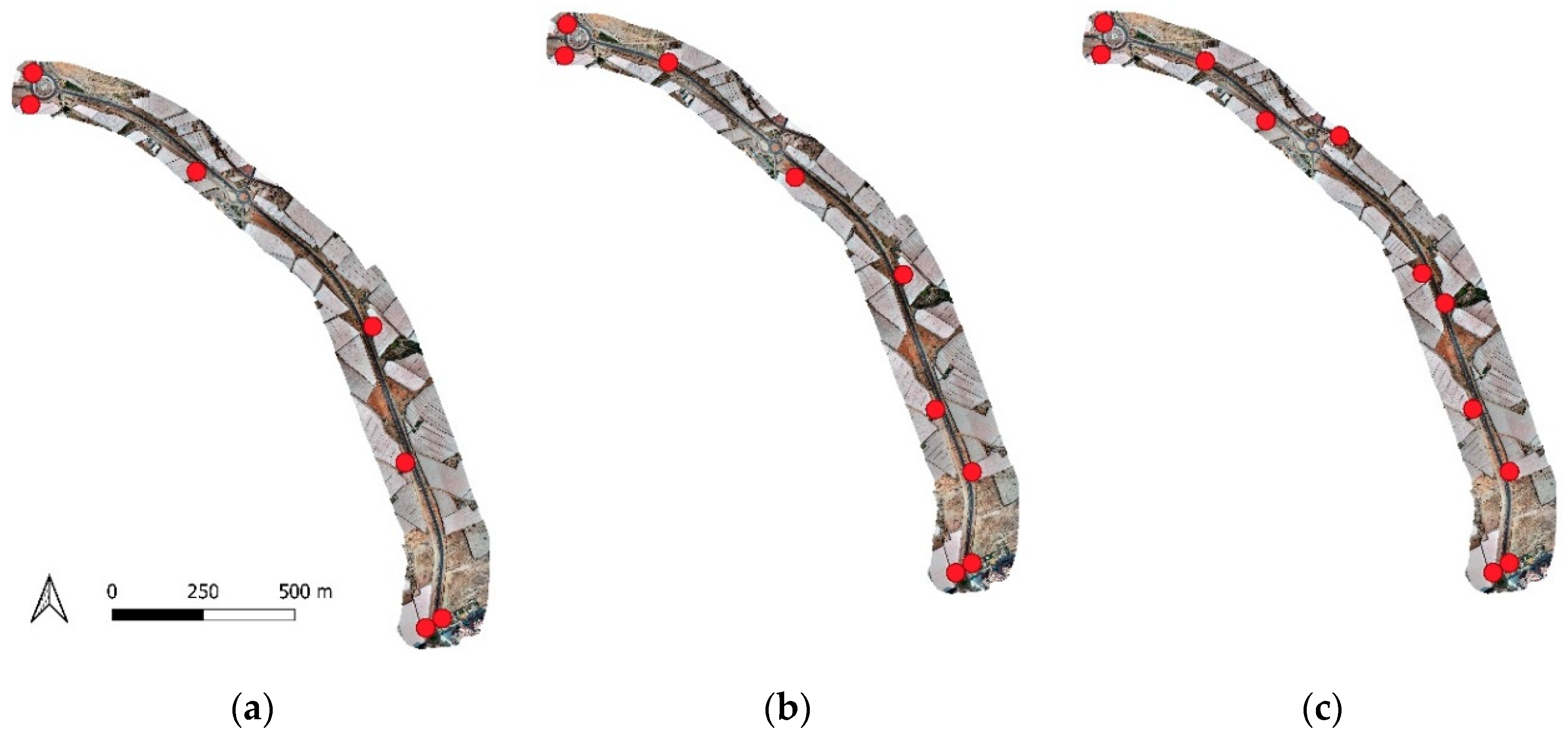
2.4. Ground Control Points

Of the 47 targets placed on the ground of the study site, 18 were used as GCPs, while the remaining 29 were used as CPs.

To assess the influence of the number of GCPs and their distribution on the accuracy of the photogrammetric linear projects, 13 different configurations were designed. For this purpose, four GCP distributions, with projects using different numbers of GCPs within each type of distribution, were taken into account for the bundle adjustment. The number of CPs employed for all projects remained constant, independently of the number of GCPs used. The different distributions studied were:

Distribution 1:

GCPs were located on both sides of the road and faced each other, as indicated by the red dots in Figure 5. Within this distribution, four projects using 4, 6, 10, and 18 GCPs were performed (Figure 5a–d). The pairs of GCPs were chosen so that they were similarly spaced from one another.

Distribution 2:

GCPs were located on both sides of the road in an offset or zigzagging pattern, as indicated by the red dots in Figure 6. For this configuration, three different projects were carried out using three, five, and nine GCPs (Figure 6a–c).

Distribution 3:

GCPs were located on only one side of the road, as indicated by the red dots in Figure 7. Under this distribution, three different projects employing three, five, and nine GCPs were developed (Figure 7a–c).

Distribution 4:

as in Distribution 2, GCPs were located on both sides of the road in a zigzagging pattern, but there was an additional pair of GCPs located at each end of the corridor. Under this distribution, three projects were carried out using 7, 9, and 11 GCPs (Figure 8a–c). This configuration can be considered as a combination of Distributions 1 and 2.

2.5. Accuracy Assessment

Two different methods are used to assess the accuracy of photogrammetric products. The first method is the mean square root of square differences between the reconstructed model and the surveyed coordinates of the 29 CPs, known as root mean square error (RMSE), since it can compensate errors with positive and negative values [39]. Differences between the reconstructed model and the surveyed coordinates are called errors, and the effect of each error on the RMSE of each error is proportional to the size of the squared error. Thus, RMSE is sensitive to estimated outlier values because large errors have a big effect on RMSE. Therefore, it is advisable to study the value of the error for each CP to check whether it is an outlier and, if so, to try to find the cause.

The RMSE values for the X component, Y component, XY component, and Z component are estimated as shown in Equations (1)–(4).

$${\mathrm{RMSE}}_{\mathrm{X}}=\sqrt{\frac{{\sum }_{\mathrm{i}=1}^{\mathrm{n}}{({\mathrm{X}}_{\mathrm{Oi}}{-\mathrm{X}}_{\mathrm{GPSi}})}^2}{\mathrm{n}}}$$

(1)

$${\mathrm{RMSE}}_{\mathrm{Y}}=\sqrt{\frac{{\sum }_{\mathrm{i}=1}^{\mathrm{n}}{({\mathrm{Y}}_{\mathrm{Oi}}{-\mathrm{Y}}_{\mathrm{GPSi}})}^2}{\mathrm{n}}}$$

(2)

$${\mathrm{RMSE}}_{\mathrm{XY}}=\sqrt{\frac{{\sum }_{\mathrm{i}=1}^{\mathrm{n}}{[{({\mathrm{X}}_{\mathrm{Oi}}{-\mathrm{X}}_{\mathrm{GPSi}})}^2+({\mathrm{Y}}_{\mathrm{Oi}}{-\mathrm{Y}}_{\mathrm{GPSi}}\left)\right]}^2}{\mathrm{n}}}$$

(3)

$${\mathrm{RMSE}}_{\mathrm{Z}}=\sqrt{\frac{{\sum }_{\mathrm{i}=1}^{\mathrm{n}}{({\mathrm{Z}}_{\mathrm{Oi}}{-\mathrm{Z}}_{\mathrm{GPSi}})}^2}{\mathrm{n}}}.$$

(4)

where:

n is the number of CPs;

X_Oi, Y_Oi, and Z_Oi are the X, Y, and Z coordinates estimated by the model for the i^th CP, respectively;

X_GPSi, Y_GPSi, and Z_GPSi are the X, Y, and Z coordinates measured by GPS for the i^th CP, respectively. The second method used in this study to assess the accuracy of the point clouds obtained through a UAV paired with SfM-MVS techniques consists of the freely available Multiscale Model to Model Cloud Comparison (M3C2) plugin offered by the CloudCompare software [40]. For the comparison of the different point clouds, a reference cloud was computed using the 47 surveyed points as GCPs, assuming that it is the most accurate and precise that can be achieved with the available data.

The M3C2 algorithm calculates the local differences between the reference cloud and the compared point cloud relative to local surface normal orientation. The algorithm does this through two different steps [41]:

• A user-defined diameter of the spherical neighborhood in the reference point cloud is used to compute the local normal orientations. This user-defined diameter is known as the normal scale;
• The normal orientation calculated is then used to project a cylinder, with a user-defined diameter called the projection scale, inside which equivalent points in the compared point cloud are searched for. From the points intercepted within the cylinder in each cloud, the average position along the normal direction is calculated for both clouds. The local distance between the two clouds is then given based on the distance between these averaged positions.

To ensure that the normal orientation is unaffected by point cloud roughness, the normal scale was set as 25 times the average local roughness calculated for the reference point cloud by CloudCompare [41]. To compare point clouds, the M3C2 distances between the reference point cloud and the point clouds generated for the 13 projects were calculated. Mean and standard deviation values calculated from the M3C2 distance were then used to assess the accuracy and the precision, respectively, of each point cloud. The mapping of the errors and their distribution curve allowed us to determine the influence of the GCP distribution on the M3C2 difference spatial distribution and to identify possible patterns for the spatial distribution of the errors.

3. Results

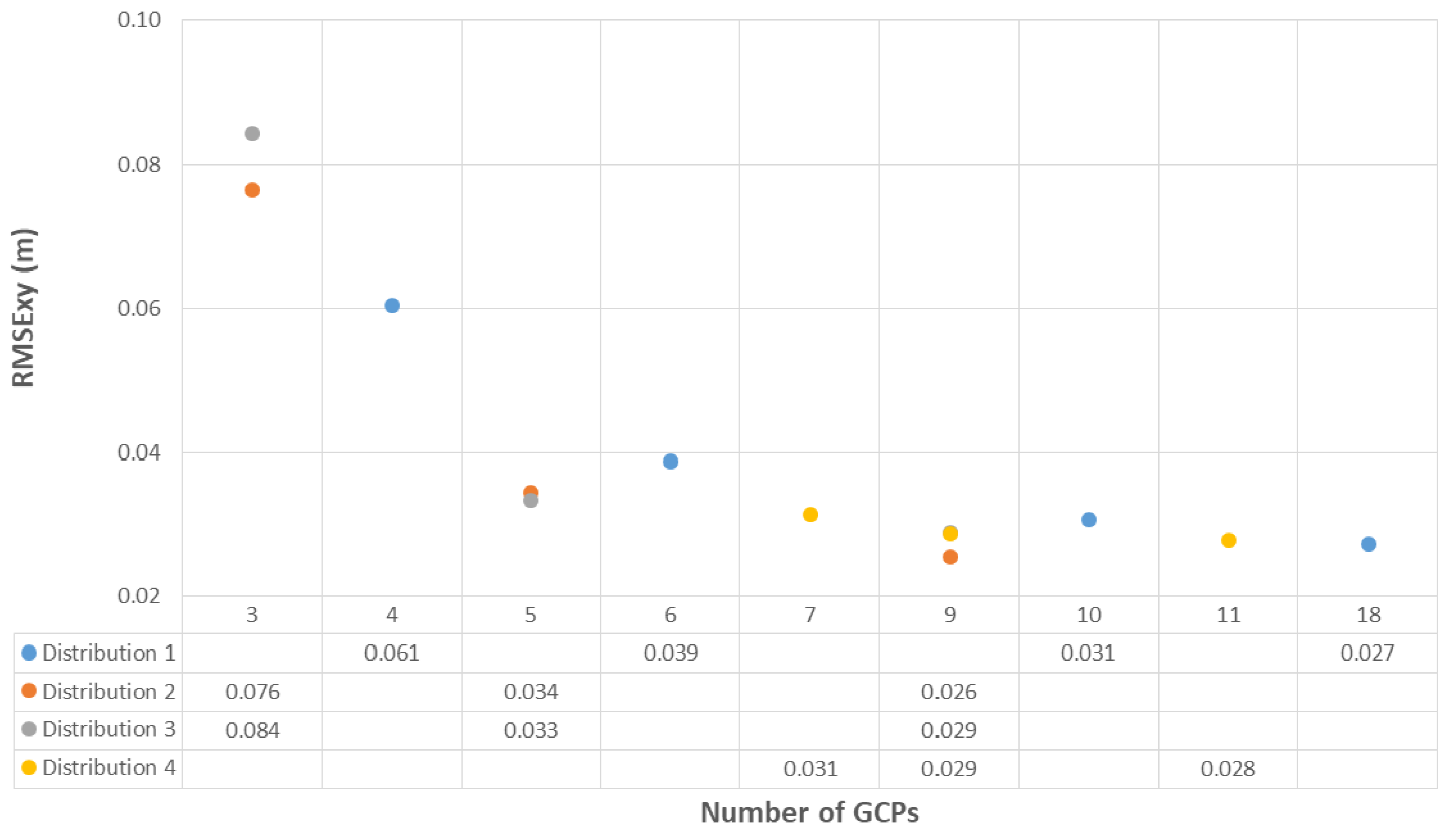
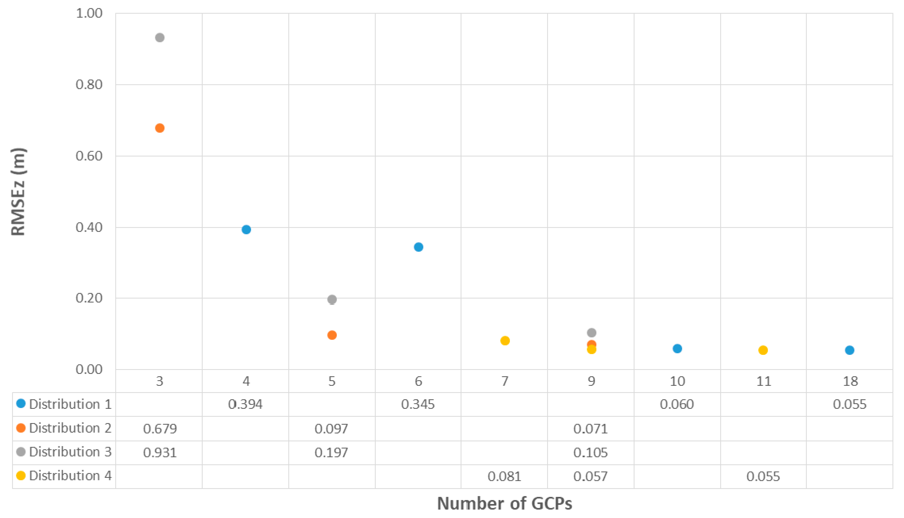
3.1. Accuracy Based on RMSE

For all four types of distribution considered in this study, the planimetric accuracy (RMSE_XY) decreases as the number of GCPs increases (Figure 9). For Distribution 1, in which GCPs were placed on both sides of the road facing each other, RMSE_XY values ranged from 0.061 using 4 GCPs to 0.027 m using 18 GCPs. For Distribution 2, in which GCPs were located on both sides of the road and offset from one another, RMSE_XY values ranged from 0.076 using three GCPs to 0.026 m using nine GCPs. For Distribution 3, in which GCPs were located on only one side of the road, RMSE_XY ranged from 0.084 using three GCPs to 0.029 m using nine GCPs. Finally, for Distribution 4, in which GCPs were placed according to a combination of Distributions 1 and 2, the planimetric error ranged from 0.031 using 7 GCPs to 0.028 m using 11 GCPs. Our results show that an increase in the number of GCPs used in the bundle adjustment leads to an increase in planimetric accuracy, independent of the spatial distribution. Only five GCPs (approximately 2.4 GCPs km⁻¹) were necessary to achieve an RMSE_XY less than two times the GSD of the project, and no fewer than nine GCPs (4.3 GCPs km⁻¹) were required to achieve RMSE_XY values less than 0.03 m. The improvement in planimetric accuracy when 18 GCPs (8.6 GCPs km⁻¹) were used was less than 0.01 m compared to the accuracy obtained with five GCPs. The increase in accuracy became insignificant when more than nine GCPs were used.

Our results also show that GCP distribution influences planimetric accuracy. Distributions 2 and 3 yielded very similar results. Furthermore, with an identical number of GCPs, Distributions 2 and 3 achieved better accuracy values than Distribution 1. Distribution 4 also improves upon the results obtained by Distribution 1, yielding better or similar accuracy values with fewer GCPs. The lowest RMSExy value was obtained with nine GCPs in a Distribution 2 configuration.

For all the photogrammetric projects performed, the values obtained for vertical accuracy (RMSE_z) are higher than those obtained for RMSE_xy. As with planimetric accuracy, the RMSE_z also decreases as the number of GCPs used for the bundle adjustment increases for the four types of distribution (Figure 10). RMSE_z values ranged from 0.394 to 0.055 m for Distribution 1, from 0.679 to 0.071 m for Distribution 2, from 0.931 to 0.105 m for Distribution 3, and from 0.081 to 0.055 m for Distribution 4.

Independent of the distribution, at least seven GCPs (3.3 GCPs km⁻¹) are necessary to achieve RMSE_z values significantly less than 0.1 m, and nine or more are required to obtain values less than 0.06 m. Three projects were close to the recommended RMSE_z value of three times the GSD of the project (0.053 m) [35]. For all distributions, the accuracy improves along with the number of GCPs included. For Distribution 1, the difference between the use of 10 and 18 GCPs is less significant considering the large increase in the number of GCPs. The accuracies obtained for projects in Distribution 1 using 10 and 18 GCPs and in Distribution 4 using 9 and 11 GCPs are very similar, ranging from 0.055 to 0.06 m.

Regarding vertical accuracy, the influence of GCP distribution is more evident than for planimetric accuracy. While Distributions 2 and 3 yielded similar results in terms of horizontal accuracy, when it comes to height accuracy, Distribution 2 achieves lower RMSE_z values, with a difference of up to 0.03 m when nine GCPs are used.

Distribution 1 significantly improves the vertical accuracy obtained for Distributions 2 and 3. Using just 11 GCPs, Distribution 4 achieves an RMSE_z value similar to the accuracy yielded with 18 GCPs in Distribution 1 (0.055 m). Furthermore, with the use of nine GCPs in Distribution 4, a very close value (0.057 m) to Distribution 1 with 18 GCPs (0.055m) was obtained.

Taking into account both horizontal and vertical accuracy, the configurations with the lowest total RMSEs are Distribution 1 with 18 GCPs (8.6 GCPs km⁻¹, RMSE_XY = 0.027 m, RMSE_Z = 0.055 m), and Distribution 4 with 11 GCPs (5.2 GCPs km⁻¹, RMSE_xy = 0.028 m, RMSE_z = 0.055 m). The configuration with nine GCPs (4.3 GCPs km⁻¹) in Distribution 4 yielded a total RMSE value of 0.064 m. For the remaining configurations, the total RMSE is 0.07 m in the case of 10 GCPs (4.8 GCP km⁻¹) in Distribution 1, while the other distributions resulted in better values.

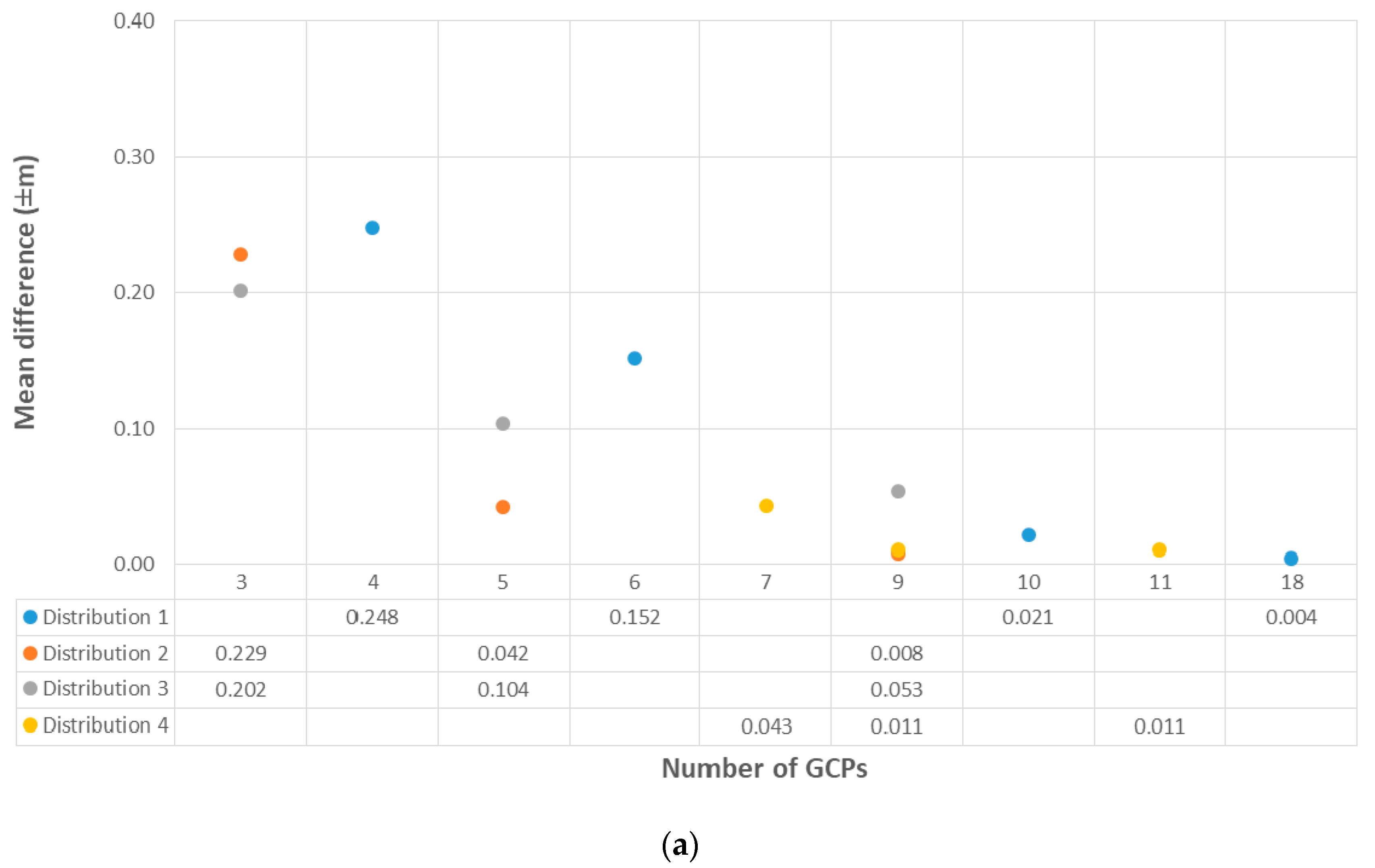
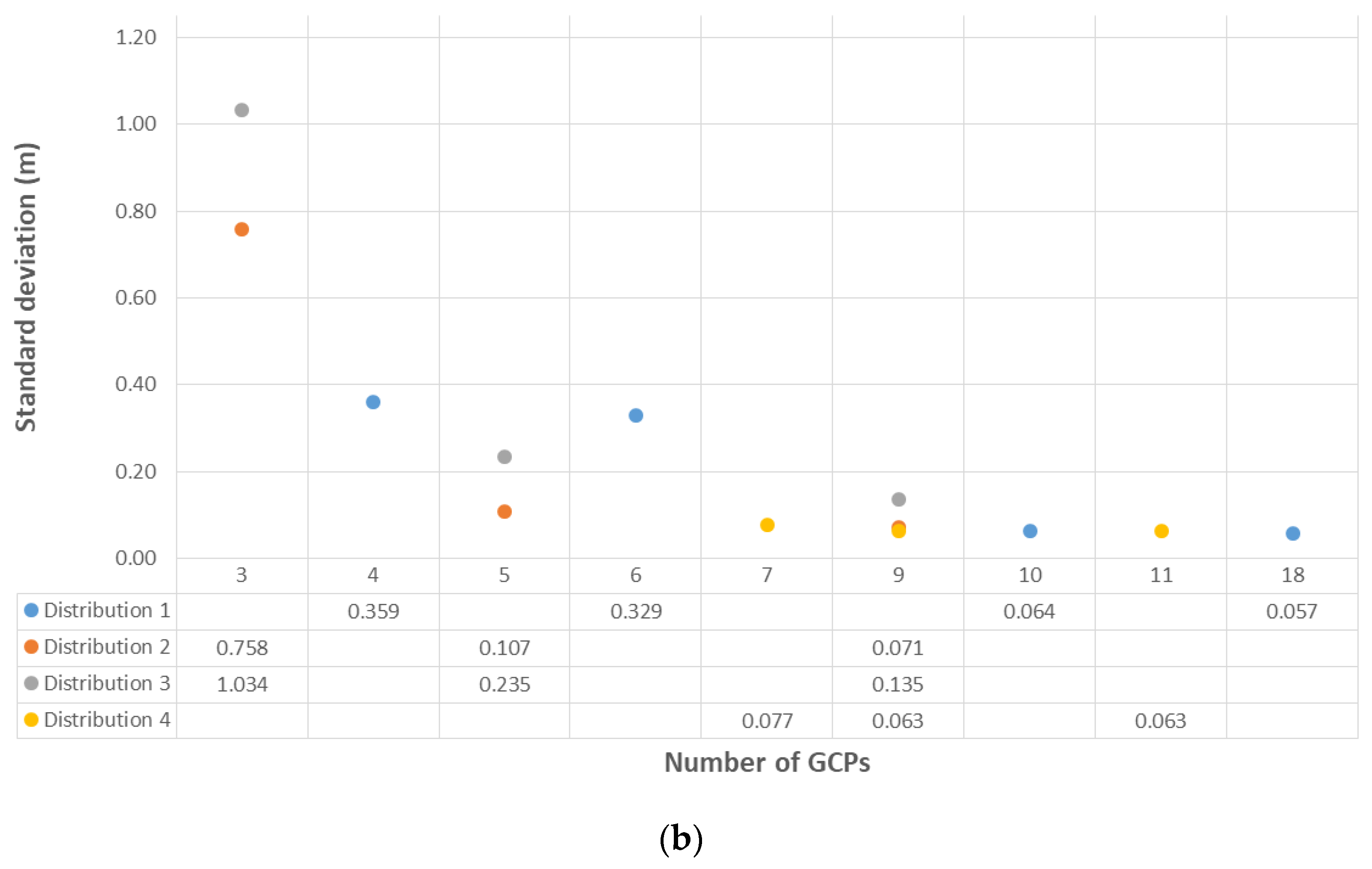
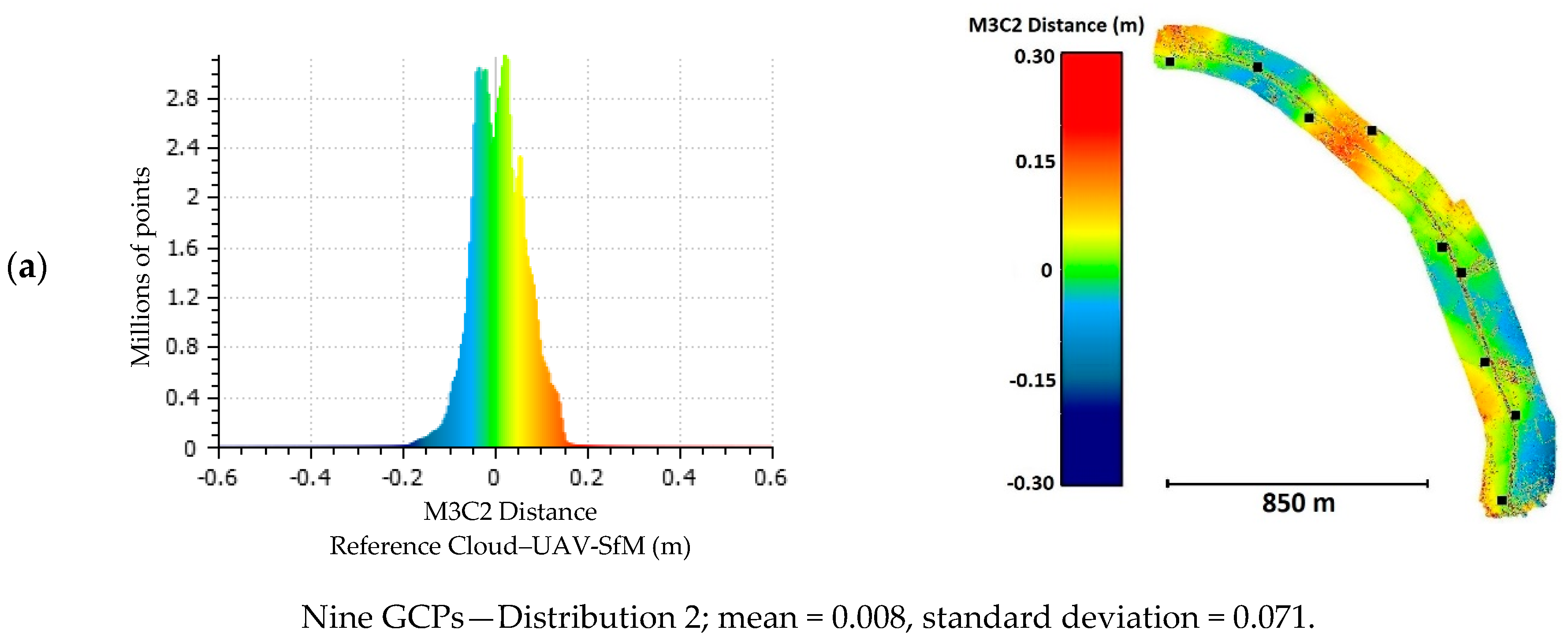
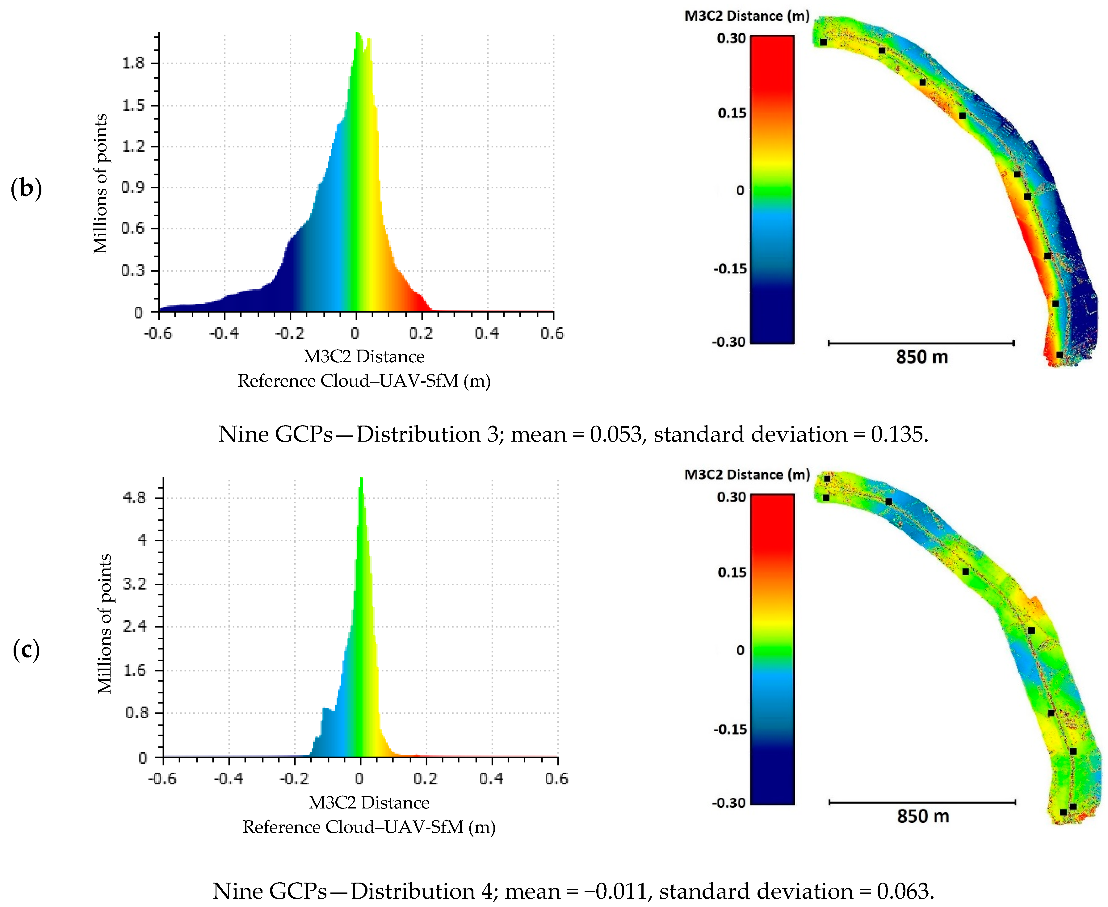
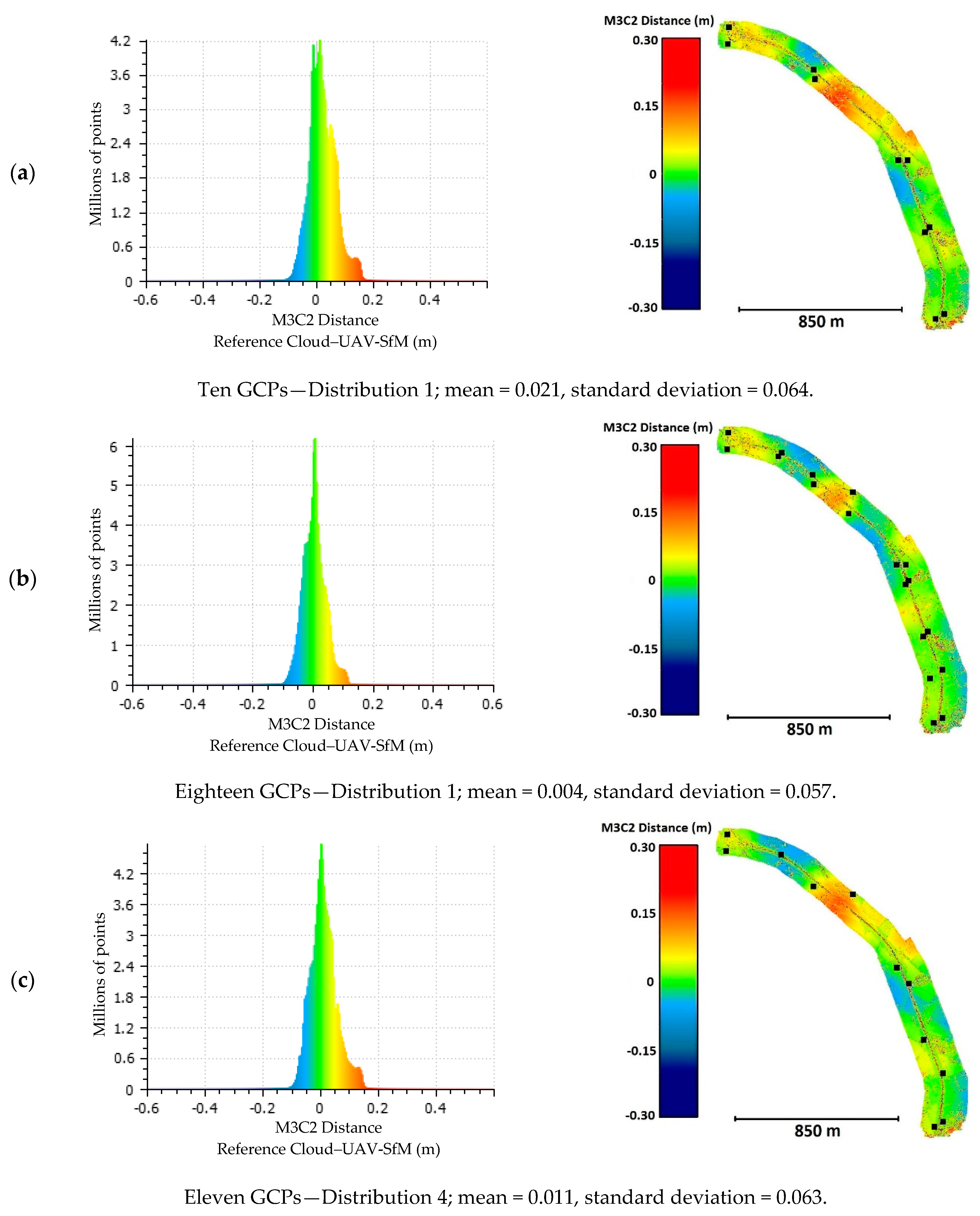
3.2. Accuracy Based on M3C2-Distances

For every distribution, point clouds become more accurate and more precise as the number of GCPs increases. In most cases, with nine GCPs or more, mean difference values are around 0.02 m or less and standard deviation values are less than 0.07 m. Distribution 3 yielded the worst results with nine GCPs: 0.053 m (Figure 11).

Further, for the majority of the projects carried out, neither accurate nor precise point clouds were achieved with fewer than seven GCPs, regardless of the type of distribution employed. Distribution 3 presents higher standard deviations and mean values, which means lower precision and accuracy than the other distributions. For projects with nine GCPs, the one placed according to Distribution 2, yielded better accuracy but lower precision than those with 9 and 11 GCPs in Distribution 4. Distribution 1 with 18 GCPs resulted in the lowest standard deviation and smallest mean difference than any other configuration, although similar values can be achieved with 9 or 11 GCPs placed according to Distribution 4.

In order to better understand how the distribution of GCPs impacts the accuracy of the projects, the spatial distributions of the M3C2-calculated distance between the reference cloud and the clouds from the photogrammetric projects were analyzed. For this purpose, only projects that used nine or more GCPs were considered (Figure 12 and Figure 13).

Although the mean difference was lower for Distribution 2, the precision improved considerably when a pair of GCPs was placed at each end of the corridor (Distribution 4, Figure 12). Distribution 2 (mean = −0.008 m, standard deviation = 0.071 m) and Distribution 4 (mean = −0.011 m, standard deviation = 0.063 m) achieved much better results for both accuracy and precision than Distribution 3, which yielded a higher mean (0.053 m) and standard deviation (0.135 m).

Figure 13 shows the spatial distributions of the M3C2-calculated distance between the reference cloud and the clouds generated from the photogrammetric projects in which more than nine GCPs were used to carry out the bundle adjustment. Although the project with 18 GCPs yielded the lowest values for both accuracy (0.004 m) and precision (0.057 m), close values can be obtained with just 9 (accuracy = −0.0121 m, precision = 0.0643 m, Figure 12) or 11 GCPs (accuracy = 0.011 m, precision = 0.063 m) placed according to Distribution 4. This distribution has better values of accuracy and precision with both 9 (accuracy = −0.011 m, precision = 0.063 m) and 11 (accuracy = 0.011 m, precision = 0.063 m) GCPs than those of Distribution 1 with 10 GCPs (accuracy = 0.021 m, precision = 0.064 m). This could be caused by the better distribution of GCPs in Distribution 4 than in Distribution 1, where the pairs of GCPs are very close.

4. Discussion

In the literature, there is little research that focuses on studying the effect of the number and distribution of GCPs on the accuracy of UAV photogrammetric projects on corridors. Most of the studies are focused on surfaces where one dimension is not much larger than the other. Skarlatos et al. [35], on a corridor measuring 2.2 km × 160 m, used a GCP distribution similar to our Distribution 4, with two points at each end of the corridor and others (one, two, and three points) along the corridor. Therefore, their project with seven GCPs is equivalent to our Distribution 4 with seven GCPs, which represents 3.3 GCPs km⁻¹. In this situation, Skarlatos et al. reported an RMSE_xy = 0.130 m and an RMSE_z = 0.170 m, while our results were RMSE_xy = 0.031 m and RMSE_Z = 0.081 m. The main difference between Skarlatos et al.’s study and our own is the GSD: 0.040 m for their images and 0.0175 m for our images. If we consider the GSD, Skarlatos et al. achieved horizontal and vertical accuracies of approximately three and four times the GSD. In our work, the planimetric accuracy was better (less than two times the GSD of the project), but the vertical was similar (in the range of four times the GSD). These accuracies can be improved by adding more GCPs, independently of their distribution. When Skarlatos et al. used all 16 measured points as GCPs, they report an RMSE_xy = 0.070 m and an RMSE_z = 0.130 m, which are higher than those found in our work for Distribution 4 with 11 GCPs (RMSE_xy = 0.028 m and a RMSE_z = 0.055 m). If we again consider using the GSD to compare the results, the values are similar: 1.75 and 1.6 GSD for horizontal accuracy and 3.25 and 3.14 GSD for vertical accuracy. In any case, it should be noted that the accuracy values of Skarlatos et al. when 16 GCPs were considered were calculated from the GCPs themselves.

Tahar [22] evaluated different numbers of GCPs in a UAV photogrammetric block. Although Tahar did not indicate the linear dimension of the study area, the text refers a road to this. Several combinations of numbers (from four to nine) and distributions of GCPs were tested to study their influence on the achieved accuracy. The best RMSEs calculated in that study were reached using nine GCPs: 0.48 m for the horizontal component, and 0.78 m for the vertical component, which are larger than any value found in any of our projects. In that work, the GSD is not reported, so it is not possible to make a comparison using this value.

Zulkipli and Tahar [9] focused on using UAV as a tool to capture data of the ground for road design. Considering that the study site was not a corridor and the results are not comparable to ours, they obtained RMSE values of 0.155, 0.228, and 0.479 m for X, Y, and Z, respectively, with six GCPs and a fly height of 148 m (the GSD value is not reported). These values mean that, although the height accuracy is close to the one presented in the present study for six GCPs and Distribution 1, the planimetric accuracy is much higher for the same number of GCPs since an increase in the number of GCPs is necessary to improve the accuracy of photogrammetric projects, as the authors concluded. Nevertheless, since the fly height of the present study is 65 m, while in Zulkipli and Tahar it was 148 m, their GSD was likely larger than ours, and it is important to note that, as the flight height (and, in turn, the GSD) increases, the accuracy deteriorates [27]. One of our main findings is that the project using more GCPs was not the most accurate. It is very important to consider not only the number of GCPs but also their distribution across the study area.

Tournadre et al. [34] aimed to present a method to assure precise accuracy in UAV photogrammetric projects of linear works and to minimize the number of GCPs required. Their study was developed on a corridor of 600 × 15 m. The influence of camera calibration, the inclusion of oblique images, and the number of GCPs on the magnitude of the bowl effect in the UAV photogrammetric project was studied. They concluded that one GCP for each 100 m (six GCPs in the studied corridor) is the optimal distribution to reduce most of the CPs reprojection errors to less than one centimeter, they do not mention GCP distribution. Our accuracies with six GCPs are better than the accuracy given by Tournadre et al., but they do not report the project GSD.

Several studies have already proven that the distribution of the GCPs affects the accuracy of the projects, and a good geometrical distribution of GCPs will lead to better accuracies [21,29]. In terms of the distribution of GCPs, since the results of the projects using GCPs on only one side of the road were the worst in both the RMSE and M3C2 distance values, we found that, to improve the accuracy in corridor-shaped projects, it is necessary to place GCPs on both sides of the road. The distribution in which the GCPs are placed alternately on each side of the road and separated by an offset distance presented results similar to those of the distribution in which GCPs are set out in pairs along the road. However, the best results were yielded by a combination of both, in which the GCPs were set out in an offset pattern but with the addition of a pair of GCPs at each end of the road, yielding better results with just 11 GCPs (5.2 GCPs km⁻¹) than another distribution using 18 GCPs (8.6 GCPs km⁻¹). This configuration yielded values less than two and three times the GSD of the project for both horizontal and vertical accuracy.

In view of Figure 12 and Figure 13, it can be deduced that there are no significant errors in the clouds of the projects represented and that these are not concentrated in certain areas. An exception is Distribution 3 with nine GCPs (Figure 12), where values of approximately 0.3 m are reached in the southeast area. This is related to the RMSE values found for the CPs located in the same area (points 12, 13, and 17, Figure 4). In the other representations of the error distribution in Figure 12 and Figure 13, the values of the errors observed in an area are in agreement with the RMSE values calculated for the CPs located in that same area.

The results derived from both methodologies used to assess the accuracy are coherent. Similar results were obtained through these two different approaches, thus strengthening the conclusions of the work carried out. Furthermore, when the distribution of errors for the M3C2-calculated distance between the reference cloud and the clouds was obtained from the different photogrammetric projects, no bowl effect was observed, even when the number of GCPs was small.

5. Conclusions

This study was performed to assess how the number of GCPs and their distribution impact the accuracy of UAV photogrammetry projects in a corridor-shaped study site. For that purpose, several projects with different configurations were carried out on a 2.1 km road, where 47 points were surveyed to be used either as GCPs or CPs. To assess accuracy, RMSE values from the georeferencing process and the M3C2 distance from the point clouds comparison were used.

For all the distributions studied, both horizontal and vertical accuracy improved as the number of GCPs used in the bundle adjustment increased, and planimetric accuracy was always better than vertical accuracy. Independent of the chosen distribution, no fewer than seven GCPs (3.3 GCPs km⁻¹) must be used to reach values of RMSE_xy ≤ 0.031 m and RMSE_z ≤ 0.081 m. The best results were achieved for those distributions where the GCPs were placed on both sides of the road. Placing GCPs alternatively on each side of the road and separating them by an offset distance, with a pair of GCPs placed at each end of the corridor, proved to yield the best results.

Considering the results, configurations with 9 or 11 GCPs (4.3 and 5.2 GCPs km⁻¹, respectively) placed on both sides of the road in an offset pattern, with a pair of GCPs at each end, yielded the best results in terms of balancing the accuracy and fieldwork, with RMSE mean values of 0.029 and 0.028 m for horizontal and 0.057 and 0.055 m for vertical accuracy, respectively. Similar results in terms of RMSE values (0.027 for horizontal and 0.055 m for vertical) and slightly better results in terms of M3C2 distance (mean difference and standard deviation) were achieved with 18 GCPs (8.6 GCPs km⁻¹) set out in pairs along the corridor. Since every GCP must be surveyed using high-accuracy technology, the use of 9 or 11 GCPs, with the offset distribution mentioned previously, is recommended in study areas similar to that assessed in this study, since it can significantly reduce both the fieldwork and survey duration without a loss in accuracy, compared to the use of a higher number of GCPs placed according to other distributions.

To determine if the conclusions derived from this study are generally applicable, it would be necessary to carry out related studies in corridors with different terrain morphologies.

References

1. Mancini, F.; Dubbini, M.; Gattelli, M.; Stecchi, F.; Fabbri, S.; Gabbianelli, G. Using Unmanned Aerial Vehicles (UAV) for High-Resolution Reconstruction of Topography: The Structure from Motion Approach on Coastal Environments. Remote Sens. 2013, 5, 6880–6898. [Google Scholar] [CrossRef] [Green Version]
2. Mourato, S.; Fernandez, P.; Pereira, L.; Moreira, M. Improving a DSM Obtained by Unmanned Aerial Vehicles for Flood Modelling. IOP Conf. Ser. Earth Environ. Sci. 2017, 95. [Google Scholar] [CrossRef]
3. Rodrigo-Comino, J.; Seeger, M.; Iserloh, T.; Senciales González, J.M.; Ruiz-Sinoga, J.D.; Ries, J.B. Rainfall-simulated quantification of initial soil erosion processes in sloping and poorly maintained terraced vineyards—Key issues for sustainable management systems. Sci. Total Environ. 2019, 660, 1047–1057. [Google Scholar] [CrossRef] [PubMed]
4. Campbell, S.; Simmons, R.; Rickson, J.; Waine, T.; Simms, D. Using Near-Surface Photogrammetry Assessment of Surface Roughness (NSPAS) to assess the effectiveness of erosion control treatments applied to slope forming materials from a mine site in West Africa. Geomorphology 2018, 322, 188–195. [Google Scholar] [CrossRef]
5. Gong, C.; Lei, S.; Bian, Z.; Liu, Y.; Zhang, Z.; Cheng, W. Analysis of the Development of an Erosion Gully in an Open-Pit Coal Mine Dump During a Winter Freeze-Thaw Cycle by Using Low-Cost UAVs. Remote Sens. 2019, 11, 1356. [Google Scholar] [CrossRef] [Green Version]
6. Rossi, G.; Tanteri, L.; Tofani, V.; Vannocci, P.; Moretti, S.; Casagli, N. Multitemporal UAV surveys for landslide mapping and characterization. Landslides 2018, 15, 1045–1052. [Google Scholar] [CrossRef] [Green Version]
7. Menegoni, N.; Giordan, D.; Perotti, C. Reliability and uncertainties of the analysis of an unstable rock slope performed on RPAS digital outcrop models: The case of the gallivaggio landslide (Western Alps, Italy). Remote Sens. 2020, 12, 1635. [Google Scholar] [CrossRef]
8. Fernández, T.; Pérez, J.; Cardenal, J.; Gómez, J.; Colomo, C.; Delgado, J. Analysis of Landslide Evolution Affecting Olive Groves Using UAV and Photogrammetric Techniques. Remote Sens. 2016, 8, 837. [Google Scholar] [CrossRef] [Green Version]
9. Zulkipli, M.A.; Tahar, K.N. Multirotor UAV-Based Photogrammetric Mapping for Road Design. Int. J. Opt. 2018, 2018. [Google Scholar] [CrossRef]
10. Tan, Y.; Li, Y. UAV photogrammetry-based 3D road distress detection. ISPRS Int. J. Geo-Inf. 2019, 8, 409. [Google Scholar] [CrossRef] [Green Version]
11. Tsouros, D.C.; Bibi, S.; Sarigiannidis, P.G. A review on UAV-based applications for precision agriculture. Information 2019, 10, 349. [Google Scholar] [CrossRef] [Green Version]
12. Agudo, P.; Pajas, J.; Pérez-Cabello, F.; Redón, J.; Lebrón, B. The Potential of Drones and Sensors to Enhance Detection of Archaeological Cropmarks: A Comparative Study Between Multi-Spectral and Thermal Imagery. Drones 2018, 2, 29. [Google Scholar] [CrossRef] [Green Version]
13. Westoby, M.J.; Brasington, J.; Glasser, N.F.; Hambrey, M.J.; Reynolds, J.M. ‘Structure-from-Motion’ photogrammetry: A low-cost, effective tool for geoscience applications. Geomorphology 2012, 179, 300–314. [Google Scholar] [CrossRef] [Green Version]
14. Harwin, S.; Lucieer, A. Assessing the Accuracy of Georeferenced Point Clouds Produced via Multi-View Stereopsis from Unmanned Aerial Vehicle (UAV) Imagery. Remote Sens. 2012, 4, 1573–1599. [Google Scholar] [CrossRef] [Green Version]
15. Hugenholtz, C.H.; Whitehead, K.; Brown, O.W.; Barchyn, T.E.; Moorman, B.J.; LeClair, A.; Riddell, K.; Hamilton, T. Geomorphological mapping with a small unmanned aircraft system (sUAS): Feature detection and accuracy assessment of a photogrammetrically-derived digital terrain model. Geomorphology 2013, 194, 16–24. [Google Scholar] [CrossRef] [Green Version]
16. Fonstad, M.A.; Dietrich, J.T.; Courville, B.C.; Jensen, J.L.; Carbonneau, P.E. Topographic structure from motion: A new development in photogrammetric measurement. Earth Surf. Process. Landf. 2013, 38, 421–430. [Google Scholar] [CrossRef] [Green Version]
17. Snavely, N.; Seitz, S.M.; Szeliski, R. Modeling the World from Internet Photo Collections. Int. J. Comput. Vis. 2008, 80, 189–210. [Google Scholar] [CrossRef] [Green Version]
18. Ao, T.; Liu, X.; Ren, Y.; Luo, R.; Xi, J. An Approach to Scene Matching Algorithm for UAV Autonomous Navigation. In Proceedings of the 2018 Chinese Control and Decision Conference (CCDC), Shenyang, China, 9–11 June 2018; pp. 996–1001. [Google Scholar]
19. Furukawa, Y.; Ponce, J. Accurate, Dense, and Robust Multi-View Stereopsis. IEEE Trans. Softw. Eng. 2010, 32, 1362–1376. [Google Scholar] [CrossRef]
20. Agüera-Vega, F.; Carvajal-Ramírez, F.; Martínez-Carricondo, P. Assessment of photogrammetric mapping accuracy based on variation ground control points number using unmanned aerial vehicle. Meas. J. Int. Meas. Confed. 2017, 98, 221–227. [Google Scholar] [CrossRef]
21. Martínez-Carricondo, P.; Agüera-Vega, F.; Carvajal-Ramírez, F.; Mesas-Carrascosa, F.J.; García-Ferrer, A.; Pérez-Porras, F.J. Assessment of UAV-photogrammetric mapping accuracy based on variation of ground control points. Int. J. Appl. Earth Obs. Geoinf. 2018, 72, 1–10. [Google Scholar] [CrossRef]
22. Tahar, K.N. An Evaluation on Different Number of Ground Control Points in Unmanned Aerial Vehicle Photogrammetric Block. Int. Arch. Photogramm. Remote Sens. Spat. Inf. Sci. ISPRS Arch. 2013, XL-2/W2, 27–29. [Google Scholar] [CrossRef] [Green Version]
23. Reshetyuk, Y.; Mårtensson, S.G. Generation of Highly Accurate Digital Elevation Models with Unmanned Aerial Vehicles. Photogramm. Rec. 2016, 31, 143–165. [Google Scholar] [CrossRef]
24. Li, T.; Zhang, H.; Gao, Z.; Niu, X.; El-sheimy, N. Tight Fusion of a Monocular Camera, MEMS-IMU, and Single-Frequency Multi-GNSS RTK for Precise Navigation in GNSS-Challenged Environments. Remote Sens. 2019, 11, 610. [Google Scholar] [CrossRef] [Green Version]
25. Tomaštík, J.; Mokroš, M.; Surový, P.; Grznárová, A.; Merganič, J. UAV RTK/PPK method-An optimal solution for mapping inaccessible forested areas? Remote Sens. 2019, 11, 721. [Google Scholar] [CrossRef] [Green Version]
26. Kim, J.; Song, J.; No, H.; Han, D.; Kim, D.; Park, B.; Kee, C. Accuracy improvement of DGPS for low-cost single-frequency receiver using modified Flächen Korrektur parameter correction. ISPRS Int. J. Geo-Inf. 2017, 6, 222. [Google Scholar] [CrossRef] [Green Version]
27. Forlani, G.; Dall’Asta, E.; Diotri, F.; di Cella, U.M.; Roncella, R.; Santise, M. Quality assessment of DSMs produced from UAV flights georeferenced with on-board RTK positioning. Remote Sens. 2018, 10, 311. [Google Scholar] [CrossRef] [Green Version]
28. Agüera-Vega, F.; Carvajal-Ramírez, F.; Martínez-Carricondo, P. Accuracy of digital surface models and orthophotos derived from unmanned aerial vehicle photogrammetry. J. Surv. Eng. 2017, 143, 1–10. [Google Scholar] [CrossRef]
29. Sanz-Ablanedo, E.; Chandler, J.H.; Rodríguez-Pérez, J.R.; Ordóñez, C. Accuracy of Unmanned Aerial Vehicle (UAV) and SfM photogrammetry survey as a function of the number and location of ground control points used. Remote Sens. 2018, 10, 606. [Google Scholar] [CrossRef] [Green Version]
30. Nesbit, P.R.; Hugenholtz, C.H. Enhancing UAV-SfM 3D model accuracy in high-relief landscapes by incorporating oblique images. Remote Sens. 2019, 11, 239. [Google Scholar] [CrossRef] [Green Version]
31. James, M.R.; Robson, S. Straightforward reconstruction of 3D surfaces and topography with a camera: Accuracy and geoscience application. J. Geophys. Res. Earth Surf. 2012, 117, 1–18. [Google Scholar] [CrossRef] [Green Version]
32. Jaud, M.; Passot, S.; Le Bivic, R.; Delacourt, C.; Grandjean, P.; Le Dantec, N. Assessing the accuracy of high resolution digital surface models computed by PhotoScan® and MicMac® in sub-optimal survey conditions. Remote Sens. 2016, 8, 465. [Google Scholar] [CrossRef] [Green Version]
33. James, M.R.; Robson, S. Mitigating systematic error in topographic models derived from UAV and ground-based image networks. Earth Surf. Process. Landf. 2014, 39, 1413–1420. [Google Scholar] [CrossRef] [Green Version]
34. Tournadre, V.; Pierrot-Deseilligny, M.; Faure, P.H. UAV linear photogrammetry. Int. Arch. Photogramm. Remote Sens. Spat. Inf. Sci. ISPRS Arch. 2015, 40, 327–333. [Google Scholar] [CrossRef] [Green Version]
35. Skarlatos, D.; Procopiou, E.; Stavrou, G.; Gregoriou, M. Accuracy assessment of minimum control points for UAV photography and georeferencing. First Int. Conf. Remote Sens. Geoinf. Environ. 2013, 8795, 879514. [Google Scholar] [CrossRef]
36. DJI Phantom 4 Pro. Available online: https://dl.djicdn.com/downloads/phantom_4_pro/20170719/Phantom_4_Pro_Pro_Plus_User_Manual_ES.pdf (accessed on 18 July 2020).
37. Trimble Trimble R6. Available online: http://www.orient-mediterranee.com/IMG/pdf/R8-R6-R4-5800M3_UserGuide.pdf (accessed on 18 July 2020).
38. Pix4Dmapper Pix4D. Available online: https://www.pix4d.com/product/pix4dmapper-photogrammetry-software (accessed on 18 July 2020).
39. Congalton, R.G. Thematic and Positional Accuracy Assessment of Digital Remotely Sensed Data. In Proceedings of the Seventh Annual Forest Inventory and Analysis Symposium, Portland, ME, USA, 3–6 October 2005. [Google Scholar]
40. CloudCompare v2.10.2. Available online: https://www.danielgm.net/cc/ (accessed on 18 July 2020).
41. Lague, D.; Brodu, N.; Leroux, J. Accurate 3D comparison of complex topography with terrestrial laser scanner: Application to the Rangitikei canyon (N-Z). ISPRS J. Photogramm. Remote Sens. 2013, 82, 10–26. [Google Scholar] [CrossRef] [Green Version]
Figure 1. Workflow of image acquisition and processing to assess the influence of number and distribution of ground control points (GCPs) on the accuracy of linear photogrammetric projects.
Remotesensing 12 02447 g001
Figure 2. Location of the study site. Coordinates refer to UTM Zone 30N (ETRS89, EGM08 geoid model). The map of the Iberian Peninsula was extracted from Google Earth. The background map on the right side was extracted from OpenStreetMap, and the square inset is an orthophoto of the study site.
Remotesensing 12 02447 g002
Figure 3. 3D cloud point corresponding to the northern end of the study site, showing a roundabout and several greenhouses.
Remotesensing 12 02447 g003
Figure 4. Location of the 47 targets used as GCPs (blue dots) and check points (CPs) (green triangles). The coordinates refer to UTM Zone 30N (ETRS89). The red numbers indicate the CP labels.
Remotesensing 12 02447 g004
Figure 5. Location of the targets used as GCPs (red dots) for each project within Distribution 1. Four projects using (a) 4, (b) 6, (c) 10, and (d) 18 GCPs were carried out.
Remotesensing 12 02447 g005
Figure 6. Location of the targets used as GCPs (red dots) for each project within Distribution 2. Three projects using (a) 3, (b) 5, and (c) 9 GCPs.
Remotesensing 12 02447 g006
Figure 7. Location of the targets used as GCPs for each project within Distribution 3. Three projects using (a) 3, (b) 5, and (c) 9 GCPs.
Remotesensing 12 02447 g007
Figure 8. Location of the targets used as GCPs for each project within Distribution 4. Three projects using (a) 7, (b) 9, and (c) 11 GCPs (red dots) were carried out.
Remotesensing 12 02447 g008
Figure 9. RMSExy values (in meters) obtained according to the number of GCPs used in the bundle adjustment. Each distribution is represented by a different color.
Remotesensing 12 02447 g009
Figure 10. RMSEz values in meters obtained according to the number of GCPs used in the bundle adjustment. Each distribution is represented by a different color.
Remotesensing 12 02447 g010
Figure 11. Multiscale Model to Model Cloud Comparison (M3C2) distance measurements between the reference cloud and the clouds obtained from the different photogrammetric projects carried out. (a) Mean difference (accuracy); (b) standard deviation (precision).
Remotesensing 12 02447 g011aRemotesensing 12 02447 g011b
Figure 12. Distribution of errors for the M3C2-calculated distance between the reference cloud and the clouds obtained from the photogrammetric projects that used nine GCPs. The black squares represent the locations of the GCPs. (a) Distribution 2, (b) Distribution 3, and (c) Distribution 4.
Remotesensing 12 02447 g012aRemotesensing 12 02447 g012b
Figure 13. Distribution of errors for the M3C2-calculated distance between the reference cloud and the clouds obtained from the photogrammetric projects that used more than nine GCPs. The black squares represent the locations of the GCPs. (a) Project with 10 GCPs in Distribution 1, (b) project with 18 GCPs in Distribution 1, and (c) project with 11 GCPs in Distribution 4.
Remotesensing 12 02447 g013