Automatic Mapping of Landslides by the ResU-Net


1
National Institute of Natural Hazards, Ministry of Emergency Management of China, Beijing 100085, China
2
Beijing Twenty-First Century Science and Technology Development Co. Ltd., Beijing 100096, China
3
Twenty-First Century Aerospace Technology Co., Ltd., Beijing 100096, China
4
School of Soil and Water Conservation, Beijing Forestry University, Beijing 100083, China
*
Author to whom correspondence should be addressed.
Remote Sens. 2020, 12(15), 2487; https://0-doi-org.brum.beds.ac.uk/10.3390/rs12152487
Submission received: 9 June 2020
/
Revised: 3 July 2020
/
Accepted: 30 July 2020
/
Published: 3 August 2020
(This article belongs to the Special Issue Landslide Monitoring, Susceptibility, Hazard Assessment and Prediction with Remotely Sensed Big Data)
Abstract
:Massive landslides over large regions can be triggered by heavy rainfalls or major seismic events. Mapping regional landslides quickly is important for disaster mitigation. In recent years, deep learning methods have been successfully applied in many fields, including landslide automatic identification. In this work, we proposed a deep learning approach, the ResU-Net, to map regional landslides automatically. This method and a baseline model (U-Net) were collectively tested in Tianshui city, Gansu province, where a heavy rainfall triggered more than 10,000 landslides in July 2013. All models were performed on a 3-band (near infrared, red, and green) GeoEye-1 image with a spatial resolution of 0.5 m. At such a fine spatial resolution, the study area is spatially heterogeneous. The tested study area is 128 km2, 80% of which was used to train models and the remaining 20% was used to validate accuracy of the models. This proposed ResU-Net achieved higher accuracy than the baseline U-Net model in this mountain region, where F1 improved by 0.09. Compared with the U-Net model, this proposed model (ResU-Net) performs better in discriminating landslides from bare floodplains along river valleys and unplanted terraces. By incorporating environmental information, this ResU-Net may also be applied to other landslide mapping, such as landslide susceptibility and hazard assessment.
1. Introduction
In mountainous regions, massive landslides can be induced by major earthquakes or heavy rainfalls. Recent examples include the 2008 Wenchuan earthquake [1,2,3,4], 1999 Chi-Chi earthquake, and 2009 Typhoon Morakot [5]. These landslides usually spread over hundreds of thousands of square kilometers. Fast mapping of these landslides is urgently needed for post-disaster response, while it remains a challenge to the geoscience community.
Field surveys play an important role in mapping regional landslides before remote sensing emerged. From the middle of 20th century, manual interpretation of landslides from aerial photos validated by field reconnaissance has been the most commonly used tool to map widely distributed landslides [6], though which was time- and labor-consuming. In the 2000s, very high spatial resolution satellite images became available and landslide mapping has been tried semi-automatically [7]. These methods to map regional landslides are often carried out in two ways of either pixel-based or object-based image analysis [8,9]. Pixel-based methods use different characteristics between landslide pixels and non-landslide pixels to pick out landslides. For pixel-based methods, change detection based on spectral information has been the most commonly used technique [10,11,12,13]. The difference between pre- and post-event satellite images permits to easily detect landslides. In contrast, object-based classification methods take both spectral and spatial information into account to identify landslides [14,15].
For both pixel- and object-based image analysis, machine learning (ML) methods (such as random forests, support vector machine, and logistic regression) have been extensively used to identify landslides [10,16,17]. In traditional machine learning algorithms, most efforts have been focused on producing and selecting features, most of which include spectral bands of the images, spectral derivatives (Normalized Difference Vegetation Index (NDVI), Enhanced Vegetation Index (EVI), etc.), spatial features (image textures), and geophysical layers (Digital Elevation Model (DEM), etc.). It is a common practice to produce as many features as possible and select the most efficient ones as input in ML models. The problem in these traditional ML methods is that enumerating and selecting optimal features is a difficult task and the selected features may not work well beyond the tested area.
As a branch of ML, deep learning algorithms have been emerging in recent years and have been used in many fields [18,19,20]. In recent years, many landslide studies have been carried out by using deep learning algorithms [21,22,23,24,25,26]. Compared to traditional ML methods, deep learning algorithms can automatically extract the most efficient features by exploiting deep convolutional layers from large datasets. Although models with more convolutional layers have better separability than models of fewer layers, deeper neural networks are more difficult to train and require large numbers of annotated training samples [27]. For automatic landslide mapping, annotated training samples are always very limited, leading to training degradation. To remedy this problem, existing deep neural networks to identify landslides have been built with less convolutional layers (four-layer depth or seven-layer depth) [28,29,30] and relied on high-quality hand-crafting features consisting of many environmental factors such as spectral index, topographic factors, and meteorological factors [28,29,30,31,32,33]. For example, Piralilou et al. [22] mapped landslides with three machine learning models (including a Multilayer Perception Neural Network) by using 3 m resolution PlanetScope image, a NDVI map, and topographic layers derived from a 5 m resolution DEM. Hu et al. [21] used nighttime imagery, multi-seasonal Landsat data, and a DEM to extract landslides in three machine learning models. Prakash et al. [24] used a Sentinel-2 image, a NDVI layer, and a Lidar derived DEM to extract landslides in a modified U-Net model. Although multi-spectral images are major inputs in most models, other map layers are also used to map regional landslides. However, it is sometimes not possible to acquire enough environmental factors, such as high spatial resolution DEMs to aid automatic landslide identification during emergent post-disaster response. This is especially the case for some isolated mountainous regions with complex topography.
Is it possible to use only spectral bands of satellite images to identify regional landslides with acceptable accuracy? To solve this problem, we proposed a convolutional neural network, ResU-Net, for pixel-based landslide identification. The ResU-Net model is built based on the architecture of U-Net which was designed for small training data [34]. The U-Net model is an end-to-end fully convolutional network with the encoding path and the decoding path. Additionally, the U-Net model is rarely used in extraction of landslides based on remote sensing imagery [35]. By adopting residual learning [27] to convolutional layers of the encoding path of the U-Net model, the proposed ResU-Net model can solve the training degradation problem with increasing depth of network layers. In this work, we illustrated its performance with the baseline model U-Net in a heterogeneous area.
2. Study Area
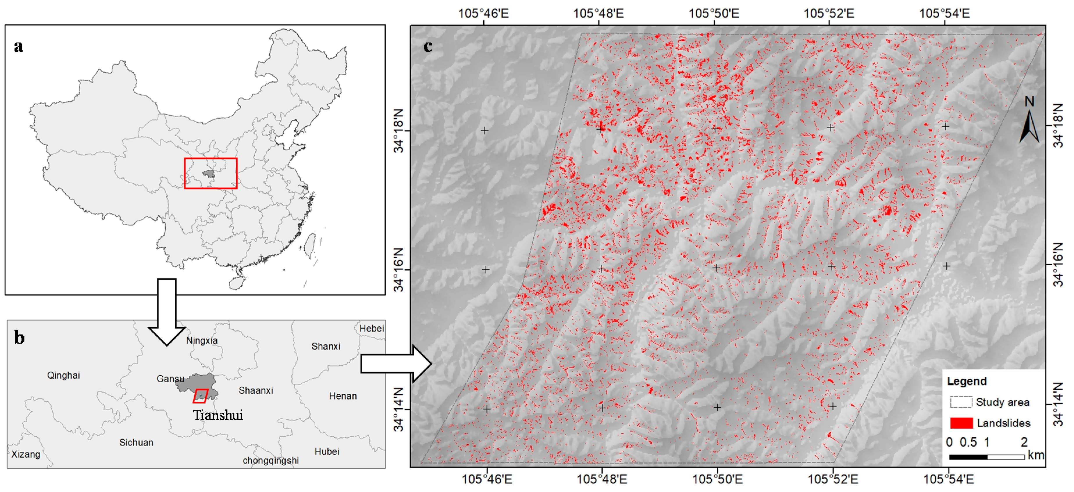
The study area is located in Tianshui city, Gansu Province, China (Figure 1), which lies the Loess Plateau. The total area of landslides is 6.34 km2. Mean annual precipitation is 512 mm in Tianshui. From July 20 to 22 in 2013, Tianshui experienced heavy rainfall reaching 241 mm in a period of 49 h [36], which is very rare in this semi-arid region. This heavy rainfall event in July 2013 triggered thousands of landslides over a large region.
3. Data and Method
3.1. Data Source
3.1.1. High Resolution Satellite Images
The GeoEye-1 image was acquired on 8 October 2013, two months after the July 2013 Tianshui rainfall-triggered landslide event. The panchromatic band has a nominal spatial resolution of 0.5 m. The multispectral bands are 1.65 m ground sampling distance with four bands in near-infrared (NIR), red, green, and blue bands. Covering an area of 128 km2, the GeoEye-1 image is in the WGS84 coordinate system, with a longitude of 105°44′48″–105°55′45″E and a latitude of 34°13′11″–34°19′20″N.
3.1.2. Landslide Inventory Maps
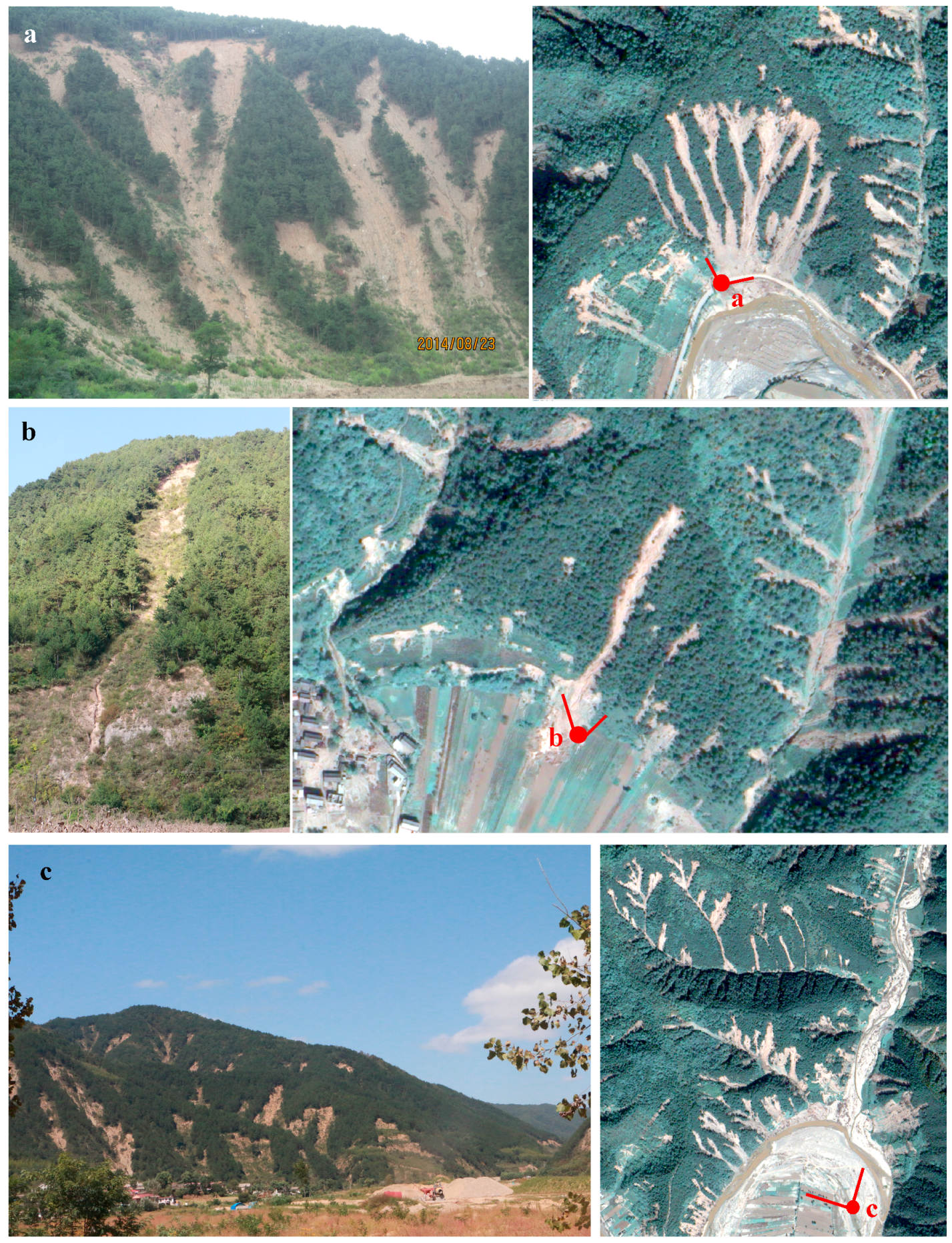
The inventory of the 2013 Tianshui rainfall-triggered landslides was manually produced from the GeoEye-1 image and validated by field reconnaissance. Up to 17,515 landslides triggered by the heavy rainfall were delineated as individual solid polygons in the study area (Figure 1). According to the classification scheme proposed by [37] and modified by [38], most landslides in this study area are shallow debris avalanches and debris flows (Figure 2). Debris avalanches are located on slopes and debris flows are located in valley bottoms, which were transformed from landslide debris on slopes. During our field reconnaissance, we found depth of most debris avalanches are ≈1 m. All types of landslides in this work are defined as landslides. Several field surveys were carried out after the event and landslide photos were taken in August 2014 or September 2018 (Figure 2) to validate interpretation.
3.1.3. Preparation of Training and Validation Datasets
The spatial resolution of GeoEye-1 used in this work is 0.5 m in panchromatic and 1.65 m in multi-spectral bands. Using the Gram-Schmidt Spectral Sharpening module in ENVI 4.8, we pansharpened the multispectral and panchromatic bands. The size of pansharpened image is 33,368 × 22,900 pixels with a 0.5 m ground sampling distance. In order to simplify the model and improve speed of model training, we converted the 16-bit original image into 8-bit and only used three spectral bands (near infrared, red, and green) to perform the analysis. The landslide inventory maps were converted to raster with the same resolution as the pansharpened image. The label for landslides was encoded as 1 and the non-landslide pixels encoded as 0.
Training of convolutional neural networks (CNN) requires many thousands annotated training samples. As the CNN model operates on square input patches, the satellite image and inventory map layer were divided to 1443 patches with size of 600 × 600 pixels. In total, 80% of these image patches (1154) were randomly selected as training data to train the model. The remaining 20% of image patches (289) were taken as the model validation area to evaluate the performance of the models.
3.2. Proposed Models
3.2.1. Baseline Model
The U-Net network is presented by semantic segmentation task for bio-medical image segmentation [34]. It is designed for a small training dataset with training strategy that relies on the strong use of data augmentation, in order to use the available annotated samples more efficiently. U-Net is a deep learning framework based on fully convolutional networks and comprises two parts: a contracting path (an encoder) to capture context via a compact feature map and an expanding path (a decoder) for precise localization. The U-Net combines low layer context information and high layer semantic information through skip connection to improve image segmentation accuracy. In this paper, we used U-Net as a baseline model to compare its performance with the ResU-Net.
3.2.2. Residual Learning Block
Generally, deeper layers in deep learning models could have better performances, but deeper layers can also lead to model degradation. To settle this problem, He et al. [27] presented a residual learning framework to ease the training of networks and solve training error with increasing depth of networks. The residual learning block is
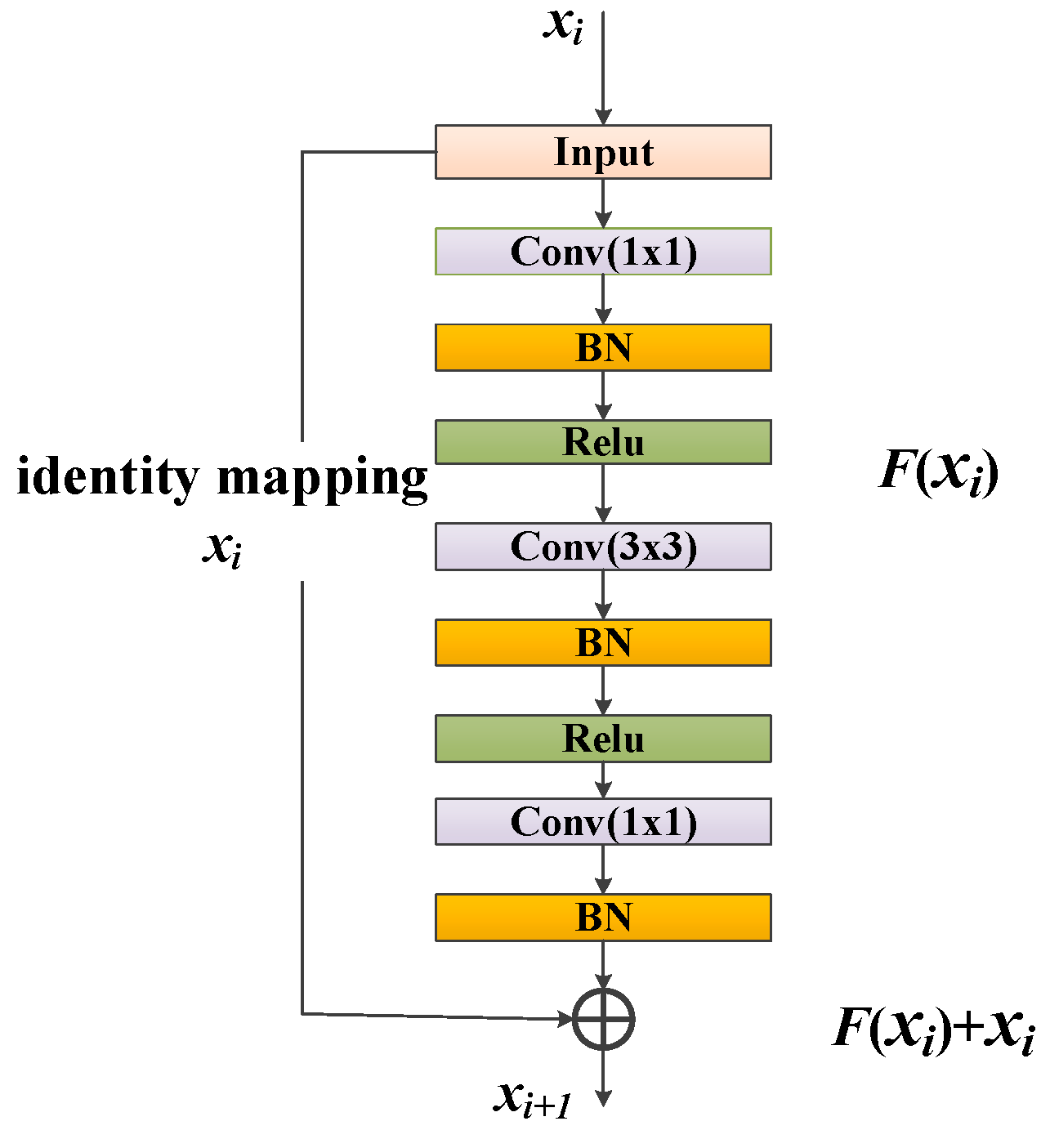
where xi and y are input and output vectors of the i-th residual block considered, and function F(x) represents the residual mapping to be learned. In this study, skip connection was implemented between the first convolutional layer and the third convolutional layer and performs identity mapping between input vectors and output vectors (Figure 3). Outputs of each residual block were added to the outputs of the stacked convolutional layers.
y = F(xi) + xi
In this work, a residual block includes three convolutional layers and three batch normalization (BN) layers [39]. The first and second convolutional layers are following a rectified linear unit (ReLU) activation layer after the BN layer as shown in Figure 3. The (i + 1)-th residual learning block considers the i-th input residual vectors to optimize training progress [27].
3.2.3. Proposed ResU-Net
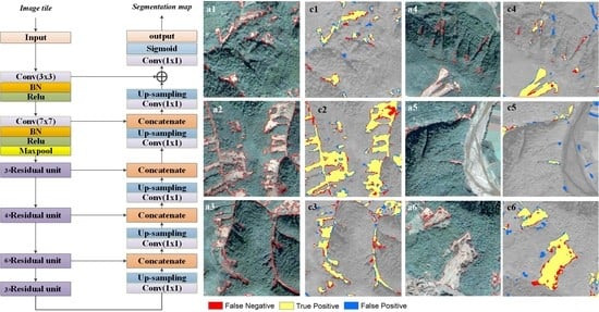
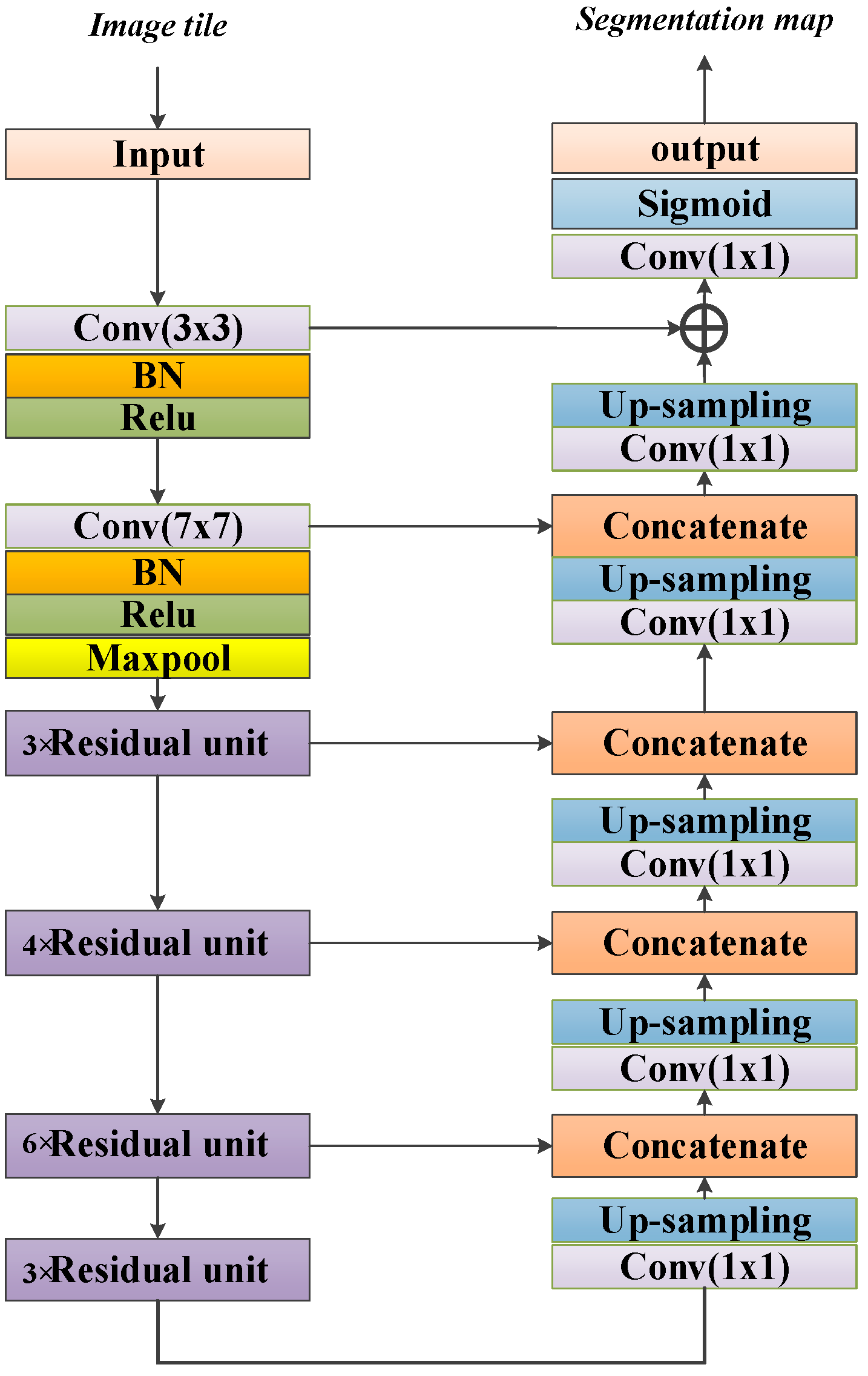
In order to solve training degradation problem with increasing depth of network layers, we adopted residual learning block to replace every convolutional layer of the encoding path of U-Net baseline model. The network architecture of the ResU-Net is illustrated in Figure 4 and Table 1, which consists of an encoding path (left side) and a decoding path (right side).
The encoding path comprises an input unit, a head unit, and a residual unit. The head unit includes two convolutional layers, followed by a BN layer and a ReLU. The first residual unit (Residual unit_1 in Table 1) includes three residual blocks stacked with nine convolutional layers. The second residual unit (Residual unit_2 in Table 1) consists of four residual blocks stacked with 12 convolutional layers. The third residual unit (Residual unit_3 in Table 1) includes six residual blocks stacked with 18 convolutional layers. The fourth residual unit (Residual unit_4 in Table 1) includes three residual blocks stacked with nine convolutional layers. Default parameters in the structures of the residual units were used in this work [27]. Down-sampling of feature map was performed by conv12, conv24, and conv42 with a stride of 2, while doubling the number of feature channels.
The decoding path contains repeated applications of four concatenate blocks, one addition block, and an output unit. Each concatenate block consists of one 1 × 1 convolution and an up-sampling of the feature map that halves the number of feature channels. We built a concatenation between output feature maps after each concatenate block and output feature maps from the corresponding residual unit of encoding path. At the final layer of the decoding path, a 1 × 1 convolution filter and a Sigmoid activation layer were used to map segmentation results for a binary classification. The copy and crop were implemented between output feature of every residual block and convolutional layer of decoding path. The copy and cropping are necessary for multi-scale feature fusion. As shown in Table 1, the ResU-Net has 56 convolutional layers.
3.3. Implementation of Training
The ResU-Net model and U-Net were implemented using the PyTorch framework. All the codes used in this research are available as supplementary material on GitHub: https://github.com/WenwenQi/Deep-Residual-U-Net-for-extracting-landslides. Additionally, all models were optimized by the Mini-batch Stochastic Gradient Descent algorithm [40]. The performance of the deep learning algorithms heavily relies on training dataset, layer depth, input window sizes, and training strategies [29]. We set the initial learning rate as 0.001, which was then decayed by a rate of 0.1 for every 20 epochs. The total epochs were 200. We trained the ResU-Net model and U-Net model with a mini-batch size of 5 on a NVIDIA™ GeForce GTX 1080 Ti GPU (12GB memory). Momentum was high (0.9) and weight decay was 5 × 10⁻⁵. There were 1148 fixed-size training image tiles (600 × 600 pixels) available for training. In this work, data augmentation was used during training, for example, flipping image horizontally, vertically, and horizontally and vertically, in order to increase training data volume and avoid the over-fitting problem.
In this work, we used the Binary Cross Entropy loss function (BCELoss), which can be described as:
where N is the batch size, ln is loss of each sample of the mini-batch, and wn is a manual rescaling weight given to the loss of each batch element in the training. By default, the losses (l(x, y)) were averaged over each loss element in the batch, which was used for measuring the error of a reconstruction in an auto-encoder.
l(x, y) = L = {l1, … lN}T,
ln = −wn [yn · log xn + (1 − yn) · log (1 − xn)],
We used the Kaiming Uniform initialization method [41] to initialize weights of the model, which takes Rectified Linear Unit and Parametric Rectified Linear Unit (ReLU/PReLU) into account. This method is a robust initialization tool allowing for extremely deep models to converge.
By using the models, a series of landslide probability maps were produced based on the validating area. All output probability maps were tiles with size of 600 × 600 pixels. We added geo-transformation and projection information for every image tile of probability map and mosaic all image tiles using GDAL/OGR library.
3.4. Evaluation
Evaluation was carried out in the validating part of the study area using manually interpreted landslides. To evaluate the performance of the proposed ResU-Net, we calculated recall, precision, and F1. Recall is the fraction of the total reference landslides that are actually detected. Precision is the fraction of the total detected landslides that are really landslides. Recall and Precision are evenly weighted used F-measure (F1). The F1 score was used as a standard criterion to evaluate model performance by combining the precision and recall. The F1 score is simply a way to combine the precision and recall. The F1 score can be calculated by using harmonic mean of the precision and recall. It ranges from 0 to 1. The higher the F1, the better the predictions.
where TP is true positive, which is correctly identified landslides; FN is false negative, which is true landslides but is omitted by the method; and FP is false positive, which is not landslides but is mistakenly detected as landslides by the method.
Recall = TP/(TP + FN),
Precision = TP/(TP + FP),
F1 = (2 · R · P)/(R + P), (R: Recall, P: Precision),
4. Results
In Table 2, we can see that the proposed ResU-Net have the best results in terms of precision, recall, and F1. Precision in the ResU-Net improved slightly (0.03) compared to the U-Net model. Recall in the ResU-Net improved the most than the U-Net model (0.13 higher than U-Net). F1 in the ResU-Net is 0.09 higher than the U-Net. With the same hardware, it took ≈29 and ≈72 h to train the U-Net and the ResU-Net models, respectively. After training, both models need similar testing time (2–3 s) for each image tile (600 × 600 pixels).
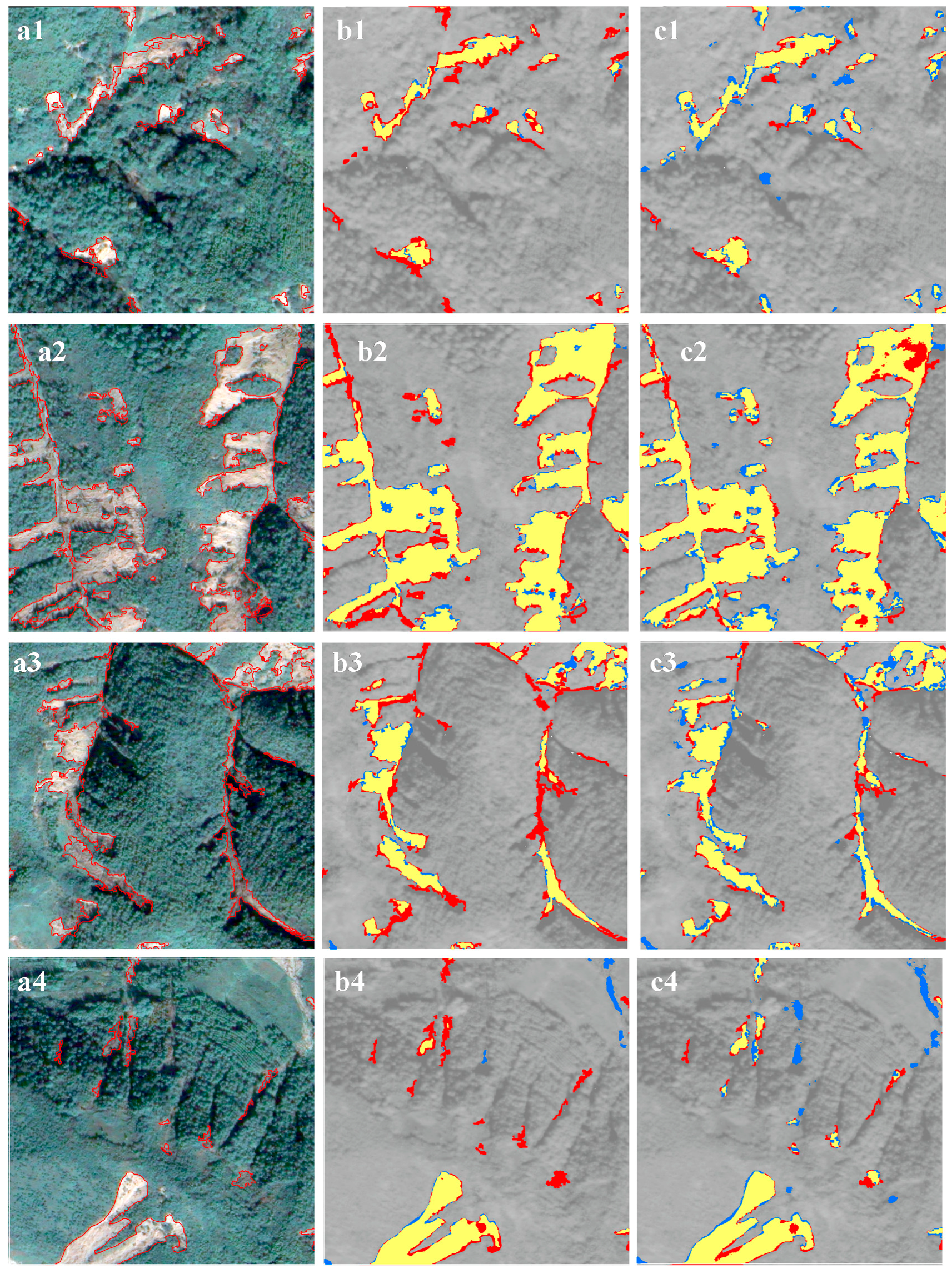
We further showed mapping results of the two models (the U-Net and the ResU-Net) in the validation area (Figure 5). The yellow, red, and blue polygons are corrected landslides, omission, and commission errors, respectively.
Although all methods can correctly detect most landslides (yellow polygons in Figure 5), they have difficulty in detecting small size landslides (Figure 5b1–b6 and Figure 5c1–c6). The ResU-Net model is better than the U-Net model for extraction of small and slender landslide polygons (Figure 5b2,b3 and Figure 5c2,c3).
Compared to the ResU-Net, the U-Net has difficulty in delineating landslide boundaries and has more omission errors (red polygons in Figure 5b1–b6). As follows in Figure 5b6, the U-Net model has more omission errors around boundaries of the large size landslides.
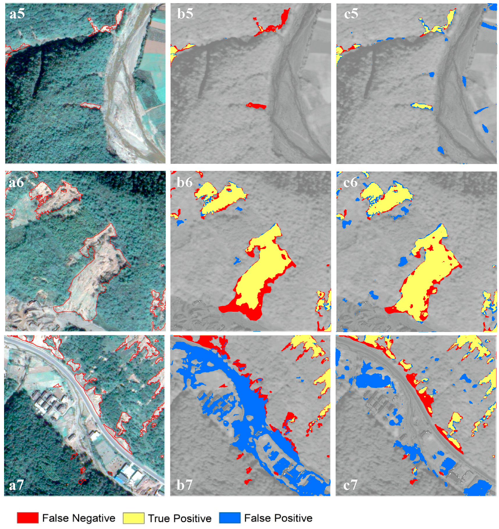
As the GeoEye-1 image we used has very high spatial resolution (0.5 m), landslides are spectrally heterogeneous ground features. Floodplains in this image look very similar with landslides and pose a challenge in identifying landslides. The U-Net model has more omission errors on floodplains (Figure 5b5). The problem with very high spatial resolution images like this is that the same ground features could have different spectral values, whereas different ground features are spectrally similar. A few omission errors and more commission errors occur for the ResU-Net along the floodplains (Figure 5c5). In Figure 5b7,c7, we can see that both models have difficulties in identifying landslides from roads and buildings. However, more false positives and false negatives occur under the U-Net model than the proposed ResU-Net.
5. Discussion
5.1. Model Comparisons
In this model, we proposed a ResU-Net by integrating the U-Net [34] and the residual learning algorithms [27]. To identify landslides, feature selection (such as NDVI, textural information) is a crucial step in traditional machine learning models [10,13]. Selecting the most efficient features as input for machine learning models heavily relies on expert experiences. Deep learning models were developed on the basis of large datasets and high computing power. When we train deep learning models, model inputs are image patches. These image patches are spectral features of three bands (near infrared, red, and green) and semantic features can be automatically generated and used in identifying landslides. Converting low-level (spectral) features to high-level (semantic) features is a major advantage of deep learning models over traditional machine learning models.
Although deep learning methods have the advantage of automatic semantic feature extraction, they could face the problem of training degradation with limited annotated training samples. Most existing methods to identify landslides use many environmental factors and a few convolutional layers (four- or seven-layer depth) to avoid model degradation [28,29,30]. By adopting the residual learning to every convolutional layer of the encoding path in the model, the proposed ResU-Net model can avoid model degradation to reach higher accuracy than the U-Net (F1 improved by 0.09). By integrating the residual learning units, the ResU-Net could have up to 56 convolutional layers without training degradation. In addition, the ResU-Net applied a shortcut connection strategy to pass some high-resolution low-level features to the final classification module, which could use image information more efficiently. Compared with the U-Net model, the proposed ResU-Net performs better in delineating landslide boundaries (Figure 5).
Output of these models (the ResU-Net and the U-Net) are landslide probability maps. Higher values in these probability maps indicate more confidence in predicting landslides. To get the final predicted binary landslide map, we have to use a threshold to transfer the landslide probability map. Pixels with model output values larger than the defined threshold will be assigned as landslide pixels, otherwise are non-landslide pixels. In general, lower thresholds may successfully detect more true landslides, but we risk assigning false pixels as landslides (more commission errors). This will lead to lower precision and F1, but higher recall. In contrast, higher thresholds will result in less predicted landslide pixels (omission errors), leading to lower recall, F1, and higher precision. As determining the threshold is not the scope of this work, we used thresholds with balanced precision, recall, and F1 scores for all models.
5.2. Limitations of the Model
Landslides are earth surface processes of various spatial scales ranging from a few square meters to many thousands of square meters. Both deep learning models did not consider landslide scale differences, and they have poor performances in detecting small landslides. During semantic feature extractions at the convolution and pooling procedures, small landslides of a few image pixels in deep learning models could become blurred. Building image pyramids and introducing pyramid pooling algorithms are two possible ways to solve this problem [29,31].
High accuracy of extracting landslides in this region may be partially because the proposed algorithm was applied on a rural area. Models can easily discriminate landslides from dense vegetation, but there are bare lands in our study area, which are spectrally similar to landslides. It is also possible that by adding a high spatial resolution DEM, the model could easily discriminate landslides from flat floodplains [42]. However, the optical image in this work has a spatial resolution of 0.5 m and a DEM with such high spatial resolution is very difficult to acquire. Acquiring very high spatial resolution DEM may also be a problem in other parts of mountain regions. Therefore, extracting landslides from bare spectral information is a worthwhile effort.
Landslide extraction using deep learning models requires large amounts of label data and raw images. To perform the ResU-Net and U-Net, we divided the entire study area into 1443 image patches with size of 600 × 600 pixels. We then selected 80% of the study area, i.e., 1154 image patches, to train both models. In total, the amount of training data is very large, 1154 × 600 × 600 × 4 pixel values (three optical bands and a layer with landslide labels). As the GeoEye-1 data is 16-bit floating data, there are at > 1.6 billion floating values to be used as training data. We trained this amount of training data with a server (Ubuntu 16.04 and Intel® Xeon® CPU E5-2620) and accelerated by the NVIDIA™ GeForce GTX 1080 Ti GPU (12GB memory). These requirements for label data and hardware may limit its use to some extent. Besides, there are some omission and commission errors in our results (Figure 5), which indicate that other information other than spectral information (such as DEM) should be used to further improve model performances.
5.3. Potential Applications
With more high spatial resolution images available in the future, large volumes of very high-resolution images will be available for regional landslide mapping. During post-disaster assessment, fast mapping of landslides could be urgently needed. This method can provide a possible solution in fast landslide mapping triggered by major earthquakes or extreme rainfalls. By using NVIDIA™ GPU, an image tile with size of 600 × 600 pixels can be automatically mapped landslides per 3 s. This fast mapping method may play an important role in landslide inventory mapping in the future.
The proposed method for identifying landslides could also be used in other types of landslide mapping. Take the landslide susceptibility mapping as an example, which is similar with landslide detection of this work. Both of them use landslides as model dependent. The differences are instead of using spectral bands from remote sensing images, landslide susceptibility mapping uses environmental layers such as lithology, slope, and land use cover type [43]. In the future, if these environmental factors are considered, the model proposed in this paper could be readily applied to landslide susceptibility and hazard mapping.
6. Conclusions
Automatic mapping of landslides from optical images could greatly benefit generation of regional landslide inventories. Although existing deep learning methods can extract features efficiently in landslide identifications, they may face training degradation with limited annotated samples. To solve this problem, we proposed the ResU-Net for automatic landslide mapping, which is built based on the architecture of U-Net by integrating residual learning algorithms. By hybriding both algorithms, this proposed method achieves higher accuracy in a spatially heterogeneous mountain region than the baseline U-Net model by using 3-band optical images. The higher accuracy in the ResU-Net indicates that this model performs better in avoiding model degradation with limited annotated training landslide samples. The ResU-Net also has promising potential in other types of regional landslide studies, such as landslide susceptibility and hazard mapping by integrating environmental information.
Supplementary Materials
Python code, input image data, and manually interpreted landslides can be accessed at: https://github.com/WenwenQi/Deep-Residual-U-Net-for-extracting-landslides.
Author Contributions
W.Q. designed the framework of this work and wrote the manuscript. W.Q. and M.W. conducted numerical analyses. W.Y. and C.M. provided all remote sensing images, landslide inventory, and field photos. C.X. discussed the paper and made contributions to manuscript modifications. All authors have read and agreed to the published version of the manuscript.
Funding
This research was jointly funded by the National Institute of Natural Hazards, Ministry of Emergency Management of China (former Institute of Crustal Dynamics, China Earthquake Administration) Research Fund (ZDJ2020-01) and the National Key Research and Development Project of China (2016YFC0501604-05, 2018YFB0505501).
Acknowledgments
The landslide inventory is produced by a joint effort between Wentao Yang, Chao Ma, Muyang Li, and Zhisheng Dai from Beijing Forestry University. The authors would like to thank this team for offering landslide inventory data. We also express our gratitude to the anonymous reviewers for their comments and suggestions that improved the quality of our paper.
Conflicts of Interest
The authors declare no conflict of interest.
References
- Cui, P.; Chen, X.; Zhu, Y.; Su, F.; Wei, F.; Han, Y.; Liu, H.; Zhuang, J. The Wenchuan Earthquake (May 12, 2008), Sichuan Province, China, and resulting geohazards. Nat. Hazards 2011, 56, 19–36. [Google Scholar] [CrossRef]
- Huang, R.; Li, W. Analysis of the geo-hazards triggered by the 12 May 2008 Wenchuan Earthquake, China. Bull. Eng. Geol. Environ. 2009, 68, 363–371. [Google Scholar] [CrossRef]
- Qi, S.; Xu, Q.; Lan, H.; Zhang, B.; Liu, J. Spatial distribution analysis of landslides triggered by 2008.5.12 Wenchuan Earthquake, China. Eng. Geol. 2010, 116, 95–108. [Google Scholar] [CrossRef]
- Xu, C.; Xu, X.; Yao, X.; Dai, F. Three (nearly) complete inventories of landslides triggered by the May 12, 2008 Wenchuan Mw 7.9 earthquake of China and their spatial distribution statistical analysis. Landslides 2014, 11, 441–461. [Google Scholar] [CrossRef] [Green Version]
- Chen, Y.; Chang, K.; Wang, S.; Huang, J.; Yu, C.; Tu, J.; Chu, H.; Liu, C. Controls of preferential orientation of earthquake- and rainfall-triggered landslides in Taiwan’s orogenic mountain belt. Earth Surf. Process. Landf. 2019, 44, 1661–1674. [Google Scholar] [CrossRef]
- Keefer, D. Investigating landslides caused by earthquakes–a historical review. Surv. Geophys. 2002, 23, 473–510. [Google Scholar] [CrossRef]
- Harp, E.; Keefer, D.; Sato, H.; Yagi, H. Landslide inventories: the essential part of seismic landslide hazard analyses. Eng. Geol. 2011, 122, 9–21. [Google Scholar] [CrossRef]
- Mondini, A.; MarChesini, I.; Rossi, M.; Chang, K.; Pasquariello, G.; Guzzetti, F. Bayesian framework for mapping and classifying shallow landslides exploiting remote sensing and topographic data. Geomorphology 2013, 201, 135–147. [Google Scholar] [CrossRef]
- Keyport, R.; Oommen, T.; Martha, T.; Sajinkumar, K.; Gierke, J. A comparative analysis of pixel- and object-based detection of landslides from very high-resolution images. Int. J. Appl. Earth Obs. Geoinf. 2018, 64, 1–11. [Google Scholar] [CrossRef]
- Mondini, A.; Guzzetti, F.; Reichenbach, P.; Rossi, M.; Cardinali, M.; Ardizzone, F. Semi-automatic recognition and mapping of rainfall induced shallow landslides using optical satellite images. Remote Sens. Environ. 2011, 115, 1743–1757. [Google Scholar] [CrossRef]
- Yang, W.; Shi, P.; Liu, L. Dentifying landslides using binary logistic regression and landslide detection index, in Proceedings Earthquake-Induced Landslides, Kiryu, Japan. Springer Berl. Heidelb. 2012, 781–789. [Google Scholar] [CrossRef]
- Yang, W.; Wang, M.; Shi, P. Using MODIS NDVI time series to identify geographic patterns of landslides in vegetated regions. IEEE Geosci. Remote Sens. Lett. 2013, 10, 707–710. [Google Scholar] [CrossRef]
- Lu, P.; Qin, Y.; Li, Z.; Mondini, A.; Casagli, N. Landslide mapping from multi-sensor data through improved change detection-based Markov random field. Remote Sens. Environ. 2019, 231, 111235. [Google Scholar] [CrossRef]
- Stumpf, A.; Kerle, N. Object-oriented mapping of landslides using Random Forests. Remote Sens. Environ. 2011, 115, 2564–2577. [Google Scholar] [CrossRef]
- GSP, 216. Learning Module 6.1: Object Based Classification. Geospatial Science at Humboldt State University. Available online: http://gsp.humboldt.edu/OLM/Courses/GSP_216_Online/lesson6-1/object.html (accessed on 20 December 2019).
- Zhu, X.; Tuia, D.; Mou, L.; Xia, G.; Zhang, L.; Xu, F.; Fraundorfer, F. Deep Learning in Remote Sensing: A Comprehensive Review and List of Resources. IEEE Geosci. Remote Sens. Mag. 2017, 5, 8–36. [Google Scholar] [CrossRef] [Green Version]
- Duric, U.; Marjanovic, M.; Radic, Z.; Abolmasov, B. Machine learning based landslide assessment of the Belgrade metropolitan area: Pixel resolution effects and a cross-scaling concept. Eng. Geol. 2019, 256, 23–38. [Google Scholar] [CrossRef]
- Jean, N.; Burke, N.; Xie, M.; Davis, W.; Lobell, D.; Ermon, S. Combining satellite imagery and machine learning to predict poverty. Science 2016, 353, 790–794. [Google Scholar] [CrossRef] [Green Version]
- DeVries, P.; Viegas, F.; Wattenberg, M.; Meade, B. Deep learning of aftershock patterns following large earthquakes. Nature 2018, 560, 632–634. [Google Scholar] [CrossRef]
- Ham, Y.; Kim, J.; Luo, J. Deep learning for multi-year ENSO forecasts. Nature 2019, 573, 568–572. [Google Scholar] [CrossRef]
- Hu, Q.; Zhou, Y.; Wang, S.; Wang, F.; Wang, H. Improving the accuracy of landslide detection in“off-site” area by machine learning model portability comparison: a case study of Jiuzhaigou Earthquake, China. Remote Sens. 2019, 11, 2530. [Google Scholar] [CrossRef] [Green Version]
- Piralilou, S.; Shahabi, H.; Jarihani, B.; Ghorbanzadeh, O.; Blaschke, T.; Gholamnia, K.; Raj Meena, S.; Aryal, J. Landslide detection using multi-scale image segmentation and different machine learning models in the Higher Himalayas. Remote Sens. 2019, 11, 2575. [Google Scholar] [CrossRef] [Green Version]
- Ye, C.; Li, Y.; Cui, P.; Liang, L.; Pirasteh, S.; Marcato, J.; Gonçalves, W.; Li, J. Landslide detection of hyperspectral remote sensing data based on deep learning with constrains. IEEE J. Sel. Top. Appl. Earth Obs. Remote Sens. 2019, 12, 5047–5060. [Google Scholar] [CrossRef]
- Prakash, N.; Manconi, A.; Loew, S. Mapping landslides on EO data: performance of deep learning models vs. traditional machine learning models. Remote Sens. 2020, 12, 346. [Google Scholar] [CrossRef] [Green Version]
- Yu, B.; Chen, F.; Xu, C. Landslide detection based on contour-based deep learning framework in case of national scale of Nepal in 2015. Comput. Geosci. 2020, 135, 104388. [Google Scholar] [CrossRef]
- Zhu, L.; Huang, L.; Fan, L.; Huang, J.; Huang, F.; Chen, J.; Zhang, Z.; Wang, Y. Landslide susceptibility prediction modeling based on remote sensing and a novel deep learning algorithm of a cascade-parallel recurrent neural network. Sensors 2020, 20, 1576. [Google Scholar] [CrossRef] [Green Version]
- He, K.; Zhang, X.; Ren, S.; Sun, J. Deep residual learning for image recognition. In Proceedings of the 2016 IEEE Conference on Computer Vision and Pattern Recognition (CVPR), Las Vegas, NV, USA, 27–30 June 2016; pp. 770–778. [Google Scholar] [CrossRef] [Green Version]
- Chen, Z.; Zhang, Y.; Ouyang, C.; Zhang, F.; Ma, J. Automated Landslides Detection for Mountain Cities Using Multi-Temporal Remote Sensing Imagery. Sensors 2018, 18, 821. [Google Scholar] [CrossRef] [Green Version]
- Ghorbanzadeh, O.; Blaschke, T.; Gholamnia, K.; Meena, S.; Tiede, D.; Aryal, J. Evaluation of Different Machine Learning Methods and Deep-Learning Convolutional Neural Networks for Landslide Detection. Remote Sens. 2019, 11, 196. [Google Scholar] [CrossRef] [Green Version]
- Sameen, M. and Pradhan, B. Landslide Detection Using Residual Networks and the Fusion of Spectral and Topographic Information. IEEE Access 2019, 7, 114363–114373. [Google Scholar] [CrossRef]
- Lei, T.; Zhang, Y.; Lv, Z.; Li, S.; Liu, S.; Nandi, A. Landslide inventory mapping from bitemporal images using deep convolutional neural networks. IEEE Geosci. Remote Sens. Lett. 2019, 16, 982–986. [Google Scholar] [CrossRef]
- Wang, Y.; Fang, Z.; Hong, H. Comparison of convolutional neural networks for landslide susceptibility mapping in Yanshan County, China. Sci. Total Environ. 2019, 666, 975–993. [Google Scholar] [CrossRef] [PubMed]
- Huang, F.; Zhang, J.; Zhou, C.; Wang, Y.; Huang, J.; Zhu, L. A deep learning algorithm using a fully connected sparse autoencoder neural network for landslide susceptibility prediction. Landslides 2019, 17, 217–229. [Google Scholar] [CrossRef]
- Ronneberger, O.; Fischer, P.; Brox, T. U-Net: Convolutional Networks for Biomedical Image Segmentation. In Medical Image Computing and Computer-Assisted Intervention—MICCAI 2015; Navab, N., Hornegger, J., Wells, W.M., Frangi, A.F., Eds.; Springer International Publishing: Berlin/Heidelberg, Germany, 2015; pp. 234–241. [Google Scholar]
- Liu, P.; Wei, Y.; Wang, Q.; Chen, Y.; Xie, J. Research on Post-Earthquake Landslide Extraction Algorithm Based on Improved U-Net Model. Remote Sens. 2020, 12, 894. [Google Scholar] [CrossRef] [Green Version]
- Peng, J.; Fan, Z.; Wu, D.; Zhuang, J.; Dai, F.; Chen, W.; Zhao, C. Heavy rainfall triggered loess–mudstone landslide and subsequent debris flow in Tianshui, China. Eng. Geol. 2015, 186, 79–90. [Google Scholar] [CrossRef]
- Cruden, D.M.; Varnes, D.J. Landslide Types and Processes, Special Report, Transportation Research Board. Proc. Natl. Acad. Sci. USA 1996, 247, 36–75. [Google Scholar]
- Highland, L.M.; Bobrowsky, P. The Landslide Handbook—A Guide to Understanding Landslides; United States Geological Survey: Reston, VA, USA, 2008; Volume 1325, p. 129.
- Ioffe, S.; Szegedy, C. Batch normalization: Accelerating deep network training by reducing internal covariate shift. arXiv 2015, arXiv:1502.03167. [Google Scholar]
- Hinton, G.; Srivastava, N.; Swersky, K. Neural Networks for Machine Learning Lecture 6a Overview of Mini-Batch Gradient Descent. 2012. Available online: http://59.80.44.49/www.cs.toronto.edu/~hinton/coursera/lecture6/lec6.pdf (accessed on 10 August 2019).
- He, K.; Zhang, X.; Ren, S.; Sun, J. Delving Deep into Rectifiers: Surpassing Human-Level Performance on ImageNet Classification. In Proceedings of the 2015 IEEE International Conference on Computer Vision (ICCV), Santiago, Chile, 7–13 December 2015; pp. 1026–1034. [Google Scholar] [CrossRef] [Green Version]
- Tang, C.; Tanyas, H.; van Westen, C.; Tang, C.; Fan, X.; Jetten, V.G. Analysing post-earthquake mass movement volume dynamics with multi-source DEMs. Eng. Geol. 2019, 248, 89–101. [Google Scholar] [CrossRef]
- Reichenbach, P.; Rossi, M.; Malamud, B.; Mihir, M.; Guzzetti, F. A review of statistically-based landslide susceptibility models. Earth Sci. Rev. 2018, 180, 60–91. [Google Scholar] [CrossRef]
Figure 1.
Maps of the study area. (a,b) Location of the study area and (c) the landslide inventory map and boundary of study area.
Figure 1.
Maps of the study area. (a,b) Location of the study area and (c) the landslide inventory map and boundary of study area.

Figure 2.
Landslide photos (a–c) taken during field reconnaissance. Locations and directions to take these photos are shown on GeoEye-1 RGB (Red-Green-Blue) composite images on the right column.
Figure 2.
Landslide photos (a–c) taken during field reconnaissance. Locations and directions to take these photos are shown on GeoEye-1 RGB (Red-Green-Blue) composite images on the right column.

Figure 3.
Residual learning block.

Figure 4.
Architecture of ResU-Net.

Figure 5.
Comparison of results in validation area using different models. (a1–a7) GeoEye-1 images with ground truth of landslides (red boundary polygons), extracted landslides by the UNet (b1–b7) and the ResU-Net (c1–c7). The yellow, red, and blue polygons are corrected landslides, omission, and commission errors, respectively.


Table 1.
Network architecture of ResU-Net.
| Unit | Convolutional Layer | Filter Size, Channels | Output Size (Width × Height × Channels) | |
|---|---|---|---|---|
| Input | 600 × 600 × 3 | |||
| Encoding path | Head | conv 1 | 3 × 3, 64 | 600 × 600 × 64 |
| conv 2 | 7 × 7, 64 | 300 × 300 × 64 | ||
| max pool | 3 × 3, 64 | 150 × 150 × 64 | ||
| Residual unit_1 | conv 3-11 | 150 × 150 × 256 | ||
| Residual unit_2 | conv 12-23 | 75 × 75 × 512 | ||
| Residual unit_3 | conv 24-41 | 38 × 38 × 1024 | ||
| Residual unit_4 | conv 42-50 | 19 × 19 × 2048 | ||
| Decoding path | Concatenate_1 | conv 51 | 1 × 1, 1024 | 38 × 38 × 1024 |
| Concatenate_2 | conv 52 | 1 × 1, 512 | 75 × 75 × 512 | |
| Concatenate_3 | conv 53 | 1 × 1, 256 | 150 × 150 × 256 | |
| Concatenate_4 | conv 54 | 1 × 1, 64 | 300 × 300 × 64 | |
| Addition | conv 55 | 1 × 1, 64 | 600 × 600 × 64 | |
| Output | conv 56 | 1 × 1, 3 | 600 × 600 × 3 | |
Table 2.
Assessment of identified landslides.
| Model | Precision (%) | Recall (%) | F1 (%) |
|---|---|---|---|
| U-Net | 0.93 | 0.70 | 0.80 |
| ResU-Net | 0.96 | 0.83 | 0.89 |
© 2020 by the authors. Licensee MDPI, Basel, Switzerland. This article is an open access article distributed under the terms and conditions of the Creative Commons Attribution (CC BY) license (http://creativecommons.org/licenses/by/4.0/).
Share and Cite
MDPI and ACS Style
Qi, W.; Wei, M.; Yang, W.; Xu, C.; Ma, C. Automatic Mapping of Landslides by the ResU-Net. Remote Sens. 2020, 12, 2487. https://0-doi-org.brum.beds.ac.uk/10.3390/rs12152487
AMA Style
Qi W, Wei M, Yang W, Xu C, Ma C. Automatic Mapping of Landslides by the ResU-Net. Remote Sensing. 2020; 12(15):2487. https://0-doi-org.brum.beds.ac.uk/10.3390/rs12152487
Chicago/Turabian StyleQi, Wenwen, Mengfei Wei, Wentao Yang, Chong Xu, and Chao Ma. 2020. "Automatic Mapping of Landslides by the ResU-Net" Remote Sensing 12, no. 15: 2487. https://0-doi-org.brum.beds.ac.uk/10.3390/rs12152487
Note that from the first issue of 2016, this journal uses article numbers instead of page numbers. See further details here.