Article

Estimating Structure and Biomass of a Secondary Atlantic Forest in Brazil Using Fourier Transforms of Vertical Profiles Derived from UAV Photogrammetry Point Clouds

1
Department of Agricultural Engineering, Federal University of Sergipe, São Cristóvão SE 49100-000, Brazil
2
Canopy Remote Sensing Solutions, Florianópolis SC 88032, Brazil
3
Department of Forest Science, Federal University of Espírito Santo, Jerônimo Monteiro ES 29550, Brazil
4
Department of Biological and Agricultural Engineering, Texas A&M University, College Station, TX 77840, USA
5
Jet Propulsion Laboratory, California Institute of Technology, Pasadena, CA 91109, USA
6
Water Resources Program, Federal University of Sergipe, São Cristóvão SE 49100-000, Brazil
7
State Secretariat for Urban Development and Sustainability, Aracaju SE 49030, Brazil
*
Author to whom correspondence should be addressed.
Remote Sens. 2020, 12(21), 3560; https://0-doi-org.brum.beds.ac.uk/10.3390/rs12213560
Submission received: 25 September 2020 / Revised: 17 October 2020 / Accepted: 27 October 2020 / Published: 30 October 2020
(This article belongs to the Special Issue 3D Point Clouds in Forest Remote Sensing)

Abstract

:
Knowing the aboveground biomass (AGB) stock of tropical forests is one of the main requirements to guide programs for reducing emissions from deforestation and forest degradation (REDD+). Traditional 3D products generated with digital aerial photogrammetry (DAP) have shown great potential in estimating AGB, tree density, diameter at breast height, height, and basal area in forest ecosystems. However, these traditional products explore only a small part of the structural information contained in the 3D data, thus not leveraging the full potential of the data for inventory purposes. In this study, we tested the performance of 3D products derived from DAP and a technique based on Fourier transforms of vertical profiles of vegetation to estimate AGB, tree density, diameter at breast height, height, and basal area in a secondary fragment of Atlantic Forest located in northeast Brazil. Field measurements were taken in 30 permanent plots (0.25 ha each) to estimate AGB. At the time of the inventory, we also performed a digital aerial mapping of the entire forest fragment with an unmanned aerial vehicle (UAV). Based on the 3D point clouds and the digital terrain model (DTM) obtained by DAP, vertical vegetation profiles were produced for each plot. Using traditional structure metrics and metrics derived from Fourier transforms of profiles, regression models were fit to estimate AGB, tree density, diameter at breast height, height, and basal area. The 3D DAP point clouds represented the forest canopy with a high level of detail, regardless of the vegetation density. The metrics based on the Fourier transform of profiles were selected as predictors in all models produced. The best model for AGB explained 93% (R 2 = 0.93) of the biomass variation at the plot level, with an RMS error of 9.3 Mg ha 1 (22.5%). Similar results were obtained in the models fit for the tree density, diameter at breast height, height, and basal area, with R 2 values above 0.90 and RMS errors of less than 18%. The use of Fourier transforms of profiles with 3D products obtained by DAP demonstrated a high potential for estimating AGB and other forest variables of interest in secondary tropical forests, highlighting the value of UAV as a low-cost tool to assist the implementation of REDD+ projects in developing countries like Brazil.

Graphical Abstract

1. Introduction

Typically, aboveground biomass (AGB) estimates are made based on field campaigns that employ traditional forest inventory techniques. However, these campaigns have high operational and logistical costs, and demand a significant length of time for the work involved [1]. The rapid effects of climate change associated with the long length of time needed for data collection in the field can compromise the achievement of reducing emissions from deforestation and forest degradation (REDD+) programs [2,3,4]. REDD+ is a mechanism that has been proposed to provide financial incentives to developing countries to reduce emissions associated with forest loss and promote conservation, sustainable management, and increased forest carbon stocks [5]. The use of remote sensing data in the construction of models that facilitate estimating AGB in forests was one of the main guidelines indicated by the Intergovernmental Panel on Climate Change [6], with REDD+ mechanisms in developing countries such as Brazil [7]. With the use of remote sensing data, it is possible to model, map, and thus estimate carbon dynamics and other forest variables of interest with greater temporal efficiency and flexibility [8,9].
Remote sensing data associated with field inventory campaigns and modeling techniques have enabled increasingly reliable estimates of AGB [10,11,12]. Even where repeated inventory data are available, they have limited spatial coverage, which is insufficient for continuous spatial predictions of forest biomass [13]. This problem can be solved by associating the forest inventory with remote sensing data [14]. Three-dimensional products derived from light detection and ranging (LiDAR) have been used successfully in AGB estimation models in different types and forest formations [15,16,17,18]. However, despite the excellent accuracy of these models, the cost of this technique is still considered high, especially when the survey is carried out in large areas or when there is a need for different mappings in a short period of time, making it difficult or even impossible to use a LiDAR database. With the accelerated technological advancement of unmanned aerial vehicle (UAV) and image processing techniques, 3D products derived from digital aerial photogrammetry (DAP) have been showing satisfactory results in estimating AGB and other forest variables [19,20,21,22,23,24,25,26,27,28]. Several studies show that errors in forest attribute estimates with 3D products generated by DAP are comparable to those found using LiDAR data [29,30,31,32,33,34,35].
DAP is generated by overlapping image-matching algorithms, with their position and orientation parameters collected during the aircraft’s flight [21,22,24,26,27]. In addition to the lower cost and high spatial resolution (<1 m), the products generated by DAP in areas with open and fragmented vegetation are similar to LiDAR products [33]. On the other hand, in large areas of dense forests, the 3D DAP point cloud reconstitutes only the crown of the trees, no longer representing the lower strata of vegetation and the terrain under it [33]. An essential component in the estimation of AGB and other vegetation characteristics based on 3D remote sensing products is the ability to accurately characterize the terrain topography in the form of a digital terrain model (DTM) [22,33]. Therefore, depending on the structure, type of vegetation, and complexity of the terrain, the DAP technique may not be suitable for studies of estimation of AGB and other variables [36,37,38,39,40]. Alternatively, in DAP studies conducted in an area with dense forest, the normalization of the 3D point clouds can be performed with the DTM constructed with LiDAR data or other techniques [22,24,26,33]. However, it is not always possible to have access to DTMs obtained from other sources, which can make the use of the DAP tool unfeasible. Studies carried out in forest fragments and areas with open vegetation show a good performance of DAP in the construction of the DTM. Some studies suggest that there is no significant difference in the estimates of AGB obtained only by DAP data (point clouds + DTM) or by DAP (point clouds) + LiDAR (DTM) [41,42]. Therefore, the DAP technique can be used to estimate characteristics of vegetation in fragmented areas and in open and planted forests.
Usually, models for estimating AGB and other forest characteristics from 3D remote sensing use metrics [43] that represent the vertical structure of the vegetation, such as the average height, maximum height, and height percentiles, among others. The problem is that height-based metrics use only a part of the structural information contained in the data, as shown by References [44,45], thus failing to explore much of the information contained in the 3D point clouds and reducing the full potential of the models for estimating characteristics of interest in the forest. Alternatively, vertical vegetation profiles can be created, and metrics based on the Fourier transform can be used to explore most of the forest structural information contained in the 3D point clouds [44,45,46].
Despite the low cost and the great potential of 3D products generated by DAP in areas with vegetation, few studies have been carried out to estimate AGB and other variables of interest in tropical forests in Brazil and other regions of Latin America [47,48,49]. Currently, most studies of AGB estimation using 3D remote sensing data are carried out in the Amazon rainforest using LiDAR [50,51,52] and interferometric synthetic aperture radar (InSAR) [53,54,55], as these technologies tend to perform well even in continuous areas of dense forest cover, where the generation of DTMs may be challenging for DAP. The Atlantic Forest biome is also highly important for Brazil, mainly because of its relationship with the country’s history and its high biodiversity [56]. This biome is found along the entire Brazilian coast (3°S to 31°S), and in a significant portion of land going from the coast to the interior of the country (35°W to 60°W). On the coast, the relief is characterized by being flatter, while in the interior it is highly undulating, producing hills and valleys with a wide variation in altitude [57]. Of the original Atlantic Forest area present in the national territory (∼1.8 million km 2 ), only approximately 8% remains, being restricted to isolated forest fragments and protected areas [57]. Despite the reduced area, secondary tropical forests of the Atlantic Forest biome are important carbon sinks [58,59]. However, little is known about the amount and dynamics of AGB in these secondary areas in Brazil, making it difficult to implement REDD+ mechanisms [60,61].
In this way, the main objective of this work was to evaluate the potential of digital aerial photogrammetry and Fourier transforms of vertical vegetation profiles to estimate aboveground biomass, tree density, mean diameter at breast height, mean height, and basal area in a fragment of secondary Brazilian Atlantic Forest.

2. Materials and Methods

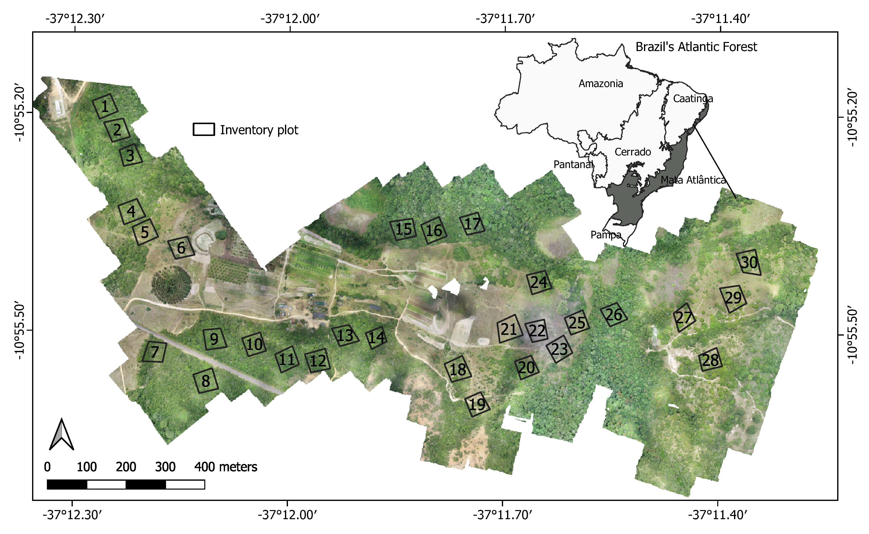
2.1. Characterization of the Study Site
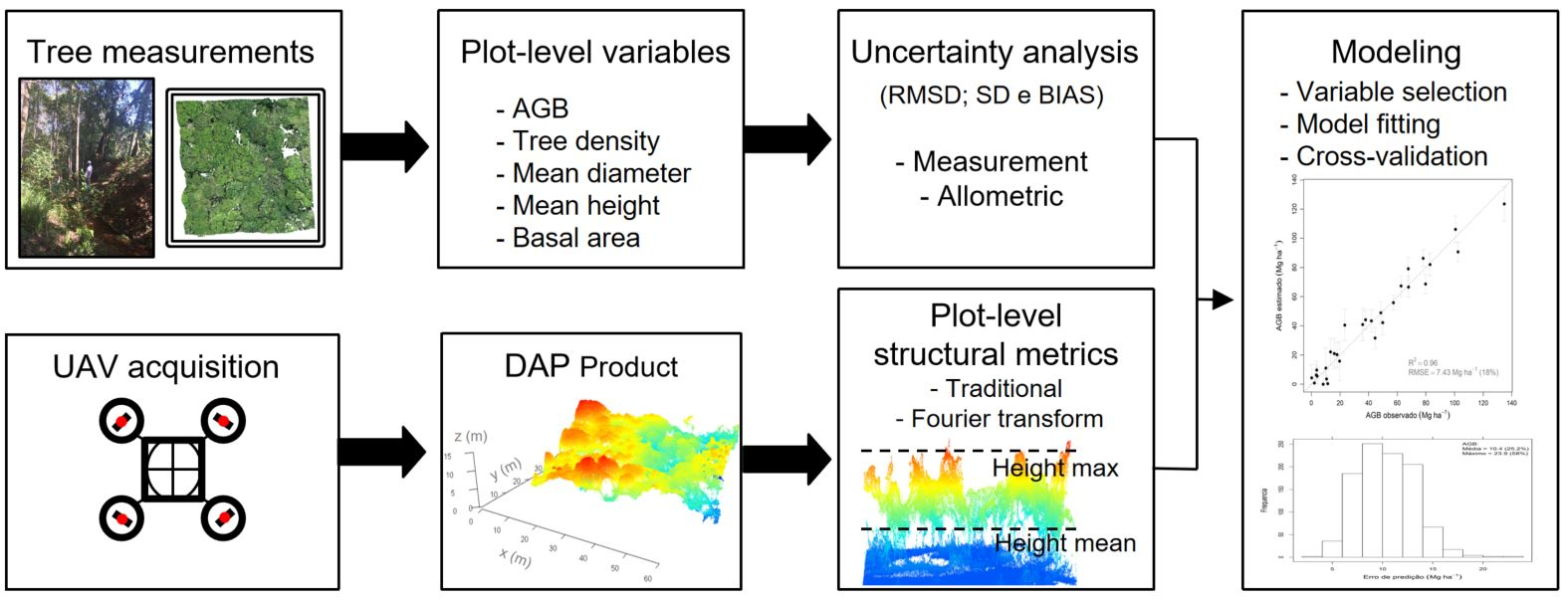
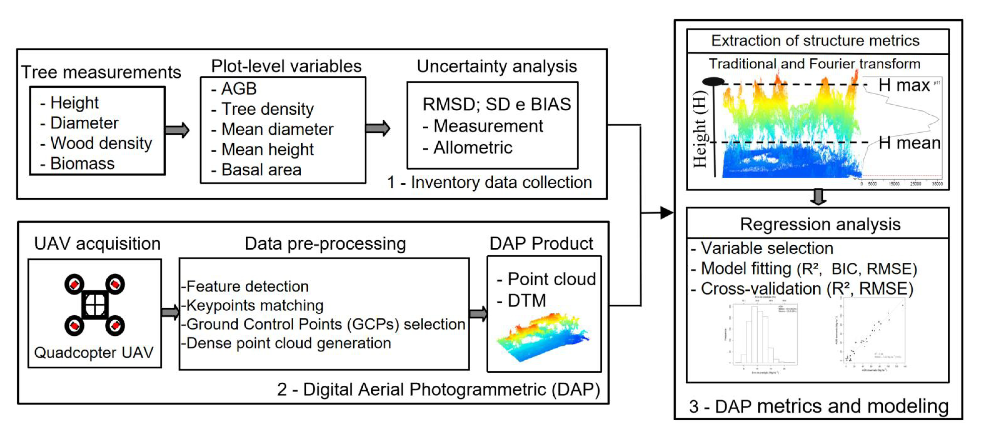
The work was carried out in a fragment of secondary tropical forest in Brazil. The fragment is located (37°11′W, 10°55′S) in an experimental farm of the Federal University of Sergipe (UFS), in the municipality of São Cristóvão, close to the Atlantic coast (Figure 1). With an area of approximately 100 ha, the forest fragment is within the Brazilian Atlantic Forest [62] and has characteristics that vary from initial secondary to late secondary forest. The major tree species found are pau-pombo (Tapirira marchandii), biriba (Eschweilera ovata), camboatá (Cupana vernalis), louro (Laurus nobilis) and amescla (Protium heptaphyllum). Overall, the forest canopy has many openings. In the study area, it was observed several types of disturbances, such as selective logging of trees, scars from forest fires, and areas of conversion to agricultural crops.
The climate classification of the area is As’ [63], being a humid tropical climate with a dry period in the summer (October to March) and rainy winter (April to September), with a total annual rainfall of approximately 1200 mm. The predominant soil is classified as red yellow argisol (EMBRAPA, 1999). The relief is smooth, with altitude values varying between 14 and 57 m and an average slope of 6%.

2.2. Methods

To assess the potential of DAP to estimate AGB in a secondary fragment of the Atlantic Forest, we followed a structured sequence of steps, which is presented in detail in Figure 2. Initially (step 1), a field campaign was carried out to measure the diameter at breast height and the height of the trees in 30 permanent forest inventory plots (∼0.25 ha). The AGB values per plot were estimated using allometric equations from the literature, and the uncertainties associated with the estimates were calculated and propagated. Simultaneous to the forest inventory, images were collected using a UAV with a multi-engine platform (step 2). The images were processed and the 3D point cloud and DTM were generated for the entire study area. After normalizing the point cloud with the DTM, vertical profiles of the forest were synthesized for each plot, and structural metrics were extracted from them. With the AGB values estimated in the field and the structural metrics derived by DAP, multiple linear regression models were adjusted and validated for the prediction of AGB and other dendrometric variables (step 3). Each step is explained in more detail the sessions below.

2.2.1. Collection of Forest Inventory Data

The field inventory was carried out between August and October 2018, in the beginning of the dry season, using a random sampling process with fixed area plots. Thirty permanent square plots with approximate dimensions of 50 m × 50 m (∼0.25 ha) were allocated. The location of these plots was previously planned to cover all the variation in biomass existing in the study area Figure 1. The four vertices of the plots were georeferenced (UTM-24S, SIRGAS 2000) with a GNSS receiver model FOIF A60 (www.foif.com), resulting in a medium horizontal (X and Y) error of 0.92 m. In the younger plots, where the height of the trees was less than three meters, or in plots with clearings located near the corners, the X, Y, and Z coordinates of the vertices were collected with GNSS in real-time kinematic (RTK) mode. In plots where it was not possible to use the RTK mode, the coordinates of the vertices were collected with GNSS in the differential, post-processed mode. The collection time of the coordinates of each vertex in the differential mode was five minutes.
The circumference of the trunk of each tree in the plot was obtained with a tape measure at the height of 1.30 m above the ground level. The circumference was converted into diameter at breast height (D). In plots in an advanced successional stages, all individuals above 5 cm D were measured. In the initial-stage plots, in addition to individuals over 5 cm, the number of individuals with D between 2 and 5 cm was counted. The total height values ( H o b s ) of the trees were estimated visually by a trained observer.
Before the beginning of the inventory of each plot, five height estimates of the trees were performed with the aid of a Haglöf electronic clinometer ( H c o r ) (http://www.haglofsweden.com), resulting in a total resampling effort of 2%. The trees were chosen at random in an attempt to cover all height variation in the plot. Following the methods of Gonçalves [46], these heights were used to correct the observer’s height estimates ( H o b s ) using a linear regression model adjusted between the two observations ( H c o r × H o b s ). While ideally clinometer measurements could be taken for all sampled trees, in practice this approach is time-consuming and not cost effective. The method used here offered a convenient alternative that can produce accurate results [46].
In the trees selected for height measurement with the aid of a clinometer, the D values were also remeasured to estimate the measurement error. Tree-level data were used to calculate the following plot-level variables: biomass (AGB), number of individuals per ha 1 (N), mean diameter at breast height ( D p l o t ), mean height ( H p l o t ), and basal area (BA). D p l o t and H p l o t values were estimated by the arithmetic mean of all individuals in the plot.

2.2.2. Estimation of Biomass and the Associated Uncertainty

The biomass (M) value of each live tree ( M t r e e , kg) was estimated using a general tropical allometric equation (Equation (1), Table 1) based on measurements of D, H c o r , and wood density ( ρ ) [64]. The wood density of each species identified in the plot was obtained in the literature [65] at the species or genus level. The biomass of the identified palm species was estimated based on Equation (2) in Saldarriaga et al. [66]. In plots in initial stage of development, in addition to the D measurements of trees above 5 cm, the number of individuals with D between 2 and 5 cm was counted. For these plots, the M t r e e values for individuals with D between 2 and 5 cm were estimated considering the center of the diameter class (3.5 cm), the fixed height of two meters, and the average wood density value of the plot. Two meters was the average height value estimated for individuals with D between 2 and 5 cm. The biomass value found was multiplied by the number of individuals in the plot. After estimating the individual biomass of each tree, the values were added and divided by the plot area, resulting in an estimate of the AGB values per hectare (Mg ha 1 ).
In most studies of AGB estimation using 3D remote sensing data, the biomass values in the field are estimated by allometric Equations (3)–(6) available in the literature [67,68,69,70]. As a result, the final model fit with remote sensing data provides an estimate of the AGB performed by the allometric equations. In this study, the uncertainties in the field biomass were estimated and propagated to the final models based on the study of Goncalves et al. [71].
With the measured values of tree diameter and height (Section 2.2.1), measurement errors were described in total, systematic, and random terms [71]. The total error was quantified by the root-mean-square deviation (RMSD), while the systematic and the random errors were quantified by the Bias and the standard deviation (SD) of the measurement differences e i , respectively
R M S D = 1 n i = 1 n ( e i ) 2 , with e i = ( m 1 i m 2 i )
B i a s = 1 n i = 1 n e i
S D = 1 n 1 i = 1 n ( e i M e a n ) 2 ,
where “n” is the number of pairs of repeated measurements for D and H c o r ; m 1 i = the first measurement of D or H c o r ; and m 2 i = the second measurement of D or H c o r .
The error in the wood density values was obtained in the literature [65]. The measurement errors in diameter at breast height ( σ D ), height ( σ H c o r r ), and wood density ( σ ρ ) were propagated to the allometrically estimated biomass by expanding the equations in Table 1 M t r e e 1 with the Taylor series and maintaining only first order terms. For a biomass model of the type M t r e e 1 = aD K H c o r ρ , with ρ not correlated with D and H c o r , the uncertainty in the biomass estimate of each live tree ( σ M ) was estimated in terms of measurement errors by [64]
σ M = M t r e e k 2 σ D 2 D 2 + σ H c o r 2 H c o r 2 + σ ρ 2 ρ 2 + 2 k σ D H 2 D H 1 / 2 ,
where “k” = 2, and DH is the covariance between D and H c o r .
The uncertainty of the allometric model was estimated in terms of the model selection error ( σ s ) and the residuals of the selected model ( σ A ). The σ s was calculated by the standard deviation of the biomass values of each tree estimated by the original equation ( M t r e e 1 ) and by the four alternative equations shown in Table 1 ( M t r e e 2 , M t r e e 3 , M t r e e 4 , M t r e e 5 ). The σ A was estimated by the equation [64,72,73]
σ A = C F 2 1 A G B ,
where “CF” is the correction factor.
The σ M , σ S , and σ A errors were calculated at the tree level and added in quadrature to obtain plot-level estimates on a per-hectare basis. These plot-level errors, in turn, were combined in quadrature to obtain a total estimate of uncertainty σ A G B under the premises of additivity and statistical independence [71].

2.2.3. Digital Aerial Photogrammetry (DAP)

UAV Data

High spatial resolution images were acquired by a DJI Phantom 4 PRO (SZ DJI Technology Co., Ltd., Shenzhen, China) quadcopter UAV platform on 27 September 2018. The climatic conditions were clear sky and moderate winds (<10 m s 1 ). Two flights were made with intersection areas to cover the entire area of interest. With a single charge, the average flight time was 14 min and covered an area of about 50 ha. The flights were conducted by the operator using the visual line of sight (VLOS) method at 120 m above ground level (AGL), following the Brazilian UAV piloting standards (https://publicacoes.decea.gov.br). The parameters for each flight and the sensor are shown in Table 2.

Photogrammetric Processing of UAV Imagery
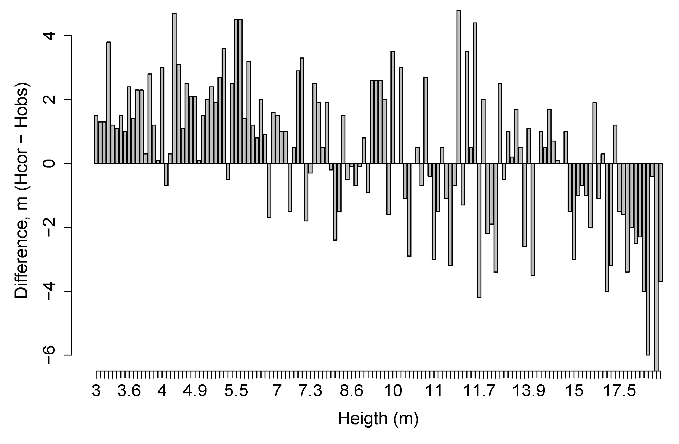
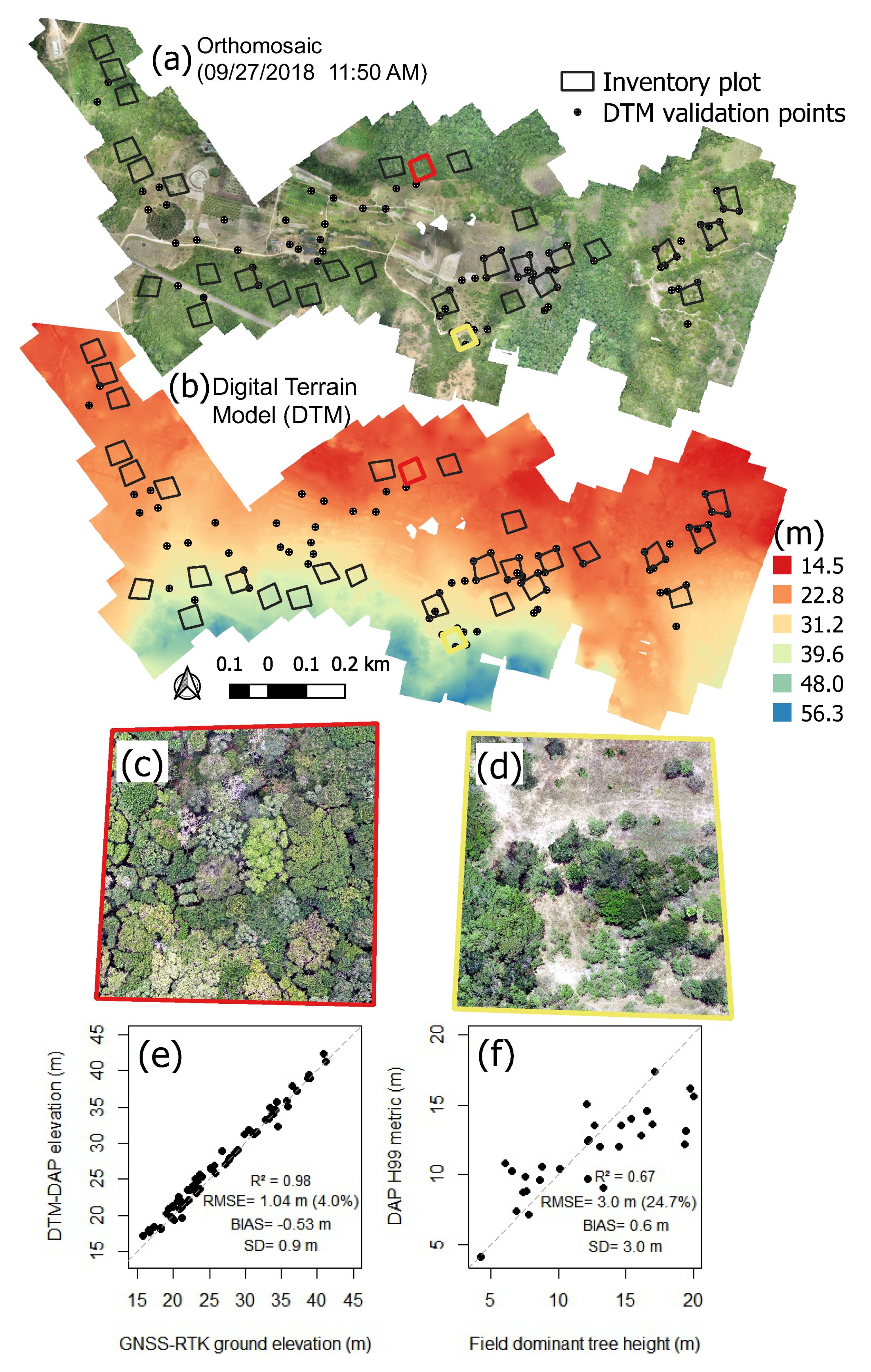
The photogrammetric processing software Agisoft Metashape Professional Edition 1.6 [74] (www.agisoft.com) was used to generate the DTM and the 3D point clouds. The software offers a combination of structure-from-motion (SfM) algorithms [22,75] used to align the camera, find the homologous points in the overlapping images, and perform the reconstruction of the 3D geometry [76] (Table 3).
An intermediate process was used to optimize the positioning and alignment of the cameras, allowing a more precise construction of the 3D model, as performed by Domingo et al. [77]. For georeferencing the images, 41 three-dimensional ground control points (GCPs) were randomly distributed across the study area, 31 of which were used as control and ten as checkpoints. The coordinates of the GCPs were collected by a GNSS receiver model FOIF A60 (http://www.foif.com) in RTK mode, with a horizontal accuracy of ±0.007 m and a vertical accuracy of ±0.011 m. The dense cloud module was used to build the dense point clouds with the average densification quality option. At the end of the process, the horizontal and vertical root mean square error (RMSE) values, calculated with the ten checkpoints, were 0.04 and 0.11 m, respectively. Finally, the generated point clouds were exported in LAS format.
The DTM was built from the DAP point cloud using the Adaptive Triangulated Irregular Network (TIN) algorithm developed by Axelsson et al. [78], implemented in Agisoft Metashape Professional Edition 1.6 [74]. In this iterative algorithm, the point cloud is divided into a square grid. In each cell, the lowest point in the point cloud is detected and then triangulated to produce the first TIN. Subsequently, the grid points not used for the construction of the initial TIN are classified according to the linear distance to the nearest triangular face and the angles formed with the vertices of that triangular face. The points are classified as terrain when the distance and the angle formed are less than that established by the user. This process is repeated until there are no more points to be checked. We used a cell size of 50 m, a linear distance of 1 m, and an angle of 15°. In a study that evaluated the impact of different values of horizontal distance and angle on the generation of DTM from DAP point clouds obtained in a tropical forest area, no significant difference was observed between the generated DTMs [42].

DAP Assessment

The quality of the generated DTM was evaluated by two methods: (i) comparing the altitude values of the DTM with those measured with a GNSS at 73 points randomly distributed in the study area, and (ii) comparing the dominant height values of each plot measured in the inventory with the 99th percentile height values extracted from the 3D point clouds normalized by the DTM. Comparisons were performed using simple linear regression [79], and calculating the RMSE, the systematic error (Bias), and the SD. The terrain altitude values were measured in the field with the GNSS in RTK mode, with an altimetric precision of ±0.02 m. The dominant height was estimated by the average of the 25 tallest trees in the plot.

2.2.4. Structural Metrics

With the normalized point clouds, traditional metrics based on height information were estimated, as were metrics based on the Fourier transform of DAP vertical vegetation profiles of each inventory plot [44,45]. The vertical profiles of each plot were generated by dividing the 3D point clouds into vertical bins of 50 cm and counting the number of points present in each bin. Traditional metrics were estimated using FUSION/LDV 3.42 (US Forest Service, Washington, DC, USA) [43]. Fourier metrics, on the other hand, were calculated with custom scripts implemented in R [80].

Traditional Metrics

Traditional canopy height metrics and metrics that represent different aspects of canopy cover were calculated from the DAP point cloud to describe the structure of each plot. The height cutoff value of 1.5 m was used as a threshold to separate points representing the ground and the understory vegetation from those associated with the trees of interest (D ≥ 5 cm). The canopy height metrics included basic distribution statistics (mean, mode, variance, maximum, percentiles, etc.) and statistics describing the shape of the point cloud height distribution (skewness, kurtosis, linear moments), while the canopy cover metrics included ratios of points above a specified height threshold to the total number of points. All metrics were extracted in the FUSION/LDV 3.42 software [43] and are described in Table 4.

Fourier Metrics

According to the work of Treuhaft et al. [44], traditional height-based metrics use only part of the structural information contained in the 3D remote sensing data. To make better use of the information contained in the DAP point clouds, we produced vertical vegetation profiles for each plot and calculated metrics based on the Fourier transform of the profiles [46]:
γ ( f ) = 0 w ( z ) e i 2 π f z d z 0 w ( z ) d z ,
where γ ( f ) is the Fourier transform of the profile at spatial frequency f and w(z) is the number of points found in the bin centered at height z.
The vertical profiles were decomposed into 30 Fourier frequencies ranging from 0.3 to 0.01 cycles/m (vertical wavelengths from 3.3 to 100 m), with a step of 0.01 cycles/m. This resulted in 30 additional metrics, which were represented by the modulus (or amplitude) of the resulting complex number (amp.01, amp.02, amp.03, …, amp.30).

2.2.5. Statistical Methods

The structural metrics obtained by DAP were related to AGB, tree density (trees/ha, N), mean height ( H p l o t ), mean diameter at breast height ( D p l o t ), and basal area (BA) using multiple linear regression models. The best subset of explanatory variables was selected with an exhaustive search of all possible combinations of variables, considering models with a maximum of six predictors. The best subset was selected based on the values of the Bayesian information criterion (BIC) and the coefficient of determination R 2 . The errors in the field biomass estimates ( σ A G B ), calculated for each of the 30 inventory plots, were used as weights in the AGB regression model estimated by weighted least squares. The errors in measuring height and diameter at breast height ( σ D and σ H c o r r ), at the plot level, were also used as weights in their respective regression models.
The normality and homoscedasticity of the residuals of the selected models were verified with the Shapiro-Wilk and Bartlett’s tests, respectively, at a significance level of 5%. The existence of multicollinearity in the models was diagnosed by the variance inflation factor (VIF). Monte Carlo cross-validation was used to evaluate the predictive ability of the selected models, using 1000 random splits of the dataset into training (80%) and validation (20%) data. The prediction error was taken as the average of the RMSE values obtained in the 1000 repetitions. All statistical analyses were performed using the software R [80].

3. Results

3.1. Forest Inventory

The differences between the tree heights (n = 150) estimated by the trigonometric (clinometer) and visual methods are presented in Figure 3. The RMSD was approximately 2.5 m, and the most significant differences were observed in the tallest trees. In general, visual height estimates of the observer were underestimated by the clinometer in trees smaller than ∼9 m and overestimated in trees larger than ∼15 m. A random behavior of the differences is also noted between the heights of 9 and 15 m. In the equation fit to correct the visually-estimated heights (H c o r = −1.1466 + H o b s ∗ 1.0792), the coefficients were significant at the 5% level, and the R 2 was 0.74. With this model, all heights estimated with the visual method in the field were corrected (H c o r ) for use in this study.
The errors calculated for the tree diameter (D) and height (H c o r ) measurements are shown in Table 5. As expected, the errors observed in the D measurements (RMSD = 2.8%) were significantly lower than those observed in the height measurements (RMSD = 24%). The systematic error was close to zero; that is, there was no trend. Regarding the wood density ( ρ ), the values obtained in the literature indicated an average error of 23%.
The secondary Atlantic Forest showed AGB values ranging from near zero to 135 Mg ha 1 (Table 6). The mean diameter ( D p l o t ) and the tree density (N) varied widely among plots. In terms of mean height, the average value observed can be considered low (∼7 m) for the type of forest analyzed, despite the high variation observed. The basal area also showed a significant variation, following the trends observed for the mean diameter.

3.2. Biomass Uncertainty

The measurement errors in diameter at breast height (2.8%), height (24.2%), and wood density (23.0%) resulted in an average error in the biomass estimate at the tree level of approximately 50% (Table 7). However, this error was reduced to 6.7% on average, when biomass was estimated at the plot level ( σ M , Table 4). The error associated with the selection of the allometric equation ranged from 0.8% to 10% and was 6.5% on average, similar to the measurement error. The error associated with the residuals of the allometric model was 2.6% on average, contributing only 16% of the total biomass variance. The total uncertainty in the plot-level biomass estimates ranged from 2.9% to 37.5%, with an average of 9.7%.

3.3. Dap Assessment

Figure 4 presents the orthomosaic (Figure 4a) and the DTM (Figure 4b) for the entire study area, and the detail of the orthomosaic for two field plots highlighted in red and yellow (Figure 4c,d). The figure also shows scatterplots for the evaluation of the accuracy based on the terrain elevation (Figure 4e) and the dominant tree height values (Figure 4f). In addition, it shows the distribution of the 73 points used for validating the elevation in the field (circles) and the limits of the 30 inventory plots. The elevation values of the DTM varied between 14.5 and 56 m and the plots were distributed over this entire interval. The elevation values collected with the GNSS in RTK mode varied between 15 and 45 m.
The RMSE found for the terrain elevation was 4.0% (1.0 m), while the RMSE obtained for the dominant tree height was significantly higher (3.0 m or 24.7%). The terrain elevations measured in the field were highly correlated with (R 2 = 0.98), and slightly overestimated by (Bias = −0.53 m) the DTM. For plots with dominant heights up to ∼12 m, the H99 metric extracted from the DAP point cloud overestimated the field height, whereas for plots with dominant heights above 12 m an opposite trend was observed (Figure 4e).
The point density of the DAP cloud was 200 pts/m 2 . In Figure 5, it is possible to observe the DAP point cloud, the DTM, and the associated elevation values extracted over the transect represented by the dotted line for two inventory plots in the study area: a plot with 1510 trees ha 1 and 78.1 Mg ha 1 (a–e); and a plot with 738 trees ha 1 and 8.2 Mg ha 1 (f–j). In general, the 3D DAP point clouds represented the structure of the top of the canopy well, regardless of the tree density. However, the DTM better represented the variation of the terrain under the canopy in the plots with lower density (red line in Figure 5h), when compared to plots with a more closed canopy (e.g., Figure 5c).

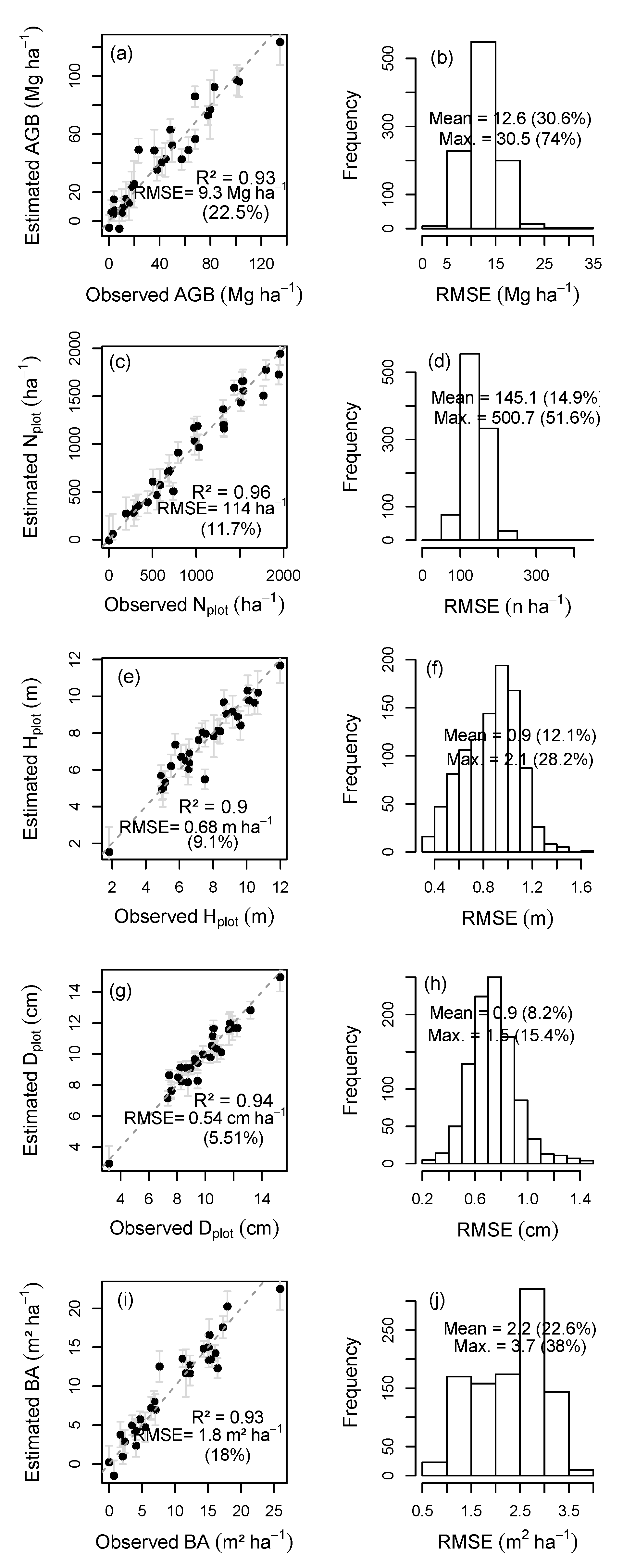
3.4. Statistical Models

The best model fit to estimate AGB showed a high performance, with a R 2 of 0.93 and a RMSE at the plot level of 9.3 Mg ha 1 (22.5%) (Table 8 and Figure 6a,b). The explanatory variables selected were the amplitude of Fourier transform at four different frequencies (amp.12, amp.13, amp.14, and amp.15), the 20th percentile of the point cloud height values (H20), and the percentage of points with height values above the mode height of the plot (CC% H m o d e ).
The model residuals showed normal distribution with constant variance, confirmed by the Shapiro-Wilk (p = 0.25) and Bartlett’s (p = 0.24) tests. Also, the existence of multicollinearity between the selected explanatory variables was not observed, as indicated by VIF values less than 10. The cross-validation process resulted in a maximum error of 30.5 Mg ha 1 (74%). However, the error was below 18.3 Mg ha 1 (44.4%) in 95% of the repetitions, with an average value of 12.6 Mg ha 1 (30.6%) (Figure 6b).
Besides AGB, it was possible to estimate the values of N, H p l o t , D p l o t , and BA with a high level of accuracy in the studied forest fragment (Table 8 and Figure 6). For all models fitted, the R 2 values were above 0.9, and the RMSE values were below 20%. In the cross-validation, the average R 2 values were above 0.84 and the RMSE was below 22.6%.
In the models selected for estimating tree density, mean diameter, and basal area, the explanatory variables selected included at least one Fourier amplitude, traditional height-based metrics, and one canopy cover metric (Table 8), as observed for the AGB model. As for the mean height model, only metrics based on the Fourier transform and height-based metrics were selected (Table 8). The normality and homoscedasticity of the residuals were confirmed by the Shapiro-Wilk and Bartlett’s tests (p > 0.05) in all models. In addition, multicollinearity issues were not observed among the selected explanatory variables (VIF < 10).

4. Discussion

4.1. Uncertainties in the Estimation of Field AGB

In a study conducted by Gonçalves et al. [71], the authors evaluated measurement, allometric, temporal, and co-location errors associated with plot-level AGB estimates produced for the calibration of remote sensing data. They found that, although small when considered individually, combined, measurement and allometric errors can result in uncertainties of up to 30%. However, these errors are usually overlooked in the analysis, which can mask the final errors found in AGB models based on remote sensing data.
In this study, the mean total error of the AGB estimates used in the calibration was approximately 10%, lower than that found in other tropical forests [44,66]. It should be noted that the equation by Chave et al. [70] was fit using data from a high number of tropical forest species, covering different classes of diameter, height, and wood density, resulting in reliable estimates of biomass and reduced errors. The measurement error ( σ M ) and the error associated with the choice of the allometric equation ( σ S ) found in this study were 6.7% and 6.5% on average, similar to those found by Gonçalves et al. [71] (6.4% and 7.1%, respectively). The error related to the residuals of the allometric model ( σ A ) was the lowest source of uncertainty, with an average of 2.6%.
The relatively low errors found in this study are also associated with the fact that we were able to overlook two common sources of uncertainty: the error resulting from spatial disagreement between field and remote sensing measurements (i.e., co-location error), and the error introduced when accounting for temporal differences in data acquisition. This is because the four vertices of the plots were georeferenced with high precision (Section 2.2.1), and the time difference between the field inventory and the remote sensing data acquisition was lower than 30 days. However, despite being small, the calculated errors were still considered in the fit of the regression models.

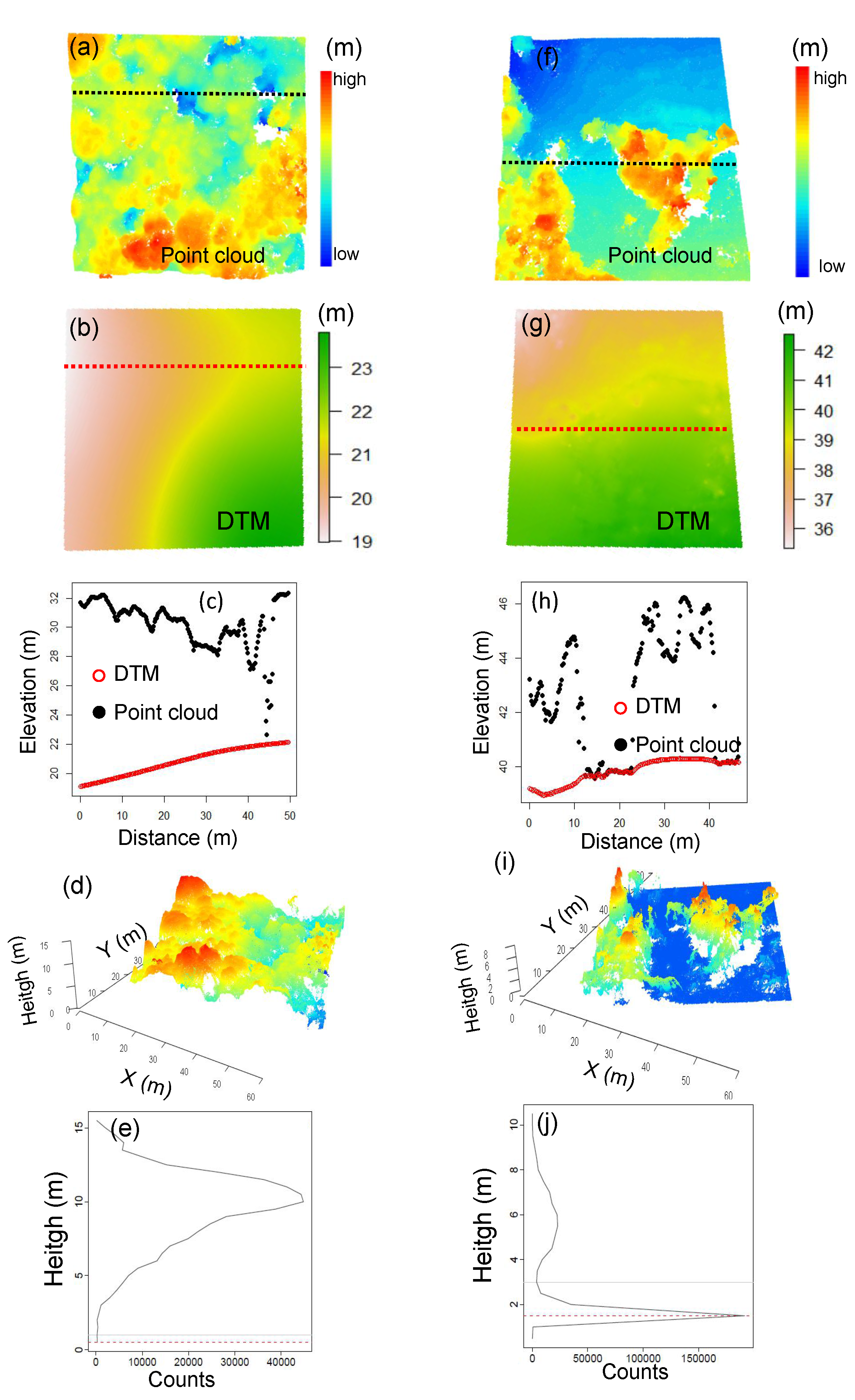
4.2. Reconstruction of the 3D Forest Structure Using DAP

The products obtained by DAP (DTM and 3D point clouds) represented well the height and the structure of the analyzed forest canopy (Figure 4 and Figure 5), as observed in other studies [29,77,79,81,82]. The results found in this work indicate that the DAP technique can be used as an alternative tool to LiDAR for the characterization of vegetation, with the advantage of presenting a lower cost in the survey of small areas. Despite fundamental differences observed between these techniques, several studies show agreement between the point clouds generated by DAP and LiDAR [41,81,83].
In this study, we chose to use GCPs to assist in the pre-processing of the aerial images and thus guarantee the best quality possible in the DAP products for the estimation of AGB at the plot level (∼0.25 ha). The low vertical RMSE (13 cm) found in the process of aligning and georeferencing the photos proves the quality of the three-dimensional information generated with this approach. However, at the scale of several hectares, it should be noted that studies such as that by Swinfield et al. [84] suggest that the use of GCPs tends not to significantly influence biomass estimates, despite its importance in applications that require a high level of spatial and temporal detail. The process of collecting these points is usually slow and expensive, and this activity may not be feasible in large forest areas. It is worth noting that the quality of the point clouds generated by DAP is also related to factors such as weather conditions, overlap rate, ground sample distance (GSD), and type of sensor used, among other characteristics [77,81,85].
The performance of DAP in forest areas is a function of the quality of the DTM used, among other factors [79]. The DTM is used to normalize the 3D point clouds (Figure 5b,g) and thus allow the characterization of the vertical structure of the vegetation. The high agreement found between the measured and estimated elevation values (RMSE = 1 m or 4%, R 2 = 0.98) (Figure 4e) prove the strong performance of the DTM generated to represent areas with a low vegetation density (Figure 5, second column), as observed by Kachamba et al. [42] in tropical dry forests (“miombo” woodlands) in northern Malawi, Africa. Despite the low error, the values found in our area were slightly overestimated (Figure 4e), as observed in other DAP studies [79,82]. In addition to the good performance of the point cloud filtering and interpolation processes used, it is worth mentioning that the studied area is quite fragmented and has a high number of clearings (Figure 4a,d), which made it possible to view the terrain at various points inside the vegetation. We note that more than 80% of the Atlantic Forest fragments are smaller than 50 ha, with the average distance between fragments being approximately 1440 m [57]. Therefore, the “patchy” conditions observed in our study area, which facilitate the construction of accurate DTMs, are characteristic of the Atlantic Forest biome. The fragment is inserted in a region with strong agricultural aptitude, bordering annual crops in proximity to roads to evacuate production. This also made it possible to visualize the terrain in areas adjacent to the forest fragment, helping the interpolation process for the generation of the DTM.
Despite the good performance of the DAP in representing the canopy of the studied forest, it is essential to highlight that the point clouds had a less satisfactory performance in representing the terrain and the understory in areas of denser vegetation cover (Figure 5, first column). This result was also found by Dandois et al. [79,82] when comparing forest and non-forest testing areas on The University of Maryland, Baltimore County campus. The use of this tool may, therefore, be impractical in certain types of vegetation, as observed by other authors in different forest formations [42,83]. Dietmaier et al. [40], for example, found that canopy openings should be at least 200 m2 in order for DAP to be able to characterize the ground response with accuracy, when working in a disturbed Boreal forest in northern Alberta, Canada.
Even explaining 67% of the variation in the dominant height values observed in the field (Figure 4f), the RMS error found in the study area was approximately 3.0 m (RMSE = 24%). However, in addition to the error associated with the H99 metric, the measurement error (2.5 m, 24.2%) found for the height of the trees (Table 5) should also be considered when assessing the quality of the DAP products generated in this study. These maximum height values extracted directly from the point cloud (H99) usually underestimate the actual height, as demonstrated in the literature review by Goodbody et al. [21]. The results found in this study confirm the above, with H99 values underestimating the dominant height in taller plots (Figure 4f). Therefore, a direct association of tree height values obtained in the field with those obtained indirectly by DAP is not recommended. Ideally, structural metrics derived from DAP should be employed in the fit of statistical models for height estimation, as demonstrated in this study.

4.3. DAP for Biomass Estimation

REDD+ mechanisms can make use of remote sensing techniques to estimate the amount of AGB in forests over time and space [2]. With the advancement of DAP techniques, point clouds obtained by UAV have also been used in AGB estimation studies [19,83]. However, few studies investigate the estimation of AGB in secondary tropical forests, and virtually no study explores the potential of DAP for the estimation of other variables of interest in these secondary forests, such as basal area, tree density, diameter and height. In the vast majority of studies based on DAP, the point cloud is normalized by a DTM obtained by LiDAR, increasing the cost of the process [29,30,31]. It is also important to highlight that, unlike most studies that use remote sensing data to fit models for estimating forest structure, in this work, measurement ( σ M ) and allometric ( σ s and σ A ) errors were taken into account. The models performed well, with errors similar in magnitude to those found in studies that did not consider the uncertainties in the field biomass [19,42], but with the advantage of using an appropriate weighted fit.
The AGB model developed presented a high R 2 value and a low RMSE (Table 8 and Figure 6). The results are similar to those found in other studies based on DAP [19,42] and reinforce the potential of products derived by DAP for biomass inventory. The structural metrics selected in the AGB model managed to explain 93% of the variation in biomass at the plot level, with performance comparable to that obtained in studies carried out with LiDAR [17,45,50,86]. The cross-validation process indicated a high predictive ability of the model, with an average RMSE of 12.60 Mg ha 1 (30.6%). This result was better than that observed by Domingo et al. [77] in the estimation of AGB in a tropical woodland forest (RMSE = 31.51%), where a 10 cm ground sample distance (GSD) and a 70% overlap rate were used.
In addition to the quality of the generated DAP product, it is worth highlighting the contribution of metrics based on the Fourier transform, which were demonstrated in the context of DAP profiles for the first time in the present study. In the model selected for the estimation of AGB, four amplitudes of the Fourier transform were included, calculated at spatial frequencies ranging from 0.12 to 0.15 cyc/m (amp.12, amp.13, amp.14 and amp.15). Qualitatively, the selection of these metrics suggests that the biomass in the study site has a strong dependence on variations in the forest structure observed in vertical scales ranging from 6.7 to 8.3 m (vertical wavelength = 1 / frequency). As in the study by Treuhaft et al. [45], the vertical scales associated with the selected frequencies coincide with the average height of the plots, as measured in the field. The use of the Fourier transform makes it possible to explore finer details in the vertical structure, which in general are omitted in traditional height-based metrics [45,46].
In addition to Fourier metrics, the model included two traditional metrics, calculated directly from the point clouds: the relative height associated with the 20th percentile (H20) and a canopy cover metric, calculated as the percentage of points in the DAP cloud with height above the mode height (CC%H m o d e ). This result suggests that optimal models for the prediction of biomass include a combination of metrics that capture the vertical structure with metrics that describe the canopy cover.
It should be noted that the metrics selected in this study may not be suitable for estimating biomass in forests with different structures. The low density of individuals, the large number of clearings, and the existence of roads and temporary crops close to the analyzed fragment favored the identification of areas with soil response exposed in the images collected by UAV. After identifying the soil, it was possible to create an excellent DTM, even under the densest vegetation (Figure 5b). The normalization of the point clouds, performed by subtracting the DTM, is a fundamental process in the extraction of structural metrics to describe the forest structure [87,88]. Another fact that should be pointed out is the presence of a relatively flat terrain in the study area, which facilitated the process of interpolation of the DTM in places where it was not possible to obtain elevation values from the ground (Figure 4 and Figure 5b).

4.4. DAP for Estimation of Basal Area, Diameter, Height and Density

Traditionally, forest inventory campaigns are used to define the best vegetation management strategy and formulate effective forest policies [89]. The high cost, the complexity of the survey, and the impact of climate change on forests have motivated the modernization of campaigns and inventory methods [21,43,90]. Several studies have pointed out DAP as an alternative technique to estimate dendrometric parameters of vegetation [28,91,92,93]. In this study, the 3D DAP point cloud showed great potential for the estimation of basal area, tree density, mean height and mean diameter at breast height at the plot level (Table 8 and Figure 6). The best result obtained was in the prediction of mean diameter values, with an average RMSE in the cross-validation process of 0.8 cm (8.2%). This error was lower than that found by Nurminen et al. [94] (RMSE = ∼12%) in a study that tested two different rates of overlap in image acquisition in a forest in Sonkajärvi, in central Finland. Mean height was estimated in this study with a RMSE of 0.9 m (12.0%), slightly higher than the error found by Navarro et al. [92] (RMSE = 1.58 m or 10.71%) in the estimation of height in a managed pine forest located in the north of Madrid, Spain. Ota et al. [95] managed to explain 93% of the height variation in a temperate coniferous forest, with a cross-validation error of approximately 7%. Krause et al. [96] also obtained excellent results in estimating individual tree heights, with a RMSE below 0.5 m. It should be noted that in all studies mentioned above, the DTM was obtained using LiDAR techniques, which is different from the technique used in this study. The model for estimating the number of individuals per hectare explained 94% of the variation, with a RMSE of 145.1 ha 1 (∼15%), also yielding satisfactory results when compared to similar studies [92]. The basal area was also estimated with a good performance when compared to other studies, despite showing the highest errors among all variables analyzed (RMSE = 2.2 m 2 ha 1 or 22.6%). Straub et al. [97], for example, found errors close to 30% when estimating basal area in mixed forests in Europe.
As in the AGB model, the amplitude of the Fourier transform was selected in at least one frequency in all models described above. In the predictive models of tree density and mean diameter, the frequency of 0.06 cyc/m (amp.06) was selected, corresponding to a vertical wavelength of 16.7 m. In the basal area model, the frequency of 0.21 cyc/m (amp.21) was selected, corresponding to a vertical scale of 4.8 m, and in the mean height model, two frequencies (amp.06 and amp.25) were selected, corresponding to vertical scales of 16.7 and 4 m, respectively. These results reinforce the importance of exploring finer details of the vertical forest structure when developing predictive models for inventory attributes.
In addition to the metrics based on the Fourier transform, all models included conventional height-based and/or canopy cover metrics, following the pattern observed in the AGB model. For the tree density model, a traditional metric (Table 8) that describes the structure of the canopy (CC%H m e a n ) was selected, exploring the close relationship between number of trees and canopy cover. A measure of dispersion of height values (H s k e w ) was also selected, in addition to three statistics related to the height distribution in the plot (HMAD M o d e , H60, and HCRR). For the height model, traditional metrics were selected that describe the dispersion of height values in the plot (HL k u r t ) and three relative heights associated with the first (H01), fifth (H05), and tenth (H10) percentiles. For the mean diameter model, only measures that describe the position of the heights were selected, including measures based on the calculation of moments (HL3, HL4, and HL s k e w ), the height corresponding to the first percentile (H01) and the fraction of points with height above the mean height of the plot (CC%H m e a n ). Finally, in the basal area model, two variables related to measurements of central tendency (H m e a n and H50) and a canopy cover measure (CC%H m e a n ) were selected. All models, except the height model, included a canopy cover metric as an explanatory variable. Cover metrics contain information on the horizontal structure of the forest, which is not relevant for height estimation. We highlight the CC%H m e a n metric, which was selected in the models for N, D p l o t , and BA, representing an important structural measure for the estimation of dendrometric variables in the analyzed forest.

5. Conclusions

Digital aerial photogrammetry (DAP) techniques were used to estimate aboveground biomass (AGB), tree density (N), mean diameter at breast height ( D p l o t ), mean height ( H p l o t ), and basal area (BA) in a fragment of secondary Brazilian Atlantic Forest in northeastern Brazil. Decision making based on forest inventory must consider the interactions between forest growth and climate in a climate change scenario. Mapping and accurate estimation of AGB and other dendrometric variables may allow for more versatile planning to minimize carbon emissions, preserve biodiversity, and detect forest degradation processes early.
The results of this study indicate that products derived from DAP, produced without the support of auxiliary data, can be used for the calibration of useful models for estimation of AGB and other forest variables of interest in secondary forest fragments of the Atlantic Forest, supporting the implementation and monitoring of REDD+ projects. The results also demonstrate the potential use of DAP in operational forest inventory to enable quick access to information by forest managers. We conclude that the uncertainties associated with field estimates of biomass using allometric equations provided in the literature should be taken into account in the statistical modeling, providing more reliability in the final results. We also conclude that techniques that make it possible to explore finer details of the forest structure captured by point clouds, such as the Fourier transform of vertical profiles, provide a significant gain in accuracy, especially when combined with traditional metrics that describe canopy cover.
Further studies should be carried out to evaluate the effects of different rates of overlap and flight height, processing parameters, as well as the need to use control points. In addition, studies must be carried out in an area with sloping terrain, which can impair the construction of the DTM. Future studies should also assess the contribution of spectral data to structure-based models to improve forest inventory estimates derived from DAP.

Author Contributions

A.A. conceived, designed, and performed the experiment; analyzed the data; and wrote the paper. F.G. assisted with study design, data analysis and writing of the paper. G.S., R.S. and R.T. assisted with interpretation of results, and writing of the paper. W.S. assisted with data collection and contributed to parts of the analysis. D.L. and M.F. assisted with data collection and writing of the paper. All authors have read and agreed to the published version of the manuscript.

Funding

This research was funded by CNPq grant number 427143/2016-0 and 310299/2019-5.

Acknowledgments

The authors would like to thank CNPq for the financial support of the project “Monitoring the quality and quantity of water in a hydrographic basin in the coastal tray of northeastern Brazil” (427143/2016-0) and the research grant from the first author of the project “Models for estimating biomass and other dendrometric characteristics of a secondary forest” process 310299/2019-5”. Also thank the Rural Campus of the Federal University of Sergipe (UFS), for the logistical support during the fieldwork and Marcolino for the special support at field work. A portion of this research was carried out at the Jet Propulsion Laboratory, California Institute of Technology, under a contract with the National Aeronautics and Space Administration (80NM0018D0004). The authors would also like to thank the Terrestrial Ecology Program (https://cce.nasa.gov/terrestrial_ecology/).

Conflicts of Interest

The authors declare no conflict of interest.

Abbreviations

The following abbreviations are used in this manuscript:
3DThree dimensions
AGBAboveground Biomass
AGLAbove Ground Level
ampFourier amplitude
BABasal area
BICBayesian Information Criterion
CFCorrection Factor
DDiameter at breast height
DAPDigital Aerial Photogrammetry
D p l o t Mean plot diameter
DTMDigital Terrain Model
EMBRAPABrazilian Agricultural Research Corporation
GCPsGround Control Points
GNSSGlobal Navigation Satellite System
HTree height
H c o r Corrected tree height
H o b s Visually estimated tree height
H p l o t Mean plot height
IPCCIntergovernmental Panel on Climate Change
InSARInterferometric Synthetic Aperture Radar
LiDARLight Detection and Ranging
m 1 First measurement D or Hobs
m 2 Second measurement D or Hobs
M p a l m Dry aboveground biomass of palm species
M t r e e Dry aboveground biomass of tree species
NNumber of trees per hectare
REDD+Reducing Emissions from Deforestation and Forest Degradation
RMSDRoot Mean Square Deviation
RMSERoot Mean Square Error
RTKReal-Time Kinematic
SDStandard Deviation
SfMStructure from Motion
SIRGASGeocentric Reference System for the Americas
UAVUnmanned Aerial Vehicle
UFSFederal University of Sergipe
UTMUniversal Transverse Mercator
VLOSVisual Line of Sight
w(z)The number of points found in the bin centered at height z
XX coordinate
YY coordinate
γ ( f ) Fourier transform
ZZ coordinate
σ A Uncertainty associated with the residuals of the allometric model
σ A G B Total uncertainty of the AGB estimate
σ D Measurement errors in diameter at breast height
σ H Measurement errors in tree height
σ M Uncertainty in the biomass estimate of each tree
σ ρ Measurement error in wood density
σ S Uncertainty associated with the allometric model selection
ρ Wood density

References

  1. Andersen, H.E.; Reutebuch, S.E.; McGaughey, R.J. A rigorous assessment of tree height measurements obtained using airborne lidar and conventional field methods. Can. J. Remote Sens. 2006, 32, 355–366. [Google Scholar] [CrossRef]
  2. Houghton, R.; Greenglass, N.; Baccini, A.; Cattaneo, A.; Goetz, S.; Kellndorfer, J.; Laporte, N.; Walker, W. The role of science in Reducing Emissions from Deforestation and Forest Degradation (REDD). Carbon Manag. 2010, 1, 253–259. [Google Scholar] [CrossRef]
  3. Boisvenue, C.; Running, S.W. Impacts of climate change on natural forest productivity - evidence since the middle of the 20th century. Glob. Chang. Biol. 2006, 12, 862–882. [Google Scholar] [CrossRef]
  4. Noss, R.F. Beyond Kyoto: Forest Management in a Time of Rapid Climate Change. Conserv. Biol. 2001, 15, 578–590. [Google Scholar] [CrossRef]
  5. Stas, S. Above-Ground Biomass and Carbon Stocks in a Secondary Forest in Comparison with Adjacent Primary Forest on Limestone in Seram, the Moluccas, Indonesia; Working Paper 145; CIFOR: Bogor, Indonesia, 2014. [Google Scholar] [CrossRef] [Green Version]
  6. Houghton, R.A.; Hall, F.; Goetz, S.J. Importance of biomass in the global carbon cycle. J. Geophys. Res. Biogeosci. 2009, 114. [Google Scholar] [CrossRef]
  7. IPCC. IPCC—Task Force on National Greenhouse Gas Inventories; IPCC: Hong Kong, China, 2006.
  8. Foody, G.M. Remote sensing of tropical forest environments: Towards the monitoring of environmental resources for sustainable development. Int. J. Remote Sens. 2003, 24. [Google Scholar] [CrossRef]
  9. McRoberts, R.; Tomppo, E. Remote sensing support for national forest inventories. Remote Sens. Environ. 2007, 110, 412–419. [Google Scholar] [CrossRef]
  10. Su, Y.; Guo, Q.; Xue, B.; Hu, T.; Alvarez, O.; Tao, S.; Fang, J. Spatial distribution of forest aboveground biomass in China: Estimation through combination of spaceborne lidar, optical imagery, and forest inventory data. Remote Sens. Environ. 2016, 173, 187–199. [Google Scholar] [CrossRef] [Green Version]
  11. Dube, T.; Mutanga, O. Evaluating the utility of the medium-spatial resolution Landsat 8 multispectral sensor in quantifying aboveground biomass in uMgeni catchment, South Africa. ISPRS J. Photogramm. Remote Sens. 2015, 101, 36–46. [Google Scholar] [CrossRef]
  12. Pandit, S.; Tsuyuki, S.; Dube, T. Landscape-Scale Aboveground Biomass Estimation in Buffer Zone Community Forests of Central Nepal: Coupling In Situ Measurements with Landsat 8 Satellite Data. Remote Sens. 2018, 10, 1848. [Google Scholar] [CrossRef] [Green Version]
  13. Wulder, M.; Skakun, R.; Kurz, W.; White, J. Estimating time since forest harvest using segmented Landsat ETM+ imagery. Remote Sens. Environ. 2004, 93, 179–187. [Google Scholar] [CrossRef]
  14. Nguyen, T.H.; Jones, S.D.; Soto-Berelov, M.; Haywood, A.; Hislop, S. Monitoring aboveground forest biomass dynamics over three decades using Landsat time-series and single-date inventory data. Int. J. Appl. Earth Obs. Geoinf. 2020, 84, 101952. [Google Scholar] [CrossRef]
  15. Rana, P.; Korhonen, L.; Gautam, B.; Tokola, T. Effect of field plot location on estimating tropical forest above-ground biomass in Nepal using airborne laser scanning data. ISPRS J. Photogramm. Remote Sens. 2014, 94, 55–62. [Google Scholar] [CrossRef]
  16. Clark, M.L.; Roberts, D.A.; Ewel, J.J.; Clark, D.B. Estimation of tropical rain forest aboveground biomass with small-footprint lidar and hyperspectral sensors. Remote Sens. Environ. 2011, 115, 2931–2942. [Google Scholar] [CrossRef]
  17. Margolis, H.A.; Nelson, R.F.; Montesano, P.M.; Beaudoin, A.; Sun, G.; Andersen, H.E.; Wulder, M.A. Combining satellite lidar, airborne lidar, and ground plots to estimate the amount and distribution of aboveground biomass in the boreal forest of North America. Can. J. For. Res. 2015, 45, 838–855. [Google Scholar] [CrossRef] [Green Version]
  18. González-Ferreiro, E.; Diéguez-Aranda, U.; Miranda, D. Estimation of stand variables in Pinus radiata D. Don plantations using different LiDAR pulse densities. For. Int. J. For. Res. 2012, 85, 281–292. [Google Scholar] [CrossRef]
  19. Kachamba, D.; Ørka, H.; Næsset, E.; Eid, T.; Gobakken, T. Influence of Plot Size on Efficiency of Biomass Estimates in Inventories of Dry Tropical Forests Assisted by Photogrammetric Data from an Unmanned Aircraft System. Remote Sens. 2017, 9, 610. [Google Scholar] [CrossRef] [Green Version]
  20. Zarco-Tejada, P.; Diaz-Varela, R.; Angileri, V.; Loudjani, P. Tree height quantification using very high resolution imagery acquired from an unmanned aerial vehicle (UAV) and automatic 3D photo-reconstruction methods. Eur. J. Agron. 2014, 55, 89–99. [Google Scholar] [CrossRef]
  21. Goodbody, T.R.H.; Coops, N.C.; White, J.C. Digital Aerial Photogrammetry for Updating Area-Based Forest Inventories: A Review of Opportunities, Challenges, and Future Directions. Curr. For. Rep. 2019, 5, 55–75. [Google Scholar] [CrossRef] [Green Version]
  22. Iglhaut, J.; Cabo, C.; Puliti, S.; Piermattei, L.; O’Connor, J.; Rosette, J. Structure from Motion Photogrammetry in Forestry: A Review. Curr. For. Rep. 2019, 5, 155–168. [Google Scholar] [CrossRef] [Green Version]
  23. Díaz-Varela, R.; de la Rosa, R.; León, L.; Zarco-Tejada, P. High-Resolution Airborne UAV Imagery to Assess Olive Tree Crown Parameters Using 3D Photo Reconstruction: Application in Breeding Trials. Remote Sens. 2015, 7, 4213–4232. [Google Scholar] [CrossRef] [Green Version]
  24. Tang, L.; Shao, G. Drone remote sensing for forestry research and practices. J. For. Res. 2015, 26, 791–797. [Google Scholar] [CrossRef]
  25. Tomasi, C.; Kanade, T. Shape and motion from image streams under orthography: A factorization method. Int. J. Comput. Vis. 1992, 9, 137–154. [Google Scholar] [CrossRef]
  26. Lin, J.; Wang, M.; Ma, M.; Lin, Y. Aboveground Tree Biomass Estimation of Sparse Subalpine Coniferous Forest with UAV Oblique Photography. Remote Sens. 2018, 10, 1849. [Google Scholar] [CrossRef] [Green Version]
  27. Ota, T.; Ogawa, M.; Shimizu, K.; Kajisa, T.; Mizoue, N.; Yoshida, S.; Takao, G.; Hirata, Y.; Furuya, N.; Sano, T.; et al. Aboveground Biomass Estimation Using Structure from Motion Approach with Aerial Photographs in a Seasonal Tropical Forest. Forests 2015, 6, 3882–3898. [Google Scholar] [CrossRef] [Green Version]
  28. Puliti, S.; Ørka, H.; Gobakken, T.; Næsset, E. Inventory of Small Forest Areas Using an Unmanned Aerial System. Remote Sens. 2015, 7, 9632–9654. [Google Scholar] [CrossRef] [Green Version]
  29. Shen, X.; Cao, L.; Yang, B.; Xu, Z.; Wang, G. Estimation of Forest Structural Attributes Using Spectral Indices and Point Clouds from UAS-Based Multispectral and RGB Imageries. Remote Sens. 2019, 11, 800. [Google Scholar] [CrossRef] [Green Version]
  30. Fankhauser, K.; Strigul, N.; Gatziolis, D. Augmentation of Traditional Forest Inventory and Airborne Laser Scanning with Unmanned Aerial Systems and Photogrammetry for Forest Monitoring. Remote Sens. 2018, 10, 1562. [Google Scholar] [CrossRef] [Green Version]
  31. Baltsavias, E.P. A comparison between photogrammetry and laser scanning. ISPRS J. Photogramm. Remote Sens. 1999, 54, 83–94. [Google Scholar] [CrossRef]
  32. Gobakken, T.; Bollandsås, O.M.; Næsset, E. Comparing biophysical forest characteristics estimated from photogrammetric matching of aerial images and airborne laser scanning data. Scand. J. For. Res. 2014, 30, 73–86. [Google Scholar] [CrossRef]
  33. Cao, L.; Liu, H.; Fu, X.; Zhang, Z.; Shen, X.; Ruan, H. Comparison of UAV LiDAR and Digital Aerial Photogrammetry Point Clouds for Estimating Forest Structural Attributes in Subtropical Planted Forests. Forests 2019, 10, 145. [Google Scholar] [CrossRef] [Green Version]
  34. Puliti, S.; Solberg, S.; Granhus, A. Use of UAV Photogrammetric Data for Estimation of Biophysical Properties in Forest Stands Under Regeneration. Remote Sens. 2019, 11, 233. [Google Scholar] [CrossRef] [Green Version]
  35. Goodbody, T.R.H.; Coops, N.C.; Tompalski, P.; Crawford, P.; Day, K.J.K. Updating residual stem volume estimates using ALS- and UAV-acquired stereo-photogrammetric point clouds. Int. J. Remote Sens. 2016, 38, 2938–2953. [Google Scholar] [CrossRef]
  36. Hobi, M.L.; Ginzler, C.; Commarmot, B.; Bugmann, H. Gap pattern of the largest primeval beech forest of Europe revealed by remote sensing. Ecosphere 2015, 6, art76. [Google Scholar] [CrossRef] [Green Version]
  37. Wang, Z.; Ginzler, C.; Waser, L.T. A novel method to assess short-term forest cover changes based on digital surface models from image-based point clouds. For. Int. J. For. Res. 2015, 88, 429–440. [Google Scholar] [CrossRef] [Green Version]
  38. Zielewska-Büttner, K.; Adler, P.; Ehmann, M.; Braunisch, V. Automated Detection of Forest Gaps in Spruce Dominated Stands Using Canopy Height Models Derived from Stereo Aerial Imagery. Remote Sens. 2016, 8, 175. [Google Scholar] [CrossRef] [Green Version]
  39. White, J.C.; Tompalski, P.; Coops, N.C.; Wulder, M.A. Comparison of airborne laser scanning and digital stereo imagery for characterizing forest canopy gaps in coastal temperate rainforests. Remote Sens. Environ. 2018, 208, 1–14. [Google Scholar] [CrossRef]
  40. Dietmaier, A.; McDermid, G.J.; Rahman, M.M.; Linke, J.; Ludwig, R. Comparison of LiDAR and Digital Aerial Photogrammetry for Characterizing Canopy Openings in the Boreal Forest of Northern Alberta. Remote Sens. 2019, 11, 1919. [Google Scholar] [CrossRef] [Green Version]
  41. Zahawi, R.A.; Dandois, J.P.; Holl, K.D.; Nadwodny, D.; Reid, J.L.; Ellis, E.C. Using lightweight unmanned aerial vehicles to monitor tropical forest recovery. Biol. Conserv. 2015, 186, 287–295. [Google Scholar] [CrossRef] [Green Version]
  42. Kachamba, D.; Ørka, H.; Gobakken, T.; Eid, T.; Mwase, W. Biomass Estimation Using 3D Data from Unmanned Aerial Vehicle Imagery in a Tropical Woodland. Remote Sens. 2016, 8, 968. [Google Scholar] [CrossRef] [Green Version]
  43. McGaughey, R.J. FUSION/LDV: Software for LiDAR Data Analysis and Visualization; Version 3.30; U.S. Department of Agriculture Forest Service, Pacific Northwest Research Station, University of Washington: Seattle, WA, USA, 2018; Available online: http://forsys.cfr.washington.edu/fusion/fusionlatest.html (accessed on 13 February 2019).
  44. Treuhaft, R.N.; Chapman, B.D.; dos Santos, J.R.; Gonçalves, F.G.; Dutra, L.V.; Graça, P.M.L.A.; Drake, J.B. Vegetation profiles in tropical forests from multibaseline interferometric synthetic aperture radar, field, and lidar measurements. J. Geophys. Res. 2009, 114. [Google Scholar] [CrossRef] [Green Version]
  45. Treuhaft, R.N.; Gonçalves, F.G.; Drake, J.B.; Chapman, B.D.; dos Santos, J.R.; Dutra, L.V.; Graça, P.M.L.A.; Purcell, G.H. Biomass estimation in a tropical wet forest using Fourier transforms of profiles from lidar or interferometric SAR. Geophys. Res. Lett. 2010, 37. [Google Scholar] [CrossRef] [Green Version]
  46. Aes Gonçalves, F.G. Vertical Structure and Aboveground Biomass of Tropical Forests from Lidar Remote Sensing. Ph.D. Thesis, Oregon State University, Corvallis, OR, USA, 2014. [Google Scholar]
  47. Chazdon, R.L.; Broadbent, E.N.; Rozendaal, D.M.A.; Bongers, F.; Zambrano, A.M.A.; Aide, T.M.; Balvanera, P.; Becknell, J.M.; Boukili, V.; Brancalion, P.H.S.; et al. Carbon sequestration potential of second-growth forest regeneration in the Latin American tropics. Sci. Adv. 2016, 2, e1501639. [Google Scholar] [CrossRef] [PubMed] [Green Version]
  48. Silveira, E.M.; Cunha, L.I.F.; Galvão, L.S.; Withey, K.D.; Júnior, F.W.A.; Scolforo, J.R.S. Modelling aboveground biomass in forest remnants of the Brazilian Atlantic Forest using remote sensing, environmental and terrain-related data. Geocarto Int. 2019, 1–18. [Google Scholar] [CrossRef]
  49. Silveira, E.M.; Silva, S.H.G.; Acerbi-Junior, F.W.; Carvalho, M.C.; Carvalho, L.M.T.; Scolforo, J.R.S.; Wulder, M.A. Object-based random forest modelling of aboveground forest biomass outperforms a pixel-based approach in a heterogeneous and mountain tropical environment. Int. J. Appl. Earth Obs. Geoinf. 2019, 78, 175–188. [Google Scholar] [CrossRef]
  50. Longo, M.; Keller, M.; dos Santos, M.N.; Leitold, V.; Pinagé, E.R.; Baccini, A.; Saatchi, S.; Nogueira, E.M.; Batistella, M.; Morton, D.C. Aboveground biomass variability across intact and degraded forests in the Brazilian Amazon. Glob. Biogeochem. Cycles 2016, 30, 1639–1660. [Google Scholar] [CrossRef] [Green Version]
  51. Santos, E.G.D.; Shimabukuro, Y.E.; Moura, Y.M.D.; Gonçalves, F.G.; Jorge, A.; Gasparini, K.A.; Arai, E.; Duarte, V.; Ometto, J.P. Multi-scale approach to estimating aboveground biomass in the Brazilian Amazon using Landsat and LiDAR data. Int. J. Remote Sens. 2019, 40, 8635–8645. [Google Scholar] [CrossRef]
  52. Lefsky, M.A.; Harding, D.J.; Keller, M.; Cohen, W.B.; Carabajal, C.C.; Espirito-Santo, F.D.B.; Hunter, M.O.; de Oliveira, R. Estimates of forest canopy height and aboveground biomass using ICESat. Geophys. Res. Lett. 2005, 32. [Google Scholar] [CrossRef] [Green Version]
  53. Lei, Y.; Treuhaft, R.; Keller, M.; dos Santos, M.; Gonçalves, F.; Neumann, M. Quantification of selective logging in tropical forest with spaceborne SAR interferometry. Remote Sens. Environ. 2018, 211, 167–183. [Google Scholar] [CrossRef]
  54. Treuhaft, R.; Lei, Y.; Gonçalves, F.; Keller, M.; Santos, J.; Neumann, M.; Almeida, A. Tropical-Forest Structure and Biomass Dynamics from TanDEM-X Radar Interferometry. Forests 2017, 8, 277. [Google Scholar] [CrossRef] [Green Version]
  55. Neeff, T.; Dutra, L.V.; dos Santos, R.; Freitas, C.d.C.; Araujo, L.S. Tropical Forest Measurement by Interferometric Height Modeling and P-Band Radar Backscatter. For. Sci. 2005, 51, 585–594. [Google Scholar] [CrossRef]
  56. da Silva, J.M.C.; Tabarelli, M. Tree species impoverishment and the future flora of the Atlantic forest of northeast Brazil. Nature 2000, 404, 72–74. [Google Scholar] [CrossRef] [PubMed]
  57. Ribeiro, M.C.; Metzger, J.P.; Martensen, A.C.; Ponzoni, F.J.; Hirota, M.M. The Brazilian Atlantic Forest: How much is left, and how is the remaining forest distributed? Implications for conservation. Biol. Conserv. 2009, 142, 1141–1153. [Google Scholar] [CrossRef]
  58. Becknell, J.M.; Keller, M.; Piotto, D.; Longo, M.; dos Santos, M.N.; Scaranello, M.A.; de Oliveira Cavalcante, R.B.; Porder, S. Landscape-scale lidar analysis of aboveground biomass distribution in secondary Brazilian Atlantic Forest. Biotropica 2018, 50, 520–530. [Google Scholar] [CrossRef]
  59. David, H.C.; de Araújo, E.J.G.; Morais, V.A.; Scolforo, J.R.S.; Marques, J.M.; Netto, S.P.; MacFarlane, D.W. Carbon stock classification for tropical forests in Brazil: Understanding the effect of stand and climate variables. For. Ecol. Manag. 2017, 404, 241–250. [Google Scholar] [CrossRef]
  60. Erb, K.H.; Kastner, T.; Plutzar, C.; Bais, A.L.S.; Carvalhais, N.; Fetzel, T.; Gingrich, S.; Haberl, H.; Lauk, C.; Niedertscheider, M.; et al. Unexpectedly large impact of forest management and grazing on global vegetation biomass. Nature 2017, 553, 73–76. [Google Scholar] [CrossRef]
  61. Millar, C.I.; Stephenson, N.L.; Stephens, S.L. Climate change and forests of the future: Managing in the face of uncertainty. Ecol. Appl. 2007, 17, 2145–2151. [Google Scholar] [CrossRef]
  62. Veloso, H.P.; Rangel-Filho, A.L.R.; Lima, J.C.A. Classificação da vegetação brasileira, adaptada a um sistema universal; IBGE: Rio de Janeiro, Brazil, 1991.
  63. Koeppen, W. Climatologia: Con un estudio de los climas de la tierra; Fondo de Cultura Económica: México City, Mexico, 1948; 478p. [Google Scholar]
  64. Chave, J.; Condit, R.; Aguilar, S.; Hernandez, A.; Lao, S.; Perez, R. Error propagation and scaling for tropical forest biomass estimates. Philos. Trans. R. Soc. London. Ser. B Biol. Sci. 2004, 359, 409–420. [Google Scholar] [CrossRef]
  65. Chave, J.; Muller-Landau, H.C.; Baker, T.R.; Easdale, T.A.; ter Steege, H.; Webb, C.O. Regional and phylogenetic variation of wood density across 2456 neotropical tree species. Ecol. Appl. 2006, 16, 2356–2367. [Google Scholar] [CrossRef] [Green Version]
  66. Saldarriaga, J.G.; West, D.C.; Tharp, M.L.; Uhl, C. Long-Term Chronosequence of Forest Succession in the Upper Rio Negro of Colombia and Venezuela. J. Ecol. 1988, 76, 938. [Google Scholar] [CrossRef]
  67. Chambers, J.Q.; dos Santos, J.; Ribeiro, R.J.; Higuchi, N. Tree damage, allometric relationships, and above-ground net primary production in central Amazon forest. For. Ecol. Manag. 2001, 152, 73–84. [Google Scholar] [CrossRef]
  68. Brown, S.; Gillespie, A.J.R.; Lugo, A.E. Biomass Estimation Methods for Tropical Forests with Applications to Forest Inventory Data. For. Sci. 1989, 35, 881–902. [Google Scholar] [CrossRef]
  69. Brown, S. Estimating Biomass and Biomass Change of Tropical Forests: A Primer; Food & Agriculture Organization: Rome, Italy, 1997; Volume 134, p. 55. [Google Scholar]
  70. Chave, J.; Andalo, C.; Brown, S.; Cairns, M.A.; Chambers, J.Q.; Eamus, D.; Fölster, H.; Fromard, F.; Higuchi, N.; Kira, T.; et al. Tree allometry and improved estimation of carbon stocks and balance in tropical forests. Oecologia 2005, 145, 87–99. [Google Scholar] [CrossRef]
  71. Gonçalves, F.; Treuhaft, R.; Law, B.; Almeida, A.; Walker, W.; Baccini, A.; dos Santos, J.; Graça, P. Estimating Aboveground Biomass in Tropical Forests: Field Methods and Error Analysis for the Calibration of Remote Sensing Observations. Remote Sens. 2017, 9, 47. [Google Scholar] [CrossRef]
  72. Chave, J.; Réjou-Méchain, M.; Búrquez, A.; Chidumayo, E.; Colgan, M.S.; Delitti, W.B.; Duque, A.; Eid, T.; Fearnside, P.M.; Goodman, R.C.; et al. Improved allometric models to estimate the aboveground biomass of tropical trees. Glob. Chang. Biol. 2014, 20, 3177–3190. [Google Scholar] [CrossRef] [PubMed]
  73. Baskerville, G.L. Use of Logarithmic Regression in the Estimation of Plant Biomass. Can. J. For. Res. 1972, 2, 49–53. [Google Scholar] [CrossRef]
  74. Agisoft LLC, S.P. Agisoft Metashape Professional Edition v.1.6. 2019. Available online: http://www.agisoft.com/pdf/metashape-pro_1_5_en.pdf (accessed on 20 February 2020).
  75. Remondino, F.; Spera, M.G.; Nocerino, E.; Menna, F.; Nex, F. State of the art in high density image matching. Photogramm. Rec. 2014, 29, 144–166. [Google Scholar] [CrossRef] [Green Version]
  76. Verhoeven, G.; Doneus, M.; Briese, C.; Vermeulen, F. Mapping by matching: A computer vision-based approach to fast and accurate georeferencing of archaeological aerial photographs. J. Archaeol. Sci. 2012, 39, 2060–2070. [Google Scholar] [CrossRef]
  77. Domingo, D.; Ørka, H.O.; Næsset, E.; Kachamba, D.; Gobakken, T. Effects of UAV Image Resolution, Camera Type, and Image Overlap on Accuracy of Biomass Predictions in a Tropical Woodland. Remote Sens. 2019, 11, 948. [Google Scholar] [CrossRef] [Green Version]
  78. Axelsson, P. Processing of laser scanner data—algorithms and applications. ISPRS J. Photogramm. Remote Sens. 1999, 54, 138–147. [Google Scholar] [CrossRef]
  79. Dandois, J.P.; Ellis, E.C. Remote Sensing of Vegetation Structure Using Computer Vision. Remote Sens. 2010, 2, 1157–1176. [Google Scholar] [CrossRef] [Green Version]
  80. R Core Team. R: A Language and Environment for Statistical Computing; R Foundation for Statistical Computing: Vienna, Austria, 2020. [Google Scholar]
  81. Jayathunga, S.; Owari, T.; Tsuyuki, S. Digital Aerial Photogrammetry for Uneven-Aged Forest Management: Assessing the Potential to Reconstruct Canopy Structure and Estimate Living Biomass. Remote Sens. 2019, 11, 338. [Google Scholar] [CrossRef] [Green Version]
  82. Dandois, J.P.; Ellis, E.C. High spatial resolution three-dimensional mapping of vegetation spectral dynamics using computer vision. Remote Sens. Environ. 2013, 136, 259–276. [Google Scholar] [CrossRef] [Green Version]
  83. Messinger, M.; Asner, G.P.; Silman, M. Rapid Assessments of Amazon Forest Structure and Biomass Using Small Unmanned Aerial Systems. Remote Sens. 2016, 8, 615. [Google Scholar] [CrossRef] [Green Version]
  84. Swinfield, T.; Lindsell, J.A.; Williams, J.V.; Harrison, R.D.; Agustiono, H.; Gemita, E.; Schönlieb, C.B.; Coomes, D.A. Accurate Measurement of Tropical Forest Canopy Heights and Aboveground Carbon Using Structure From Motion. Remote Sens. 2019, 11, 928. [Google Scholar] [CrossRef] [Green Version]
  85. Dandois, J.P.; Olano, M.; Ellis, E.C. Optimal Altitude, Overlap, and Weather Conditions for Computer Vision UAV Estimates of Forest Structure. Remote Sens. 2015, 7, 13895–13920. [Google Scholar] [CrossRef] [Green Version]
  86. Shen, X.; Cao, L. Tree-Species Classification in Subtropical Forests Using Airborne Hyperspectral and LiDAR Data. Remote Sens. 2017, 9, 1180. [Google Scholar] [CrossRef] [Green Version]
  87. White, J.C.; Stepper, C.; Tompalski, P.; Coops, N.C.; Wulder, M.A. Comparing ALS and Image-Based Point Cloud Metrics and Modelled Forest Inventory Attributes in a Complex Coastal Forest Environment. Forests 2015, 6, 3704–3732. [Google Scholar] [CrossRef]
  88. Goodbody, T.R.; Coops, N.C.; Marshall, P.L.; Tompalski, P.; Crawford, P. Unmanned aerial systems for precision forest inventory purposes: A review and case study. For. Chron. 2017, 93, 71–81. [Google Scholar] [CrossRef] [Green Version]
  89. Barrett, F.; McRoberts, R.E.; Tomppo, E.; Cienciala, E.; Waser, L.T. A questionnaire-based review of the operational use of remotely sensed data by national forest inventories. Remote Sens. Environ. 2016, 174, 279–289. [Google Scholar] [CrossRef]
  90. Caccamo, G.; Iqbal, I.A.; Osborn, J.; Bi, H.; Arkley, K.; Melville, G.; Aurik, D.; Stone, C. Comparing yield estimates derived from LiDAR and aerial photogrammetric point-cloud data with cut-to-length harvester data in a Pinus radiata plantation in Tasmania. Aust. For. 2018, 81, 131–141. [Google Scholar] [CrossRef]
  91. Iqbal, I.A.; Musk, R.A.; Osborn, J.; Stone, C.; Lucieer, A. A comparison of area-based forest attributes derived from airborne laser scanner, small-format and medium-format digital aerial photography. Int. J. Appl. Earth Obs. Geoinf. 2019, 76, 231–241. [Google Scholar] [CrossRef]
  92. Navarro, J.A.; Fernández-Landa, A.; Tomé, J.L.; Guillén-Climent, M.L.; Ojeda, J.C. Testing the quality of forest variable estimation using dense image matching: A comparison with airborne laser scanning in a Mediterranean pine forest. Int. J. Remote Sens. 2018, 39, 4744–4760. [Google Scholar] [CrossRef]
  93. Strunk, J.L.; Gould, P.J.; Packalen, P.; Gatziolis, D.; Greblowska, D.; Maki, C.; McGaughey, R.J. Evaluation of pushbroom DAP relative to frame camera DAP and lidar for forest modeling. Remote Sens. Environ. 2020, 237, 111535. [Google Scholar] [CrossRef]
  94. Nurminen, K.; Karjalainen, M.; Yu, X.; Hyyppä, J.; Honkavaara, E. Performance of dense digital surface models based on image matching in the estimation of plot-level forest variables. ISPRS J. Photogramm. Remote Sens. 2013, 83, 104–115. [Google Scholar] [CrossRef]
  95. Ota, T.; Ogawa, M.; Mizoue, N.; Fukumoto, K.; Yoshida, S. Forest Structure Estimation from a UAV-Based Photogrammetric Point Cloud in Managed Temperate Coniferous Forests. Forests 2017, 8, 343. [Google Scholar] [CrossRef]
  96. Krause, S.; Sanders, T.G.M.; Mund, J.P.; Greve, K. UAV-Based Photogrammetric Tree Height Measurement for Intensive Forest Monitoring. Remote Sens. 2019, 11, 758. [Google Scholar] [CrossRef] [Green Version]
  97. Straub, C.; Stepper, C.; Seitz, R.; Waser, L.T. Potential of UltraCamX stereo images for estimating timber volume and basal area at the plot level in mixed European forests. Can. J. For. Res. 2013, 43, 731–741. [Google Scholar] [CrossRef]
Figure 1. Location of the study area in the Atlantic Forest in northeast Brazil, and the distribution of the 30 inventory plots measured in the study.
Remotesensing 12 03560 g001
Figure 2. The workflow used to acquire unmanned aerial vehicle (UAV) imagery, generate digital aerial photogrammetry (DAP) point clouds and digital terrain model (DTM), and fit models for estimation of forest attributes. Hmax = maximum height; Hmean = mean height; RMSD = root mean square deviation; RMSE = root mean square error; SD = standard deviation; R 2 = coefficient of determination; BIC = Bayesian information criterion.
Remotesensing 12 03560 g002
Figure 3. Differences in tree heights (n = 150) estimated in the field using the trigonometric (clinometer, H c o r ) and the visual (H o b s ) methods.
Remotesensing 12 03560 g003
Figure 4. Orthomosaic (a) and digital terrain model (b) produced for the study area using digital aerial photogrammetry (DAP). (c,d) show the details for two inventory plots, highlighted in red and yellow, respectively. The scatterplot in (e) show DTM elevations vs. elevations measured in the field with GNSS in RTK mode for 73 checkpoints (filled circles), while (f) shows dominant tree heights measured in field plots (empty polygons) vs. height values derived with the H99 metric in the same locations.
Remotesensing 12 03560 g004
Figure 5. Representation of the DAP point cloud (a,f) and DTM (b,g) for two field plots with tree densities of 1510 ha 1 (first column) and 738 ha 1 (second column). (c,h) show elevations obtained from the point cloud and the DTM over the longitudinal transects (dotted lines) shown in the previous figures. The figure also shows the point clouds in 3D (d,i) and the corresponding vertical profiles (e,j) produced for the plots.
Remotesensing 12 03560 g005
Figure 6. Field-estimated values versus those predicted by traditional and Fourier metrics derived from DAP: (a,b) biomass, (c,d) tree density, (e,f) mean height, (g,h) mean diameter, and (i,j) basal area. The diagonal line represents x = y. The histograms show the distribution of the RMSE values obtained in the 1000 repetitions in the cross-validation procedure. Pred. = predicted, Est. = field-estimated, AGB = aboveground biomass, N = tree density, H = mean height, D = mean diameter, BA = basal area, and RMSE = root mean square error.
Remotesensing 12 03560 g006
Table 1. Allometric equations used to calculate individual tree biomass in a secondary Atlantic Forest in Brazil.
EquationsSource
M tree , 1 = exp [ 2.997 + log ( ρ D 2 H c o r ) ] [70]
M palm = exp [ 6.378 0.877 log ( D 2 + 2.151 log ( H c o r ) ) ] [66]
Alternative equations
M tree , 2 = exp [ 2.134 + 2.53 log ( D ) ] [69]
M tree , 3 = ρ exp [ 1.499 + 2.148 log ( D ) + 0.933 log ( D ) 2 0.0281 log ( D ) 3 ] [70]
M tree , 4 = exp [ 0.37 + 0.333 log ( D ) + 0.933 log ( D ) 2 0.122 log ( D ) 3 ] [67]
M tree , 5 = exp [ 3.1141 + 0.9719 log ( D 2 H c o r ) ] [68]
where M tree = dry aboveground biomass of the tree (kg); M palm = dry aboveground biomass of palm species (kg); ρ = wood density (g cm 3 ); D = diameter at breast. H c o r = corrected tree height (m).
Table 2. Imagery acquisition parameters.
Parameter
Coverage area (ha)52 (flight 1)/45 (flight 2)
Flight height (m)120
Flight speed (m/s)10
Flight time (min)15
Forward overlap (%)75
Lateral overlap (%)70
Sensor1” CMOS 20M pixel
Spectral bandsRed, Green, Blue
Ground sample distance (cm)3.2
Number of images221 (flight 1)/213(flight 2)
Image formatJPG
Table 3. Processing steps and parameter settings used in Agisoft Photoscan Professional software for 3D point generation using UAV imagery.
TaskParameters
(i) Image alignmentAccuracy: high
Pair selection: reference
Key points: 40,000
Tie points: 4000
(ii) Guided marker positioningManual relocation of markers on the 31
control points and 10 check points
(iii) Building dense point cloudsQuality: medium
Depth filtering: mild
Table 4. Traditional metrics extracted from normalized height values for each point cloud derived from UAV digital aerial photogrammetry (DAP).
Type of MetricNameDescription
(i) Height H m i n Minimum
H m a x Maximum
H m e a n Mean
H m o d e Mode
H C V Coefficient of variation
H S D Standard deviation
H V Variance
H I Q Interquartile distance
H s k e w Skewness
H k u r t Kurtosis
(H01, H05, H10, H20, H25, H30, H40, H50, H60, H70, H75, H80, H90, H95, H99)Percentiles values (1st, 5th, 10th, 20th, 25th, 30th, 40th, 50th, 60th, 70th, 75th, 80th, 90th, 95th, 99th)
H S Q R T m e a n S Q Generalized mean for the 2nd power
H C U R T m e a n C U B E Generalized mean for the 3rd power
HAADAverage absolute deviation
H M A D m e d i a n Median of the absolute deviations from the overall median
H M A D m o d e Mode of the absolute deviations from the overall mode
HL1, HL2, HL3 and HL4Linear moments
H L s k e w L-moment skewness
H L k u r t L-moment kurtosis
HCRRCanopy relief ratio ( H m e a n H m i n )/( H m a x H m i n )
(ii) Canopy coverCCH# of points above 3.0 m
C C H m e a n # of points above the mean height
C C H m o d e # of points above the mode height
C C % 3 m # of points above 3.0 m/total # of points × 100
C C % H m e a n # of points above the mean height/total # of points × 100
C C % H m o d e # of points above the mode height/total # of points × 100
Table 5. Measurement errors calculated with the re-measurement of 150 trees in 30 inventory plots in a secondary Atlantic Forest located in northeast Brazil. Statistics include total error (RMSD), systematic error (Bias), and random error (SD), in absolute and relative terms.
VariableRangeRMSDBiasStandard Deviation
Diameter (cm)16.0–95.81.0 (2.8%)−0.008 (0.02%)1.0 (2.8%)
Height (m)3.1–21.52.5 (24.2%)−0.3 (3.4%)2.5 (24.9%)
Table 6. Summary statistics of the field plot attributes (n = 30).
VariableSymbolMeanRangeStandard Deviation
Tree density (ha 1 )N970.73.3–1959.5581.8
Diameter (cm) D p l o t 9.70.5–149.25.9
Height (m) H p l o t 7.01.0–23.53.3
Basal area (m 2 ha 1 )BA9.70.002–25.96.4
Biomass (Mg ha 1 )AGB43.10.2–134.7836.7
Table 7. Plot-level uncertainties in field biomass estimates in a secondary Atlantic Forest in northeast Brazil.
Error SourceMean Error (Minimum–Maximum)
Measurement ( σ M )6.7% (2.6–33.4%)
Allometry (model selection, σ S )6.5% (0.8–10.0%)
Allometry (model residuals, σ A )2.6% (1.0–13.6%)
Total ( σ A G B )9.7% (2.9–37.5%)
Table 8. Summary statistics of models selected to estimate aboveground biomass (AGB), tree density (N), mean diameter ( D p l o t ), mean height ( H p l o t ), and basal area (BA).
VariableEquation *R 2 RMSEBICR cv 2 RMSE cv
AGB (Mg ha 1 )amp.12,amp.13,amp.14,amp.15,H20, CC%H m o d e 0.939.3 (22.5%)−60.90.8712.6 (30.6%)
N (trees.ha 1 )amp.06,H s k e w ,HMAD m o d e ,H60,HCRR, CC%H m e a n 0.96113.8 (12.0%)−73.10.94145.1 (14.9%)
H p l o t (m)amp.08,amp.25,HL k u r t ,H01,H05,H100.900.67 (9.1%)−60.00.840.9 (12.0%)
D p l o t (cm)amp.06,HL3,HL4,HL s k e w ,H01,CC%H m e a n 0.940.53 (5.5%)−60.20.880.8 (8.2%)
BA (cm 2 )amp.21,H m e a n ,H50,CC%H m e a n 0.931.75 (18.0%)−59.20.892.2 (22.6%)
* all coefficients significant at 5% level; R 2 = coefficient of determination; RMSE = root mean square error; BIC = Bayesian information criterion; cv = cross-validation; amp.# = amplitude of the Fourier transform at the given spatial frequency.
Publisher’s Note: MDPI stays neutral with regard to jurisdictional claims in published maps and institutional affiliations.

