ALS as Tool to Study Preferred Stem Inclination Directions


Remote Sensing & Geoinformatics Department, Trier University, 54286 Trier, Germany
*
Author to whom correspondence should be addressed.
Remote Sens. 2020, 12(22), 3744; https://0-doi-org.brum.beds.ac.uk/10.3390/rs12223744
Submission received: 17 October 2020
/
Revised: 6 November 2020
/
Accepted: 9 November 2020
/
Published: 13 November 2020
(This article belongs to the Special Issue 3D Point Clouds in Forest Remote Sensing)
Abstract
:Although gravitropism forces trees to grow vertically, stems have shown to prefer specific orientations. Apart from wind deforming the tree shape, lateral light can result in prevailing inclination directions. In recent years a species dependent interaction between gravitropism and phototropism, resulting in trunks leaning down-slope, has been confirmed, but a terrestrial investigation of such factors is limited to small scale surveys. ALS offers the opportunity to investigate trees remotely. This study shall clarify whether ALS detected tree trunks can be used to identify prevailing trunk inclinations. In particular, the effect of topography, wind, soil properties and scan direction are investigated empirically using linear regression models. 299.000 significantly inclined stems were investigated. Species-specific prevailing trunk orientations could be observed. About 58% of the inclination and 19% of the orientation could be explained by the linear models, while the tree species, tree height, aspect and slope could be identified as significant factors. The models indicate that deciduous trees tend to lean down-slope, while conifers tend to lean leeward. This study has shown that ALS is suitable to investigate the trunk orientation on larger scales. It provides empirical evidence for the effect of phototropism and wind on the trunk orientation.
1. Introduction
1.1. Motivation
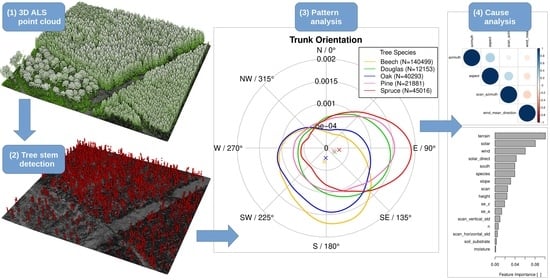
The study by Lamprecht et al. [1] has unintentionally revealed a preferred orientation of ALS detected spruce and beech trunks within a study site. This result raises the question whether ALS could be used to investigate the underlying cause of the orientation of tree trunks on larger scales. If so, tree trunk detection using ALS might be a powerful tool to address the species specific growth and inclination characteristics in response to site conditions, topography and wind.
1.2. Causes for Tree Inclination
Gravitropism describes the gravitative growth characteristics of plants. In particular, the trunk of a tree grows contrarily to the gravitative field, while the roots follow the gravitative field [2]. By asymmetric growth, trees are able to actively control their inclination. Lateral incidence of light, competition for light, continuous wind, or sudden disturbances like landslides, snow break or storms can cause a tree to deviate from gravitropism.
Phototropism causes plants to reorient their growth towards or against a light source [3,4]. Since trees try to maximize light absorption, a lateral incidence of light—as given in the mid-latitudes—is expected to result in trees inclined towards the equator. This effect has been verified for 256 Cook pines located around the globe by Reference [5].
Matsuzaki et al. [6] show that the stem inclination of trees can be actively influenced by the position of a fixed light source. In their experiment 90% of 212 investigated trees were inclined in down-slope direction, while a significant species dependent correlation between phototropism and gravitropism could be observed. The cause of this effect seems to be related to phototropism triggered by an uneven light supply in sloped terrains. In up-slope direction, the hill and the surrounding trees standing higher up the slope tend to cover the incidence of light, while in down-slope direction the lower standing trees facilitate light penetration. Ishii and Higashi [7] postulate that also understory trees adapt their trunk inclination for best possible utilization of the available light. Using a numeric model, they find a significant correlation between slope and trunk inclination for understory trees, but no effect for canopy trees at two test sites of evergreen trees with an area of and respectively.
In addition to phototropism, also soil movements and landslides can cause trees to incline with the slope gradient. The soil movements typically result in trees inclined downhill or uphill. Typically the trees try to recover gravitropism by asymmetric growth, resulting in bent stems with eccentric radii [8].
Wind is one of the major sources of mechanical loading on plants [9]. The complex interaction between the forest structure and the terrain results in small scale turbulences preventing a realistic prediction of the wind drag of a specific tree [9,10]. But, in general, a tree does not topple or uproot if the elastic restoring forces of the stem and roots can resist the combined wind and gravitational forces [9]. In consequence, trees grow adaptively and realign their structure to minimize wind drag, but maximize light capture. A continuous wind drag can make a tree realign its foliage permanently, resulting in windswept trees with foliage allocation in the prevailing leeward direction. Windswept crowns reduce the wind drag significantly and reduce the risk of stem or root damage [9,11]. Telewski [12] argue that the windswept growth is more likely the product of biomechanical properties than of a physiological thigmotropic growth response.
Nicoll and Ray [13] observe an adaptive growth of the root system of Sitka spruce in response to wind or site conditions. The roots of 100 randomly selected trees were characterized by an increase of structural root mass on the leeward compared to the windward side. Nicoll and Ray [13] conclude that the resulting asymmetric rooting structure reduces the tree’s vulnerability to windthrow. There are also indicators that a large proportion of branches in the total tree mass increases the windthrow risk of trees significantly [14]. In consequence, species with a low allocation of branch mass should be particularly resistant to wind.
Apart from the strength of the trunk, the root plate morphology, soil type and soil moisture define the resilience of a tree to external forces [15]. Also the rooting depth controls the anchoring of a root in the soil [16]. The numeric models of Fourcaud et al. [17] indicate that in clay-like soils, the rooting depth defines the root-soil plate and consequently the anchor strength. In sand-like soils, the shape of the rooting system determines the shape and size of the soil-root plate [17]. The results also indicate that the mechanical stress introduced by wind is highest in the superficial roots and the leeward roots. The soil moisture is an important factor that controls the resistive forces of the roots [10]. Heavy rainfalls accompanying storm events can weaken the anchoring of rooting systems and make trees vulnerable to toppling [10,15].
1.3. Stem Detection Using ALS
In recent years several methods for extracting tree stems using ALS have been developed [1,18,19,20,21,22,23]. Due to differing objectives, differing ALS acquisition designs and differing investigated forest types and structures, the accuracy of the trunk detection methods is hard to compare. In comparison to classic ALS driven tree crown delineation (see Reference [24]), all methods are able to extract vertical linear structures with a high reliability, and the precision of the tree positions is high. In general, two types of detection methods can be distinguished, heuristic methods and methods taking advantage of machine-learning techniques. With the downside of requiring training data, methods based on machine learning are expected to be transferable on stands and ALS data with various characteristics. Heuristic methods can be applied without training data, but are typically hard to parameterize and are typically not robust to differing forest characteristics.
The method of Lu et al. [18] takes advantage of the ALS intensity values to isolate points associated with trunks from leaf-off deciduous trees. The extracted points are used for a three-dimensional bottom-up trunk-growing process, while the assignment is controlled by a three dimensional and a planar distance threshold. To avoid false positives, the trunk length and the maximum height of the lowest trunk point are controlled by threshold values. Furthermore the identified trunks are used for crown delineation of 20 plots with a total area of and an average point density of 10 points/m2. The method achieves a detection rate of 84% and a precision of 97%.
Lamprecht et al. [1] identify tree trunks by creating ALS point cloud segments using a Divide & Conquer approach. Points associated with tree trunks are isolated from the canopy by estimating the crown base height and 3D-clustering. A principal axis is fitted to each cluster using a deterministic modification of the LO-RANSAC approach. The algorithm provides a vector model for each trunk detection, with attributes like root position, inclination angle and the compass direction. A validation with 109 TLS-measured trees in a plot of and an average ALS point density of points/m2 has shown a detection rate of 84% and a precision of 95%, while an RMSE of the trunk roots of could be observed.
The bottom-up approach of Shendryk et al. [20] uses full-waveform ALS data to delineate individual trees using tree trunks as seeding points. In extension to Lu et al. [18], next to an intensity filter, the ALS pulse width is used to filter points associated with trunks in range of 1 and 10 above ground. Finally, a three-dimensional Euclidean clustering is applied to identify individual trunks. Using 38 reference plots within a forest of a complex structure with a total area of , the algorithm has been applied to ALS data sets of two different point densities. By doubling the point density from 12 points/m2 to 24 points/m2, the tree detection rate increased from 56% to 67%, while the precision diminished from 62% to 61%.
Polewski et al. [19] propose free shape context descriptors to detect dead tree trunks in ALS point clouds. After a segmentation of the point cloud, a principal axis is fitted to each cluster using the M-estimator Sample Consensus method. For each axis, 3D free shape context descriptors are derived. After training and optimizing the shape descriptors with a genetic approach on an ALS tile of km2 with a point density of 30 to 40 points/m2, the algorithm is able to distinguish dead tree trunks from lining trees. The algorithm achieves an accuracy of 84.2% for 208 dead trunks and 340 living trees. The correctness of the principal axis is not discussed by the authors.
Amiri et al. [21] enhance the method of Polewski et al. [19] for identifying individual tree stems using high density ALS point clouds. With a Random Forest Classifier, points associated with tree stems are classified using 3D shape descriptors, covariance features and the normalized height. Initial linear segments are created based on points associated with the stems. These are merged to individual stems by hierarchical clustering. To describe a stem, a line is fitted by orthogonal distance regression and energy minimization. For two plots of and and an average point density of 300 points/m2, the method achieved a classification accuracy of up to 86% for 196 reference stems.
Most recently, Windrim and Bryson [22] publish new approaches to automatically detect trees and reconstruct stems using supervised deep machine learning methods using high resolution ALS point clouds. After detecting individual trees, points associated with the tree stems are extracted based on machine learning using voxel convolutions or neural networks. Finally segmented models of the main stems are fitted to gain information on the tree height, diameter, taper and sweep. The analysis has been conducted on 25 plots with an ALS point density of 300 points/m2 up to 700 points/m2 and 447 reference trees. The proposed methods achieve an overall tree detection accuracy of 77% up to 96% and an IoU (Intersection over Union) for stem detection of up to 52%.
As Chen et al. [23] have shown, trunk detections can be used to improve individual tree segmentation. Similarly to Lamprecht et al. [1] points associated with the tree trunks are identified by estimating the crown base height. Trunks are derived by a two-dimensional mean shift clustering using a flat kernel function with a bandwidth associated with the trunk diameter. Using the identified trunks as initial points, the mean shift individual tree segmentation could be improved significantly. The analysis has been conducted for 20 reference plots with a total area of , an average ALS point density of 15 points/m2 and 1779 reference trees.
Although the SkelTre method, developed by Bucksch et al. [25], is able to derive a point skeleton from any point cloud, it has been designed to derive the three dimensional structure of trees—inherently providing information on the stem orientation—based on high density laser scans. The algorithm creates an initial graph based on an octree [26], while a robustness criterion ensures an appropriate linkage of the graph’s edges even for noisy input point clouds. By labelling each edge with its direction, the octree-graph is locally reduced to achieve a Reeb-graph [27]. Finally, the graph is embedded to the original point cloud to provide localized information on the skeleton.
1.4. Related Work
A systematic analysis of the ALS-derived trunk inclination and orientation angles is given by Razak et al. [28], which investigates the effect of landslides using high density ALS in an alpine region. As base data, they use a point cloud with an average point density of 170 points/m2 and an approximate area of about km2. They delineate the tree crowns using the TreeVaW [29] algorithm, which achieves an overall accuracy of 84.8% using 560 terrestrially measured reference trees. The tree inclination and tree orientation have been derived with the SkelTre method [25] which tends to over-predict both variables. A regression model of the form achieves an of . With a model of the form —which violates the cyclic character of the compass angles—they observe values of up to at a reference height of m. They find that trees located in landslide zones are more inclined and dispersed at different orientations compared to the control group.
2. Objectives
The studies presented in Section 1.3 focus on the detection of tree stems within study areas smaller than 2 km2 only. To the knowledge of the authors no evaluation of the trunk inclination and orientation properties—in particular on larger scales—has been carried out so far. In the given study the following hypotheses are evaluated empirically to verify whether the ALS detected tree trunks show systematic inclination patterns, and whether these patterns match the known causes for tree inclination:
Hypothesis 1.
Preferred stem orientations can be found using ALS derived trunk vectors.
Hypothesis 2.
Trunks preferentially lean down-slope.
Hypothesis 3.
The tree inclination and orientation depend on tree species.
Hypothesis 4.
Trunks preferentially lean leeward.
Hypothesis 5.
The scan direction does not affect the observed trunk inclination and orientation.
Hypothesis 6.
Soil properties, like soil type and moisture, affect the trunk inclination.
3. Materials and Methods
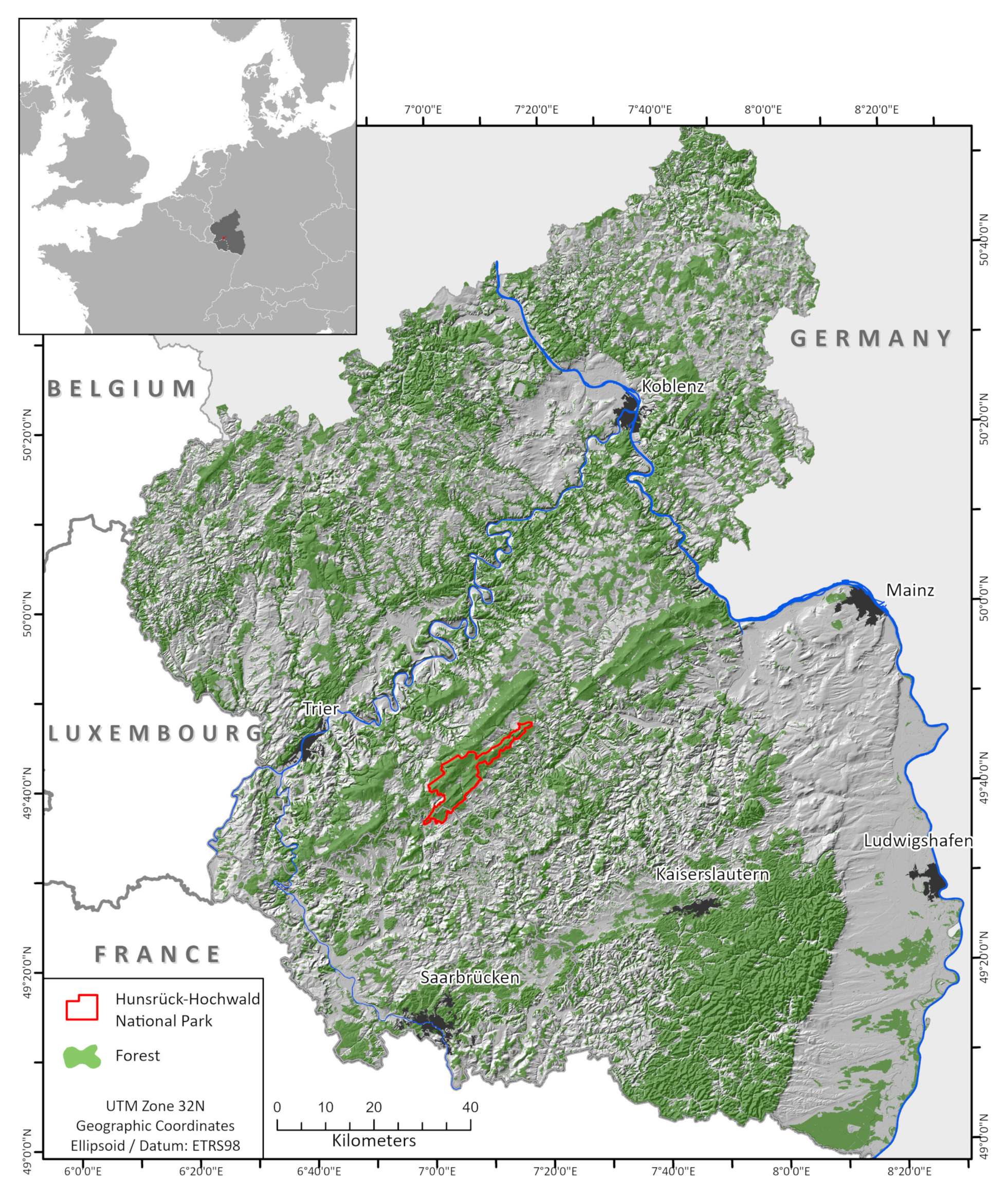
3.1. Study Area
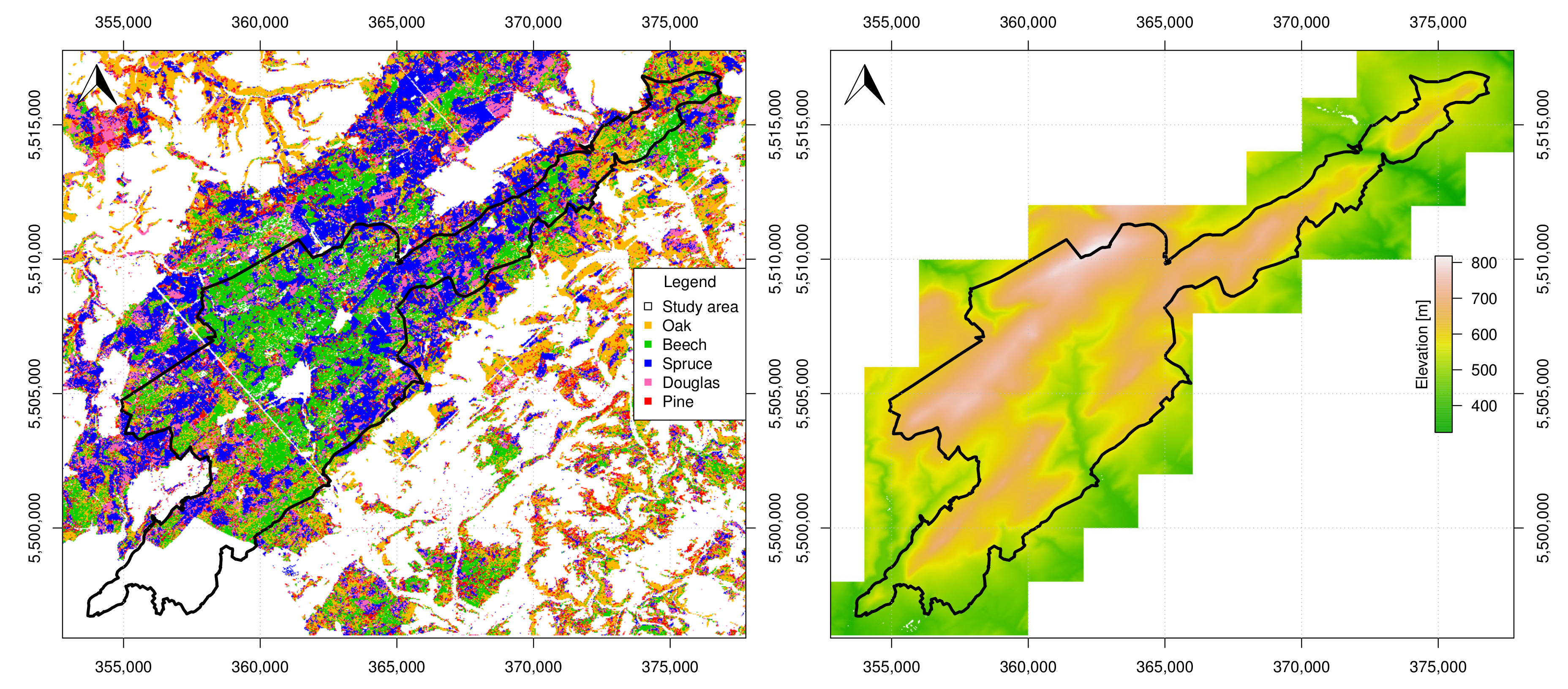
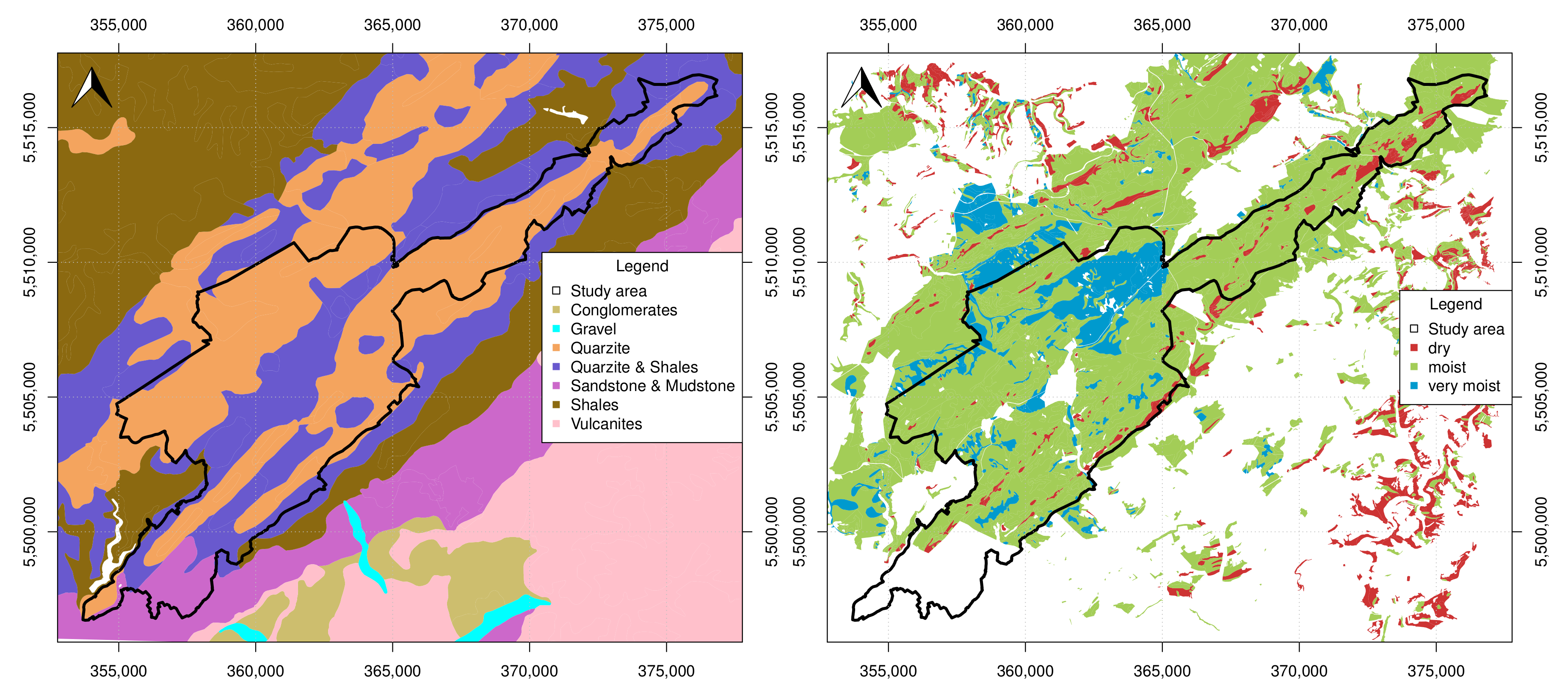
The study area of Hunsrück-Hochwald National Park with an area of km2 is located in Rhineland-Palatinate and Saarland, Germany (Figure 1). From its southwestern extent it follows a low mountain range for about 30 to its northeastern extent (see Figure 2). Its moderate climate of the mid-latitudes results in good conditions for sustainable forestry. The area is dominated by 44.9% European beech (Fagus silvatica) and 33.2% Norway spruce (Picea abies), 10.0% Sessile oak (Quercus petraea), 8.2% pine (Pinus sylvestris) and 3.6% Douglas fir (Pseudotsuga menziesii). Less common are European larch (Larix decidua), European white birch (Betula pendula) and other species. The soil substrate is dominated by quarzites and shales of the Devonian, and sandstone and mudstone of the Permian [30].
3.2. Data
3.2.1. ALS Data
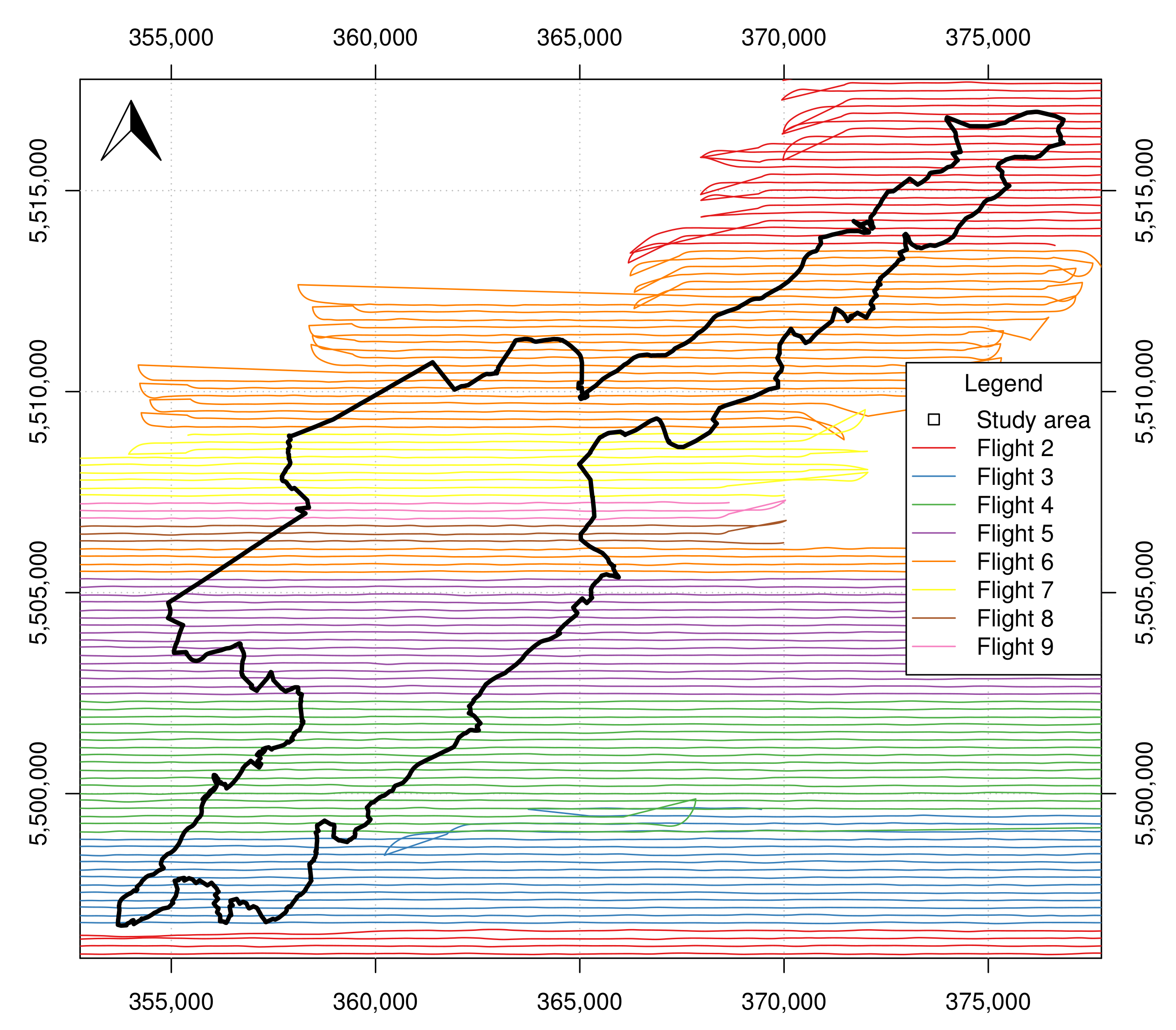
The ALS data used in this study has been acquired during nine flights from 24 March to 7 April 2015 using a Riegl Q560 [32] under leaf off conditions. The flights have been strictly conducted in east-west, or west-east direction with an average swath width of about 200 (Figure 3). The mean altitude has been about 600 resulting in a footprint diameter of about and an average pulse density of pulses/. The 220 ALS tiles have been provided by the state surveying and geoinformation service of Rhineland-Palatinate (LVermGeo) in the form of pre-classified (ground, vegetation and other classes) .las-files with an extent of 1 × 1 each. Each ALS point is labeled with its GPS timestamp expressed as second of week. For each flight the GPS tracks have been provided in .csv format.
3.2.2. Terrain and Canopy Models
Both a terrain and a canopy model are derived for each ALS tile by filtering points representing the surface in a first step and applying a Delaunay triangulation in a second step. The triangulation allows for a linear interpolation of the elevation within the given tile. In detail, to identify points representing the terrain, the points classified as ground are thinned with a duplicate point filter identifying local minima with a radius of (see filters.surface of Lamprecht [33]). Similarly, to identify points representing the canopy, the points classified as vegetation are thinned with the same duplicate point filter extracting local maxima with a radius of .
3.2.3. Scan Direction
Since the ALS points do not contain information on the scan direction, it is calculated using the supplementary GPS files. For each point of interest, the two GPS coordinates with minimum time difference are selected. Based on the time difference, the acquisition coordinate is interpolated as the linearly weighted average of both GPS coordinates. With this interpolated GPS coordinate, the line of sight (scan vector) linking the position of the laser scanner and the point of interest is derived.
3.2.4. Tree Species
To receive information on the tree species, the high resolution forest information layers of Stoffels et al. [31] are used. This data set provides information on the five most common tree species—European beech, Douglas fir, Sessile and Pedunculate oak, Scots pine and Norway spruce—in a spatial resolution of 5 × 5 m2. Except for the most southwestern area, the classification layer covers the study area completely, while an overall classification accuracy of about 76% is achieved.
3.2.5. Wind
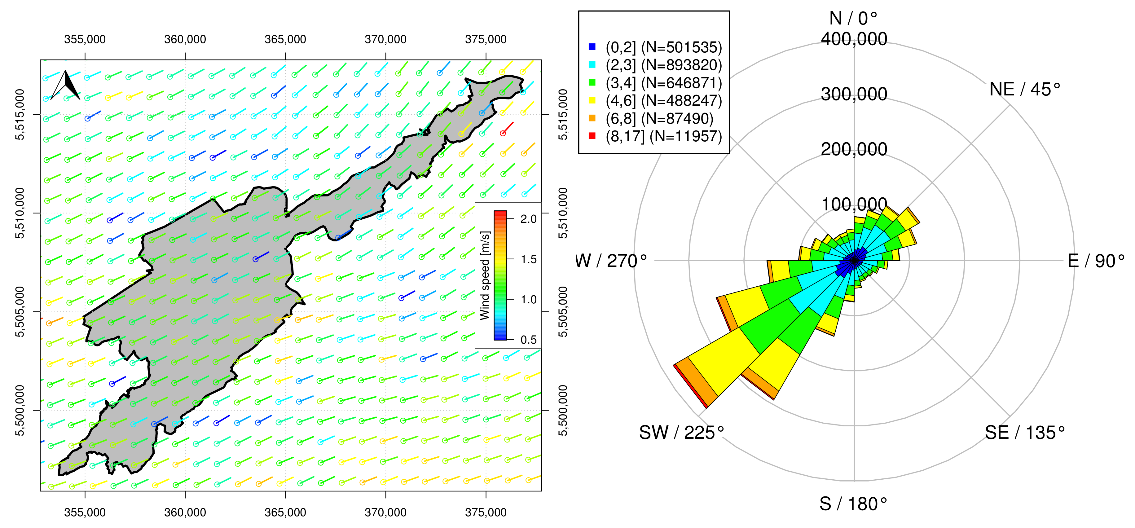
Complex forests with dynamically restructuring trees in combination with hilly terrains make a deterministic prediction of the time and spatial scale dependent wind flow, eddies and turbulences practically impossible [9]. Thus, in this study, only the effect of the prevailing wind direction is considered. The daily wind direction and wind speed datasets of the TRY project [34] are used as base data. These provide information at a reference height of 10 above ground and a spatial resolution of 10 × 10 . To represent the prevailing wind direction and wind speed, in this study the wind vectors are averaged over a 15 year period from January 1998 to December 2012. As Figure 4 illustrates, in the study area the wind is typically directed from West-South-West at average wind speeds below /. In the Northwest of the study site, the wind turns to the Southwest.
3.2.6. Soil Properties
To inspect the influence of the soil, the official soil region map of Germany [35] is used. Since the given soil classification does not allow for a spatially explicit distinction between different soil types, the dominating soil substrates are extracted as illustrated in Figure 5 (left). In addition to the soil type, an ecological site classification [30]—provided by the state forest service of Rhineland-Palatinate (Landesforsten RLP)—is used to investigate the effect of soil moisture on the trunk inclination. One product of the ecological site classification is a soil moisture classification with 12 soil moisture regimes. In general, the study area is well supplied with water. The given regimes are re-sampled to three classes dry, moist and very moist as illustrated in Figure 5 (right).
3.3. Methods
3.3.1. Stem Detection
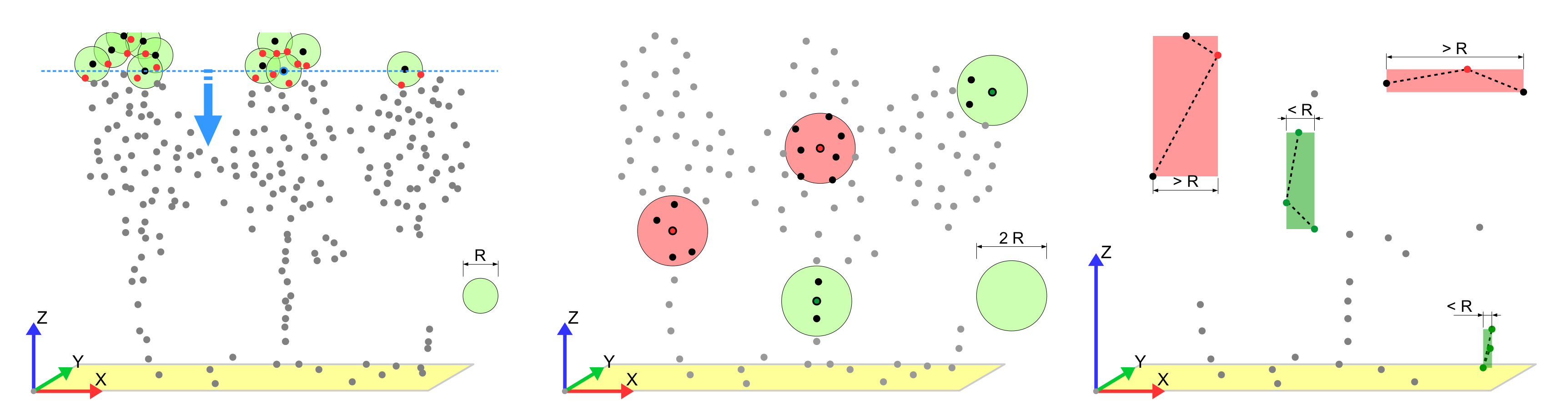
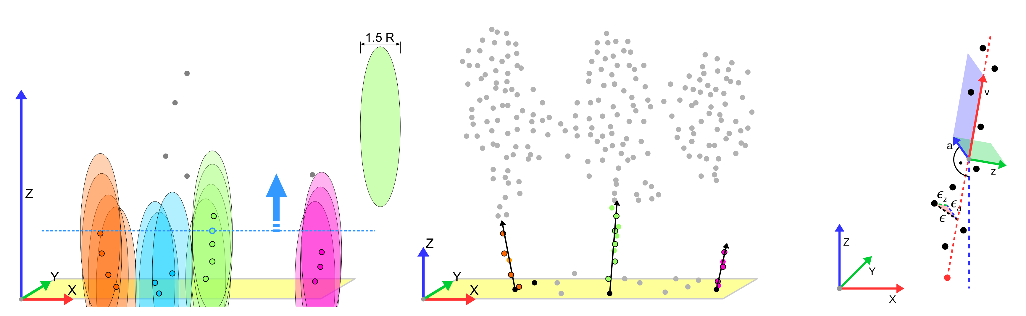
For the given study, a stem detection algorithm has been developed, which shall identify vertical linear structures most probably representing stems. To limit the computational effort and be independent from training data, heuristics are used to identify points associated with the stems. The algorithm is organized in three steps: point filtering (identifying points below canopy form vertical lines), clustering (identifying individual trunks) and vector fitting (fitting a regression vector to each trunk). A fundamental parameter of the algorithm is the radius R. Since this parameter should be in the scale of the minimum expected trunk distance, R is set to by expert decision.
3.3.1.1. Point Filtering
The trunk detection algorithm developed for the given study assumes that ALS points arranged in isolated vertical lines close to the ground represent tree trunks. To facilitate the isolation of linear structures, in a first step a duplicate point filter is applied to all points classified as vegetation (Figure 6, left). In detail, the filter sweeps from top to bottom, while for each point currently observed, all points within radius R are removed. In a second step, only points with less than two neighbors within radius 2R remain (Figure 6, center). In particular volumetric structures—like tree crowns—are removed by this filter, because the previously applied duplicate point filter ensures point distances of at least R. The previous filters tend to retain isolated points at the fringe of tree crowns. Thus, a vertical orientation of neighbored points needs to be ensured. For each point, the closest two neighboring points are investigated, while the z-axis is scaled by factor 2 to prefer a vertical assignment. If the horizontal extent of the three points is less than R, all three points remain (Figure 6, right).
3.3.1.2. Clustering
To identify isolated lines in the previously filtered point clouds, the points are clustered. The clustering algorithm sweeps from bottom to top (Figure 7, left). A point is assigned to the most frequent cluster of its neighboring points within radius 1.5R. If no neighboring point has already been assigned to a cluster, the point defines a new cluster. To take into account the vertical structure of the trunks, the z-axis is scaled by factor before applying the clustering. To remove remaining linear structures in the top of the trees with no connection to the ground, only clusters with a gap to the ground smaller 0.6 are retained, while h represents the height above ground for each point of the cluster. To use the full number of available trunk points, all original ALS points with distance less than R to any of the cluster points define the final cluster.
3.3.1.3. Vector Fitting
A regression vector is fitted to each previously identified trunk cluster. Since the clustering algorithm tends to retain dispersed points at the bottom of the tree crowns, these points might distort the vector orientation. Thus, a consensus set is created by applying the MSAC [36] approach with threshold R to all point pair combinations of a cluster. The first Eigenvector of the consensus set represents the desired regression vector (Figure 7, center). Consensus sets with less than 4 points are omitted.
Based on the regression vector, a local coordinate system with the axes v, z and a is defined (Figure 7, right). The origin of the coordinate system corresponds to the average coordinate of the trunk points, while the Eigenvector defines the v-axis. The a-axis is oriented perpendicular to the regression vector and the global z-axis. Finally, the z-axis is oriented perpendicular to the global x- and z-axis.
The trunk root is defined as the intersection point between the regression vector and the terrain model. Each trunk vector provides its inclination or zenith angle , referring to the angular deviation of the stem from the vertical orientation ( 0). The orientation or azimuth refers to the compass direction of the stem, defined as the clockwise planar deviation from the North ( 0).
3.3.1.4. Vector Uncertainty
Using its local coordinate system, the residuals of a trunk vector fitted to n points are split up in a vertical and a horizontal component (see Figure 7, right). Similar to a two dimensional regression line, the standard error of the inclination is calculated with Equation (1). Accordingly, the standard error gives information on the uncertainty of the trunk azimuth.
Similar to the two dimensional regression, the inclination is assumed to follow the Student’s t-distribution with degrees of freedom. The p-value is calculated according to Equation (2). The function corresponds to the cumulative distribution function of the Student’s t-distribution with test value x and degrees of freedom.
3.3.2. Trunk Features
To evaluate the hypotheses, each detected trunk is labeled with its inherent vector features and the attributes of the data layers. To increase readability, a set of an arbitrary higher order property is derived by a function and according to Equation (3). Each trunk t is characterized by the inclination angle and the compass orientation of its three-dimensional regression vector. Its root is defined by the intersection point between its vector and the DEM. The attributes and give information on the uncertainty of the vector in inclination direction and compass direction respectively (see Section 3.3.1.4). Using the p-value of the trunk inclination is derived (see Equation (2)).
Features related to the ALS properties are aggregated from the points used to fit the trunk vectors. In particular, the scan vectors are averaged and split up into a vertical scan angle and a horizontal scan direction . In addition, the horizontal () and vertical () standard deviations of the scan vector are calculated.
The tree species, soil moisture and soil substrate classes are assigned by intersecting the trunk root coordinates with their raster cell or polygon. The wind direction and wind speed for each trunk is determined by a Cressman interpolation [37] of the wind vector rasters with a radius of 1 .
The site , and are derived for each trunk by inspecting the seven terrain points closest to the trunk root. Due to the planar character of the ground points, their third Eigenvector provides the aspect and slope, while the elevation is extracted from their average z-coordinate.
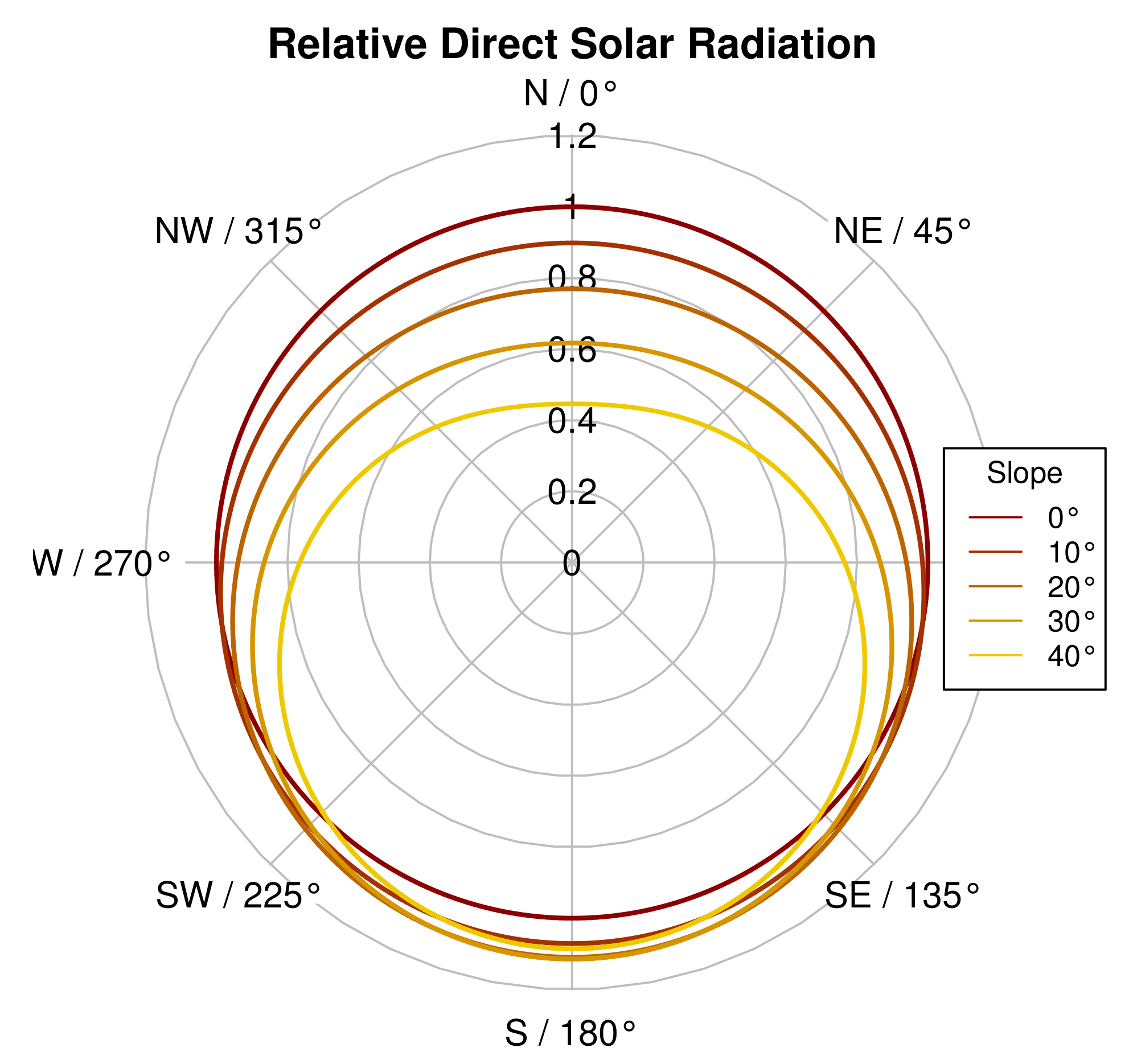
As a measure of phototropism, the relative direct solar radiation is calculated for each tree according to Gassel [38] using Equation (A1) (see Appendix A). The radiation is calculated for each tree based on its geographic latitude, site aspect and slope assuming solar noon at mid of summer. The effect of the site aspect and slope on the relative direct solar radiation is illustrated in Figure 8.
3.3.3. Regression Models
To analyze underlying causes for stem inclination, for each trunk t its inclination is predicted using weighted least squares regression. Weighted regression is used to suppress biases caused by very frequent trunk inclinations and orientations. Only attributes potentially causally related to the inclination are considered to derive the predicted inclination . Next to the variables of interest (slope, tree height, tree species, wind speed, soil moisture, soil substrate and scan angle), attributes associated with the uncertainty of the trunk vectors (, and ) are considered since they might relate to random effects.
To make qualitative statements on potential underlying causes for specific inclination directions, the trunk orientation is assumed to be a linear combination of two dimensional explanatory vectors. To implement this concept, each directed variable defines an explanatory vector as illustrated in Equation (4), while for each trunk its orientation is modeled by creating pairwise coupled equations according to Equation (5). By multiplying scalar variables with these vectors, interaction terms can also be considered. Solving the given equation system using weighted least squares regression provides the desired regression coefficients which are used to calculate the predicted trunk orientation .
Please note that the signs of the regression coefficients give information on the direction of the underlying effects. The coefficient —corresponding to a directed intercept—shall allow for a systematic inclination to the South.
To avoid biases caused by the uneven frequency of the observed stem orientations, the equations of the regression models are weighted by the p-value of the trunk inclination times the inverse circular density of the trunk orientation. The density of the trunk orientation is determined by a kernel density estimation using the bandwidth selection procedure of Sheather and Jones [39].
3.3.4. Feature Selection
To pre-select relevant features, the trunk inclination as well as the orientation are modeled with Random Forest regressors of 500 trees and 50,000 randomly selected trunks. The default parametrization of the ranger package for R [40] is used. Missing numeric values are filled by mean imputation, while categorical values are imputed by random sampling of the non-missing values. Attributes with low feature importance are neglected for further analyses. After identifying the most relevant features, several knowledge driven linear models are fitted, while equations with missing values are omitted (see Section 4.5). This iterative procedure shall guarantee the selection of robust knowledge driven models to reveal potential underlying causes for the trunk inclination.
Due to the circular character of the orientation, the model residuals tend to be bimodally distributed. Also the inclination model tends to violate the homoscedasticity assumption. To still be able to make qualitative statements on the effects, the confidence intervals of the regression coefficients are empirically determined by bootstrapping. Each regression model is fitted 10,000 times to differing random samples of 1% of the training dataset. Finally the inclination and orientation models are fitted to the full training dataset. Model coefficients not significantly differing from zero (99% significance level, respectively 98% confidence interval) are discarded, or interaction terms are added. Factorial variables are omitted, if the coefficients of at least two categories do not differ significantly (99% significance level, respectively 80% confidence interval of each coefficient).
3.3.5. Training and Validation
The trunk detection algorithm of Section 3.3.1 is applied to all ALS tiles of the study area. Since border effects might affect the detection of trees at the edges of the tiles, all trunks with distance below 5 to the tile extends are disregarded for further analyses. Trunk vectors with a high vector uncertainty can lead to an inaccurate inclination and orientation. If the inclination error exceeds the inclination angle, the trunk orientation can even topple. These effects have the potential to cover systematic orientation patterns, since they appear as noise. For this reason only significantly inclined trunks— significantly different from zero—are further investigated. The remaining trunk detections form the set T. Of the data set, 70% is used for training and 30% for validation .
The accuracy of the trunk inclination prediction is assessed with the ordinary coefficient of determination . To adress the accuracy of the modelled orientation —in addition to the ordinary provided by the regression model—the angular residuals (see Equation (6)) are examined. The mean direction [41], as well as the circular standard deviation [41] describe the location and dispersion of the circular data. Based on the orientation vector (cf. Equation (5)), the average variance explained by each directed explanatory variable is calculated to assess its explanatory power. The explained variance of a directed explanatory variable with regression coefficient corresponds to the scalar product .
4. Results
4.1. Stem Detection
In total 1,147,633 stems have been detected, while 846,851 stems have been located within the study area. The partial coverage of the ground data results in missing data within the borders of the study area for soil moisture (10.6%) and tree species (11.5%). Since the given study shall provide a proof of concept only, only the plausibility is checked instead of an accuracy assessment of the stem detection. In particular, a strongly species-dependent detection rate might affect the results, since it would indicate problems of extracting the linear structures under certain stand characteristics.
Table 1 illustrates the percentage of area covered by each tree species (see Section 3.2.4) compared to the amount resulting from the stem detection. A chisquared goodness-of-fit test indicates that the detected species differ significantly from the species distribution provided by the classification layer. In particular, the amount of spruce and beech detections are higher than the area, while Douglas, oak and pine are under-represented by the stem detection. Since the surface area does not provide information on the actual stand density, no final conclusion on detection rates can be drawn. But, since the algorithm seems not to fail entirely for a specific species, the detected trunks seem to be suitable for further analyses.
4.2. Selection of Trunks
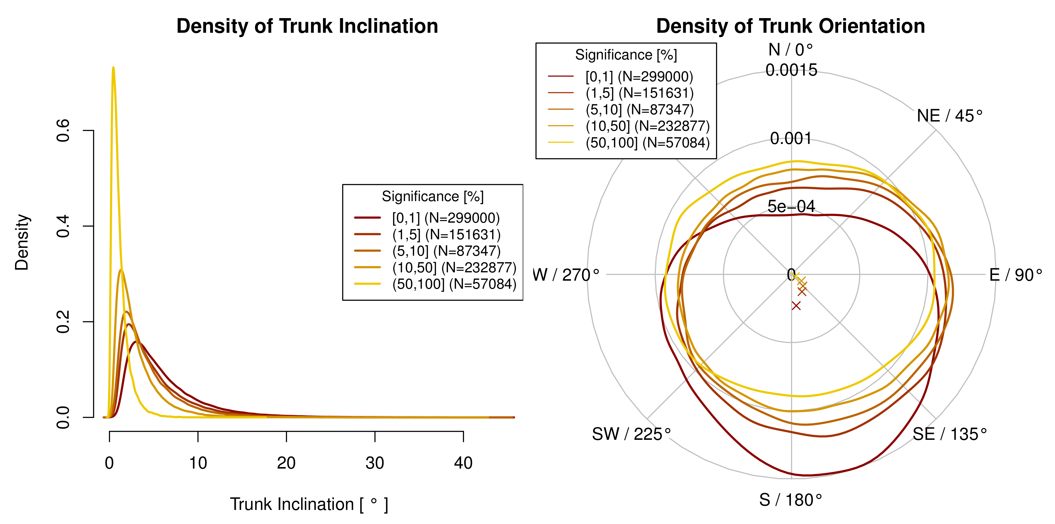
Figure 9 illustrates the effect of the p-value on the trunk inclination and orientation. By selecting significantly inclined trees only, the probability of an erroneous trunk orientation—due to randomly inclined observations—is reduced. Per definition, with decreasing significance levels, preferably trunks with high inclination angles are selected (Figure 9, left). Also with decreasing significance levels, a preferred South orientation of the trunks is revealed (Figure 9, right). To gain clean data, the authors have decided to choose a significance level of 1% resulting in a data set T of 299.000 trunks.
4.3. Stand Characteristics
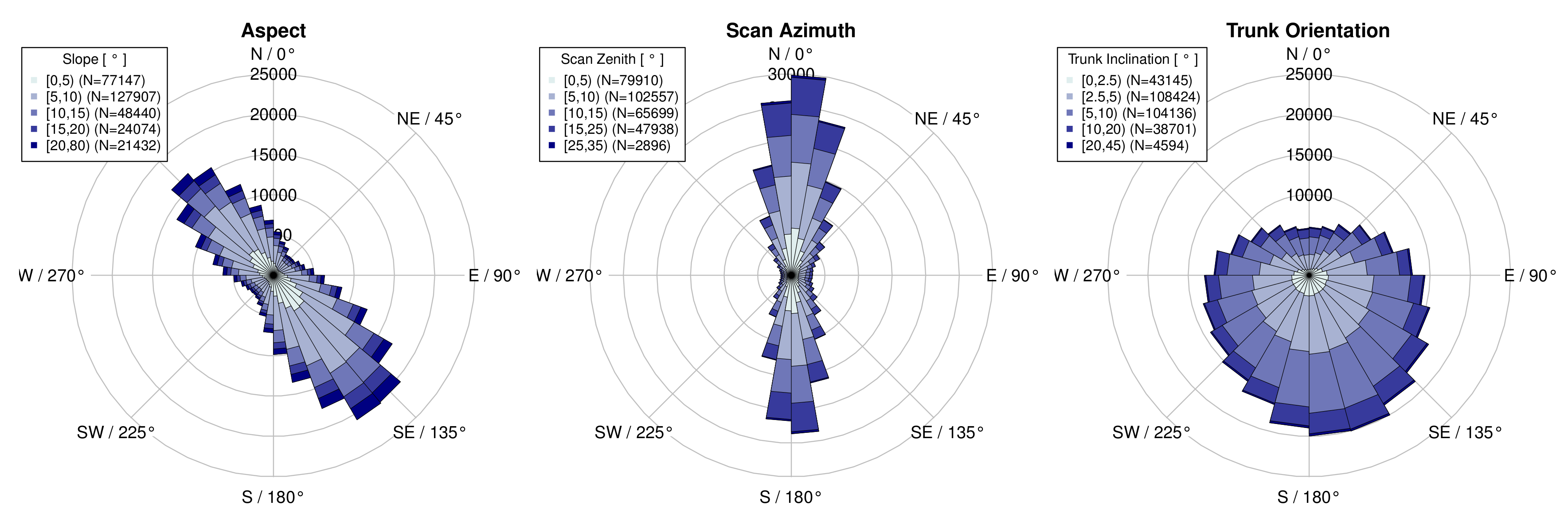
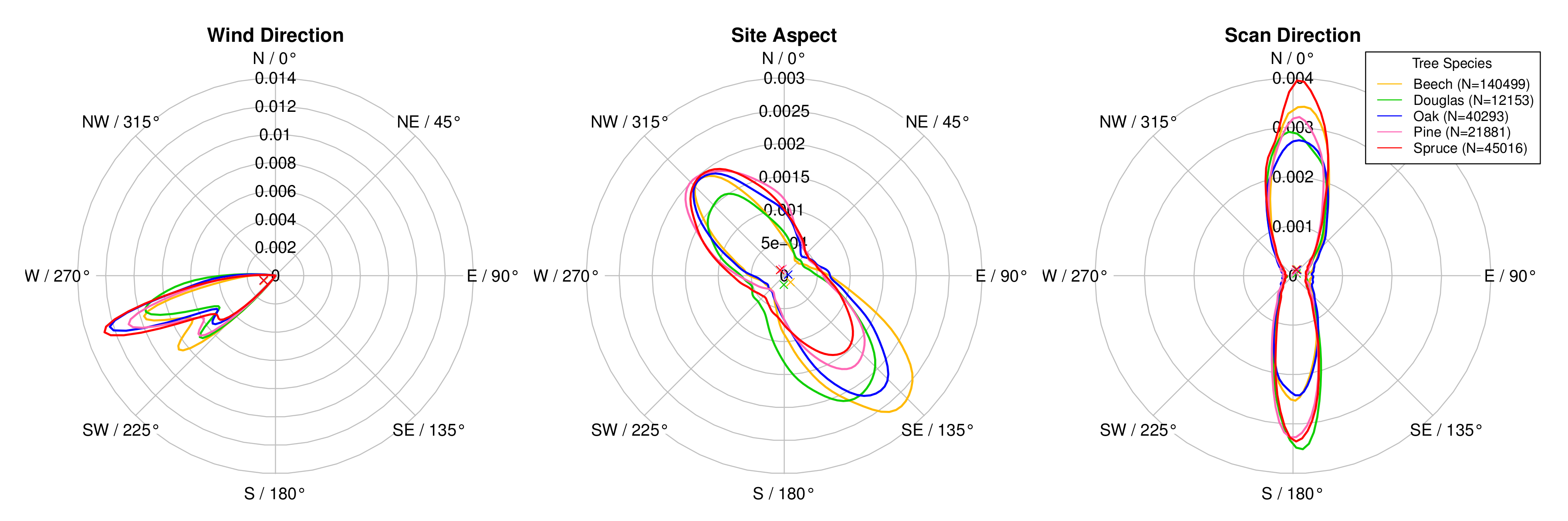
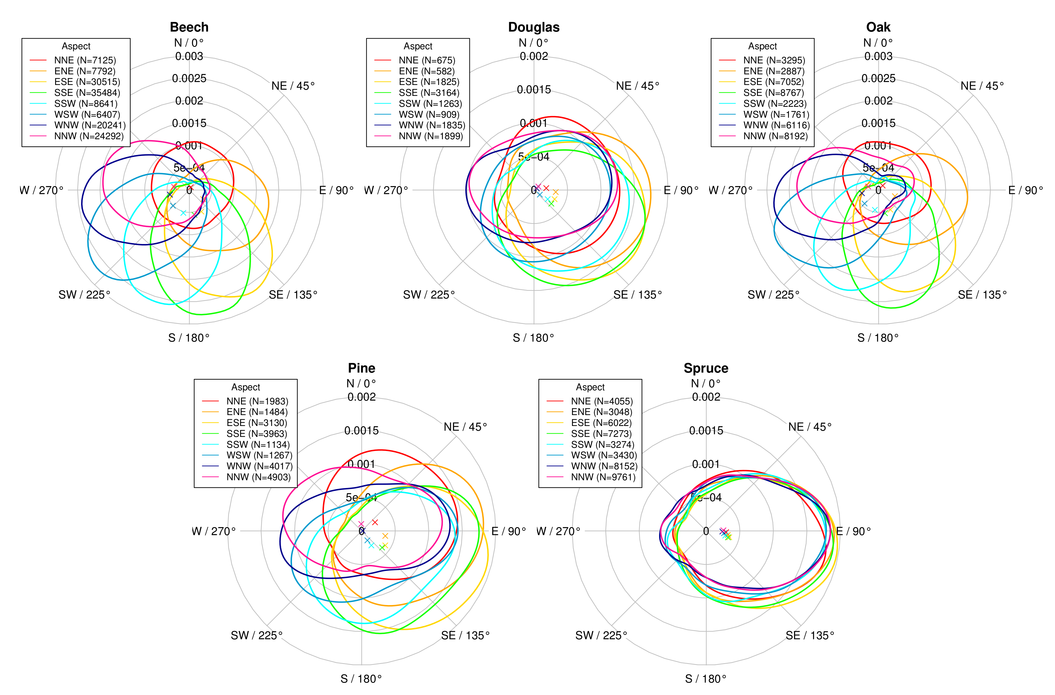
Figure 10 illustrates the site aspect, scan direction and observed trunk inclination for all significantly inclined trunks. Due to the orientation of the mountain range, most sites are oriented to South-East or North-West. With less than 3%, trees on slopes with an inclination greater than 25 are rare. The regular ALS flight pattern causes the trunks to mostly be scanned from the North or the South. 95% of the trunks are inclined less than 15. The trunks preferably lean to South-Southeast, with an average orientation of about and a circular standard deviation of . A Watson’s test for circular uniformity [42,43] confirms that the trunk orientation differs highly significantly from a uniform distribution, supporting Hypothesis 1.
Table 2 shows that regardless of tree species about 67% to 74% of the detected trunks are located on Quarzite sites and about 26% to 32% are located on mixed Quarzite & Shales sites. The portion of trunks located on pure Shales is minor. 82% to 86% of the trunks are located on moist sites. About 15% of the beech and spruce can be found on very moist sites, while about 10% of the Douglas and pine are located on very moist sites. With 10%, oak can preferably be found on dry sites rather than on very moist sites.
Figure 11 shall highlight potential species specific site characteristics, which might affect the modeling procedure. Although the local wind regime is characterized by topography and forest structure, the mean wind direction indicates an almost similar general wind exposition for all tree species. The spatial distribution of the trees lead to a species dependent site aspect. In general, the orientation of the mountain range results in most of the trees facing North-West, respectively South-East. Beech and Douglas tend to be located on sites facing South-East, while spruce and pine can mostly be found on sites facing North-West.
4.4. Preliminary Analysis
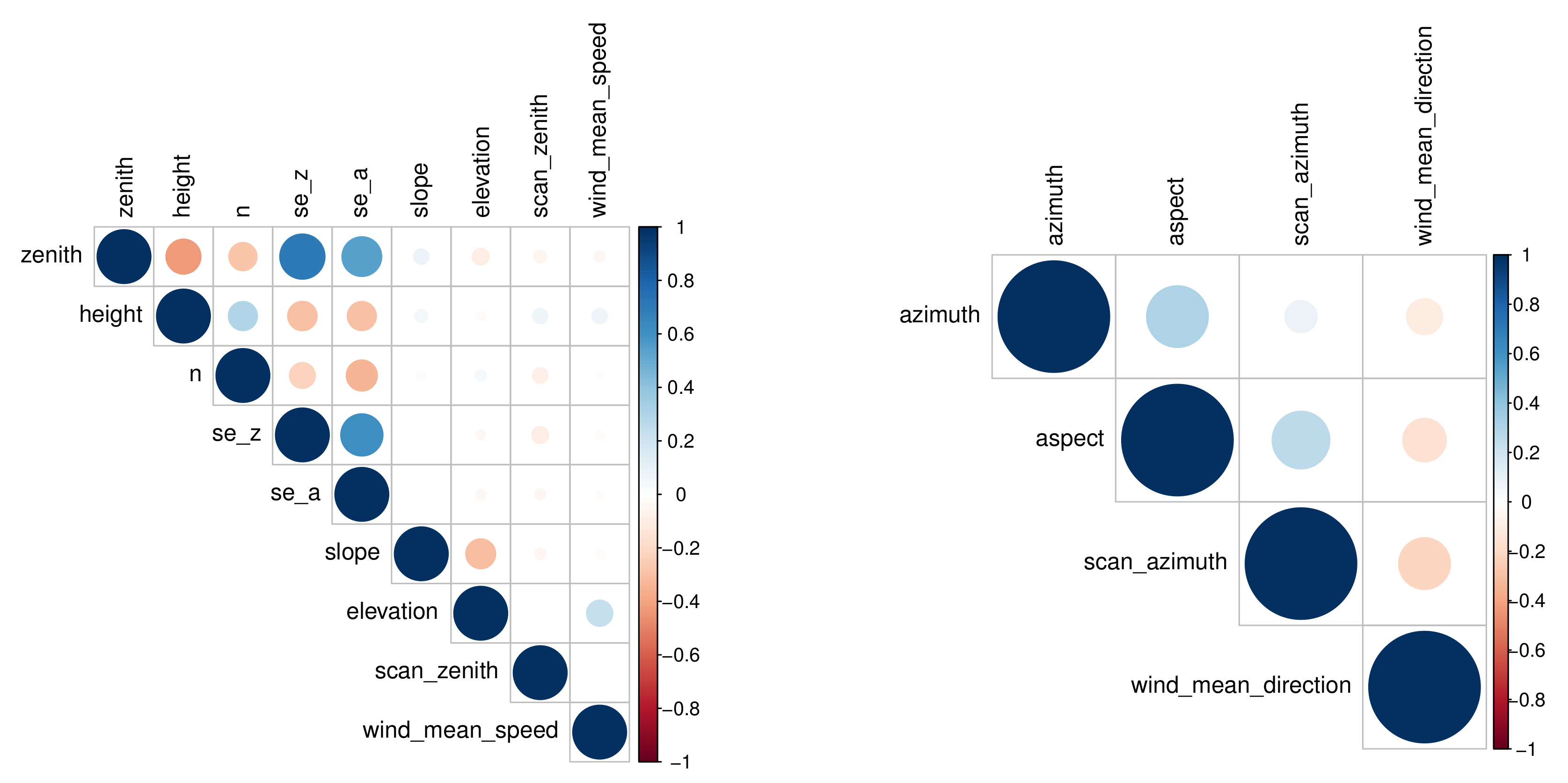
Figure 12 illustrates the Pearson’s product moment correlation coefficients of the trunk features. For the directed variables, the circular variant [42,43] is used. A strong correlation between the trunk inclination () and variables associated with the vector uncertainty is given. With increasing uncertainty—high , high , low n—high inclination angles can occur at random. The negative correlation of the tree height with the trunk inclination might be caused by the increased vector uncertainty. The trunk orientation is positively correlated with the site aspect. A slight negative correlation with the wind direction and a slight positive correlation with the scan direction can be found. But, these apparent correlations could be caused by coincidence due to the orientation of the mountain range and the stripe-wise ALS scanning pattern.
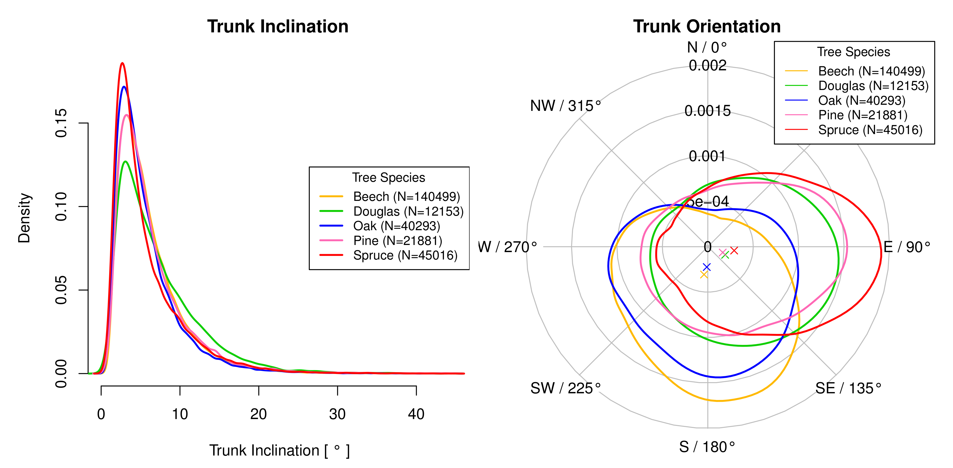
As Figure 13 and Table 3 illustrate, the observed trunk inclination and orientation depend on the tree species. A Kruskal-Wallis rank sum test indicates significant differences of the average inclination between the species. More interestingly, the trunk orientations between the species differ highly significantly. In particular, deciduous trees tend to lean to the South, while conifers tend to lean to the East. The first observation is an indicator for phototropism, the latter might be caused by wind.
These observations are in accordance with Table 4, which summarizes the amount of trunks inclined in the explanatory directions. About 70% of the deciduous trunks are inclined to the South, compared to 54% of the conifers. About 64% of the conifers lean leeward, compared to 41% of the deciduous trees (cf. Hypothesis 4).
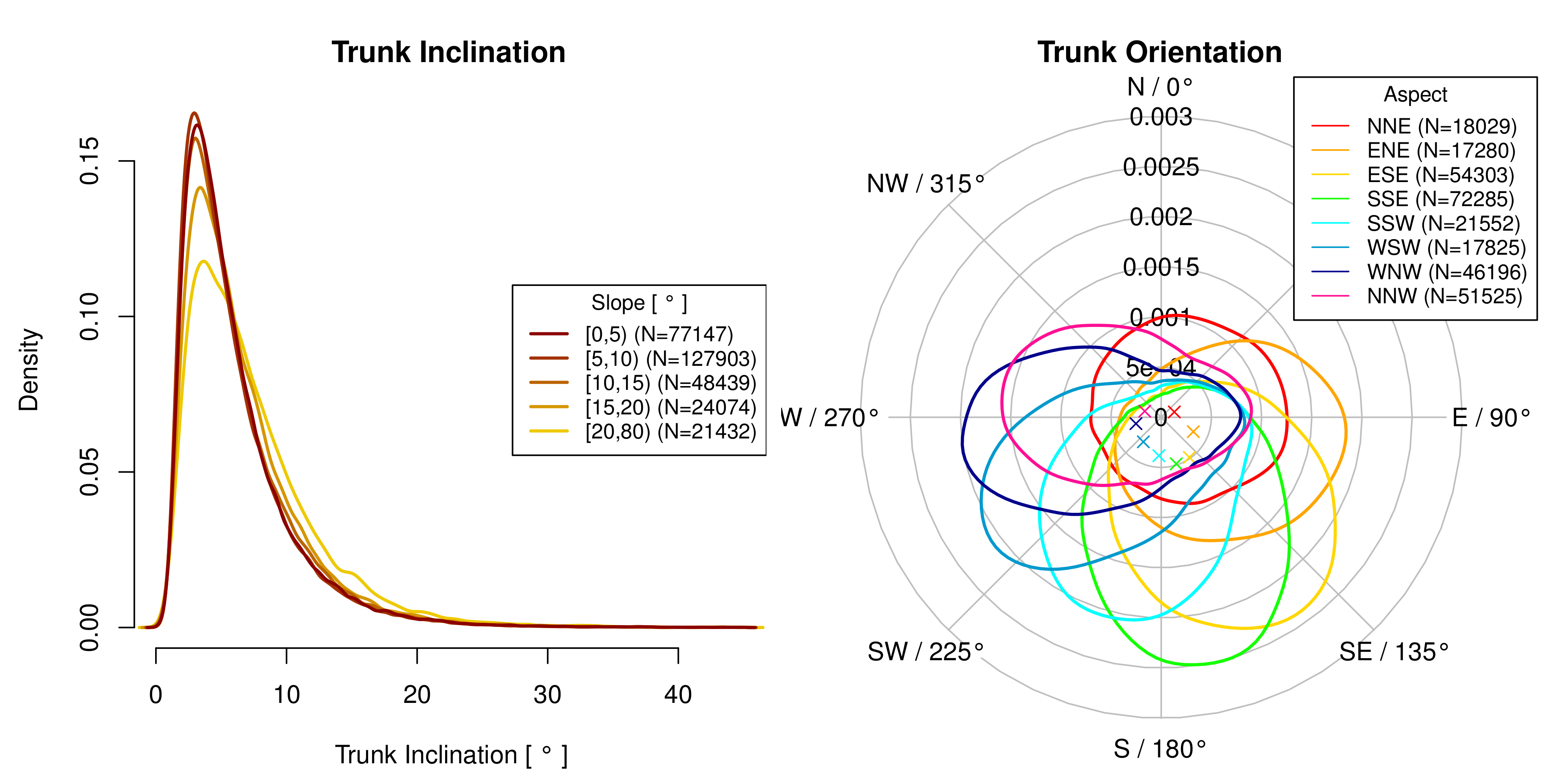
Supporting Hypothesis 2, Table 4, shows that 71% of the trees are inclined down-slope. The effect of the terrain is highlighted in Figure 14. In general, increasing inclinations of slopes result in increased inclination angles, while the orientation follows the site aspect systematically with a general trend to the South. This observation is in accordance with the interaction between the site aspect and phototropism, since a site facing to the sun facilitates light capture compared to a site facing to the North.
Figure 15 illustrates that this effect is highly species dependent. Beech and oak seem to be highly affected by the interaction between phototropism and the terrain, while the site aspect has almost no influence on the orientation of spruce.
Table 4 also indicates an effect of the scan direction on the observed trunk orientation (Hypothesis 5). But, the regular ALS flight pattern in combination with the uneven distribution of the tree species in the mountain range makes an autocorrelation with the scan direction highly probable. The same is true for a potential autocorrelation between the other explanatory variables. In consequence, for final conclusions the regression models are investigated.
4.5. Regression Models
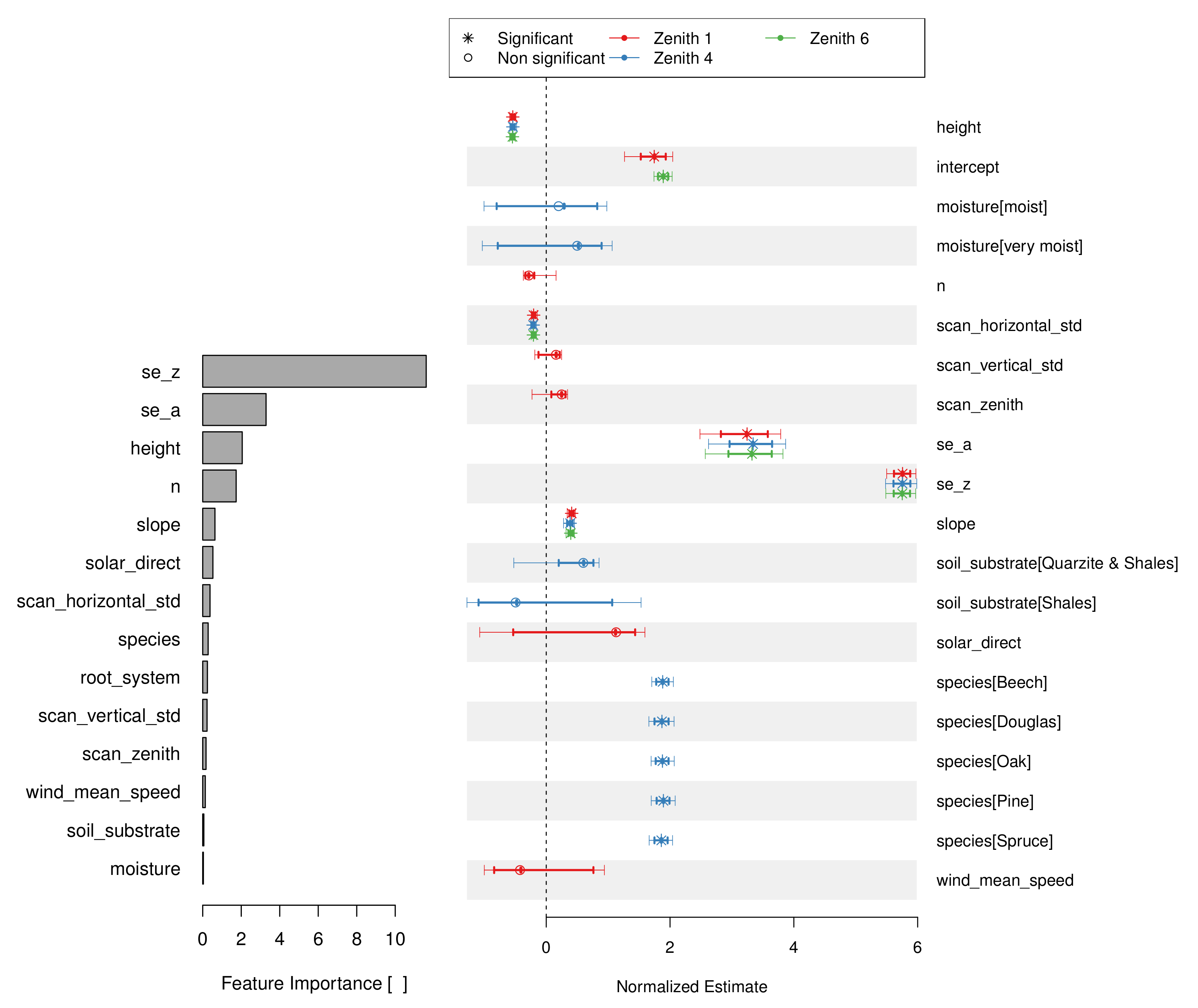
4.5.1. Trunk Inclination
Figure 16 illustrates the feature selection procedure with the feature importances of the Random Forest regressor and six linear regression models with differing features and interaction terms. Table 5 provides information on the partial and total of all six linear models. With an out of the bag of , the Random Forest regressor performs slightly better than the linear models, with values ranging from to .
The coefficients of the control variables and —both associated with the uncertainty of the trunk vectors—are significantly different from zero for all linear models, and dominate the models by their explanatory power. The variable is positively correlated with the trunk zenith angle, since with increasing uncertainty large zenith angles can occur at random. The tree height is negatively correlated to the trunk inclination, which might either be caused by the uncertainty of the vectors or by the need of tall trees to align vertically to avoid toppling.
Despite its low explanatory power with just about 2% of variance explained, the slope inclination is positively correlated with the trunk inclination. Supporting Hypothesis 2, this is a first indicator for a terrain dependent inclination of the trunks. In contrast to Hypothesis 5, a slight, but significant negative correlation between the scan direction and the inclination angle can be observed.
The models imply that none of the factors tree species, soil substrate or soil moisture affect the trunk inclination significantly. Based on the given data, the mean wind speed as well as the direct solar radiation seem not to influence the trunk inclination significantly. In addition, the control variables n and seem not to affect the trunk inclination.
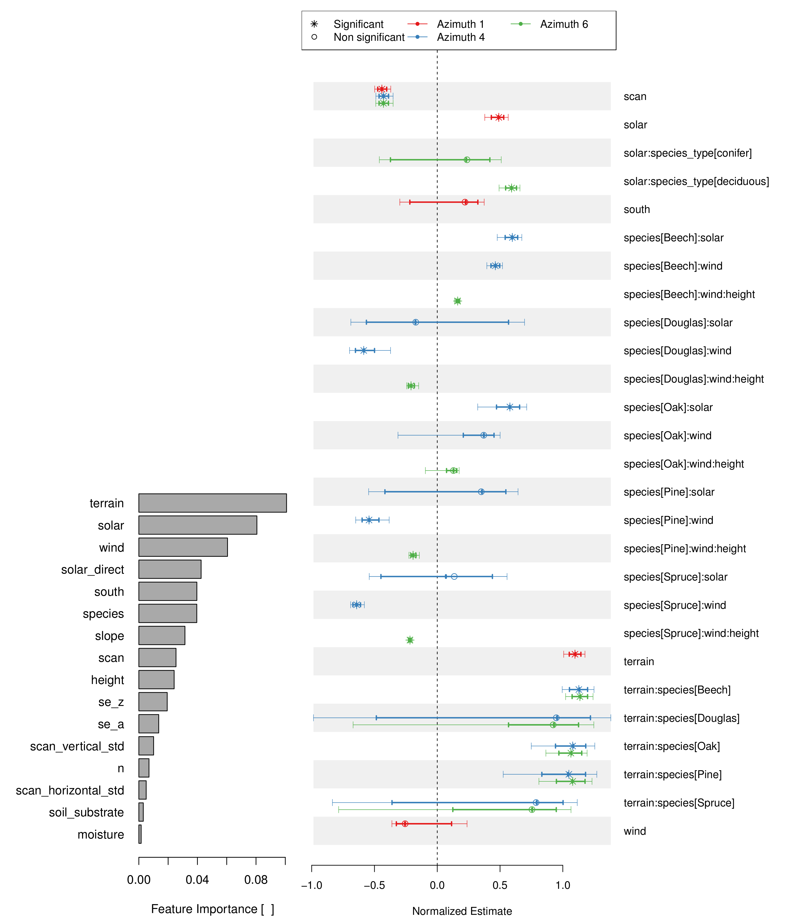
4.5.2. Trunk Orientation
Figure 17 as well as Table 6 and Table 7 illustrate the feature selection procedure for modeling the trunk orientation. The Random Forest regressor achieves an adjusted of about while the circular standard deviation is about 62°. It identifies the terrain and solar—as the composites of the site aspect and the slope inclination, respectively direct solar radiation—as the driving factors for the trunk orientation. It also identifies the wind—as the combination of the prevailing wind direction and speed—and the scan direction as important explanatory variables. Except for the tree species, the non-directed parameters achieve a lower feature importance, while the soil moisture as well as the soil substrate have a minor contribution to the model. With adjusted values ranging from to , as well as circular standard deviations ranging from 76° to 83°, the linear models achieve less accurate results than the Random Forest regressor. But, up to about 19% of the variance can be explained by the linear models.
In accordance with the Random Forest regressor, with up to 14.7% of the variance explained by interactions with the vectors terrain and solar (see Azimuth 6), the linear models identify the aspect as the variable with most explanatory power. As Figure 17 illustrates, the trees tend to lean down-slope, while significant species dependent differences can be found (terrain:species, solar:species). In detail, deciduous trees gain a positive solar coefficient, while the coefficient for conifers does not differ significantly from zero (see solar:species_type). Although a general tendency of the trunk orientation to the South could be found in Section 4.4, the effect is not significant. Also a grouping by tree species (south:species) does not reveal any significant effects. In consequence, the observed South inclination of the trunks (compare Figure 14) is probably the result of the interactions with the site aspect. The high explanatory power of the vectors solar—representing the relative direct solar radiation—and terrain are indicators for the interaction between phototropism and the terrain as the driving factor for the observed South-inclination of the trunks.
With up to 3.2% variance explained, the prevailing wind direction and speed (wind) have a significant species dependent effect on the trunk orientation (wind:species). In particular, conifers tend to lean leeward, while the models imply that beech tend to lean windward.
In accordance with the results of the trunk inclination modeling (Section 4.5.1), the tree height has a significant effect on the trunk orientation. In particular, it intensifies the species depending leeward or windward orientation (wind:species:height) of the trunks.
With 0.8% to 0.9% of variance explained by the vector scan, the LiDAR scan direction has a minor but significant and robust effect on the trunk orientation for all six linear models. The model coefficients imply that the trunk vectors are systematically inclined towards the direction of acquisition. But, this effect might still be an artifact of the systematic scanning pattern.
Table 8 highlights that the explanatory power of the vectors strongly depends on tree species. In particular, with 22.6% of the variance explained, the orientation of deciduous trees can be modeled more accurately than the orientation of the conifers with only 10.7%. In detail, the orientation of the deciduous trees (beech and oak) is driven by interactions with the site aspect resulting in about 20% of the variance explained by terrain:species and solar:species_type, while with about 2% the wind has a minor, but significant contribution.
In contrast, with 11.1% the orientation of the spruce is driven by the interaction of the tree height with wind, while the site aspect has no significant effect. In general, the effect of solar is not significant for conifers, while the terrain is only significant for pine. For Douglas and pine, the interaction of tree height with wind has a considerable effect on the trunk orientation.
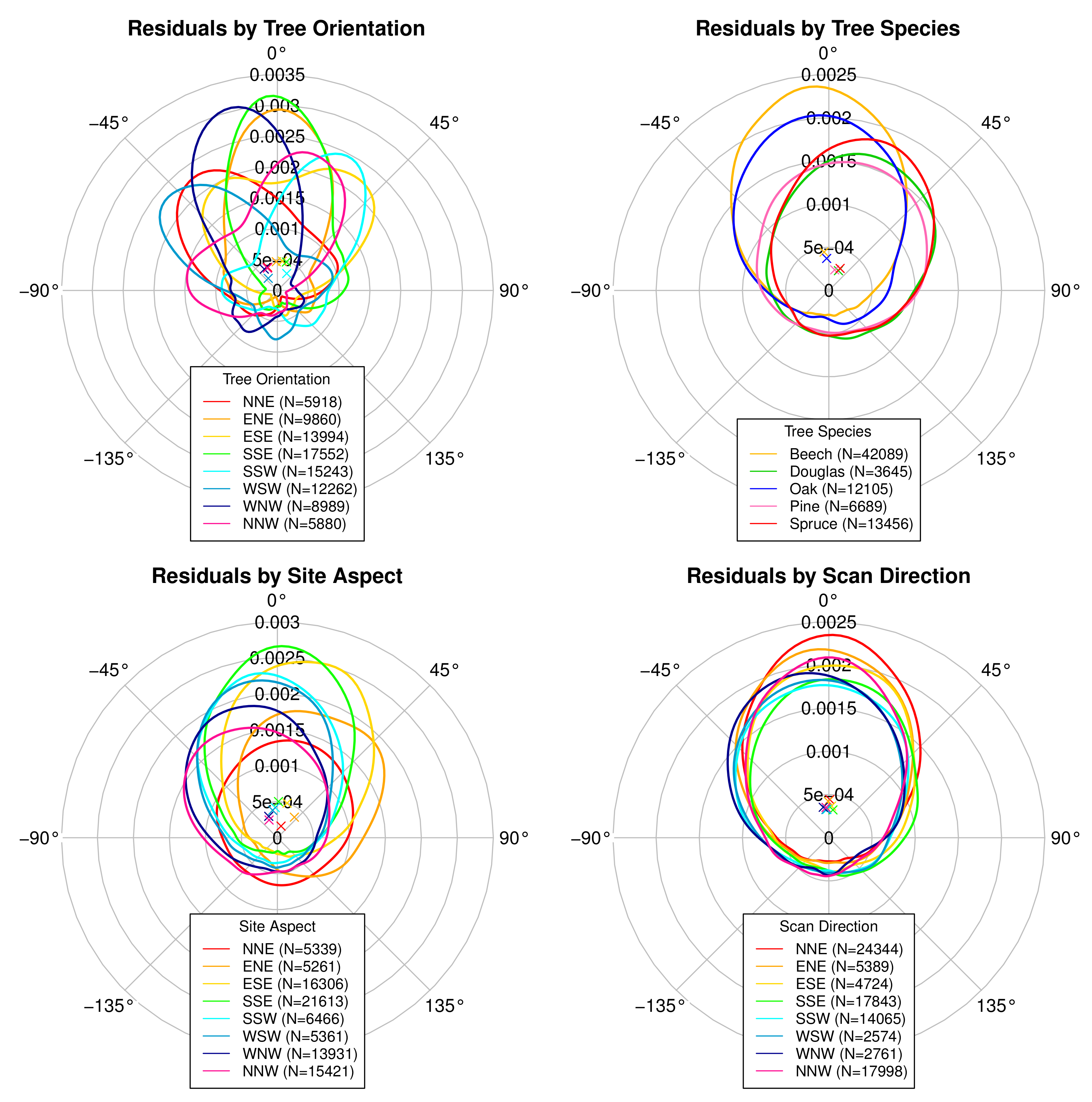
Although the orientation of the trunks has been used to weight the linear equations, Figure 18 reveals that the predicted orientation is not fully independent from the observed orientation . In particular, trunks inclined to the South-South-East and the East-North-East axes show the lowest residuals. In addition, the accuracy of the model depends on the tree species and site aspect, while the effect of the scan direction is minor.
5. Discussion
The given study demonstrates that ALS detected tree trunks show preferred vector orientations (Hypothesis 1). In particular, most of the trunks lean down-slope (Hypothesis 2) and a general tendency to the South can be observed. The linear regression models imply that this interaction is highly species specific (Hypothesis 3) and strongest for sites facing to the South, but diminishes for sites directed away from the sun. Almost 20% of the predicted orientation of the beech is related to the site aspect, compared to about 0% for spruce. These observations are in alignment with the expected species dependent interaction between phototropism and tilted terrains as investigated by Matsuzaki et al. [6]. In the given study, the interaction between the site aspect and the direct solar radiation is suitable to explain the observed South orientation of the trunks.
With 11.1% (spruce), 5.7% (Douglas) and 4.1% (pine) of the variance explained by the interaction between tree species and tree height with the dominant wind direction and speed, the conifers tend to lean leeward (Hypothesis 4). With only 2.0% for beech and 0.6% for oak, this effect is minor for deciduous trees. These results are in alignment with Gardiner et al. [9] and Fourcaud et al. [17], since in particular spruce are highly vulnerable to wind drag due to their compact crown shape and their flat roots. By adaptive growth of the roots [9,13] and reducing the wind-drag by realigning the crown shape, the wind resistance is increased [9,11]. Both effects might cause the observed leeward orientation of the stems.
No significant effect of the soil substrate as well as the soil moisture on the tree inclination can be found in the given study. Since soil characteristics [16] and soil moisture [9,44] have been expected to influence the resistance against toppling of trees, the given results are contrary to Hypothesis 6.
As a confounding variable, the ALS acquisition direction shows a minor, but significant effect on the observed trunk inclination and orientation. Since the systematic West-East flight pattern in combination with the Southeast-Northwest orientation of the mountain range makes an auto-correlation with the preferred South inclination highly probable, no final conclusion on Hypothesis 5 can be drawn in this study.
5.1. Strengths and Limitations
The high uncertainty of ALS detected trunk vectors results in hidden patterns. Even for the significantly inclined trunks, more than half of the observed trunk inclination is associated with attributes expressing the uncertainty of the vectors. As a consequence, a huge number of tree trunks need to be identified to make qualitative statements on the underlying causes for trunk inclination and orientation.
To address this issue, the trunk detection method developed for this study is designed to rapidly identify a majority of doubtless linear structures based on heuristics. Its simplicity allows for a full analysis of the study area covering hundreds of square kilometers within a reasonable amount of time (in the magnitude of several hours). By excluding all trunk vectors with an uncertain orientation, hidden patterns can be revealed. Since the algorithm provides a biased sample of dominant trees—for example, by missing trees of the understory—effects like those postulated by Ishii and Higashi [7] cannot be investigated by this approach. To gain a deeper insight, an accuracy assessment of the trunk detection algorithm and an analysis of the detection rates for different habitats should be applied for future studies. Additionally, in this study the significance of the conclusions is limited to the tree trunks only. Statements on the influence of the underlying causes on the shape and orientation of the tree crowns are inadmissible.
By predicting the trunk orientation using a linear combination of explanatory vectors, qualitative statements on the effect directions can be drawn. The strength of this knowledge-driven approach lies in its simplicity, since the orientation of the trunks is modeled as the sum of the explanatory vectors only. In consequence the effects postulated by Gardiner et al. [9] and Matsuzaki et al. [6] can be empirically confirmed in this study. A limitation of using a linear combination of vectors is given in its inability to describe effects oblique to the vector directions. In consequence such effects can be described by an interaction of the vectors only. To incorporate non linear interaction terms, a detailed prior knowledge on the underlying causes is required. In addition to these conceptual limitations, the ordinary least squares regression cannot achieve the mathematically optimal solution, since the model minimizes the residuals instead of (see Equation (5)).
As an empirical pre-study to investigate the usefulness of ALS data to study the tree trunk inclination and orientation, the input data is not optimal for a detailed thematic analysis. In particular, the geometric resolution of the wind dataset used in this study is much too coarse to inspect the small-scale variation of the wind direction and speed and their effect on the inclination of trees. But, due to the complex interaction between forests and the terrain [9], a sufficient accuracy on the individual tree level might still not be achievable. Due to the low variability of the wind directions in the study area, it might correlate with the trunk orientation by coincidence. Other factors influencing the wind-drag, like the forest structure, tree spacing and site conditions [9] could not be considered in the given study.
The tree species classification map used in the given study shows some weaknesses in the investigated area. In consequence, species dependent effects might have been covered due to miss-classified tree trunks. The explanatory power of the soil moisture is limited due to the spatial resolution of the soil moisture map. Also due to the spatial auto-correlation between slope inclination, soil moisture and tree species, potential effects might have been covered. The soil substrate has not shown any significant effect on the trunk inclination. This is probably caused by the low spatial resolution and the coarse class division, which give poor information on the actual structural integrity of the soils. Again, more suitable input data and a detailed geo-spatial analysis could reveal hidden effects.
Despite the weaknesses of the input data, for the first time—to the knowledge of the authors—the given study can empirically confirm systematic trunk inclination patterns using ALS data. In particular, several hypotheses on the trunk orientation can be addressed. Effects like the species dependent interaction between phototropism in tilted terrains—as postulated by Matsuzaki et al. [6]—can be confirmed.
5.2. Future Research
Having shown that the ALS derived trunk orientations are in alignment with the current state of knowledge on tree inclination, a transfer to other study areas seems promising. Trunk detection might serve as a tool to empirically confirm assumptions on predominant tree orientations on large scales. With more robust detection methods, the number of identified trunks and the accuracy of the trunk vectors may be increased, allowing for more detailed analyses. In general, a focus should be set on the geo-spatial analysis of the trunk inclination and orientation while comparing this information with terrestrial reference data. In this manner, the investigation of the ALS derived trunk inclination and orientation may be used to identify landslide areas and to estimate the potential wind drag to assess the risk of wind throw. In this context, a supplementary detection of fallen trees and the investigation of storm events would provide valuable information.
6. Conclusions
This study has shown that tree trunks detected using airborne laser scanning can provide information on preferred stem inclination angles and directions. Although a significant proportion of the trunk inclination variance is associated with the uncertainty of the fitted trunk vectors, an empirical analysis has shown that the observed orientation of the significantly inclined trunks is in alignment with today’s state of knowledge. In particular, weighted least squares regression models—describing the trunk orientation as a linear combination of directed explanatory variables—have confirmed a highly species specific down-slope inclination of the trunks. While the orientation of beech and oak is dominated by the site aspect—associated with the interaction of phototropism and tilted terrains—the spruce tend to lean leeward. The orientation of the conifers Douglas and pine seems to be driven by both, aspect and wind.
Given these results, the detection of tree trunks using airborne laser scans might be a promising tool to investigate the effect of various influence factors on the tree inclination and orientation. In addition to empirically confirming findings of fundamental research, the presented methods might be used to identify landslides or to address the risk of wind throw on large scales.
Author Contributions
Conceptualization, S.L. and T.U.; methodology, S.L.; software, S.L.; investigation, S.L.; resources, J.S., writing—original draft preparation, S.L.; writing—review and editing, J.S. and T.U.; visualization, S.L.; supervision, T.U.; funding acquisition, S.L. and T.U. All authors have read and agreed to the published version of the manuscript.
Funding
This work has been supported by the European Commission under the grant agreement number 774571 Project PANTHEON.
Acknowledgments
The authors wish to thank the state forest service of Rhineland-Palatinate (Landesforsten RLP) for providing the ecological site classification layers and the state surveying and geoinformation service of Rhineland-Palatinate (LVermGeo) the ALS data.
Conflicts of Interest
The authors declare no conflict of interest. The funders had no role in the design of the study; in the collection, analyses, or interpretation of data; in the writing of the manuscript, or in the decision to publish the results.
Abbreviations
The following abbreviations are used in this manuscript:
| ALS | Airborne Laser Scanning |
| GPS | Global Positioning System |
| IoU | Intersection over Union |
| LiDAR | Light Detection And Ranging |
| LVermGeo | Landesamt für Vermessung und Geobasisinformation Rheinland-Pfalz |
| NNE | North-North-East |
| ENE | East-North-East |
| ESE | East-South-East |
| SSE | South-South-East |
| SSW | South-South-West |
| WSW | West-South-West |
| WNW | West-North-West |
| NNW | North-North-West |
| I | Relative direct solar radiation. |
| Solar declination angle in . | |
| Geographic latitude in . | |
| Hour of the day. | |
| Slope of the surface in . | |
| Site aspect in . | |
| Declination angle . | |
| h | True sun height . |
| Apparent sun height . | |
| DOY | Day of year. |
Appendix A. Solar Radiation
References
- Lamprecht, S.; Stoffels, J.; Dotzler, S.; Haß, E.; Udelhoven, T. aTrunk—An ALS-Based Trunk Detection Algorithm. Remote Sens. 2015, 7, 9975. [Google Scholar] [CrossRef] [Green Version]
- Chen, R.; Rosen, E.; Masson, P.H. Gravitropism in Higher Plants. Plant Physiol. 1999, 120, 343–350. [Google Scholar] [CrossRef] [Green Version]
- Christie, J.M.; Murphy, A.S. Shoot phototropism in higher plants: New light through old concepts. Am. J. Bot. 2013, 100, 35–46. [Google Scholar] [CrossRef]
- Iino, M. Phototropism in higher plants. In Photomovement; Elsevier: Amsterdam, The Netherlands, 2001; pp. 659–811. [Google Scholar] [CrossRef]
- Johns, J.W.; Yost, J.M.; Nicolle, D.; Igic, B.; Ritter, M.K. Worldwide hemisphere-dependent lean in Cook pines. Ecology 2017, 98, 2482–2484. [Google Scholar] [CrossRef] [PubMed] [Green Version]
- Matsuzaki, J.; Masumori, M.; Tange, T. Stem Phototropism of Trees: A Possible Significant Factor in Determining Stem Inclination on Forest Slopes. Ann. Bot. 2006, 98, 573–581. [Google Scholar] [CrossRef] [PubMed] [Green Version]
- Ishii, R.; Higashi, M. Tree coexistence on a slope: An adaptive significance of trunk inclination. Proc. R. Soc. Lond. Ser. B Biol. Sci. 1997, 264, 133–139. [Google Scholar] [CrossRef] [Green Version]
- Wistuba, M.; Malik, I.; Gärtner, H.; Kojs, P.; Owczarek, P. Application of eccentric growth of trees as a tool for landslide analyses: The example of Picea abies Karst. in the Carpathian and Sudeten Mountains (Central Europe). CATENA 2013, 111, 41–55. [Google Scholar] [CrossRef]
- Gardiner, B.; Berry, P.; Moulia, B. Review: Wind impacts on plant growth, mechanics and damage. Plant Sci. 2016, 245, 94–118. [Google Scholar] [CrossRef]
- Schindler, D.; Bauhus, J.; Mayer, H. Wind effects on trees. Eur. J. For. Res. 2011, 131, 159–163. [Google Scholar] [CrossRef] [Green Version]
- Telewski, F.W.; Jaffe, M.J. Thigmomorphogenesis: Field and laboratory studies of Abies fraseri in response to wind or mechanical perturbation. Physiol. Plant. 1986, 66, 211–218. [Google Scholar] [CrossRef]
- Telewski, F.W. Is windswept tree growth negative thigmotropism? Plant Sci. 2012, 184, 20–28. [Google Scholar] [CrossRef] [PubMed]
- Nicoll, B.C.; Ray, D. Adaptive growth of tree root systems in response to wind action and site conditions. Tree Physiol. 1996, 16, 891–898. [Google Scholar] [CrossRef] [PubMed] [Green Version]
- Planck, N.R.V.; MacFarlane, D.W. Branch mass allocation increases wind throw risk for Fagus grandifolia. For. Int. J. For. Res. 2019, 92, 490–499. [Google Scholar] [CrossRef]
- Gardiner, B.; Byrne, K.; Hale, S.; Kamimura, K.; Mitchell, S.J.; Peltola, H.; Ruel, J.C. A review of mechanistic modelling of wind damage risk to forests. Forestry 2008, 81, 447–463. [Google Scholar] [CrossRef] [Green Version]
- Smiley, E.T.; Key, A.; Greco, C. Root barriers and windthrow potential. J. Arboric. 2000, 26, 213–217. [Google Scholar]
- Fourcaud, T.; Ji, J.N.; Zhang, Z.Q.; Stokes, A. Understanding the Impact of Root Morphology on Overturning Mechanisms: A Modelling Approach. Ann. Bot. 2007, 101, 1267–1280. [Google Scholar] [CrossRef] [Green Version]
- Lu, X.; Guo, Q.; Li, W.; Flanagan, J. A bottom-up approach to segment individual deciduous trees using leaf-off lidar point cloud data. ISPRS J. Photogramm. Remote Sens. 2014, 94, 1–12. [Google Scholar] [CrossRef]
- Polewski, P.; Yao, W.; Heurich, M.; Krzystek, P.; Stilla, U. Free shape context descriptors optimized with genetic algorithm for the detection of dead tree trunks in als point clouds. ISPRS Ann. Photogramm. Remote Sens. Spat. Inf. Sci. 2015, 1, 41–48. [Google Scholar] [CrossRef] [Green Version]
- Shendryk, I.; Broich, M.; Tulbure, M.G.; Alexandrov, S.V. Bottom-up delineation of individual trees from full-waveform airborne laser scans in a structurally complex eucalypt forest. Remote Sens. Environ. 2016, 173, 69–83. [Google Scholar] [CrossRef]
- Amiri, N.; Polewski, P.; Yao, W.; Krzystek, P.; Skidmore, A.K. Detection of Single Tree Stems in Forested Areas from High Density Als Point Clouds Using 3D Shape Descriptors. ISPRS Ann. Photogramm. Remote Sens. Spat. Inf. Sci. 2017, IV-2/W4, 35–42. [Google Scholar] [CrossRef] [Green Version]
- Windrim, L.; Bryson, M. Detection, Segmentation, and Model Fitting of Individual Tree Stems from Airborne Laser Scanning of Forests Using Deep Learning. Remote Sens. 2020, 12, 1469. [Google Scholar] [CrossRef]
- Chen, W.; Hu, X.; Chen, W.; Hong, Y.; Yang, M. Airborne LiDAR Remote Sensing for Individual Tree Forest Inventory Using Trunk Detection-Aided Mean Shift Clustering Techniques. Remote Sens. 2018, 10, 1078. [Google Scholar] [CrossRef] [Green Version]
- Zhen, Z.; Quackenbush, L.J.; Zhang, L. Trends in Automatic Individual Tree Crown Detection and Delineation—Evolution of LiDAR Data. Remote Sens. 2016, 8, 333. [Google Scholar] [CrossRef] [Green Version]
- Bucksch, A.; Lindenbergh, R.; Menenti, M. SkelTre. Vis. Comput. 2010, 26, 1283–1300. [Google Scholar] [CrossRef] [Green Version]
- Chen, H.H.; Huang, T.S. A survey of construction and manipulation of octrees. Comput. Vis. Graph. Image Process. 1988, 43, 409–431. [Google Scholar] [CrossRef]
- Reeb, G. Sur les points singuliers d‘une forme de Pfaff compltèment intégrable ou d‘une fonction numérique. C. R. Hebd. Sances Acad. Sci. 1946, 222, 847–849. [Google Scholar]
- Razak, K.A.; Bucksch, A.; Straatsma, M.; Westen, C.J.V.; Bakar, R.A.; de Jong, S.M. High density airborne lidar estimation of disrupted trees induced by landslides. In Proceedings of the 2013 IEEE International Geoscience and Remote Sensing Symposium—IGARSS, Melbourne, Australia, 21–26 July 2013. [Google Scholar] [CrossRef] [Green Version]
- Kini, A.U.; Popescu, S.C. TreeVaW: A Versatile Tool for Analyzing Forest Canopy LIDAR Data: A Preview with an Eye towards Future; ASPRS: Kansas City, MO, USA, 2004. [Google Scholar]
- MUEEF. Daten der Forstlichen Standortkartierung—InGrid-Portal. 2013. Available online: https://www.portalu.rlp.de/trefferanzeige?docuuid=54C251AF-542E-11D7-B776-0002A5CE70F9 (accessed on 23 July 2020).
- Stoffels, J.; Hill, J.; Sachtleber, T.; Mader, S.; Buddenbaum, H.; Stern, O.; Langshausen, J.; Dietz, J.; Ontrup, G. Satellite-Based Derivation of High-Resolution Forest Information Layers for Operational Forest Management. Forests 2015, 6, 1982–2013. [Google Scholar] [CrossRef]
- RIEGL. LMS-Q560. Available online: http://www.riegl.com/uploads/tx_pxpriegldownloads/10_DataSheet_Q560_20-09-2010_01.pdf (accessed on 27 September 2016).
- Lamprecht, S. Pyoints: A Python package for point cloud, voxel and raster processing. J. Open Source Softw. 2019, 4, 990. [Google Scholar] [CrossRef]
- Krähenmann, S.; Walter, A.; Brienen, S.; Imbery, F.; Matzarakis, A. Monthly, daily and hourly grids of 12 commonly used meteorological variables for Germany estimated by the Project TRY Advancement. Theor. Appl. Climatol. 2016. [Google Scholar] [CrossRef]
- Landesamt für Geologie und Bergbau Rheinland-Pfalz. Bodenübersichtskarte 1:200.000 (BÜK200)—CC6302 Trier. 2019. Available online: https://www.lgb-rlp.de/karten-und-produkte/online-karten/online-bodenkarten.html (accessed on 17 December 2019).
- Torr, P.; Zisserman, A. MLESAC: A New Robust Estimator with Application to Estimating Image Geometry. Comput. Vis. Image Underst. 2000, 78, 138–156. [Google Scholar] [CrossRef] [Green Version]
- Cressman, G.P. An Operational Objective Analysis System. Mon. Weather Rev. 1959, 87, 367–374. [Google Scholar] [CrossRef]
- Gassel, A. Beiträge zur Berechnung Solarthermischer und Exergieeffizienter Energiesysteme. Ph.D. Thesis, Fakultät Maschinenwesender Technischen Universität Dresden, Dresden, Germany, 1996. [Google Scholar]
- Sheather, S.J.; Jones, M.C. A Reliable Data-Based Bandwidth Selection Method for Kernel Density Estimation. J. R. Stat. Soc. Ser. B 1991, 53, 683–690. [Google Scholar] [CrossRef]
- Wright, M.N.; Ziegler, A. Ranger: A Fast Implementation of Random Forests for High Dimensional Data in C++ and R. J. Stat. Softw. 2017, 77. [Google Scholar] [CrossRef] [Green Version]
- Mardia, K.V. Statistics of Directional Data; Academic Press: London, UK, 1972. [Google Scholar] [CrossRef]
- Agostinelli, C.; Lund, U. R Package Circular: Circular Statistics (Version 0.4-93); Department of Environmental Sciences, Informatics and Statistics, Ca’ Foscari University: Venice, Italy; Department of Statistics, California Polytechnic State University: San Luis Obispo, CA, USA, 2017. [Google Scholar]
- Jammalamadaka, S.R.; SenGupta, A. Topics in Circular Statistics; World Scientific: Singapore, 2001. [Google Scholar] [CrossRef]
- Gardiner, B.; Schuck, A.; Schelhaas, M.; Orazio, C.; Blennow, K.; Nicoll, B. (Eds.) Living with Storm Damage to Forests; Number 3 in What Science Can Tell Us; European Forest Institute: Joensuu, Finland, 2013. [Google Scholar]
Figure 1.
Overview map of the study area Hunsrück-Hochwald National Park.

Figure 2.
Tree species distribution within the study area Hunsrück-Hochwald National Park (left) and digital elevation model derived from ALS point clouds (right). The ALS point clouds have been provided by LVermGeo, while the tree species classification is the result of Stoffels et al. [31]. Coordinates are shown in ETRS89/UTM system (EPSG 25832).

Figure 3.
ALS flight lines and study area Hunsrück-Hochwald National Park. Coordinates are shown in ETRS89/UTM system (EPSG 25832).
Figure 3.
ALS flight lines and study area Hunsrück-Hochwald National Park. Coordinates are shown in ETRS89/UTM system (EPSG 25832).

Figure 4.
Fifteen year average (1989–2012) of the wind direction and wind speed in the study area (left) and wind rose diagram of the same area and time window (right). Both figures have been derived from daily wind models provided by Krähenmann et al. [34]. Coordinates are shown in ETRS89/UTM system (EPSG 25832).

Figure 5.
Dominating soil substrates (left) and soil moisture regimes (right) in the study area. Coordinates are shown in ETRS89/UTM system (EPSG 25832).
Figure 5.
Dominating soil substrates (left) and soil moisture regimes (right) in the study area. Coordinates are shown in ETRS89/UTM system (EPSG 25832).

Figure 6.
A duplicate point filter with filtering radius R is applied to points associated with vegetation (left). The resulting filtered point cloud serves as the input for a density filter (center). Points with more than 3 neighboring points within radius R are omitted. Working principle of the vertical line filter with maximum horizontal distance R and z-axis scaled by factor 4 (right).

Figure 7.
The filtered point cloud serves as the input for the clustering algorithm (left). A point is assigned to the most frequent class of its neighboring points within radius 1.5R. To prefer linear structures, the z-axis is scaled by factor . A regression vector is fitted to each trunk cluster (center). Implausible vectors are omitted from further analyses. Each regression vector defines a local coordinate system, with axes v, z and a (right). The black dots represent the trunk points, while the red dot corresponds to the trunk root.

Figure 8.
Relative direct solar radiation depending on site aspect for differing site slopes at solar noon in summer at a geographic latitude of 50°N.
Figure 8.
Relative direct solar radiation depending on site aspect for differing site slopes at solar noon in summer at a geographic latitude of 50°N.

Figure 9.
Density plots of the trunk inclination (left) and trunk orientation (right) grouped by differing significance levels of the trunk inclination. For each group, the mean trunk orientation is marked with a cross.
Figure 9.
Density plots of the trunk inclination (left) and trunk orientation (right) grouped by differing significance levels of the trunk inclination. For each group, the mean trunk orientation is marked with a cross.

Figure 10.
Site aspect in relation to slope (left), scan compass direction in relation to the scan zenith angle (center) and trunk orientation in relation to the trunk inclination (right).
Figure 10.
Site aspect in relation to slope (left), scan compass direction in relation to the scan zenith angle (center) and trunk orientation in relation to the trunk inclination (right).

Figure 11.
Density of the tree trunks for the explanatory variables wind direction (left), site aspect (center) and scan direction (right) grouped by tree species.
Figure 11.
Density of the tree trunks for the explanatory variables wind direction (left), site aspect (center) and scan direction (right) grouped by tree species.

Figure 12.
Pearson’s product moment correlation coefficients for scalar variables (left) and directed variables (right).
Figure 12.
Pearson’s product moment correlation coefficients for scalar variables (left) and directed variables (right).

Figure 13.
Influence of the tree species on the trunk inclination (left) and trunk orientation (right). The deciduous trees tend to lean to the South, while the conifers tend to lean to the East. The orientation follows the site aspect, while a general trend to the South can be observed.
Figure 13.
Influence of the tree species on the trunk inclination (left) and trunk orientation (right). The deciduous trees tend to lean to the South, while the conifers tend to lean to the East. The orientation follows the site aspect, while a general trend to the South can be observed.

Figure 14.
Influence of the slope on the tree inclination (left) and effect of the aspect on the trunk orientation (right).
Figure 14.
Influence of the slope on the tree inclination (left) and effect of the aspect on the trunk orientation (right).

Figure 15.
Effect of the site aspect on differing tree species.

Figure 16.
Permutation feature importance of the Random Forest regressor (left) and regression coefficients of selected linear trunk inclination models (right). The coefficients are scaled by to display them in the same plot. The given 98% and 80% confidence intervals are based on bootstrapping.
Figure 16.
Permutation feature importance of the Random Forest regressor (left) and regression coefficients of selected linear trunk inclination models (right). The coefficients are scaled by to display them in the same plot. The given 98% and 80% confidence intervals are based on bootstrapping.

Figure 17.
Permutation feature importance of the Random Forest regressor (left) and regression coefficients of selected linear trunk orientation models (right). The coefficients are scaled by to display them in the same plot. The given 98% and 80% confidence intervals are based on bootstrapping.
Figure 17.
Permutation feature importance of the Random Forest regressor (left) and regression coefficients of selected linear trunk orientation models (right). The coefficients are scaled by to display them in the same plot. The given 98% and 80% confidence intervals are based on bootstrapping.

Figure 18.
Residuals of the linear trunk orientation model Azimuth 6 depending on observed trunk orientation (top-left), tree species (top-right), site aspect (bottom-left) and scan direction (bottom-right).
Figure 18.
Residuals of the linear trunk orientation model Azimuth 6 depending on observed trunk orientation (top-left), tree species (top-right), site aspect (bottom-left) and scan direction (bottom-right).


Table 1.
Comparison of surface area with the amount of detected stems.
| Beech | Douglas | Oak | Pine | Spruce | |
|---|---|---|---|---|---|
| Area of classification layer | 36.8% | 11.4% | 13.9% | 9.8% | 28.1% |
| Number of detected stems | 40.7% | 6.5% | 11.5% | 8.3% | 32.9% |
Table 2.
Distribution of soil properties by tree species.
| Tree Species | ||||||
|---|---|---|---|---|---|---|
| Soil Property | Beech | Douglas | Oak | Pine | Spruce | |
| Soil substrate | Quarzite | 73.5% | 72.2% | 70.7% | 68.8% | 67.4% |
| Quarzite & Shales | 26.2% | 27.5% | 27.8% | 30.5% | 32.4% | |
| Shales | 0.3% | 0.3% | 1.5% | 0.6% | 0.2% | |
| Soil moisture | dry | 3.1% | 5.4% | 10.0% | 5.6% | 3.7% |
| moist | 82.2% | 84.3% | 85.8% | 83.4% | 81.8% | |
| very moist | 14.7% | 10.3% | 4.2% | 11.0% | 14.4% | |
Table 3.
Inclination and orientation of the significantly inclined trunks for different species.
| Beech | Douglas | Oak | Pine | Spruce | Average | |
|---|---|---|---|---|---|---|
| ± | ± | ± | ± | ± | ± | |
| ± | ± | ± | ± | ± | ± |
Table 4.
Amount of trees inclined with a specific explanatory variable for different groups.
| Inclination Direction | |||||
|---|---|---|---|---|---|
| Group | Southward | Down-Slope | Leeward | in Scan Direction | |
| Species | Beech | 70.8% | 77.2% | 39.9% | 40.3% |
| Douglas | 56.2% | 60.5% | 61.0% | 50.4% | |
| Oak | 65.5% | 74.1% | 44.5% | 42.9% | |
| Pine | 54.5% | 63.4% | 58.8% | 43.1% | |
| Spruce | 53.6% | 51.8% | 67.5% | 53.7% | |
| Species Type | Conifer | 54.3% | 56.3% | 64.1% | 50.2% |
| Deciduous | 69.6% | 76.5% | 40.9% | 40.9% | |
| Root System | Flat | 53.6% | 51.8% | 67.5% | 53.7% |
| Heart | 69.7% | 75.9% | 41.6% | 41.1% | |
| Tap | 61.6% | 70.3% | 49.6% | 43.0% | |
| Total | 66.0% | 71.3% | 46.8% | 43.3% | |
Table 5.
Total and partial per regression coefficient of the linear trunk inclination models. Coefficients significantly different from zero are marked in bold. Significant inter group differences are marked in italics.
Table 5.
Total and partial per regression coefficient of the linear trunk inclination models. Coefficients significantly different from zero are marked in bold. Significant inter group differences are marked in italics.
| Zenith 1 | Zenith 2 | Zenith 3 | Zenith 4 | Zenith 5 | Zenith 6 | |
|---|---|---|---|---|---|---|
| (Intercept) | 0.010 | 0.000 | 0.000 | 0.096 | ||
| se_z | 0.308 | 0.314 | 0.312 | 0.312 | 0.311 | 0.307 |
| se_a | 0.020 | 0.021 | 0.025 | 0.025 | 0.025 | 0.024 |
| n | 0.002 | 0.003 | ||||
| scan_horizontal_std | 0.009 | 0.010 | 0.011 | 0.011 | 0.011 | 0.010 |
| scan_vertical_std | 0.000 | 0.000 | ||||
| scan_zenith | 0.001 | 0.001 | ||||
| wind_mean_speed | 0.000 | 0.000 | ||||
| solar_direct | 0.001 | 0.001 | ||||
| height | 0.076 | 0.067 | 0.074 | 0.074 | 0.075 | 0.083 |
| slope | 0.018 | 0.013 | 0.013 | 0.013 | 0.013 | 0.018 |
| species:moisture:soil_substrate | 0.004 | 0.004 | ||||
| species | 0.001 | 0.098 | ||||
| moisture | 0.000 | |||||
| soil_substrate | 0.001 | |||||
| Total | 0.573 | 0.590 | 0.586 | 0.581 | 0.578 | 0.570 |
Table 6.
Average explained variance per regression coefficient for the linear trunk orientation models. Coefficients significantly different from zero are marked in bold. Significant inter group differences are marked in italics. Measures are based on the training data set .
Table 6.
Average explained variance per regression coefficient for the linear trunk orientation models. Coefficients significantly different from zero are marked in bold. Significant inter group differences are marked in italics. Measures are based on the training data set .
| Azimuth 1 | Azimuth 2 | Azimuth 3 | Azimuth 4 | Azimuth 5 | Azimuth 6 | |
|---|---|---|---|---|---|---|
| terrain | 8.9% | |||||
| terrain:species | 8.5% | 8.3% | 8.4% | 8.5% | 8.5% | |
| solar | 4.1% | |||||
| solar:species | 6.2% | 6.3% | 6.3% | 6.1% | ||
| solar:species_type | 6.2% | |||||
| wind | −0.1% | |||||
| wind:species | 2.9% | 3.2% | 3.2% | |||
| wind:species:height | 3.6% | 3.6% | ||||
| south | 0.3% | −0.1% | ||||
| south:species | 0.5% | |||||
| scan | 0.9% | 0.8% | 0.8% | 0.8% | 0.8% | 0.8% |
| Total | 14.0% | 18.8% | 18.5% | 18.6% | 19.1% | 19.1% |
Table 7.
Accuracy metrics of the trunk orientation prediction (coefficient of determination , mean angular deviation , circular standard deviation and the amount of trunks inclined with the model ). The metrics are based on the training data set .
Table 7.
Accuracy metrics of the trunk orientation prediction (coefficient of determination , mean angular deviation , circular standard deviation and the amount of trunks inclined with the model ). The metrics are based on the training data set .
| RF | Azimuth 1 | Azimuth 2 | Azimuth 3 | Azimuth 4 | Azimuth 5 | Azimuth 6 | |
|---|---|---|---|---|---|---|---|
| 82.8% | 71.9% | 74.7% | 75.0% | 75.0% | 75.3% | 75.3% |
Table 8.
Average explained variance per regression coefficient of the regression model Azimuth 6 depending on tree species. The measures are based on the validation data set . If applicable, coefficients significantly different from zero are highlighted in bold.
Table 8.
Average explained variance per regression coefficient of the regression model Azimuth 6 depending on tree species. The measures are based on the validation data set . If applicable, coefficients significantly different from zero are highlighted in bold.
| Beech | Douglas | Oak | Pine | Spruce | Conifer | Deciduous | Total | |
|---|---|---|---|---|---|---|---|---|
| terrain:species | 11.4% | 3.2% | 9.8% | 5.7% | 0.3% | 2.2% | 11.1% | 8.4% |
| solar:species_type | 9.0% | 0.2% | 8.0% | 0.3% | 0.0% | 0.1% | 8.8% | 6.1% |
| wind:species:height | 2.0% | 5.7% | 0.6% | 4.1% | 11.1% | 8.3% | 1.7% | 3.7% |
| scan | 1.2% | 0.0% | 0.8% | 0.8% | −0.4% | −0.0% | 1.1% | 0.8% |
| Total | 23.7% | 9.1% | 19.2% | 10.9% | 11.0% | 10.7% | 22.7% | 19.0% |
Publisher’s Note: MDPI stays neutral with regard to jurisdictional claims in published maps and institutional affiliations. |
© 2020 by the authors. Licensee MDPI, Basel, Switzerland. This article is an open access article distributed under the terms and conditions of the Creative Commons Attribution (CC BY) license (http://creativecommons.org/licenses/by/4.0/).
Share and Cite
MDPI and ACS Style
Lamprecht, S.; Stoffels, J.; Udelhoven, T. ALS as Tool to Study Preferred Stem Inclination Directions. Remote Sens. 2020, 12, 3744. https://0-doi-org.brum.beds.ac.uk/10.3390/rs12223744
AMA Style
Lamprecht S, Stoffels J, Udelhoven T. ALS as Tool to Study Preferred Stem Inclination Directions. Remote Sensing. 2020; 12(22):3744. https://0-doi-org.brum.beds.ac.uk/10.3390/rs12223744
Chicago/Turabian StyleLamprecht, Sebastian, Johannes Stoffels, and Thomas Udelhoven. 2020. "ALS as Tool to Study Preferred Stem Inclination Directions" Remote Sensing 12, no. 22: 3744. https://0-doi-org.brum.beds.ac.uk/10.3390/rs12223744
Note that from the first issue of 2016, this journal uses article numbers instead of page numbers. See further details here.