Article

Adjudicating Perspectives on Forest Structure: How Do Airborne, Terrestrial, and Mobile Lidar-Derived Estimates Compare?

by
Jonathon J. Donager
1,
Andrew J. Sánchez Meador
2,* and
Ryan C. Blackburn
3
1
Ecological Restoration Institute, Northern Arizona University, Flagstaff, AZ 86011, USA
2
Ecological Restoration Institute and School of Forestry, Northern Arizona University, Flagstaff, AZ 86011, USA
3
School of Forestry, Northern Arizona University, Flagstaff, AZ 86011, USA
*
Author to whom correspondence should be addressed.
Remote Sens. 2021, 13(12), 2297; https://0-doi-org.brum.beds.ac.uk/10.3390/rs13122297
Submission received: 22 April 2021 / Revised: 3 June 2021 / Accepted: 9 June 2021 / Published: 11 June 2021
(This article belongs to the Special Issue Feature Paper Special Issue on Forest Remote Sensing)

Abstract

:
Applications of lidar in ecosystem conservation and management continue to expand as technology has rapidly evolved. An accounting of relative accuracy and errors among lidar platforms within a range of forest types and structural configurations was needed. Within a ponderosa pine forest in northern Arizona, we compare vegetation attributes at the tree-, plot-, and stand-scales derived from three lidar platforms: fixed-wing airborne (ALS), fixed-location terrestrial (TLS), and hand-held mobile laser scanning (MLS). We present a methodology to segment individual trees from TLS and MLS datasets, incorporating eigen-value and density metrics to locate trees, then assigning point returns to trees using a graph-theory shortest-path approach. Overall, we found MLS consistently provided more accurate structural metrics at the tree- (e.g., mean absolute error for DBH in cm was 4.8, 5.0, and 9.1 for MLS, TLS and ALS, respectively) and plot-scale (e.g., R2 for field observed and lidar-derived basal area, m2 ha−1, was 0.986, 0.974, and 0.851 for MLS, TLS, and ALS, respectively) as compared to ALS and TLS. While TLS data produced estimates similar to MLS, attributes derived from TLS often underpredicted structural values due to occlusion. Additionally, ALS data provided accurate estimates of tree height for larger trees, yet consistently missed and underpredicted small trees (≤35 cm). MLS produced accurate estimates of canopy cover and landscape metrics up to 50 m from plot center. TLS tended to underpredict both canopy cover and patch metrics with constant bias due to occlusion. Taking full advantage of minimal occlusion effects, MLS data consistently provided the best individual tree and plot-based metrics, with ALS providing the best estimates for volume, biomass, and canopy cover. Overall, we found MLS data logistically simple, quickly acquirable, and accurate for small area inventories, assessments, and monitoring activities. We suggest further work exploring the active use of MLS for forest monitoring and inventory.

Graphical Abstract

1. Introduction

Successful forest conservation, management, and restoration require detailed information on forest structure and composition, which are vital decision-making components and modeling inputs. This information has been commonly used to assess current condition, compare management outcomes, and in the case of forest restoration, monitor the success or failure of moving a degraded ecosystem towards recovery. Efforts to quantify ecological patterns and processes typically necessitate precise data on the amount and distribution of biotic and abiotic resources, estimates of how resources may change over time, and assessments of disturbance [1]. These activities often require costly and resource-intensive spatially explicit data, and to be useful for conservation and management of forested ecosystems, need to include site-specific information on vegetation pattern (sizes and species), fuel conditions and arrangement, wildlife habitat suitability, and operational condition [2,3,4].
However, compounding costs, reduced workforce capacity, and increasing scales for planning and implementation often make information obtained from direct field measurements (i.e., plot samples) inadequate, incomplete, or altogether impossible despite being the standard for field data collection. Remote sensing platforms have become increasingly popular with resource managers, which can push the limits of information acquisition when describing forest resources at landscape-scales [5,6,7,8,9,10]. Chief among these tools has been lidar, with newer technologies such as terrestrial (TLS) and mobile laser scanning (MLS) being increasingly investigated for applications in forest ecosystems [11,12,13,14,15].
The restoration and management of ecologically sensitive frequent fire forests of the southwestern United States requires the ability to make rapid assessments prior to treatment and frequent monitoring of post-treatment ecological outcomes. Mobile laser scanner systems offer a powerful tool to ease the time and labor demands of traditional plot-based sampling while potentially providing accurate and highly precise estimates of basic forest structural conditions [12,13]. While fixed-wing airborne laser scanning (ALS) platforms have been commonplace for decades, more recently, terrestrial and mobile lidar systems have been investigated for characterizing forest structure, as their higher point densities allow for more detailed and robust extraction of structural attributes, sub-canopy occlusion of smaller trees and other ecologically important species can be reduced, and their data can be collected more frequently than airborne systems [13,16,17,18,19,20,21]. While the absolute positional error of points collected by MLS was typically less precise than TLS due to the propagation of positioning errors accumulated during scan registrations (e.g., see Figure 1), MLS made use of localization algorithms (e.g., SLAM; Simultaneous Localization and Mapping), which enabled accurate positioning of the scanner in vegetated environments where GNSS and GPS signals were typically hindered by dense canopies and the movement of MLS may have reduced overall occlusion [13,15,22].
Terrestrial and mobile lidar may be particularly effective for monitoring changes in forest ecosystems, especially where species composition and structural complexity were relatively simple and where periodic or time-sensitive measurements were needed [21,23,24]. Historically, individual tree segmentation algorithms applied to lidar datasets have relied on the forest canopy to initiate and delineate trees. However, this process becomes complicated where interlocking crowns exist, an ecologically relevant and common occurrence, and tends to miss trees which do not extend into the dominant crown layer. Recent years have seen new approaches for delineating individual trees, including layer stacking methods [25] and graph-based segmentation approaches [26,27,28].
One of the primary necessities to accelerating ecological restoration in forested ecosystems, especially in the frequent fire forests of the western US, has been the accurate and timely assessment of forest structure. However, information concerning effectiveness of mobile lidar systems for monitoring and rapid assessment of forest conditions were lacking. Stemming from this need, we sought to understand how forest structural estimates resulting from mobile and terrestrial scanning systems compare to more established estimates coming from aerial lidar and traditional field-based forest monitoring plots. More specifically, in this study, we compare methodologies for assessing (a) individual-tree, (b) stand-level, and (c) canopy cover and landscape metrics attributes derived from rasterized canopy height models among datasets obtained from ALS, TLS, and MLS platforms across a range of forest conditions in a ponderosa pine forest of northern Arizona, USA. Resulting tree and forest characteristics were compared to assess relative accuracies across scale.

2. Materials and Methods
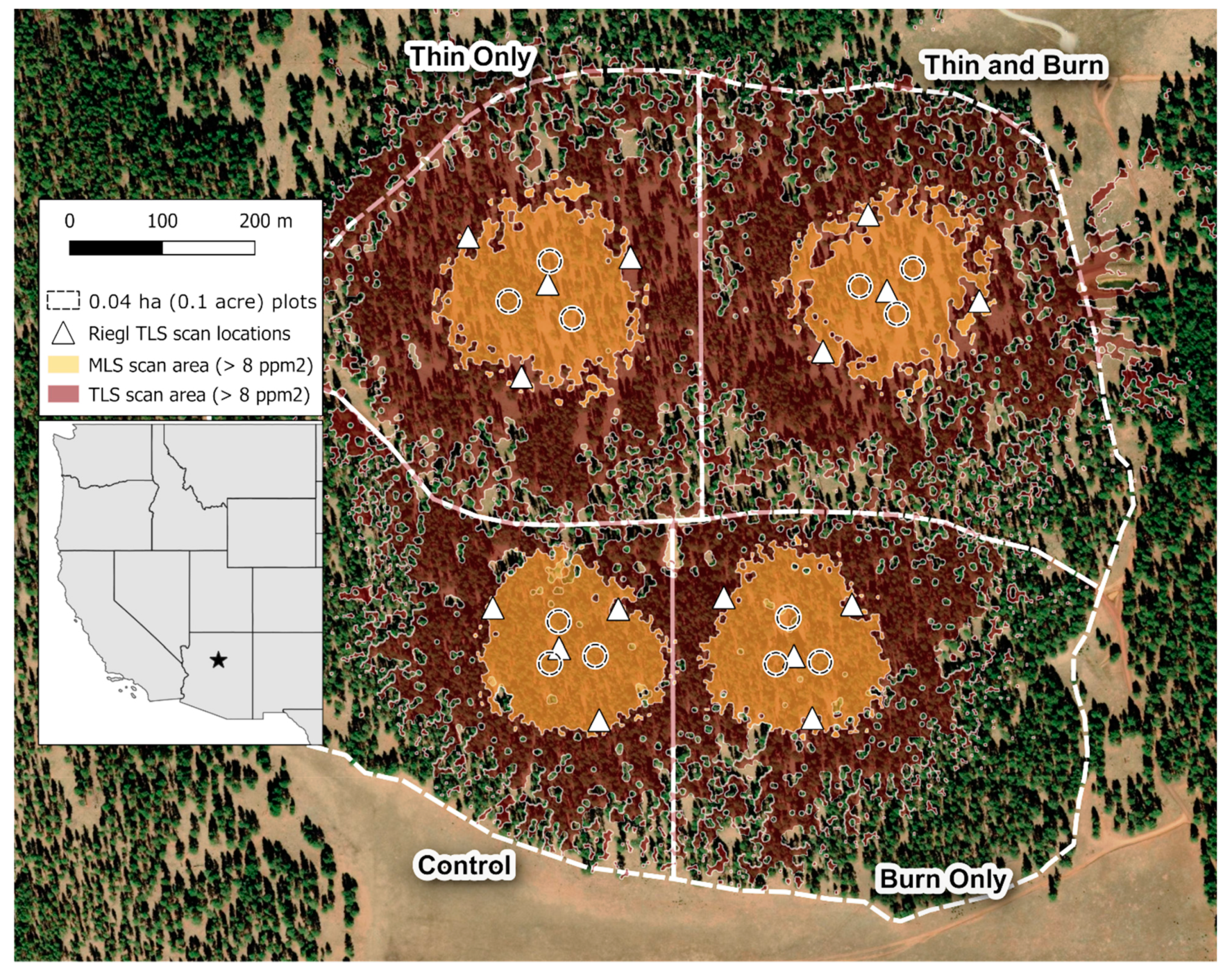
2.1. Study Site

For this study, we focused on a pure ponderosa pine (Pinus ponderosa) forest near Flagstaff, AZ where we could make use of previously collected ALS and TLS lidar datasets (Figure 2) [18]. These sites were managed by the US Forest Service as part of the “Fire and Fire Surrogate” study network [29] with original treatment objectives including fuels reductions [30]. In brief, the study design presented an ideal tree density gradient resulting from four treatments: thinning from below (thin-only), broadcast burning (burn-only), a combination of thinning from below with subsequent broadcast burning (thin-and-burn), and an untreated control (Figure 2). Mean elevation was 2270 m with slight variation in slope (<5%) and aspect. Mean annual precipitation was 546 mm, which falls as rain during monsoons (July–September) and snow in the winter months [31]. Average yearly temperature extremes ranged from −12 to 28 °C [30].

2.2. Field Data Collection

Field data for twelve sample plots were collected in summer 2020 with plot locations placed to maximize existing TLS scan coverage and stratified along a tree density gradient. We used circular plots (0.04 ha) and centers were recorded with a Trimble Geo7X GPS and differentially corrected using Trimble’s Pathfinder Office. For all trees with a measurable diameter at breast height (DBH; measured at 1.37 m above ground level), location was mapped using a LaserTech MapStar TruAngle angle encoder and TruPulse 200X laser rangefinder (±0.05° and ±4 cm accuracy, respectively), and DBH, height, height to the base of the live crown, species, and condition (alive or dead) were recorded. Summaries of the field data were shown in Table 1. Data consisted of 209 ponderosa pine trees on 12 sample plots, with densities ranging from open conditions (25 trees ha−1) to dense, closed canopy, conditions (1361 trees ha−1). While denser conditions for contemporary forest have been reported for nearby sites, e.g., [32], the conditions observed were a unique opportunity to explore patterns of tree detection and estimation accuracy for typical ponderosa pine forest conditions across western USA.

2.3. Lidar Data Acquisitions and Processing

The ALS data used in this study was collected in August of 2018 to QL1 specifications (a minimum point density of 8 points per m2). ALS point density across our site was 19.8 points per m2. A Riegl VQ 1560i lidar sensor was flown at an altitude of 1800 m, collecting up to 1.3 million points per second. The data were processed to industry specification, including bare earth model generation, point classification, and cleaning of the resulting point cloud data. The vertical accuracy was reported at 0.085 m for non-vegetated elevation and 0.14 m for vegetated elevation.
Mobile lidar data was collected using a GeoSlam Zeb Horizon (www.geoslam.com/us/zeb-horizon/; accessed on 30 March 2021) handheld mobile laser scanner in May 2020. The scanner was initiated at each plot center and walked in a flower petal design with three “petals” radiating from center towards north (0° heading), southeast (120° heading), and southwest (240° heading) with a final ring around the 0.04 ha plot. The scanner employs a Velodyne VLP-16 scanner on a rotating mount, resulting in a scan acquisition with a nearly total field of view around the device collecting 300,000 points per second. While the device is constantly collecting information once initiated, individual scans are tied together using GeoSlam’s proprietary SLAM algorithm, resulting in a unified point cloud of the scan area. The resulting point cloud contains a large amount of positional “noise” (compared to ALS and TLS), largely stemming from the Velodyne scanner and the SLAM algorithm, with a resulting point accuracy of 1–3 cm.
As stated in the previous section, we designed this study to coincide with an existing terrestrial lidar dataset employed in a previous study [18] where the authors examined occlusion and effective distances for terrestrial scanning in forested environments. The scanner, a Riegl VZ-1000 is a survey-grade terrestrial scanner with a range of over 1400 m and integrated inclination sensors for real-time orientation and can acquire up to 122,000 points per second and has a 360° horizontal and 100° vertical field of view. All scans were conducted between August 2015 and March 2016. Individual scan locations were established between 70 and 100 m from a central scan and registered to one another using Riegl’s proprietary software.
We used ALS data as positional reference for the mobile and terrestrial lidar datasets by manually shifting (rotation and translation) point clouds to ALS data, then using an iterative closest point algorithm to further match our lidar datasets. In this way, trees segmented from one dataset represent the same trees segmented in another, and thus our analysis produced fair comparisons. For all datasets, we classified ground points using the cloth simulation filter method [33] and normalized the point clouds. We performed minimal noise filtering to remove spurious high and low noise from the point clouds.

2.4. Tree-Level Comparisons

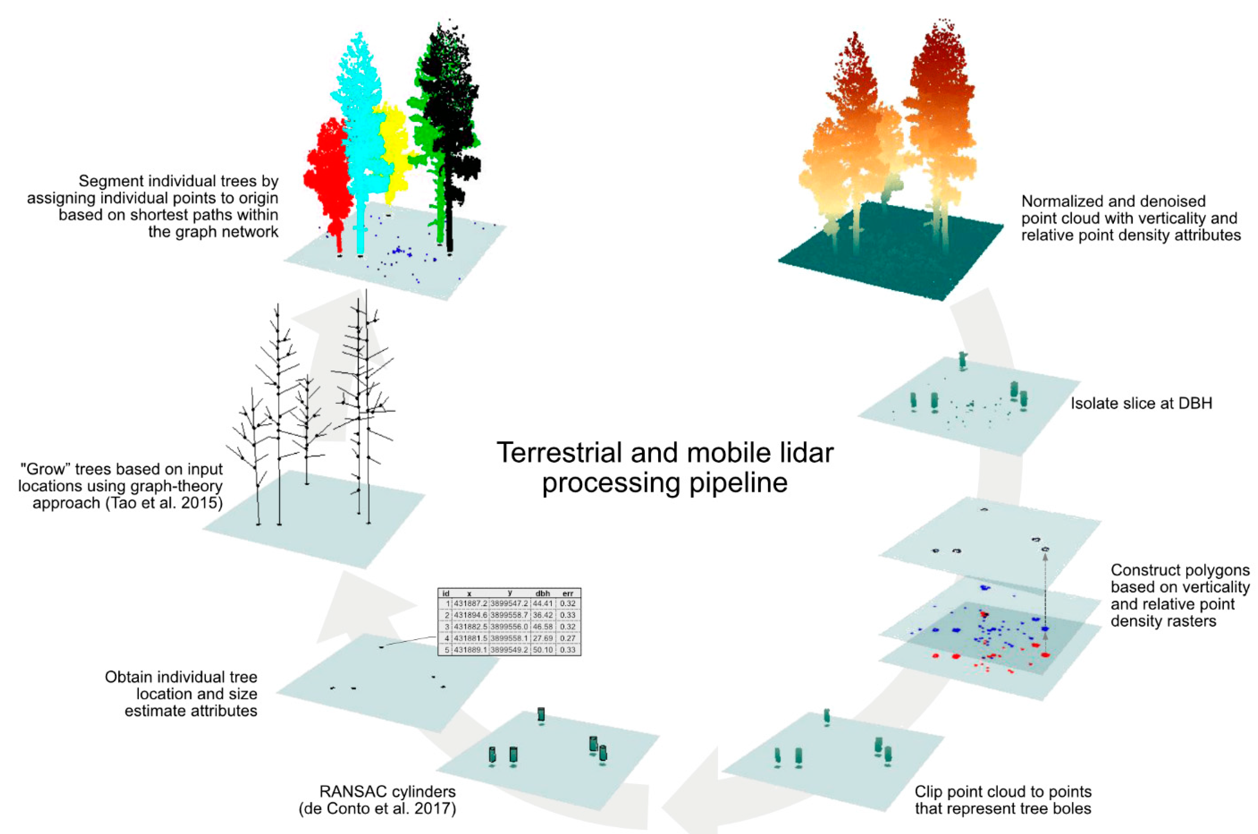
2.4.1. Segmentation Approaches

We investigated multiple individual tree segmentation algorithms appropriate to each dataset by employing methods that utilized the point cloud in a manner consistent with the mode of acquisition for each lidar platform. All point clouds were first normalized to remove the effects of elevation and topography after identifying likely ground points using the cloth simulation filter algorithm [33] as implemented in the lidR package (v3.0.4) [34] in the R (v4.0.3; R Core Team 2020) environment. For the airborne lidar dataset, we investigated top-down approaches as the sensor directly observes the top of the canopy and more accurately describe canopy height. Specifically, we tested two commonly used tree segmentation approaches implemented in the lidR package: a seeded region-growing approach [35] and a region growing approach which works within the point cloud [36]. From our initial testing, we found the Dalponte and Coomes [35] algorithm more accurately segmented trees from our ALS dataset and so we performed the full analysis with this method alone. We obtained DBH for each ALS segmented tree using a nonlinear least squares regression model based on the observed relationship between height and DBH for 2116 ponderosa pine trees in Arizona [37]. Terrestrial and mobile lidar platforms produce less reliable canopy heights than ALS data as they operate below canopy, however they are able to directly observe tree boles. For these platforms, we developed a custom methodology which made use of eigen-values calculated within point neighborhoods, a measure of relative neighborhood point density, random sample consensus (RANSAC) cylinder fitting and a shortest path graph theory approach to delineating individual trees using a set of custom functions in conjunction with the TreeLS package (v2.0.2) [38].
For terrestrial and mobile lidar datasets, our analysis approach (Figure 3) determined tree locations and estimates of DBH by rasterizing individual point cloud values of relative neighborhood density (0.3 and 1 m radius) and verticality within a slice of the normalized point cloud around breast height (1.34 m). We then defined threshold values to classify the resulting rasters and created unique polygons from the resulting classified raster. These point-density and verticality polygons were selected by their intersection with one another, resulting in a final set of polygons which were used to clip out regions of the point cloud that were most likely to represent tree boles. We then used a random sample consensus (RANSAC) cylinder fitting algorithm from the TreeLS package (v2.0.2) [38] to identify individual bole points. Cylinder centers and radius were used as inputs to an individual tree segmentation approach which follows ecological principles for “growing” trees based on these input locations in a graph-theory approach inspired by work of [27]. Point coordinates were linked together based on proximity and turned into a graph object, using the estimated tree bole locations as origin points, connecting individual points back to those origins based on shortest paths within the graph network, and finally those points were assigned to unique tree identifiers based on the bole coordinate to which they were connected. The R scripts, released under GPL-3.0 license, used for processing and performing individual tree segmentations (Figure 3), can be found at https://github.com/bi0m3trics/spanner, accessed on 30 March 2021.

2.4.2. Tree-Matching and Error Estimation

After segmentation, each segmented tree set (ALS, MLS, TLS) was matched to the corresponding field measured trees. To begin the matching process, a 3 m radius buffer was constructed around each field measured tree to find potential candidate trees from lidar segmentations. We allowed for a larger buffer for taller trees by adding the tree height divided by the mean height of all field trees. The remaining segmented trees were then given a matching error to select the most similar tree. Differences in segmentation approaches (i.e., treetops for airborne vs. boles for terrestrial) created the need to use different attributes when estimating matching errors. For ALS, differences in height and location were used based on the top-down approach of segmentation (Equation (1)). ALS segmented trees with differences in heights greater than 2 m were excluded from matching until the next iteration (i.e., the next field tree was matched). Additionally, we weighted the field tree by their associated basal area to give more weight to larger trees.
( h t d i f f + l o c d i f f ) B A
For MLS and TLS, differences in DBH and location were used based on the bottom-up approach of segmentation (Equation (2)). The corresponding matched trees (segmented and field-measured) were then removed from the tree sets and the matching process was repeated
d b h d i f f + l o c d i f f

2.4.3. Tree-Level Attributes

Tree matching allowed us to quantify tree-level differences in characteristics and detection, omission, and commission rates for each lidar scanning platform. Within each plot, detection rates were calculated as the number of matched trees divided by the number of field measured trees. Omission and commission rates were calculated as the number of unmatched field measured trees (omission) or the number of unmatched segmented trees (commission) divided by the total number of field measured trees within a plot. Tree location, height, and DBH were then compared between matched trees. For height and DBH, mean absolute error (MAE) and root mean squared error (RMSE) as a percent of the plot mean were calculated. Location differences were investigated visually. Kruskal–Wallis tests were used to test differences between matched tree attributes.

2.5. Stand-Level and Landscape Metrics Comparisons

2.5.1. Stand-Level Attributes

Tree density, basal area, volume, aboveground biomass, and diameter distributions were quantified by following traditional forest inventory estimation procedures. Volume was estimated from DBH and total height using the United States Department of Agriculture, Forest Service’s National Volume Estimator Library (NVEL; https://www.fs.fed.us/forestmanagement/products/measurement/volume/nvel/; accessed on 20 March 2021) and the Flewelling 2-point profile model [39]. Total aboveground, oven-dry biomass was estimated from DBH using the component biomass equations provided [40] and summed for the individual tree. Dunn’s tests were used to test differences among plot-level platform-derived values and Kolmogorov–Smirnov tests were used to test differences in tree size-class distributions.

2.5.2. Canopy Cover and Landscape Metrics

We built binary classifications of canopy cover from canopy height models calculated from normalized point clouds at each plot location buffered by 100 m to ensure we captured the gradient of canopy cover classification accuracy. Canopy height models were built at 0.33 m resolution and using a function to replace each single point with a circle of 8 points to better represent the footprint of an individual laser pulse [34]. Due to the point density, we used a subcircle radius size of 0.2 m for ALS data and 0.1 m for MLS and TLS data. Canopy cover was defined as canopy height greater than DBH and we compared mean canopy cover within 1 m annular cylinders originating at plot center and extending to 100 m distance. Using the resulting canopy cover comparisons as a guide, we examined patch size and density landscape metrics for each plot using extents of 5 to 50 m buffered distance from plot center. Landscape metrics were calculated from the resulting clipped canopy cover rasters using the landscapemetrics package (v1.5.1) [41] and Kruskal–Wallis rank sum tests were performed to test for differences.

3. Results

3.1. Tree-Level Comparisons

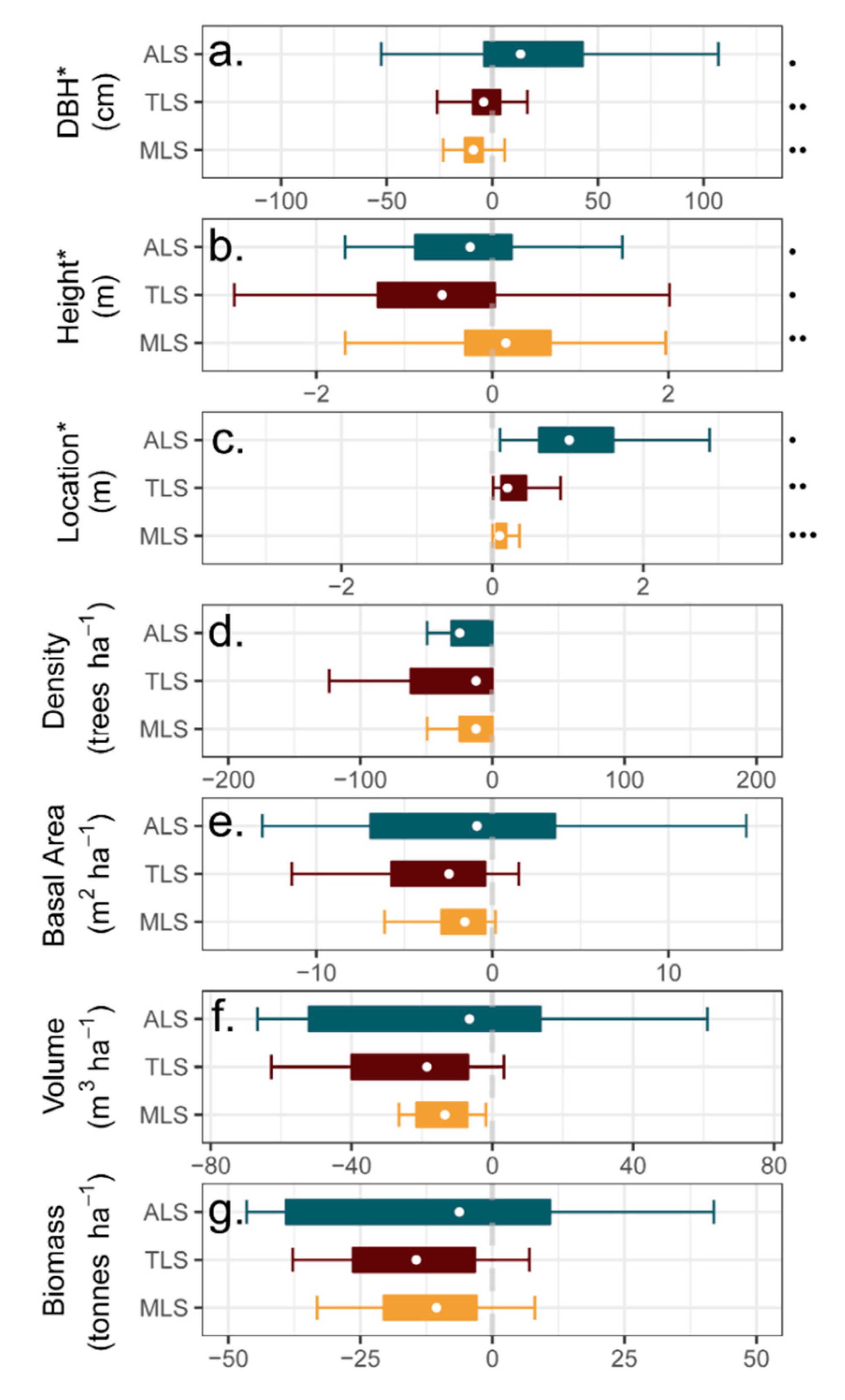
3.1.1. Individual Tree Size and Location

Kruskal–Wallis rank sum tests showed significant difference by platform between prediction errors for DBH, height and tree location (Figure 4). The post-hoc Dunn’s tests revealed that overpredictions of DBH by ALS were significantly larger than that of TLS and MLS (Figure 4a), for which the latter were not significantly different. Mean absolute error (MAE) for DBH was lowest for MLS (4.8 cm) and only slightly smaller than TLS (5.0 cm; Table 2). However, ALS predictions of DBH, which had to be derived from tree height, were found to be significantly higher with MAE of 9.1 cm (Table 2). Both ALS and TLS tended to underpredict total tree height (Figure 4b), and with corresponding MAEs of 0.7 m and 2.2 m. MLS was found to over predict height with a MAE of 1.3 meters. Tree locations from MLS exhibited the smallest prediction errors (Figure 4c), followed by those obtained by TLS and ALS, and all were significantly different with means under 1.27 m (Figure 4c). The same patterns were true for percent RMSE (Table 2).In examining individual-tree field observations versus platform-specific estimates (Figure 5), all three datasets produced estimates which appeared to overestimate smaller tree diameters (Figure 5a–c). MLS and TLS tended to overestimate DBH of trees smaller than 25 cm but produced more accurate estimates of DBH for trees greater than 25 cm (Figure 5b,c). Estimates of DBH derived from the ALS data displayed much greater variation, but in general, exhibited overpredictions of DBH among smaller trees and underprediction of DBH among larger trees (Figure 5a). Individual tree height was most accurately predicted by ALS, with very little variation from field measurements of tree height (Figure 5d). However, our displayed results do not emphasize that numerous trees went undetected using ALS (n = 103), as smaller and sub-dominant trees were often occluded from ALS. For example, no heights below 7 m were reported when summarizing ALS-derived tree heights (Figure 5d). MLS-derived tree heights tended towards overestimation as compared to both field measurements and TLS-derived estimates (Figure 5e,f), with the latter providing estimates that were lower than their observed height for several trees 15–25 m in height (Figure 5f). Tree locations varied the least among segmentations from MLS data using the workflow we developed (Figure 5g–i). While some increased error was apparent among trees further from plot center, MLS data exhibited a predominately uniform distribution of low individual-tree location errors (Figure 5h).

3.1.2. Plot-Level Observations

As summarized at the plot-level, MLS data in concert with the methods we developed for this study provided the most consistent segmentation of trees among plots with nearly 95% detection (Table 2). An important yet often unreported result was the fact that we were alerted to data entry errors (i.e., the absence of six trees among two plots in our field data) when making comparisons to MLS-based individual-tree segmentations. Stemming from tree segmentation, rates of omission (field trees not detected) and commission (field trees falsely created) were lowest from MLS outputs (Table 2). TLS plot-level estimates were less accurate at nearly 87% detection rate, but TLS had nearly double the rate of omission compared to MLS estimates. ALS estimates were much lower than those obtained from our terrestrially-based datasets, with a mean detection rate of 68.3% (Figure 2). Mean rates of omission and commission were generally large for ALS (31.7%, 53.2%), with commission on one plot exceeding the number of trees observed (Table 2).

3.2. Stand-Level and Landscape Metric Comparisons

3.2.1. Stand-Level Attributes

Unlike patterns observed for predictions of individual trees, Kruskal–Wallis rank sum tests did not reveal any significant difference by platform between prediction errors for plot-level attributes of tree density, basal area, volume and aboveground biomass (Figure 6d–g). However, MLS-derived predictions of tree density were consistent with field-based estimates (R2 = 0.99) and displayed very little deviation from field-based estimates (Figure 6a). Both TLS- and ALS-derived estimates tended to underestimate with increasing tree density (Figure 6a). Basal area predictions were nearly equally predicted by MLS (R2 = 0.73) and TLS datasets (R2 = 0.74), with TLS data tending to underpredict with increasing field-observed basal area (Figure 6b). ALS-derived estimates varied with respect to corresponding field observations, producing least correlated estimates for both tree density (R2 = 0.91) and basal area (R2 = 0.56).
Total stem wood volume exhibited the highest correlation with MLS-derived predictions (R2 = 0.68), which tended to increasingly underpredict with greater volume (Figure 6c). The same pattern was observed for TLS-derived predictions (Figure 6c). While agreement in ALS predictions fell close to the 1:1 line, plot-level comparisons were highly variable (Figure 6c). Estimates of aboveground biomass were also largely similar when predicted by MLS- (R2 = 0.66) and TLS-derived (R2 = 0.67) datasets, while TLS-derived estimates became increasing dissimilar with increasing biomass (Figure 6d). ALS-based predictions were highly variable relative to field observations.
Comparisons of diameter distributions (by 5 cm classes) revealed various overall patterns, and all lidar datasets struggled to adequately represent the smallest (<10 cm) diameter classes (Figure 6e). Two-sample Kolmogorov–Smirnov Tests revealed the following: (1) the shape of the MLS and TLS diameter distributions did not significantly differ from the field-observed distribution shape; (2) MLS and TLS did not significantly differ from one another; and (3) both MLS and TLS differed significantly from the ALS distribution shape, which also differed significantly from the field-observed distribution shape. Under visual inspection, the MLS-derived diameter distribution tended to overpredict among the mid-sized classes and slightly underpredict among the largest-sized classes. The TLS-based estimates failed to capture the magnitude of the 10–15 cm diameter class, but otherwise adequately approximated the distribution of field observations (Figure 6e). Lastly, the diameter distribution derived from ALS performed poorly at capturing the lower end of the diameter distribution and grossly overpredicted among the larger-sized diameter classes (Figure 6e) with a threshold occurring around 40 cm DBH.

3.2.2. Canopy Cover

Differences in mean canopy cover derived from MLS data were nearly identical to that of ALS canopy cover (Figure 7a) up to and including a radial distance of 26 m from plot center (0.21 ha or 0.5 ac). Canopy cover differences from ALS continued to decline slowly to radial distances of approximately 40 m, after which differences from ALS increased. TLS differences in canopy cover declined gradually across the 100-m radial extent from plot center but were consistently underpredicted (as compared to ALS estimates). At approximately 50 m in radial distance from plot center, MLS estimates were comparable with TLS estimates of canopy cover (Figure 7a), after which MLS estimates underpredicted. Kruskal–Wallis rank sum tests of differences revealed that TLS estimates of canopy cover were not significantly different from ALS at buffered distances up to 98 m, while MLS-derived estimates of canopy cover were not significantly different up to buffer distances of 55 m (Figure 7a).

3.2.3. Landscape Metrics

Comparisons of landscape metrics (mean and standard deviation in patch area and patch density) displayed consistent patterns among the lidar datasets (Figure 7b–d). Mean and standard deviation of patch area were consistently higher for ALS data values than those obtained from MLS or TLS (Figure 7c,d). Patch density displayed the opposite pattern (Figure 7b) and estimates changed very little for extents beyond 0.13 ha. Based on Kruskal–Wallis rank sum tests of differences (Figure 7), MLS was not significantly different among all extents examined for patch metrics. However, TLS patch metrics showed significant differences for extents of 0.13 ha and greater for patch density and patch area. Neither MLS nor TLS derived estimates of the standard deviation in patch area were significantly different among the extents examined.

4. Discussion

MLS proved to be a useful tool for rapid assessment and monitoring across a range of forest conditions in a ponderosa pine forest of northern Arizona, USA. Lower accuracies found for our ALS and TLS estimates illustrate the problem created by occlusion [18,42]. Mobile systems overcome this issue by incorporating distance measurements from many views during data collection, meaning occlusion from any single look angle can be overcome by additional look angles [13,15]. Furthermore, the logistics of implementing mobile lidar data collection can be much simpler than other lidar platforms. For instance, our scan time ranged from three to five minutes per plot, and assuming SLAM processing could have taken place in parallel, it would have been reasonable to have scanned and processed all twelve plots within a few hours. The mobile platform was hand-held, meaning it could produce scans from a perspective where a person might walk and collect data, and this could be done very fast. While there was no need to extensively plan and orient fixed scan locations to minimize the effects of occlusion, as with TLS acquisitions [18], considerations of potential occlusion still need to be accounted for when utilizing MLS. Lastly, we emphasize the fact that terrestrially-based scanners (MLS and TLS) capture data from the ground, which can provide benefits over ALS when the scale of inquiry was individual- to stand-scale, such as more accurate representation of tree size classes.
Though terrestrial-based scanners provided large benefits over ALS, occlusion and noise within TLS and MLS point clouds, respectively, impact their abilities to describe forest structure attributes accurately. Inherent to SLAM processing due to accumulated small registration errors, MLS data tend to be “noisier” than fixed location TLS data, resulting in a more “fuzzy” point cloud [13,43]. However, our work suggests that with minimal effort to remove the noise, the resulting data perform well in both identifying trees and deriving attributes for those trees. Due to our need to use existing TLS scans, our TLS data exhibited a range of occlusion that could have been reduced with a different arrangement of scan locations. Specifically, portions of tree canopies and small to large sections of individual trees were missing from our data, which led to greater underestimation for most structural metrics.
ALS-based products commonly take advantage of allometric relationships or imputation to estimate forest structure, e.g., [44,45]. While ALS easily facilitated large area coverages and commonly estimated individual tree heights (as well as canopy-related attributes) accurately, ALS also displayed the highest omission and DBH estimation errors, with the latter likely resulting from variability in allometric relationships [42,46]. Given these limitations and our study’s forest structure, ALS poorly described the full gradient of individual tree- to stand-level structural conditions. This lack of adequately representing structural condition was most evident in when examining tree diameter distributions, but can also be seen in the inaccuracies reported for stand volume and biomass. Developing increasingly accurate allometric relationships from terrestrially based data could further capture variability in tree growth forms [20] and potentially improve predictions.
Our tree detection and size errors results compared well with recent studies making use of terrestrially-based lidar systems for forest inventories, including estimates of individual tree height. Comparable studies examining individual tree diameters extracted from MLS and TLS datasets often yield between 1 and 5 cm RMSE, and commonly between 3 and 4 cm [15,21,43,47]. Estimates of tree height from terrestrially-based lidar datasets vary considerably, but generally tend to underpredict [14,15,21]. We were surprised at the generally low RMSE of tree heights obtained with our MLS dataset, which compared well to ALS errors in tree height.
The lack of tools for easily processing terrestrially-collected lidar datasets in an automated fashion targeting conservation and management applications quickly became apparent in our work. While individual trees and corresponding bole sizes were readily apparent by the authors within the resulting MLS and TLS datasets, segmentation approaches either missed trees entirely or aggregated/produced trees much larger than reported by field observations. In general, we found that traditional segmentation approaches, such as canopy height model-based methods and methods using local height maxima for tree locations, performed rather poorly despite the relatively open forest conditions encountered in this study. For example, it is a common practice to directly extract individual tree heights from canopy height models, yet this approach is largely inadequate when sub-dominant canopy layers exist within a forests’ structure, and dense conditions can commonly make it unclear which heights relate to which trees. A recently developed layer stacking methodology [25], theoretically applicable to below-canopy lidar collection, still tended to not capture small diameter trees. As a result, it was necessary to develop methods for better identifying tree locations and performing segmentations in accordance with tree locations observed from below the canopy (i.e., DBH locations). We thus developed eigen-value based rasterization methods to identify tree boles and a segmentation approach which follows ecological principles [27,48,49].
While we endeavored to incorporate a gradient of forest structure conditions commonly found in Southwestern ponderosa pine forests, we were limited by the availability of coincident lidar datasets for the study. While ALS data coverage within the region continues to increase, areas with TLS datasets were very limited and thus why we chose our study site. While this site does provide a large range of forest structural conditions, the study design was also limited by the types of treatments that were originally implemented, as well as the lack of other gradient types, such as climate, soil type, number of canopy strata, or species mixtures. However, this site was typical of large swaths of ponderosa forests across the Southwest. Finally, placement of the TLS scan locations was determined by a previous study seeking to understand how to optimize scan locations within a gradient of forest conditions [18], not to scan multiple 0.04 ha plots. However, such a scan configuration would be typical of real-world TLS applications [17,50].
The MLS data we derived exceeded our expectations and this same collection and processing methodology could be adapted and used in other forest systems. While the authors have no doubt that some of the findings in this study would hold true for different forest types (e.g., airborne platforms would produce the best individual-tree height and canopy cover estimates, terrestrial platforms would produce the best individual-tree location and diameter estimates, and MLS and TLS would outperform ALS in estimating stand-level estimates but are limited in application scale), MLS is a relatively new technology and more research is needed in other ecosystem types. Additionally, efforts to expand and improve the processing algorithms available for terrestrially-based forest lidar datasets are needed; for example, studies exploring the use of a greater number of decomposed eigenvalue metrics calculated at several scales may allow our methodology to better discriminate woody tree boles and tree locations. The structured walk we developed for this study and other 0.04 ha plots worked well in terms of acquiring even data coverage and we plan to experiment with other forms of structured walks for different sizes and shapes of study areas.

5. Conclusions

Effective forest conservation, management, and restoration require a timely assessment of vegetation and forest conditions. ALS data were undoubtedly useful over large areas, but generally only provide insights into structural conditions covered by the dominant canopy and largest trees (i.e., as seen from above), commonly missing the lower end of the size class distribution or vegetation smaller in stature. While collecting TLS data can provide more accurate information with a “bottom up” perspective, the inherent structure of most forests produces particularly challenging conditions for how TLS may “see” the forest, as rates of occlusion or missing data quickly increase with forest density. Mobile systems are uniquely situated in that they are logistically fast and simple to operate, while providing detailed information consistent with how humans view the forest. The ability to quickly mobilize MLS data acquisition both pre- and post-treatment mean MLS data products could be produced quickly to provide time-sensitive insight into adaptive and multi-resource conservation and management. While landscape-scale data cannot be efficiently produced with MLS, it can be easily paired with other datasets, be it ALS data or satellite imagery, to provide location-specific and detailed information. Furthermore, MLS systems can be operated by a single person with minimal logistic planning and expense. The accuracy of our MLS derivatives exceeded our expectations, producing estimates well within the error constraints typically expected for vegetation inventory and monitoring guidelines and consistent with other studies around the world. We expect that we will see the eventual adoption of these technologies throughout resource conservation, management, and restoration practices in the very near future.

Author Contributions

Conceptualization, A.J.S.M. and J.J.D.; methodology, A.J.S.M., J.J.D., and R.C.B.; software, A.J.S.M., J.J.D., and R.C.B.; formal analysis, A.J.S.M., J.J.D., and R.C.B.; investigation, A.J.S.M. and J.J.D.; resources, A.J.S.M.; data curation, A.J.S.M.; writing—original draft preparation, J.J.D. and A.J.S.M.; writing—review and editing, J.J.D., A.J.S.M., and R.C.B.; visualization, A.J.S.M. and J.J.D.; supervision, A.J.S.M.; project administration, A.J.S.M. All authors have read and agreed to the published version of the manuscript.

Funding

This research received no external funding.

Data Availability Statement

The get_raster_eigen_treelocs and segment_graph functions used in this study are available within the spanner package at https://github.com/bi0m3trics/spanner; accessed on 30 March 2021. The version (1.0.0) described in this paper and associated mobile lidar scanning (MLS) data are archived at using Zenodo at http://0-doi-org.brum.beds.ac.uk/10.5281/zenodo.4624277; accessed on 30 March 2021. The terrestrial laser scanning (TLS) data from Donager et al. (2018) are available at https://www.sciencebase.gov/catalog/item/5b85cbaee4b0702d0e77a46b; accessed on 30 March 2021. The airborne laser scanning (ALS) data are available via the U.S. Geological Survey’s National Map Viewer, referencing the “USGS Lidar Point Cloud AZ VerdeKaibab B1 2018” acquisition at https://viewer.nationalmap.gov; accessed on 30 March 2021.

Acknowledgments

We thank United States Geological Survey personnel for their help in collecting the Riegl terrestrial lidar data; the United State Department of Agriculture Forest Service for collection and providing access to the airborne lidar data; Northern Arizona University’s (NAU) Research Equipment Acquisition Program (REAP) for funding the purchase the mobile lidar scanner (MLS); and NAU’s Ecological Restoration Institute for assistance in collecting the MLS data. We specifically thank Joel Sankey and Merideth Reiser for assistance in collecting lidar and field data.

Conflicts of Interest

The authors declare no conflict of interest.

References

  1. Jensen, M.E.; Bourgeron, P.S. A Guidebook for Integrated Ecological Assessments; Springer Science and Business Media LLC: Berlin/Heidelberg, Germany, 2001. [Google Scholar]
  2. Wulder, M.A.; Bater, C.W.; Coops, N.; Hilker, T.; White, J. The role of LiDAR in sustainable forest management. For. Chron. 2008, 84, 807–826. [Google Scholar] [CrossRef] [Green Version]
  3. Stanturf, J.A.; Palik, B.J.; Dumroese, R.K. Contemporary forest restoration: A review emphasizing function. For. Ecol. Manag. 2014, 331, 292–323. [Google Scholar] [CrossRef]
  4. Pettorelli, N.; Laurance, W.F.; O’Brien, T.G.; Wegmann, M.; Nagendra, H.; Turner, W. Satellite remote sensing for applied ecologists: Opportunities and challenges. J. Appl. Ecol. 2014, 51, 839–848. [Google Scholar] [CrossRef]
  5. Boyd, D.S.; Danson, F. Satellite remote sensing of forest resources: Three decades of research development. Prog. Phys. Geogr. Earth Environ. 2005, 29, 1–26. [Google Scholar] [CrossRef]
  6. Hudak, A.T.; Haren, A.T.; Crookston, N.L.; Liebermann, R.J.; Ohmann, J.L. Imputing Forest Structure Attributes from Stand Inventory and Remotely Sensed Data in Western Oregon, USA. For. Sci. 2014, 60, 253–269. [Google Scholar] [CrossRef] [Green Version]
  7. Hansen, E.H.; Gobakken, T.; Bollandsås, O.M.; Zahabu, E.; Næsset, E. Modeling Aboveground Biomass in Dense Tropical Submontane Rainforest Using Airborne Laser Scanner Data. Remote Sens. 2015, 7, 788–807. [Google Scholar] [CrossRef] [Green Version]
  8. Zhang, J.; Hu, J.; Lian, J.; Fan, Z.; Ouyang, X.; Ye, W. Seeing the forest from drones: Testing the potential of lightweight drones as a tool for long-term forest monitoring. Biol. Conserv. 2016, 198, 60–69. [Google Scholar] [CrossRef]
  9. Price, B.; Waser, L.; Wang, Z.; Marty, M.; Ginzler, C.; Zellweger, F. Predicting biomass dynamics at the national extent from digital aerial photogrammetry. Int. J. Appl. Earth Obs. Geoinf. 2020, 90, 102116. [Google Scholar] [CrossRef]
  10. Tang, X.; Hutyra, L.R.; Arévalo, P.; Baccini, A.; Woodcock, C.E.; Olofsson, P. Spatiotemporal tracking of carbon emissions and uptake using time series analysis of Landsat data: A spatially explicit carbon bookkeeping model. Sci. Total. Environ. 2020, 720, 137409. [Google Scholar] [CrossRef]
  11. Vauhkonen, J.; Maltamo, M.; McRoberts, R.E.; Næsset, E. Introduction to Forestry Applications of Airborne Laser Scanning; Springer Science and Business Media LLC: Berlin/Heidelberg, Germany, 2014; Volume 27, pp. 1–16. [Google Scholar]
  12. Bauwens, S.; Bartholomeus, H.; Calders, K.; Lejeune, P. Forest Inventory with Terrestrial LiDAR: A Comparison of Static and Hand-Held Mobile Laser Scanning. Forests 2016, 7, 127. [Google Scholar] [CrossRef] [Green Version]
  13. Chen, S.; Liu, H.; Feng, Z.; Shen, C.; Chen, P. Applicability of personal laser scanning in forestry inventory. PLoS ONE 2019, 14, e0211392. [Google Scholar] [CrossRef]
  14. Liang, X.; Kankare, V.; Hyyppä, J.; Wang, Y.; Kukko, A.; Haggrén, H.; Yu, X.; Kaartinen, H.; Jaakkola, A.; Guan, F.; et al. Terrestrial laser scanning in forest inventories. ISPRS J. Photogramm. Remote Sens. 2016, 115, 63–77. [Google Scholar] [CrossRef]
  15. Hyyppä, E.; Yu, X.; Kaartinen, H.; Hakala, T.; Kukko, A.; Vastaranta, M.; Hyyppä, J. Comparison of Backpack, Handheld, Under-Canopy UAV, and Above-Canopy UAV Laser Scanning for Field Reference Data Collection in Boreal Forests. Remote Sens. 2020, 12, 3327. [Google Scholar] [CrossRef]
  16. Marselis, S.M.; Yebra, M.; Jovanovic, T.; Van Dijk, A.I. Deriving comprehensive forest structure information from mobile laser scanning observations using automated point cloud classification. Environ. Model. Softw. 2016, 82, 142–151. [Google Scholar] [CrossRef]
  17. Liang, X.; Hyyppä, J.; Kaartinen, H.; Lehtomäki, M.; Pyörälä, J.; Pfeifer, N.; Holopainen, M.; Brolly, G.; Francesco, P.; Hackenberg, J.; et al. International benchmarking of terrestrial laser scanning approaches for forest inventories. ISPRS J. Photogramm. Remote Sens. 2018, 144, 137–179. [Google Scholar] [CrossRef]
  18. Donager, J.J.; Sankey, T.T.; Sankey, J.B.; Meador, A.J.S.; Springer, A.E.; Bailey, J.D. Examining Forest Structure with Terrestrial Lidar: Suggestions and Novel Techniques Based on Comparisons Between Scanners and Forest Treatments. Earth Space Sci. 2018, 5, 753–776. [Google Scholar] [CrossRef] [Green Version]
  19. Del Perugia, B.; Giannetti, F.; Chirici, G.; Travaglini, D. Influence of Scan Density on the Estimation of Single-Tree Attributes by Hand-Held Mobile Laser Scanning. Forests 2019, 10, 277. [Google Scholar] [CrossRef] [Green Version]
  20. Disney, M. Terrestrial Li DAR: A three-dimensional revolution in how we look at trees. New Phytol. 2018, 222, 1736–1741. [Google Scholar] [CrossRef] [Green Version]
  21. Calders, K.; Adams, J.; Armston, J.; Bartholomeus, H.; Bauwens, S.; Bentley, L.P.; Chave, J.; Danson, F.M.; Demol, M.; Disney, M.; et al. Terrestrial laser scanning in forest ecology: Expanding the horizon. Remote Sens. Environ. 2020, 251, 112102. [Google Scholar] [CrossRef]
  22. Cabo, C.; Del Pozo, S.; Rodríguez-Gonzálvez, P.; Ordóñez, C.; González-Aguilera, D. Comparing Terrestrial Laser Scanning (TLS) and Wearable Laser Scanning (WLS) for Individual Tree Modeling at Plot Level. Remote Sens. 2018, 10, 540. [Google Scholar] [CrossRef] [Green Version]
  23. Dassot, M.; Constant, T.; Fournier, M. The use of terrestrial LiDAR technology in forest science: Application fields, benefits and challenges. Ann. For. Sci. 2011, 68, 959–974. [Google Scholar] [CrossRef] [Green Version]
  24. Newnham, G.J.; Armston, J.D.; Calders, K.; Disney, M.; Lovell, J.L.; Schaaf, C.B.; Strahler, A.H.; Danson, F.M. Terrestrial Laser Scanning for Plot-Scale Forest Measurement. Curr. For. Rep. 2015, 1, 239–251. [Google Scholar] [CrossRef] [Green Version]
  25. Ayrey, E.; Fraver, S.; Kershaw, J.A., Jr.; Kenefic, L.S.; Hayes, D.; Weiskittel, A.R.; Roth, B.E. Layer Stacking: A Novel Algorithm for Individual Forest Tree Segmentation from LiDAR Point Clouds. Can. J. Remote Sens. 2017, 43, 16–27. [Google Scholar] [CrossRef]
  26. Strîmbu, V.F.; Strîmbu, B.M. A graph-based segmentation algorithm for tree crown extraction using airborne LiDAR data. ISPRS J. Photogramm. Remote Sens. 2015, 104, 30–43. [Google Scholar] [CrossRef] [Green Version]
  27. Tao, S.; Wu, F.; Guo, Q.; Wang, Y.; Li, W.; Xue, B.; Hu, X.; Li, P.; Tian, D.; Li, C.; et al. Segmenting tree crowns from terrestrial and mobile LiDAR data by exploring ecological theories. ISPRS J. Photogramm. Remote Sens. 2015, 110, 66–76. [Google Scholar] [CrossRef] [Green Version]
  28. Williams, J.; Schönlieb, C.-B.; Swinfield, T.; Lee, J.; Cai, X.; Qie, L.; Coomes, D.A. 3D Segmentation of Trees Through a Flexible Multiclass Graph Cut Algorithm. IEEE Trans. Geosci. Remote Sens. 2019, 58, 754–776. [Google Scholar] [CrossRef]
  29. Schwilk, D.; Keeley, J.; Knapp, E.E.; Mciver, J.; Bailey, J.; Fettig, C.; Fiedler, C.; Harrod, R.; Moghaddas, J.J.; Outcalt, K.; et al. The National Fire and Fire Surrogate Study: Effects of fuel re-duction methods on forest vegetation structure and fuels. Ecol. Appl. 2009, 19, 285–304. [Google Scholar] [CrossRef]
  30. Faiella, S.M.; Bailey, J.D. Fluctuations in fuel moisture across restoration treatments in semi-arid ponderosa pine forests of northern Arizona, USA. Int. J. Wildland Fire 2007, 16, 119–127. [Google Scholar] [CrossRef]
  31. Hereford, R. Climate variation at Flagstaff, Arizona-1950 to 2007; U.S. Geological Survey Open-File Report 2007-1410; U.S. Geological Survey: Reston, VA, USA, 2007; 17p. Available online: https://pubs.usgs.gov/of/2007/1410/of2007-1410.pdf (accessed on 20 March 2021).
  32. Mast, J.N.; Fulé, P.Z.; Moore, M.M.; Covington, W.W.; Waltz, A.E.M. Restoration of presettlement age structure of an Ar-izona ponderosa pine forest. Ecol. Appl. 1999, 9, 228–239. [Google Scholar] [CrossRef]
  33. Zhang, W.; Qi, J.; Wan, P.; Wang, H.; Xie, D.; Wang, X.; Yan, G. An Easy-to-Use Airborne LiDAR Data Filtering Method Based on Cloth Simulation. Remote Sens. 2016, 8, 501. [Google Scholar] [CrossRef]
  34. Roussel, J.-R.; Auty, D.; Coops, N.C.; Tompalski, P.; Goodbody, T.R.; Meador, A.S.; Bourdon, J.-F.; de Boissieu, F.; Achim, A. lidR: An R package for analysis of Airborne Laser Scanning (ALS) data. Remote Sens. Environ. 2020, 251, 112061. [Google Scholar] [CrossRef]
  35. Dalponte, M.; Coomes, D.A. Tree-centric mapping of forest carbon density from airborne laser scanning and hyperspectral data. Methods Ecol. Evol. 2016, 7, 1236–1245. [Google Scholar] [CrossRef] [PubMed] [Green Version]
  36. Li, W.; Guo, Q.; Jakubowski, M.K.; Kelly, M. A New Method for Segmenting Individual Trees from the Lidar Point Cloud. Photogramm. Eng. Remote Sens. 2012, 78, 75–84. [Google Scholar] [CrossRef] [Green Version]
  37. Rodman, K.C.; Meador, A.J.S.; Moore, M.M.; Huffman, D.W. Reference conditions are influenced by the physical template and vary by forest type: A synthesis of Pinus ponderosa-dominated sites in the southwestern United States. For. Ecol. Manag. 2017, 404, 316–329. [Google Scholar] [CrossRef]
  38. De Conto, T. TreeLS: Terrestrial Point Cloud Processing of Forest Data, R package version 2.0.2; Swedish University of Agricultural Sciences: Alnarp, Sweden, 2020. [Google Scholar]
  39. Flewelling, J.W.; Raynes, L.M. Variable-shape stem-profile predictions for western hemlock. Part I. Predictions from DBH and total height. Can. J. For. Res. 1993, 23, 520–536. [Google Scholar] [CrossRef]
  40. Kaye, J.P.; Hart, S.C.; Fulé, P.Z.; Covington, W.W.; Moore, M.M.; Kaye, M.W. Initial Carbon, Nitrogen, And Phosphorus Fluxes Following Ponderosa Pine Restoration Treatments. Ecol. Appl. 2005, 15, 1581–1593. [Google Scholar] [CrossRef]
  41. Hesselbarth, M.H.K.; Sciaini, M.; With, K.A.; Wiegand, K.; Nowosad, J. landscapemetrics: An open-source R tool to calculate landscape metrics. Ecography 2019, 42, 1648–1657. [Google Scholar] [CrossRef] [Green Version]
  42. Jarron, L.R.; Coops, N.C.; MacKenzie, W.H.; Tompalski, P.; Dykstra, P. Detection of sub-canopy forest structure using airborne LiDAR. Remote Sens. Environ. 2020, 244, 111770. [Google Scholar] [CrossRef]
  43. Bienert, A.; Georgi, L.; Kunz, M.; Maas, H.-G.; Von Oheimb, G. Comparison and Combination of Mobile and Terrestrial Laser Scanning for Natural Forest Inventories. Forests 2018, 9, 395. [Google Scholar] [CrossRef] [Green Version]
  44. Temesgen, H.; Affleck, D.; Poudel, K.; Gray, A.; Sessions, J. A review of the challenges and opportunities in estimating above ground forest biomass using tree-level models. Scand. J. For. Res. 2015, 30, 1–10. [Google Scholar] [CrossRef]
  45. Margolis, H.A.; Nelson, R.F.; Montesano, P.M.; Beaudoin, A.; Sun, G.; Andersen, H.-E.; Wulder, M.A. Combining satellite lidar, airborne lidar, and ground plots to estimate the amount and distribution of aboveground biomass in the boreal forest of North America. Can. J. For. Res. 2015, 45, 838–855. [Google Scholar] [CrossRef] [Green Version]
  46. Disney, M.I.; Vicari, M.B.; Burt, A.; Calders, K.; Lewis, S.L.; Raumonen, P.; Wilkes, P. Weighing trees with lasers: Advances, challenges and opportunities. Interface Focus 2018, 8, 20170048. [Google Scholar] [CrossRef] [PubMed] [Green Version]
  47. Tremblay, J.; Béland, M.; Gagnon, R.; Pomerleau, F.; Giguère, P. Automatic three-dimensional mapping for tree diameter measurements in inventory operations. J. Field Robot. 2020, 37, 1328–1346. [Google Scholar] [CrossRef]
  48. Zhu, X.; Skidmore, A.; Darvishzadeh, R.; Niemann, K.O.; Liu, J.; Shi, Y.; Wang, T. Foliar and woody materials discriminated using terrestrial LiDAR in a mixed natural forest. Int. J. Appl. Earth Obs. Geoinf. 2018, 64, 43–50. [Google Scholar] [CrossRef]
  49. Ferrara, R.; Virdis, S.G.; Ventura, A.; Ghisu, T.; Duce, P.; Pellizzaro, G. An automated approach for wood-leaf separation from terrestrial LIDAR point clouds using the density based clustering algorithm DBSCAN. Agric. For. Meteorol. 2018, 262, 434–444. [Google Scholar] [CrossRef]
  50. Abegg, M.; Kükenbrink, D.; Zell, J.; Schaepman, M.E.; Morsdorf, F. Terrestrial Laser Scanning for Forest Inventories—Tree Diameter Distribution and Scanner Location Impact on Occlusion. Forest 2017, 8, 184. [Google Scholar] [CrossRef] [Green Version]
Figure 1. Example scans obtained from (a) airborne, (b) terrestrial and (c) mobile laser (lidar) scanning platforms for the same region of interest (depicting four trees within a plot) illustrating point density, scan shadows, and the absence/presence of noise. Average number of point returns m−1 for each platform were (a) airborne: 22.4, (b) terrestrial: 1890.7, and (c) mobile: 1106.5.
Remotesensing 13 02297 g001
Figure 2. Study site location map showing ponderosa pine forest structural conditions in each of four treatment areas encompassing an increasing tree density gradient (thin and burn, thin only, burn only, and control) for the “Rudd Tank” study site in northern Arizona, USA. Also depicted are the extents sampled using mobile laser (lidar) scans (MLS; orange) and the terrestrial laser scans (TLS; dark red), and locations of twelve 0.04 ha plots (dashed black lines) and sixteen TLS scan stations (white triangles).
Remotesensing 13 02297 g002
Figure 3. Pipeline of analysis approach utilized in this study.
Remotesensing 13 02297 g003
Figure 4. Distribution of platform-specific prediction errors among individual tree-level metrics (ac) and plot-based metrics (dg) for airborne (ALS), mobile (MLS) and terrestrial laser scanning (TLS). Significant Kruskal-Wallis rank sum test of the alternative that the location parameters of the distribution of prediction errors were different for each platform denoted by an asterisk and significant differences in pairwise tests for multiple comparisons of mean rank sums denoted using dots along the right y-axis.
Remotesensing 13 02297 g004
Figure 5. Scatter plots of field observed and lidar-derived (ac) diameter at breast height (DBH, 1.37 m above the ground level), (df) total tree height, and (gi) absolute difference in tree location for tree’s obtained from airborne (ALS, n = 103), mobile (MLS, n = 200) and terrestrial laser scanning (TLS, n = 159) platforms for ponderosa pine forest in northern Arizona, USA. Tree location error depicted by distance from plot center, as we expected some increased error with distance from center among the MLS tree segmentations. Offset differences in tree location depicted by distance from 1:1 line.
Remotesensing 13 02297 g005
Figure 6. Plot-level scatter plots and simple linear regression fit information for (a) tree density, (b) basal area, (c) total stem wood volume, (d) total aboveground oven-dry biomass obtained from airborne (ALS), mobile (MLS) and terrestrial laser scanning (TLS) platforms, as well as their corresponding and field-observed (e) diameter distribution, for ponderosa pine stand conditions in northern Arizona, USA. Tests of differences (Kolmogorov-Smirnov) in tree size class distributions measured in the field and derived from the three lidar platforms depicted using overlapping lines and dots.
Remotesensing 13 02297 g006
Figure 7. Stand-level landscape metrics illustrating (a) mean deviation in mobile laser scan- (MLS; orange) and terrestrial laser scan-derived (TLS; dark red) estimates of canopy cover as compared to airborne laser scan-derived estimates (ALS; dashed blue line) for extents with increasing distance from plot center and boxplots depicting (b) patch density, (c) mean and (d) standard deviation in patch area as observed at increasing extents from plot center. Kruskal-Wallis Rank Sum tests of differences depicted by colored dots indicating where significant differences were found.
Remotesensing 13 02297 g007
Table 1. Summary of field data for sample plots (n = 12) used as validation in this study, arranged by increasing tree (trees ha−1).
PlotBasal Area
(m2 ha−1)
Density
(Trees ha−1)
DBH (cm)
Mean (SD)
Height (m)
Mean (SD)
Treatment
17.22560.928.5Thin & Burn
217.77455 (5.0)21.6 (1.0)Thin Only
34.89920.7 (15.6)7.6 (3.9)Thin & Burn
415.09943.2 (9.2)21.8 (4.7)Thin & Burn
54.212420.1 (5.6)9.3 (2.4)Burn Only
614.914935.7 (2.7)19.9 (1.2)Thin Only
738.832238.1 (9.6)16 (4.0)Burn Only
832.837130 (15.5)14.4 (6.7)Burn Only
96.664410.4 (4.8)15.6 (5.3)Thin Only
1042.484222.8 (11.1)12.4 (4.7)Control
1157.2106423.7 (11.1)15.5 (6.5)Control
1249.1136119.5 (8.9)14.8 (5.3)Control
Table 2. Plot-level summary statistics for detection, commission and omission rates, as well as mean absolute error and percent RMSE for mean tree size (DBH and height) by lidar scanning platform.
RateMean Abs. ErrorPercent RMSE
StatisticDetectionOmissionCommissionDBH (cm)Height (m)DBHHeight
Airborne Lidar
Min34.503.60.50.42.22.5
Mean (SD)68.3 (25.2)31.7 (25.2)53.2 (40.8)9.1 (7.3)0.7 (0.3)43.7 (30.8)5.4 (1.9)
Max10065.5133.328.81.2124.78.2
Terrestrial Lidar
Min66.7001.50.37.22.7
Mean (SD)86.8 (13.8)13.2 (13.8)1.8 (4.5)5 (3.6)2.2 (1.2)27.9 (19.2)22.6 (19.9)
Max10033.315.415.35.177.152.8
Mobile Lidar
Min75001.90.28.11.6
Mean (SD)94.7 (8.5)5.3 (8.5)1.8 (6.3)4.8 (3.9)1.3 (1.2)25.9 (19.9)14 (14.2)
Max1002521.815.64.476.146.9
Publisher’s Note: MDPI stays neutral with regard to jurisdictional claims in published maps and institutional affiliations.

